
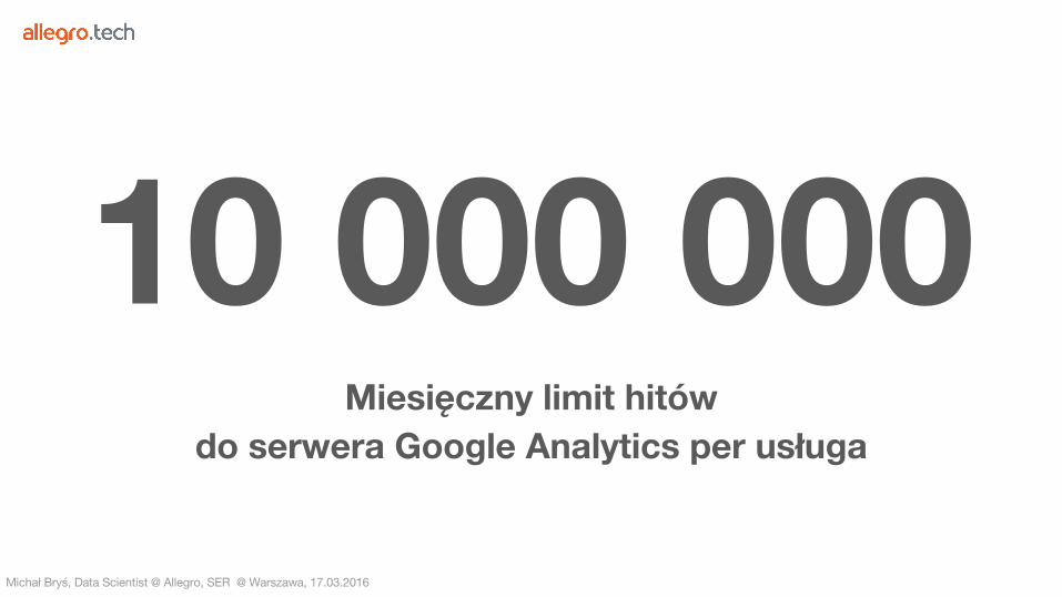
20 praktyczny aspektów Google Analytics - In Digital Marketing 6.10.2016
Upload
michal-brysCategory
view
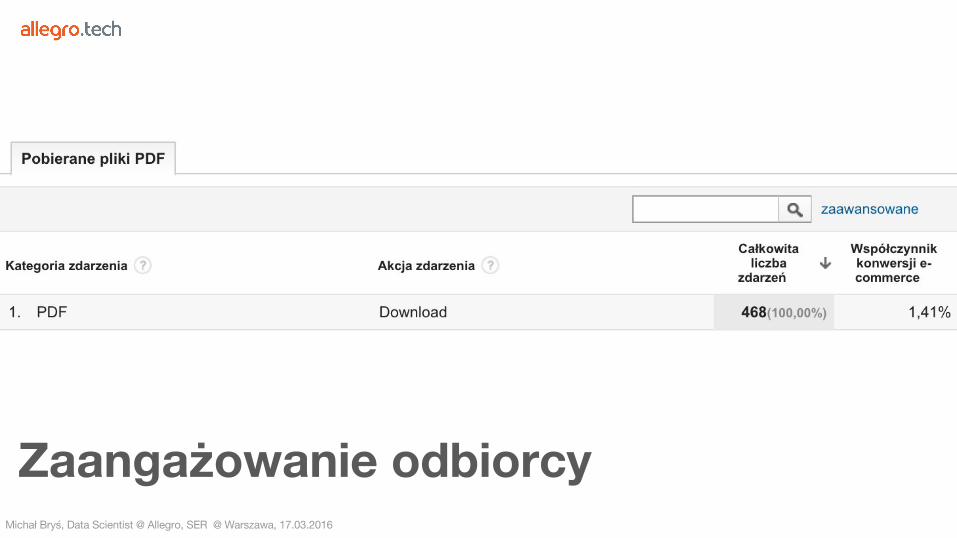
751download
0


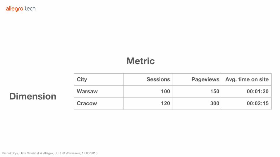
100 150 00:01:20
120 300 00:02:15

●●●●●●

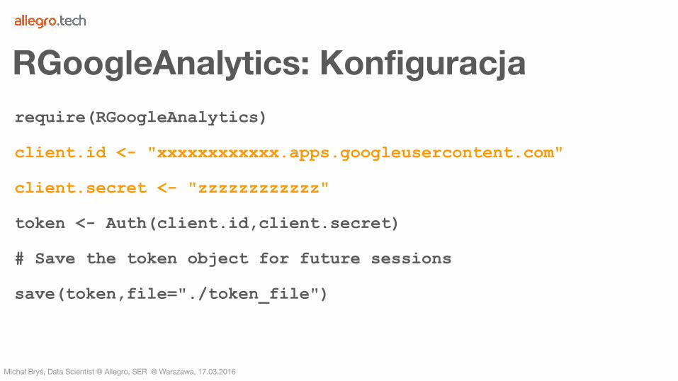
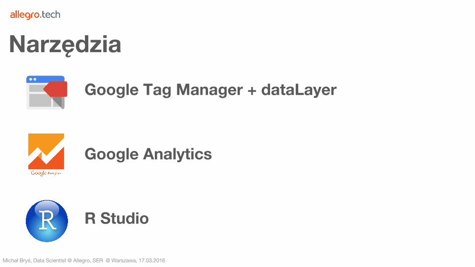
require(RGoogleAnalytics)
client.id <- "xxxxxxxxxxxx.apps.googleusercontent.com"
client.secret <- "zzzzzzzzzzzz"
token <- Auth(client.id,client.secret)
# Save the token object for future sessions
save(token,file="./token_file")
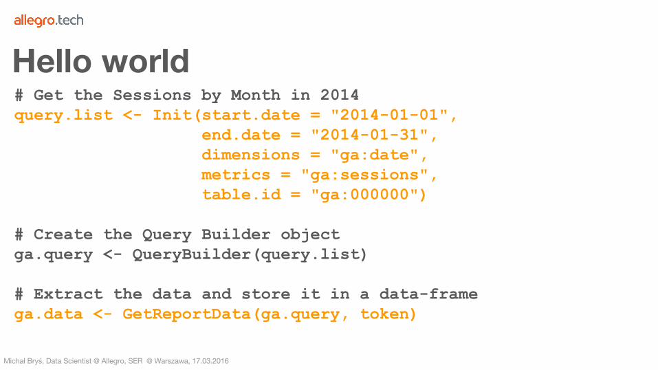
# Get the Sessions by Month in 2014query.list <- Init(start.date = "2014-01-01", end.date = "2014-01-31", dimensions = "ga:date", metrics = "ga:sessions", table.id = "ga:000000")
# Create the Query Builder objectga.query <- QueryBuilder(query.list)
# Extract the data and store it in a data-framega.data <- GetReportData(ga.query, token)

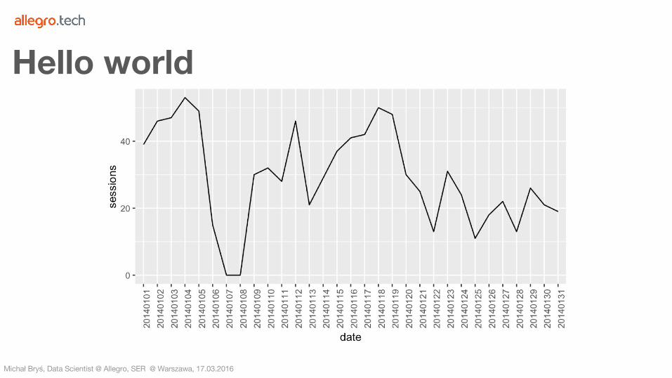
> head(ga.data)
date sessions1 20140101 392 20140102 463 20140103 474 20140104 535 20140105 496 20140106 15
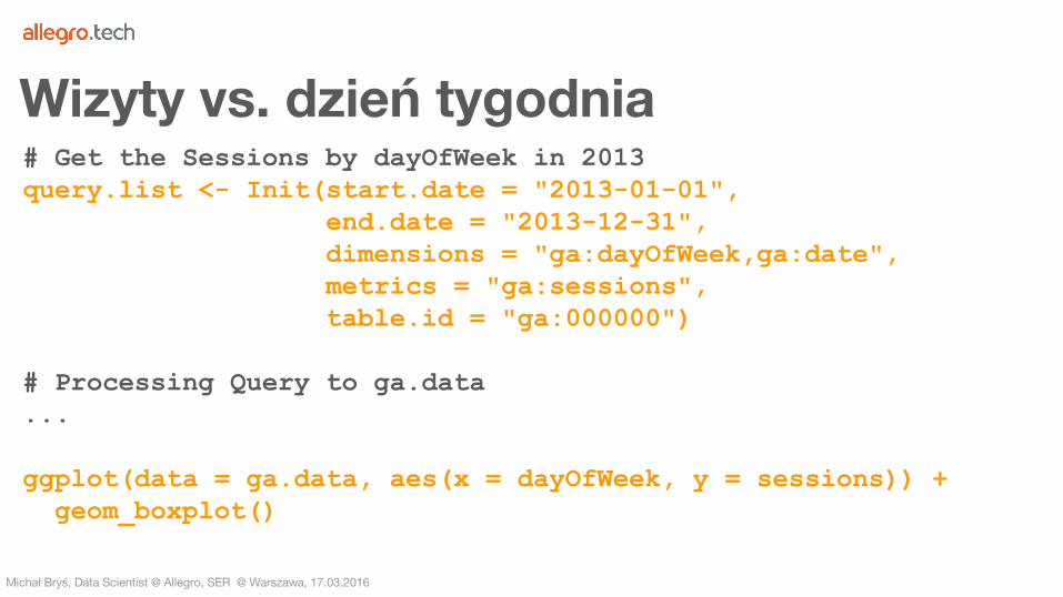
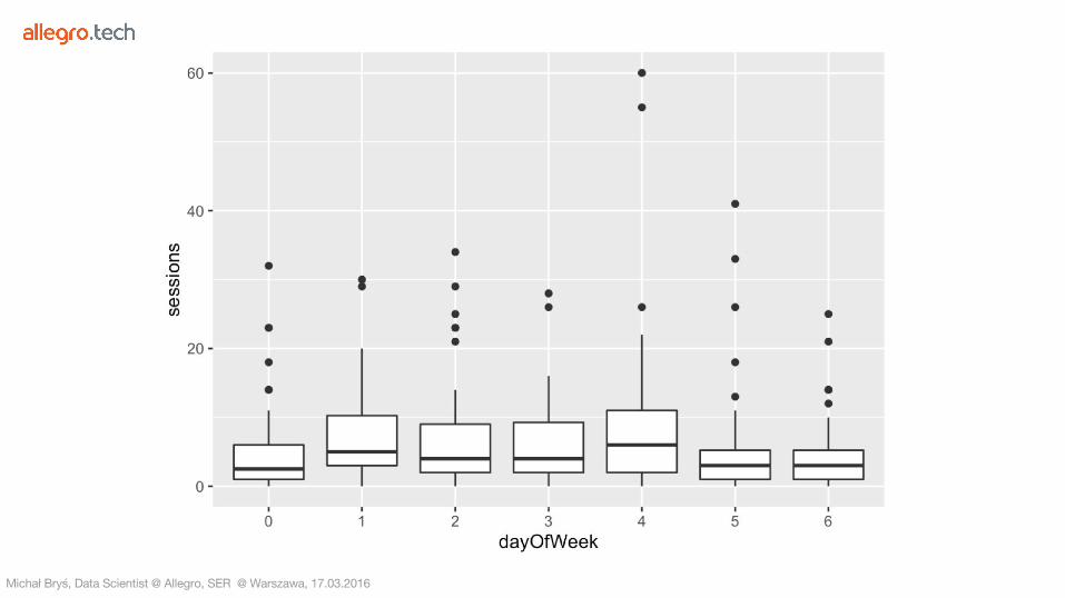
# Get the Sessions by dayOfWeek in 2013query.list <- Init(start.date = "2013-01-01", end.date = "2013-12-31", dimensions = "ga:dayOfWeek,ga:date", metrics = "ga:sessions", table.id = "ga:000000")
# Processing Query to ga.data...
ggplot(data = ga.data, aes(x = dayOfWeek, y = sessions)) + geom_boxplot()
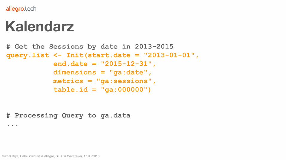
# Get the Sessions by date in 2013-2015query.list <- Init(start.date = "2013-01-01", end.date = "2015-12-31", dimensions = "ga:date", metrics = "ga:sessions", table.id = "ga:000000")
# Processing Query to ga.data...
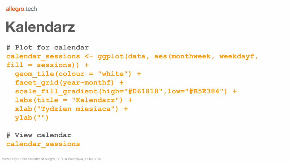
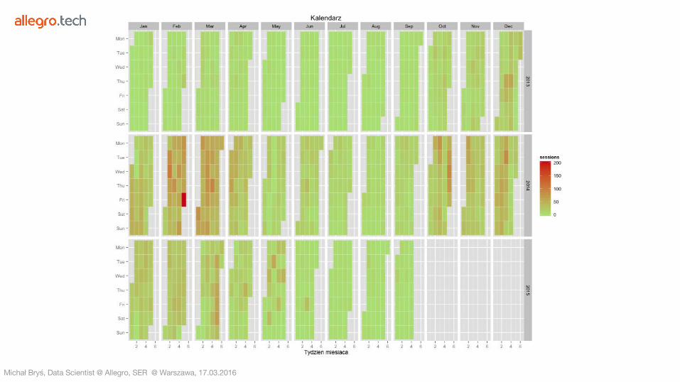
# Plot for calendarcalendar_sessions <- ggplot(data, aes(monthweek, weekdayf, fill = sessions)) + geom_tile(colour = "white") + facet_grid(year~monthf) + scale_fill_gradient(high="#D61818",low="#B5E384") + labs(title = "Kalendarz") + xlab("Tydzien miesiaca") + ylab("")
# View calendarcalendar_sessions
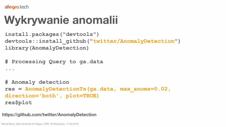
install.packages("devtools")devtools::install_github("twitter/AnomalyDetection")library(AnomalyDetection)
# Processing Query to ga.data...
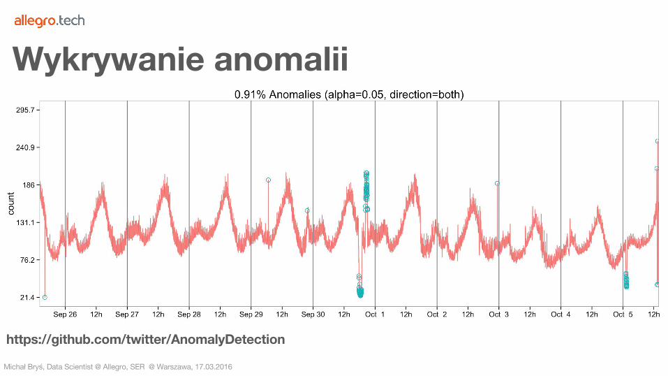
# Anomaly detectionres = AnomalyDetectionTs(ga.data, max_anoms=0.02, direction='both', plot=TRUE)res$plot
...
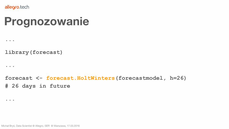
library(forecast)
...
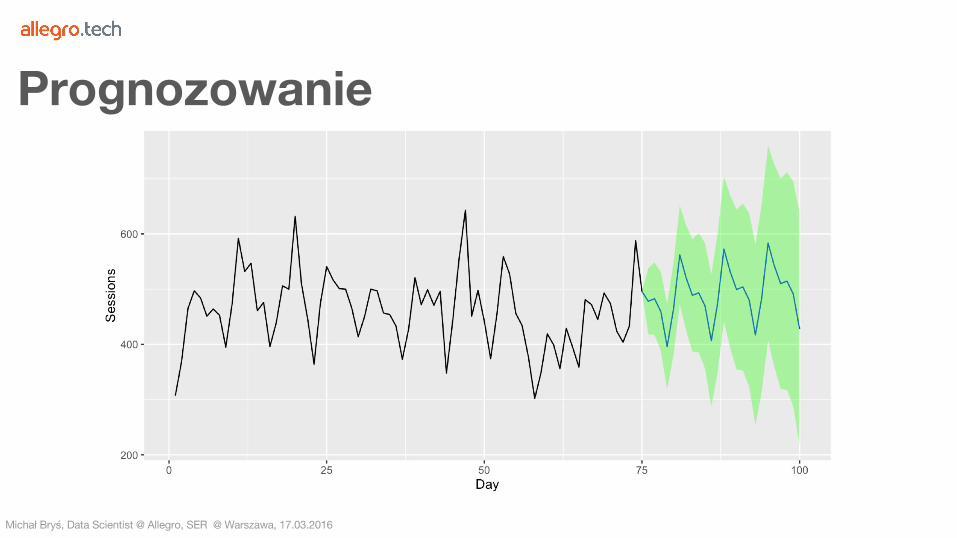
forecast <- forecast.HoltWinters(forecastmodel, h=26) # 26 days in future
...


●●

●○
●○

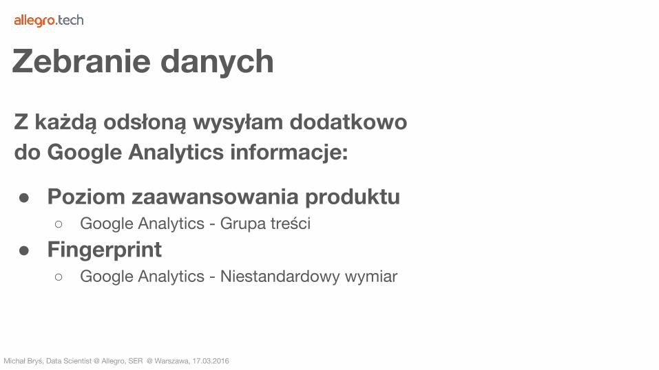
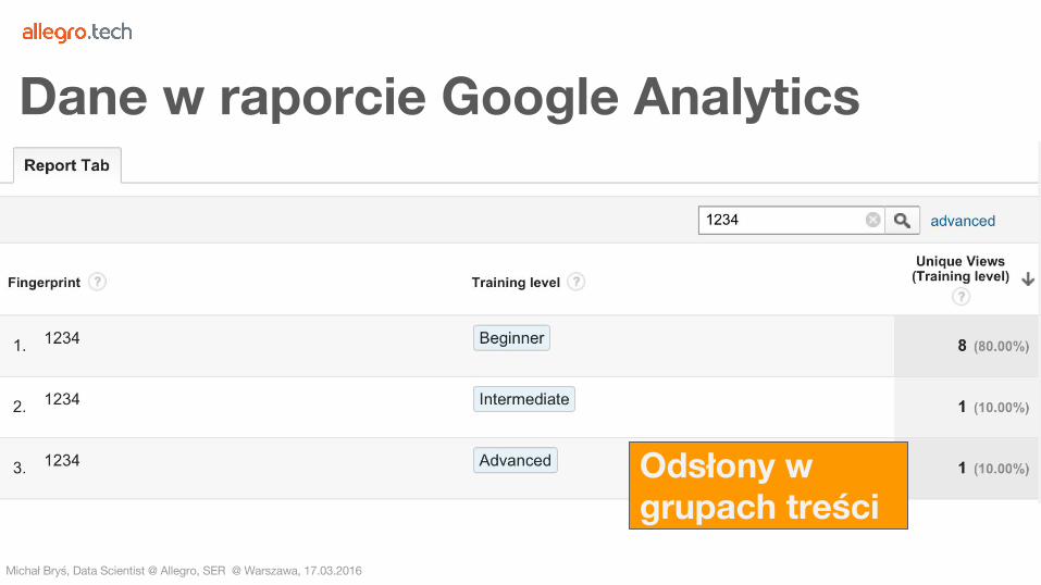
<script> dataLayer = [{ 'level': 'advanced',
'fingerprint' : '123456' }];</script>
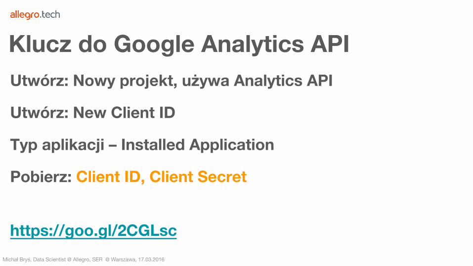
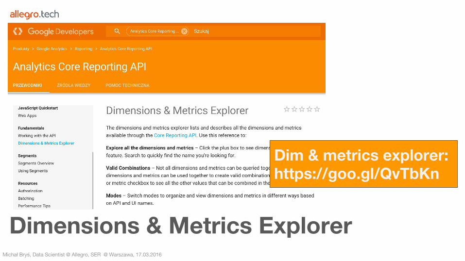
https://goo.gl/1X84fY
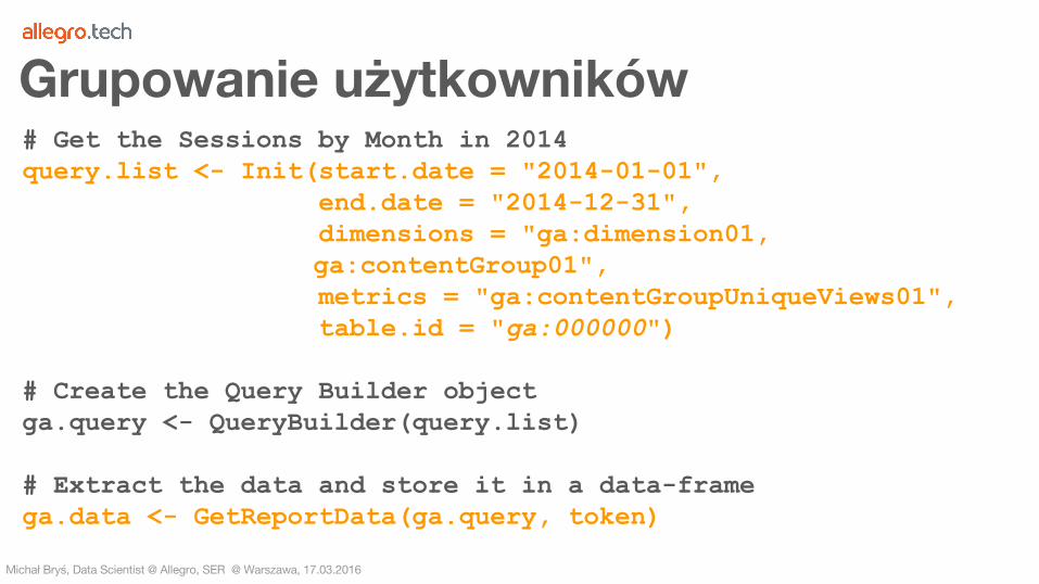
# Get the Sessions by Month in 2014query.list <- Init(start.date = "2014-01-01", end.date = "2014-12-31", dimensions = "ga:dimension01,
ga:contentGroup01", metrics = "ga:contentGroupUniqueViews01", table.id = "ga:000000")
# Create the Query Builder objectga.query <- QueryBuilder(query.list)
# Extract the data and store it in a data-framega.data <- GetReportData(ga.query, token)
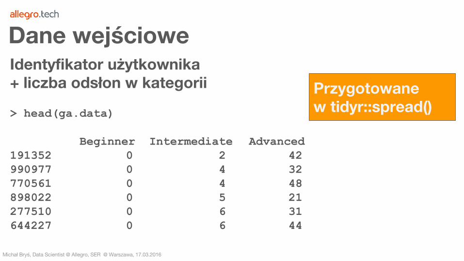
> head(ga.data)
Beginner Intermediate Advanced191352 0 2 42990977 0 4 32770561 0 4 48898022 0 5 21277510 0 6 31644227 0 6 44
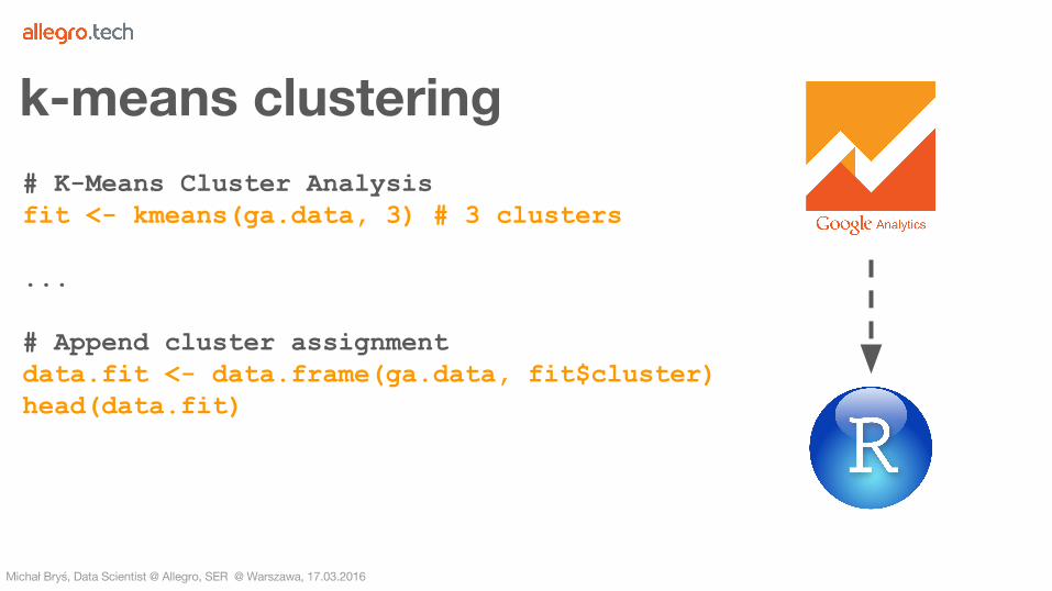
# K-Means Cluster Analysisfit <- kmeans(ga.data, 3) # 3 clusters
...
# Append cluster assignmentdata.fit <- data.frame(ga.data, fit$cluster)head(data.fit)
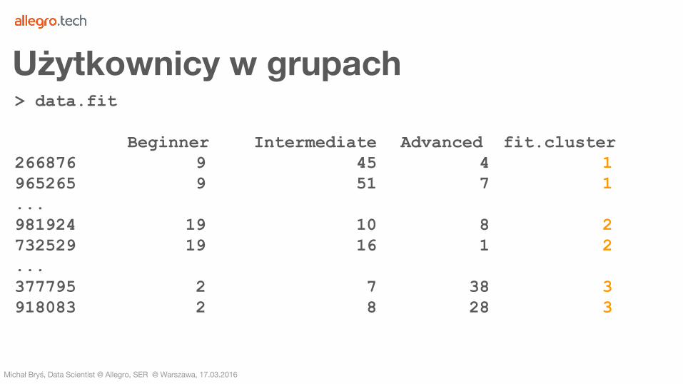
> data.fit
Beginner Intermediate Advanced fit.cluster266876 9 45 4 1965265 9 51 7 1...981924 19 10 8 2732529 19 16 1 2...377795 2 7 38 3918083 2 8 28 3
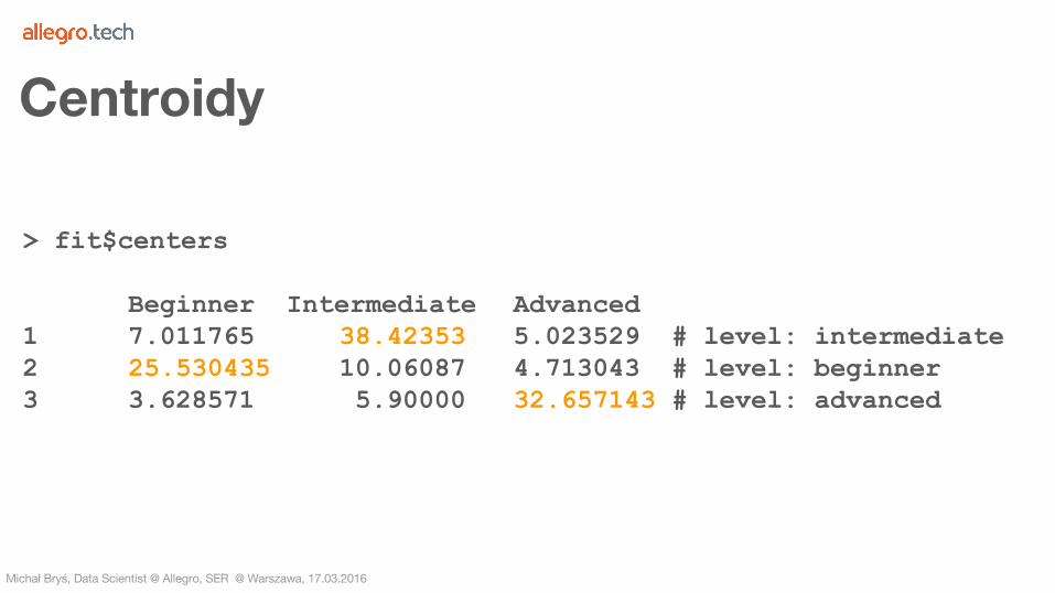
> fit$centers
Beginner Intermediate Advanced1 7.011765 38.42353 5.023529 # level: intermediate2 25.530435 10.06087 4.713043 # level: beginner3 3.628571 5.90000 32.657143 # level: advanced
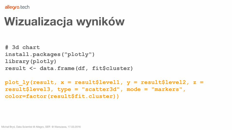
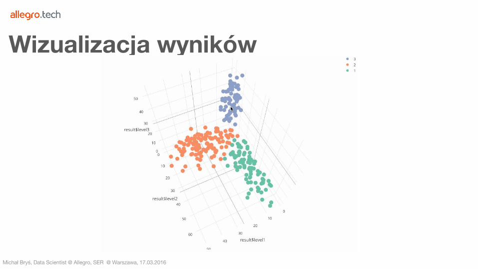
# 3d chartinstall.packages("plotly")library(plotly)result <- data.frame(df, fit$cluster)
plot_ly(result, x = result$level1, y = result$level2, z = result$level3, type = "scatter3d", mode = "markers", color=factor(result$fit.cluster))