
MODELING AND OPTIMIZATION OF COMPUTER … Informatics and Control... · the field of computer...
148
Projekt współfinansowany ze środków Unii Europejskiej w ramach Europejskiego Funduszu Społecznego ROZWÓJ POTENCJAŁU I OFERTY DYDAKTYCZNEJ POLITECHNIKI WROCŁAWSKIEJ Wrocław University of Technology Advanced Informatics and Control Krzysztof Walkowiak MODELING AND OPTIMIZATION OF COMPUTER NETWORKS Developing Engine Technology Wrocław 2011
-
Upload
hoangxuyen -
Category
Documents
-
view
216 -
download
1
Transcript of MODELING AND OPTIMIZATION OF COMPUTER … Informatics and Control... · the field of computer...
Projekt współfinansowany ze środków Unii Europejskiej w ramach Europejskiego Funduszu Społecznego
ROZWÓJ POTENCJAŁU I OFERTY DYDAKTYCZNEJ POLITECHNIKI WROCŁAWSKIEJ
Wrocław University of Technology
Advanced Informatics and Control
Krzysztof Walkowiak
MODELING AND OPTIMIZATION
OF COMPUTER NETWORKS Developing Engine Technology
Wrocław 2011

Wrocław University of Technology
Advanced Informatics and Control
Krzysztof Walkowiak
MODELING AND OPTIMIZATION OF COMPUTER NETWORKS
Developing Engine Technology
Wrocław 2011

Copyright © by Wrocław University of Technology
Wrocław 2011
Reviewer: Andrzej Kasprzak
ISBN 978-83-62098-34-7
Published by PRINTPAP Łódź, www.printpap.pl

1. Introduction ................................................................................................................... 5
2. Technology Related Examples ..................................................................................... 8
2.1. Tunnels Optimization in MPLS Networks ............................................................ 8
2.2. Routing and Wavelength Assignment in Optical Networks ................................ 10
2.3. MPLS over GE Network Design ......................................................................... 13
2.4. SONET/SDH Protection ...................................................................................... 15
2.5. Dimensioning of Overlay Networks for P2P Multicasting .................................. 17
2.6. Access Point Location in WLANs ....................................................................... 19
2.7. Exercises .............................................................................................................. 21
3. Multicommodity Flows ............................................................................................... 22
3.1. One Commodity Flow ......................................................................................... 22
3.2. Multicommodity Flows ........................................................................................ 23
3.3. Types of Multicommodity Flows ........................................................................ 26
4. Flow Optimization ...................................................................................................... 28
4.1. Bifurcated Flows with Linear Objective Function .............................................. 28
4.2. Bifurcated Flows with Convex Objective Function ............................................ 32
4.3. Non-bifurcated Flows .......................................................................................... 35
4.4. Non-bifurcated Congestion Problem ................................................................... 41
4.5. Example ............................................................................................................... 44
4.6. Exercises .............................................................................................................. 49
5. Capacity and Flow Optimization ................................................................................ 51
5.1. Bifurcated Flows with Linear Objective Function .............................................. 51
5.2. Routing Restrictions ............................................................................................ 55
5.3. Link Modularity ................................................................................................... 57
5.4. Convex Problems ................................................................................................. 60
5.5. Example ............................................................................................................... 62
5.6. Exercises .............................................................................................................. 65
6. Multicast Flows ........................................................................................................... 66
6.1. Modeling of Multicast Flows ............................................................................... 67
6.2. Cost Problem ........................................................................................................ 74
6.3. Network Design Problem ..................................................................................... 75
6.4. Maximum Delay Problem .................................................................................... 77
6.5. Throughput Problem ............................................................................................ 78
6.6. Multicast Packing Problem .................................................................................. 80
3
6.7. Root Location Problem ........................................................................................ 81
6.8. Exercises .............................................................................................................. 83
7. Anycast Flows ............................................................................................................. 84
7.1. Modeling of Anycast Flows ................................................................................. 86
7.2. Flow Allocation Problem ..................................................................................... 92
7.3. Network Design Problem ..................................................................................... 95
7.4. Lost Flow Problem ............................................................................................... 96
7.5. Replica Location Problem ................................................................................... 99
7.6. Multi-Layer Networks ....................................................................................... 101
7.7. Exercises ............................................................................................................ 105
8. Peer-to-Peer Flows .................................................................................................... 106
8.1. Modeling of P2P Flows ..................................................................................... 107
8.2. Synchronous P2P Cost Problem ........................................................................ 112
8.3. Other Formulations of Synchronous P2P Problems .......................................... 115
8.4. P2P Multicast Network Design Problem ........................................................... 116
8.5. Survivable P2P Multicasting ............................................................................. 121
8.6. Exercises ............................................................................................................ 125
9. Distributed Computing Systems ............................................................................... 126
9.1. Overlay Cost Problem ........................................................................................ 127
9.2. Network Cost Problem ....................................................................................... 130
9.3. Response Time Problem .................................................................................... 132
9.4. Synchronous P2P System .................................................................................. 136
9.5. Exercises ............................................................................................................ 140
Bibliography ................................................................................................................. 142
4
1. Introduction
The research community from both academia and industry started studying various
issues related to modeling and optimization of communication networks at the same
time when the progress of communication networks was noticeable. The main
motivation behind this fact was to provide efficient optimization tools to enable
development of various kinds of communication networks satisfying clients’ needs in a
cost effective manner. At the beginning, the research was quite narrow and limited to
telephone networks. However, the advent of the Internet and next other kinds of
communication networks (e.g., mobile networks) as well as the process of network
convergence triggered much faster and wider research in the field of modeling and
optimization of computer networks. Consequently, nowadays we can witness numerous
scientific journals and conferences devoted to this topic. Moreover, large vendors of
network equipment and telecoms develop R&D centers to make research on these
issues. The prognosis for the future is that – due to very fast development of new
technologies, protocols, services and growing popularity of computer networks all over
the world – emerging problems related to modeling and optimization of computer
networks will focus the attention of researchers for a long time.
The main purpose of this book is to present basic information related to
modeling and optimization of computer networks. We present models and algorithms
for optimization of various elements of computer networks including routing, link
capacity and resource location. An important novelty of this textbook – comparing to
earlier books – is that we consider various kinds of network flows. Most of previous
research in the field of modeling and optimization of computer networks is restricted to
unicast flows. We extend this scope to other kinds of network flows including anycast,
multicast and Peer-to-Peer. Moreover, we present information related to optimization of
network oriented distributed computing systems. The idea behind the extended range of
the book is to present classical models and methods related to the research conducted in
the field of computer network optimization for many years as well as to show latest
topics that have been attracting considerable attention from researchers recently.
It is assumed that the reader of this book has some basic knowledge regarding
computer networks, technologies and protocols as well optimization methods and
algorithms. However, if some parts and information presented in the remainder of this
book are not understandable, the reader is referred to books and other works presenting:
5
• basic issues of computer networks (e.g., [PER05], [Tan03], [RVC01]);
• various concepts of distributed computing systems including Peer-to-Peer
networks, content delivery, multicasting, distributed computing, (e.g., [BYL09],
[HB05], [Min08], [NSW04], [SYB09], [Pen04], [SW05], [Tar10]);
• issues of network survivability, (e.g., [Gro04], [PM04], [VPD04]);
• optimization methods and modeling (e.g., [Gro04], [Kas01], [Kle64], [KT05],
[PM04], [Tal09], [Wal08a]).
The remaining part of the book is divided into nine sections. Chapter 2 presents
several technology related examples showing how to model problems following from
real network technologies. In Chapter 3, we introduce the multicommodity flow
modeling, which is the main tool used in research on optimization of various kinds of
computer networks. Chapter 4 focuses on optimization of flows in existing networks –
we consider various kinds of flows (bifurcated and non-bifurcated) and different
objective functions (linear and convex). In Chapter 5, we address a broad range of
network design problems related to joint optimization of link capacity and network
flows. Starting from Chapter 6, we concentrate on very recent issues related to
optimization of various distributed systems and network survivability. Chapter 6
presents models of multicast flows currently applied inter alia to streaming services like
IPTV, Internet radio, Video on Demand. In Chapter 7, we concentrate on anycast flows
that are used in various replication and caching systems including Content Delivery
Networks (CDNs). Chapter 8 addresses the problems of modeling and optimization of
Peer-to-Peer flows – popular network concept broadly used in many latest network
services. In Chapter 9, we focus on distributed computing systems developed to answer
the growing need for computational power in both academia and industry.
There are two important topics related to the current research on modeling and
optimization of computer networks that this book presents only in a brief way: network
survivability and multi-layer networks. Issues related to network survivability have been
gaining large attention corresponding to the growing role of computer networks and the
fact that a network failure could cause a lot of damages including economic loses,
political conflicts, human health problems. We mention this problem in Section 8.5 in
the context of P2P multicasting. For further information on the research related to
modeling and optimization of survivable networks see [Gro04], [PM04], [Wal07a],
[Wal08a], [Wal09b], [VPD04]. The majority of optimization models presented in this
6
book assume that the network consists of a single layer. While most existing networks
uses many various technologies and protocols and the real network structured must be
modeled as a set of different layers (e.g., MPLS over DWDM) with specific constraints
connecting the adjacent layers. The issues of multi-layer networks are presented in the
context of anycast flows in Chapter 7. For a good survey on multilayer networks refer to
[PM04] and other works on this topic in recent proceedings and journals.
7
2. Technology Related Examples
In this chapter we present several modeling examples related to existing network
technologies. The motivation is to show the whole process of the model construction
starting from analysis of the technology in order to write the problem as an optimization
model with variables, constants, objective function and constraints. To model network
traffic various versions of multicommodity flows are used. For more details of
multicommodity flows refer to Chapter 3. Note that the modeling is usually a tradeoff
between size/complexity of the model and the level of technological details.
2.1. Tunnels Optimization in MPLS Networks
First, we present model of tunnels optimization in MPLS networks [PM04]. The
MultiProtocol Label Switching (MPLS) approach proposed by the Internet Engineering
Task Force (IETF) [RVC01] is a networking technology that enables delivering of
traffic engineering capability and QoS performance for carrier networks. The MPLS
network consists of two types of devices:
• Label Edge Router (LER) located on the entry and exit points of the MPLS
network.
• Label Switch Routers (LSR) located inside the MPLS network.
In the MPLS network packets are sent along LSP (Label Switch Path) between
LERs and LSRs. The LER pushes an MPLS label onto an incoming packet and pop it
off the outgoing packet according to the FEC (Forwarding Equivalence Class). To
classify a packet to a FEC class an IP address or other element of the header (e.g.,
DSCP) can be applied. Different FEC classes can have various QoS parameters, thus we
can send in the network a variety types of traffic. Consequently, packets (included in
different FEC classes) between the same pair of nodes can use different paths (routes).
This enables effective traffic engineering. For more information on MPLS refer to
[Gro04], [PER05], [PM04], [RVC01], [VPD04].
The objective of the considered optimization problem is to carry different traffic
classes in an MPLS network through the creation of tunnels in such a way that the
number of tunnels on each MPLS router/link is minimized and load balanced. We are
given with the network topology, link capacity, demands and candidate paths.
Now we introduce a mathematical model of the problem. We use the notation as
in [PM04]. Let identifier d = 1,2,…,D denote a demand defined by source and
8

destination nodes and volume (bandwidth) hd. The volume hd of demand d can be
carried over multiple tunnels (paths) from ingress to egress MPLS LERs. We use index
p = 1,2,…,Pd to denote candidate paths for demand d. Each candidate path of demand d
starts at the source node of demand d and terminates in the destination node of d.
Constant δedp denotes the path p of demand d and is 1, if link e belongs to path p
realizing demand d and 0 otherwise.
The fraction of the demand volume for demand d to be carried on tunnel p is
denoted as xdp. Note that xdp is a continuous decision variable. Since the whole demand
volume is to be transmitted in the network for each demand, we have the demand
constraint, which guarantees that the sum of all fractional flows xdp over all candidate
paths p = 1,2,…,Pd must add up to the whole demand volume hd
∑p xdp = 1, d = 1,2,…,D. (2.1.1)
Since a flow can have very small fraction, we propose to set a lower bound on
the fraction of a flow on a path. We use a positive quantity ε to be the lower bound on
fraction of flow on a tunnel (path). We use the binary variable udp = 1 to denote
selection of a tunnel, if the lower bound is satisfied (and 0, otherwise). We introduce the
following two constraints:
εudp ≤ xdphd, d = 1,2,…,D p = 1,2,…,Pd (2.1.2)
xdp ≤ udp, d = 1,2,…,D p = 1,2,…,Pd. (2.1.3)
Condition (2.1.2) assures that if a tunnel is selected, then the tunnel must have at
least the fraction of allocated flow which is set to ε. Constraint (2.1.3) guarantees that if
a tunnel is not selected, then the flow fraction associated with this tunnel should be
forced to be equal to 0. Since the network is given and link capacity is known, we must
assure the physical link capacity ce of link e is not exceeded. Thus, we formulate the
capacity constraint:
∑d hd∑p δedpxdp ≤ ce, e = 1,2,…,E. (2.1.4)
Notice that the left-hand side of (2.1.4) is the flow on link e calculated taking
into account all demands d = 1,2,…,D and candidate paths p = 1,2,…,Pd and checking if
the given demand d uses path p (δedp = 1) and considering the flow fraction xdp. The
number of tunnels on link e is given by formula ∑d∑p δedpudp. Let r denote the maximum
number of tunnels on a link. Therefore, we write the following constraint:
∑d∑p δedpudp ≤ r, e = 1,2,…,E. (2.1.5)
9
Since the goal of optimization is to minimize the total number of tunnels, the
objective minimizes a number r that represents the maximum number of tunnels over all
links. The whole model can be written in the following way.
Tunnels Optimization in MPLS �etworks Model
indices
d = 1,2,…,D demands
p = 1,2,…,Pd candidate paths for demand d
e = 1,2,…,E network links
constants
δedp = 1, if link e belongs to path p realizing demand d; 0, otherwise
hd volume of unicast demand d
ce capacity of link e
ε lower bound on fraction of flow on a tunnel (path)
variables
xdp fractional flow allocated to path p of demand d (continuous non-
negative)
udp =1, if path p is selected to carry part of demand d; 0, otherwise
r maximum number of tunnels on a link
objective
minimize F = r
subject to
∑p xdp = 1, d = 1,2,…,D
∑d hd∑p δedpxdp ≤ ce, e = 1,2,…,E
εudp ≤ xdphd, d = 1,2,…,D p = 1,2,…,Pd
xdp ≤ udp, d = 1,2,…,D p = 1,2,…,Pd
∑d∑p δedpudp ≤ r, e = 1,2,…,E.
For more details on tunnels optimization in MPLS networks see [PM04].
2.2. Routing and Wavelength Assignment in Optical Networks
WDM (Wavelength Division Multiplexing) is an optical technology, which multiplexes
multiple optical signals on a single optical fiber by using different wavelengths (colors)
10
of laser light to carry different signals. Note that the WDM is a connection-oriented
technique, since the whole signal is transmitted along one path. Optical devices mostly
cannot covert the wavelength, therefore the whole connection must use the same color
(no wavelength conversion). For more information on optical networks refer to [Gro04],
[PER05], [VPD04].
In the Routing and Wavelength Assignment (RWA) problem the capacity of
each link is given [JMT06]. It has been proven to be a NP-complete problem. Two
possible objective functions can be used in the RWA:
• Given maximal capacity, i.e., maximize routed traffic (throughput).
• Offered traffic given, i.e., minimize wavelength requirement.
We consider the latter function, i.e., the objective of our problem is to minimize
the number of wavelengths. We are given: network topology, link capacity, demands
(lightpaths). Moreover, we assume that the wavelength conversion is not possible in the
network.
Let d = 1,2,…,D denote a demand defined as a node pair sd and td. Demand d
requires hd connections (lightpaths) to be routed in the network. Let aev is 1, if link e
originates at node v and 0, otherwise. Analogously, let bev = 1, if link e terminates in
node v; 0, otherwise. Λ denotes the number of wavelengths per fiber and λ is a
wavelength index (λ = 1,2,…,Λ). Since we consider the WDM network, single path
routing is applied (non-bifurcated multicommodity flows). Binary variable xdλ is 1, if
demand d uses wavelength λ; 0, otherwise. Another binary variable xedλ is 1, if demand
d uses wavelength λ on link e; 0, otherwise. The model uses classical multicommodity
flow formulation, however an additional layer of each wavelength λ is considered.
Therefore, we formulate the following flow conservation constraints:
∑e aevxedλ – ∑e bevxedλ = xdλ, if v = sd v = 1,2,…,V d = 1,2,…,D
λ = 1,2,…,Λ (2.2.1)
∑e aevxedλ – ∑e bevxedλ = –xdλ, if v = td v = 1,2,…,V d = 1,2,…,D
λ = 1,2,…,Λ (2.2.2)
∑e aevxedλ – ∑e bevxedλ = 0, if v ≠ sd,td v = 1,2,…,V d = 1,2,…,D
λ = 1,2,…,Λ. (2.2.3)
Notice that the left-hand side of above constraints is the number of links used by
demand d and allocated to wavelength λ leaving node v minus the number of links used
by demand d and allocated to wavelength λ entering node v. If the node v is the source
11

node of demand d (v = sd), the right-hand side is equal to xdλ, i.e., if wavelength λ is used
by demand d, the value is 1 (constraint (2.2.1)). Similarly, if the node v is the
destination node of demand d (v = td), the right-hand side is equal to –xdλ, i.e., if
wavelength λ is used by demand d, the value is –1 (constraint (2.2.2)). Finally, for all
remaining (transit) nodes (v ≠ sd,td), the right-hand side is 0 (constraint (2.2.3)).
The next constraint states that the whole demand hd must be satisfied, i.e., there
must be provided hd lightpaths for each demand:
∑λ xdλ = hd, d = 1,2,…,D. (2.2.4)
We introduce another binary variable xλ which denotes if wavelength λ is used in
the network. Variable xλ is defined by the following constraint:
xdλ ≤ xλ, d = 1,2,…,D λ = 1,2,…,Λ. (2.2.5)
The following clash constraint expresses that no two lightpaths going through
the same fiber link can use the same wavelength:
∑d xedλ ≤ xλ, e = 1,2,…,E λ = 1,2,…,Λ. (2.2.6)
The number of wavelengths used in the network is given by ∑λ xλ. Note that in
the model we do not include the capacity constraint as in the previous example (2.1.4).
This follows from the fact that we are given a set of possible wavelengths, and in this
way we set an upper limit on the link capacity. The whole model is formulated as
follows.
Routing and Wavelength Assignment Problem
indices
v = 1,2,…,V network nodes
d = 1,2,…,D demands
e = 1,2,…,E network links
λ = 1,2,…,Λ lambdas (wavelengths)
constants
aev = 1, if link e originates at node v; 0, otherwise
bev = 1, if link e terminates in node v; 0, otherwise
sd source node of demand d
td destination node of demand d
hd volume of unicast demand d
variables
12
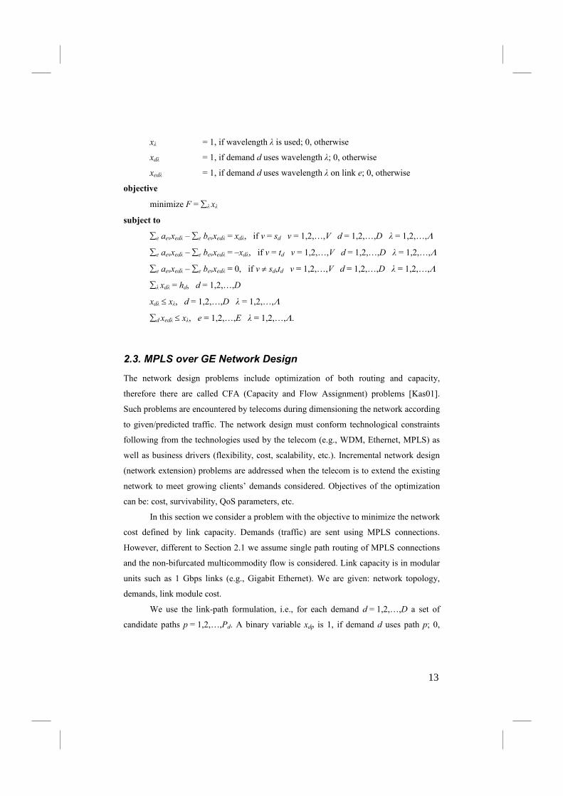
xλ = 1, if wavelength λ is used; 0, otherwise
xdλ = 1, if demand d uses wavelength λ; 0, otherwise
xedλ = 1, if demand d uses wavelength λ on link e; 0, otherwise
objective
minimize F = ∑λ xλ
subject to
∑e aevxedλ – ∑e bevxedλ = xdλ, if v = sd v = 1,2,…,V d = 1,2,…,D λ = 1,2,…,Λ
∑e aevxedλ – ∑e bevxedλ = –xdλ, if v = td v = 1,2,…,V d = 1,2,…,D λ = 1,2,…,Λ
∑e aevxedλ – ∑e bevxedλ = 0, if v ≠ sd,td v = 1,2,…,V d = 1,2,…,D λ = 1,2,…,Λ
∑λ xdλ = hd, d = 1,2,…,D
xdλ ≤ xλ, d = 1,2,…,D λ = 1,2,…,Λ
∑d xedλ ≤ xλ, e = 1,2,…,E λ = 1,2,…,Λ.
2.3. MPLS over GE Network Design
The network design problems include optimization of both routing and capacity,
therefore there are called CFA (Capacity and Flow Assignment) problems [Kas01].
Such problems are encountered by telecoms during dimensioning the network according
to given/predicted traffic. The network design must conform technological constraints
following from the technologies used by the telecom (e.g., WDM, Ethernet, MPLS) as
well as business drivers (flexibility, cost, scalability, etc.). Incremental network design
(network extension) problems are addressed when the telecom is to extend the existing
network to meet growing clients’ demands considered. Objectives of the optimization
can be: cost, survivability, QoS parameters, etc.
In this section we consider a problem with the objective to minimize the network
cost defined by link capacity. Demands (traffic) are sent using MPLS connections.
However, different to Section 2.1 we assume single path routing of MPLS connections
and the non-bifurcated multicommodity flow is considered. Link capacity is in modular
units such as 1 Gbps links (e.g., Gigabit Ethernet). We are given: network topology,
demands, link module cost.
We use the link-path formulation, i.e., for each demand d = 1,2,…,D a set of
candidate paths p = 1,2,…,Pd. A binary variable xdp is 1, if demand d uses path p; 0,
13

otherwise. Since the non-bifurcated flow is used and only one path can be selected for
demand d, we formulate the demand constraint as follows:
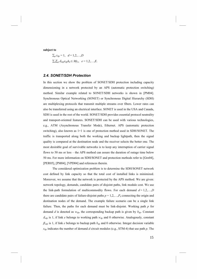
∑p xdp = 1, d = 1,2,…,D. (2.3.1)
Constant δedp denotes that path p of demand d and is 1, if link e belongs to path p
realizing demand d; 0, otherwise. The demand volume is given by hd (bps). The flow on
each link e is given by formula ∑d∑p δedpxdphd, which is similar to (2.1.4). However,
since the decision variable is binary, we also introduce to the formula the demand
volume hd.
Integer variable ye denotes the number of capacity modules installed on link e, M
is the size of one module (e.g., 1 Gbps). Moreover, we assume that ξe is a cost of one
module in link e (e.g., given in Euro). Consequently, the total network cost is given by
∑e yeξe. The capacity constraint saying that the flow on each link e cannot exceed the
link capacity is formulated in the following way:
∑d∑p δedpxdphd ≤ yeM, e = 1,2,…,E. (2.3.2)
MPLS over GE �etwork Design Problem
indices
d = 1,2,…,D demands
p = 1,2,…,Pd candidate paths for demand d
e = 1,2,…,E network links
constants
δedp = 1, if link e belongs to path p realizing demand d; 0, otherwise
hd volume of unicast demand d
ξe unit (marginal) cost of link e
M size of one capacity module (e.g., 1 Gbps)
variables
xdp = 1, if path p is used to realize demand d; 0, otherwise (binary)
ye capacity of link e as the number of modules (non-negative
integer)
objective
minimize F = ∑e ξeye
14
subject to
∑p xdp = 1, d = 1,2,…,D
∑d∑p δedpxdphd ≤ Mye, e = 1,2,…,E.
2.4. SONET/SDH Protection
In this section we show the problem of SONET/SDH protection including capacity
dimensioning in a network protected by an APS (automatic protection switching)
method. Similar example related to SONET/SDH networks is shown in [PM04].
Synchronous Optical Networking (SONET) or Synchronous Digital Hierarchy (SDH)
are multiplexing protocols that transmit multiple streams over fibers. Lower rates can
also be transferred using an electrical interface. SONET is used in the USA and Canada,
SDH is used in the rest of the world. SONET/SDH provides essential protocol neutrality
and transport-oriented features. SONET/SDH can be used with various technologies,
e.g., ATM (Asynchronous Transfer Mode), Ethernet. APS (automatic protection
switching), also known as 1+1 is one of protection method used in SDH/SONET. The
traffic is transported along both the working and backup lightpath, then the signal
quality is compared at the destination node and the receiver selects the better one. The
most desirable goal of survivable networks is to keep any interruption of carrier signal
flows to 50 ms or less – the APS method can assure the duration of outage time below
50 ms. For more information on SDH/SONET and protection methods refer to [Gro04],
[PER05], [PM04], [VPD04] and references therein.
The considered optimization problem is to determine the SDH/SONET network
cost defined by link capacity so that the total cost of installed links is minimized.
Moreover, we assume that the network is protected by the APS method. We are given:
network topology, demands, candidate pairs of disjoint paths, link module cost. We use
the link-path formulation of multicommodity flows. For each demand d = 1,2,…,D
there are candidate pairs of failure-disjoint paths p = 1,2,…,Pd connecting the origin and
destination nodes of the demand. The example failure scenario can be a single link
failure. Then, the paths for each demand must be link-disjoint. Working path p for
demand d is denoted as wdp, the corresponding backup path is given by bdp. Constant
δedp is 1, if link e belongs to working path wdp and 0 otherwise. Analogously, constant
βedp is 1, if link e belongs to backup path bdp and 0 otherwise. Integer decision variable
xdp indicates the number of demand d circuit modules (e.g., STM-4) that use path p. The
15

volume of demand d is given by hd (given in circuit modules). Therefore, the demand
constraint is as follows:
∑p xdp = hd, d = 1,2,…,D. (2.4.1)
The flow on link e related to working paths is ∑d∑p xdpδedp. The corresponding
flow on link e related to backup paths is ∑d∑p xdpβedp, i.e., the backup paths have a
reserved capacity of the case of a network failure. The variable ye denotes the number of
capacity modules installed on link e. Constant M denotes the size of one module (e.g.,
STM-4) and ξe is cost of one module in link e. Thus, the network cost is given by
∑e yeξe. Capacity constraint stating that flow on each link cannot exceed the link
capacity is formulated in the following way:
∑d∑p xdp(δedp + βedp) ≤ yeM, e = 1,2,…,E. (2.4.2)
Note that the left-hand side of (2.4.2) denotes the total flow on link e related to
both working and backup paths. The left-hand side of (2.4.2) is the dimensioned
capacity of link e. The whole model is formulated as follows.
SO�ET/SDH Protection Design Problem
indices
d = 1,2,…,D demands
p = 1,2,…,Pd candidate pair of disjoint paths for demand d
e = 1,2,…,E network links
constants
δedp = 1, if link e belongs to working path p realizing demand d; 0,
otherwise
βedp = 1, if link e belongs to working path p realizing demand d; 0,
otherwise
hd volume of demand d (number of capacity modules, e.g., STM-4)
ξe unit (marginal) cost of link e
M size of one capacity module (e.g., in STM-4)
variables
xdp number of demand d circuit modules allocated to path p (integer)
ye capacity of link e as the number of modules (non-negative
integer)
16

objective
minimize F = ∑e ξeye
subject to
∑p xdp = hd, d = 1,2,…,D
∑d∑p xdp(δedp + βedp) ≤ yeM, e = 1,2,…,E.
2.5. Dimensioning of Overlay Networks for P2P Multicasting
Now we present a model related to dimensioning of overlay networks for P2P
multicasting [Wal10c]. Overlay networks are perceived as an effective approach to
provide streaming of various content over the Internet. In this example we assume that
the overlay network is used to provide streaming of live content through the use of
system based on the P2P multicasting approach. Assumptions of the optimization model
are based on previous papers and the architecture of real overlay systems [ARG08],
[BY08], [BYL09], [CXN06], [HB05], [PM08], [SW05], [Wal10c], [WL05], [WL07],
[WL08], [ZL08].
Overlay P2P multicasting uses a multicast delivery tree constructed among peers
(end hosts). Different to traditional IP multicast, the uploading (non-leaf) nodes in the
tree are normal end hosts. We assume that the overlay network consists of peers indexed
by v = 1,2,…,V. Each peer is connected to the network using an access link with a
download and upload capacity. According to [ZL08], nodes’ capacity constraints are in
general satisfactory in overlay networks. Furthermore, the approach of overlay networks
usually assumes that the underlay core network is considered as overprovisioned and
the only bottlenecks are access links [ARG08]. Therefore, we assume that the only
capacity constraints are on access links, there is not any bottleneck in other network
links located inside the physical network underlying the overlay. We assume that peers
– besides participating in overlay trees – can also use other the network services and
resources generating additional background traffic. Consequently, for each peer we are
given constants av and bv denoting download and upload background traffic given in bps
(bits per second), respectively. The objective is to decide on the access link for each
peer from the pool of link types offered by the ISP and to minimize the overall cost
guaranteeing all constraints (described below). For each node v we are given a set of
access link proposals denoted as k = 1,2,…,Kv. Let yvk denote a binary decision variable
which is 1, if peer (node) v is connected to the overlay network by a link of type k; 0,
17

otherwise. For each access link type k of node v we know the download capacity
(denoted as dvk), the upload capacity (denoted as uvk) and the cost (denoted as ξvk). For
the easy of notation let dv = ∑k yvk dvk and uv = ∑k yvk uvk denote the selected (according to
optimization) download and upload, respectively, capacity of node v. For each peer v
we must select exactly one access link, thus we formulate the following constraint:
∑k yvk = 1, v = 1,2,…,V. (2.5.1)
Each peer must be provided with sufficient access link capacity to download the
background traffic plus the streaming traffic denoted by Q and to upload the
background traffic. Therefore, we formulate the following capacity constraints:
dv ≥ (av + Q), v = 1,2,…,V (2.5.2)
uv ≥ bv, v = 1,2,…,V. (2.5.3)
Additionally, the overlay network must guarantee enough overall upload
capacity to enable the streaming. According to formulas given in [PM08], the maximum
upload capacity of the system available for streaming (taking into account the
background traffic) is ∑v (uv – bv). To send the streaming content to each peer except the
root, we must provide at least (V – 1)Q capacity. To enable scaling of the network we
formulate the streaming upload capacity constraint in the following way:
∑v (uv – bv) ≥ α(V – 1)Q (2.5.4)
where α denotes the dimensioning scaling factor. Note that the role of α is to tune the
network upload capacity to enable the construct of P2P multicast tree(s) connecting all
peers. The model is as follows.
Dimensioning of Overlay �etworks for P2P Multicasting Problem
indices
v,w = 1,2,…,V overlay nodes (peers)
k = 1,2,…,Kv access link types for node v
constants
av download background transfer of node v
bv upload background transfer of node v
ξvk cost of link type k for node v
dvk download capacity of link type k for node v (bps)
uvk upload capacity of link type k for node v (bps)
rv = 1, if node v is the root of the tree; 0, otherwise
18

Q the overall streaming rate (bps)
α dimensioning scaling factor
M large number
variables
yvk = 1, if node v is connected to the overlay network by a link of
type k; 0, otherwise (binary)
dv download capacity of node v (continuous, non-negative)
uv upload capacity of node v (continuous, non-negative)
objective
minimize F = ∑v∑k yvk ξvk
constraints
∑k yvk = 1, v = 1,2,…,V
dv = ∑k yvk dvk, v = 1,2,…,V
uv = ∑k yvk uvk, v = 1,2,…,V
dv ≥ (av + Q), v = 1,2,…,V
uv ≥ bv, v = 1,2,…,V
∑v (uv – bv) ≥ α(V – 1)Q.
For more details on the Dimensioning of Overlay Networks for P2P Multicasting
Problem refer to [Wal10c].
2.6. Access Point Location in WLANs
The last example refers to wireless networks and was proposed in [BEG10]. The WiFi
(Wireless Fidelity) technology uses standard proposed by IEEE 802.11. WiFi can be
used in the following modes:
• IBSS (Independent Basic Service Set) ad hoc network.
• BSS (ang. Basic Service Set) infrastructure network with one access point.
• ESS (ang. Extended Service Set) infrastructure network with multiple access
point.
WiFi uses two frequency ranges:
• 2.4 Ghz, ISM (Industry, Science, Medicine).
• 5 GHz, UNII (Unlicensed National Information Infrastucture).
19

WiFi clients (laptops, smart phones, desktops) are connected to an access point that
provides the radio connectivity. The most popular versions of WiFi are IEEE 802.11g,
802.11a, 802.11n. For more details on WiFi refer to IEEE standards and [Tan03].
The objective of the considered example is to select location of WiFi access
points over candidate locations to maximize the total single-user throughput overall all
test points. We are given: candidate locations of access points, test points, throughput
for each pair of test point and location. Let identifier a = 1,2,…,A denote a set of
candidate AP (access point) locations. The next index t = 1,2,…,T denotes a set of TP
(test point), denoting potential users. For each a we define a serving range, so that TPs
(test point) within the serving range of an AP – let s = 1,2,…,Sa be a set of APs for
which TP t is within serving range. Constant αat denotes the throughput (quality of
signal) of TP t connected to AP a. Binary variable za is 1, if AP is installed in location a;
and 0 otherwise. There is a limit M on the maximum number of installed APs
formulated as follows:
∑a za ≤ M. (2.6.1)
Binary variable xat is 1, if TP t is assigned to AP installed in location a (0
otherwise). The TP can be assigned only to an installed AP, thus we write:
xat ≤ za, a = 1,2,…,A t = 1,2,…,T. (2.6.2)
Note that the above constraint guarantees that if in location a there is not AP
installed (za = 0), then any user (test point) t cannot be connected to a, i.e., xat must be 0.
Since each TP can be assigned to maximum one AP, we formulate the following
constraint:
∑a xat ≤ 1, t = 1,2,…,T. (2.6.3)
The system throughput is calculated as ∑a∑t xatαat, i.e., we sum over all possible
locations a and test points t to obtain the overall throughput.
Access Point Location in WLA�s Problem
indices
a = 1,2,…,A candidate access point (AP) locations
t = 1,2,…,T test points (TP) denoting potential users
s = 1,2,…,Sa APs for which TP t is within serving range
constants
αat throughput (quality of signal) of TP t connected to AP a.
20

M maximum number of installed APs
variables
xat = 1, if TP t is assigned to AP installed in location a; 0, otherwise
(binary)
za = 1, if AP is installed in location a; 0, otherwise (binary)
objective
maximize F = ∑a∑t xatαat
constraints
xat ≤ za, a = 1,2,…,A t = 1,2,…,T.
∑a za ≤ M,
∑a xat ≤ 1, t = 1,2,…,T.
For more information on this example see [BEG10].
2.7. Exercises
2.1. What other objective functions may be applicable in MPLS networks?
2.2. Write an RWA problem with the additional full conversion capability.
2.3. Modify the MPLS over GE Network Design Problem to use the ATM technology
in the place of MPLS.
2.4. Propose a method to generate candidate pairs of disjoint paths for the SONET/SDH
Protection Design Problem.
2.5. Modify the Access Point Location in WLANs Problem to consider the WiMAX
technology instead of WiFi.
2.6. Write the Access Point Location in WLANs Problem using the APs installation cost
as the objective. For each possible location there is given the cost of installation.
Moreover, each AP can serve only a limited number of users.
2.7. Propose another technology related problem and formulate the optimization model.
21

3. Multicommodity Flows
The topology of a computer network can be modeled as a graph with possible additional
constraints (e.g., link capacity constraint). However, to construct a computer network
model that takes into account the flow of data between network nodes (e.g., packets,
bits), the pure graph approach is not sufficient. Therefore, in this chapter we introduce
multicommodity flows that are broadly used to model various kinds of network flows.
Note that the theory of multicommodity flows was developed in the half of XX century
in the context of transport networks.
The main feature of multicommodity flows modeling is the assumption that the
bit or packet rate expressed in bps (bits per second) or pps (packets per second) is
constant. In the context of a transport (backbone) network carrying the aggregated
traffic consisting of numerous single sessions we can assume that the demand has a
constant rate. However, the traffic network with single transmissions between
individual users usually characterizes with flow demand volume changing over the
time. But modeling of such traffic is very challenging.
3.1. One Commodity Flow
First, we introduce a basic concept of one commodity flow. We consider a graph
G = (V, E), where V is a set of nodes (vertices) and E is a set of edges (directed links).
Let A(x) = {v: v∈V and <x,v>∈E} be a set of destination nodes of links that originate at
node x. Similarly, let B(x) = {v: v∈V, <v,x>∈E} be a set of all source nodes of links that
terminate in node x. The commodity flow of demand volume h from node s to node t is
defined as a function f : E → R1:
∑
=−
≠
=
=∑ − ∈∈ )()(
,
,,0
,
),(),( xByxAy
txh
tsx
sxh
xyfyxf (3.1.1)
f(x,y) ≥ 0 for each <x,y>∈E. (3.1.2)
Function f(x,y) denotes the flow of the commodity on link <x,y>. Notice that the left
hand side of (3.1.1) is a difference of flow from node s to node t leaving and entering a
particular node x. If x is the source node (x = s), this value must be h (demand volume of
the commodity), since flow of value h must leave node s taking into account all links
leaving and entering node s. In the case of the destination node (x = t), the same value
22
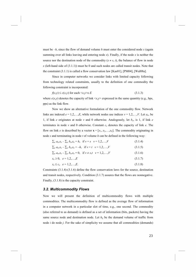
must be –h, since the flow of demand volume h must enter the considered node x (again
summing over all links leaving and entering node x). Finally, if the node x is neither the
source nor the destination node of the commodity (x ≠ s, t), the balance of flow in node
x (left-hand side of (3.1.1)) must be 0 and such nodes are called transit nodes. Note that
the constraint (3.1.1) is called a flow conservation law [Kas01], [PM04], [Wal08a].
Since in computer networks we consider links with limited capacity following
from technology related constraints, usually to the definition of one commodity the
following constraint is incorporated:
f(x,y) ≤ c(x,y) for each <x,y>∈E (3.1.3)
where c(x,y) denotes the capacity of link <x,y> expressed in the same quantity (e.g., bps,
pps) as the link flow.
Now we show an alternative formulation of the one commodity flow. Network
links are indexed e = 1,2,…,E, while network nodes use indices v = 1,2,…,V. Let aev be
1, if link e originates at node v and 0 otherwise. Analogously, let bev is 1, if link e
terminates in node v and 0 otherwise. Constant ce denotes the capacity of link e. The
flow on link e is described by a vector x = [x1, x2,…,xE]. The commodity originating in
node s and terminating in node t of volume h can be defined in the following way:
∑e aevxe – ∑e bevxe = h, if v = s v = 1,2,…,V (3.1.4)
∑e aevxe – ∑e bevxe = –h, if v = t v = 1,2,…,V (3.1.5)
∑e aevxe – ∑e bevxe = 0, if v ≠ s,t v = 1,2,…,V (3.1.6)
xe ≥ 0, e = 1,2,…,E (3.1.7)
xe ≤ ce e = 1,2,…,E. (3.1.8)
Constraints (3.1.4)-(3.1.6) define the flow conservation laws for the source, destination
and transit nodes, respectively. Condition (3.1.7) assures that the flows are nonnegative.
Finally, (3.1.8) is the capacity constraint.
3.2. Multicommodity Flows
Now we will present the definition of multicommodity flows with multiple
commodities. The multicommodity flow is defined as the average flow of information
in a computer network in a particular slot of time, e.g., one second. The commodity
(also referred to as demand) is defined as a set of information (bits, packets) having the
same source node and destination node. Let hij be the demand volume of traffic from
node i do node j. For the sake of simplicity we assume that all commodities (demands)
23

are numbered from 1 to D. Let sd and td denote the source and destination of demand d,
respectively. Let hd be the volume of demand d, i.e., hd = hij for i = sd and j = td. There
are two ways to formulate multicommodity flow: node-link notation and link-path
notation. The multicommodity flow formulated using the node-link notation is defined
as functions fd : E → R1 d = 1,2,...,D in the following way:
∑
=−
≠
=
=∑ − ∈∈ )()(
,
,,0
,
),(),( xBy
dd
dd
dd
dxAy d
txh
tsx
sxh
xyfyxf (3.2.1)
fd(x,y) ≥ 0 for each <x,y>∈E. (3.2.2)
Notice that the flow conservation law (3.2.1) is very similar to (3.1.1). The only
difference is the additional lower index d related to demands. fd(x,y) denotes the flow of
commodity d in link <x,y>. For every demand d we check the balance of flow in each
node x (left-hand side of (3.2.1)). In the case of the source node of the particular
demand d (x = sd), the value must be equal to the demand volume hd. In the case of the
destination node (x = td), the right-hand side of (3.2.1) must be –hd. Finally, for all
transit nodes (x ≠ sd, td) the flow balance is 0. Let f(x,y) denote the summary flow in link
<x,y>:
∑==
D
dd yxfyxf
1),(),( . (3.2.3)
Notice that f(x,y) is calculated as a sum of the link flow over all demands. Using the link
flow definition (3.2.3) we can formulate the capacity constraint (i.e., the link flow
cannot exceed the link capacity):
f(x,y) ≤ c(x,y) for each <x,y>∈E. (3.2.4)
Now we present the node-link formulation of multicommodity flows using the
notation proposed in [PM04] that can be also used in this book. We assume that
demands are indexed as d = 1,2,…,D. Variable xed denotes the flow of demand d
allocated to link e.
�ode-Link Formulation
indices
v = 1,2,…,V network nodes
d = 1,2,…,D demands
e = 1,2,…,E network links
24
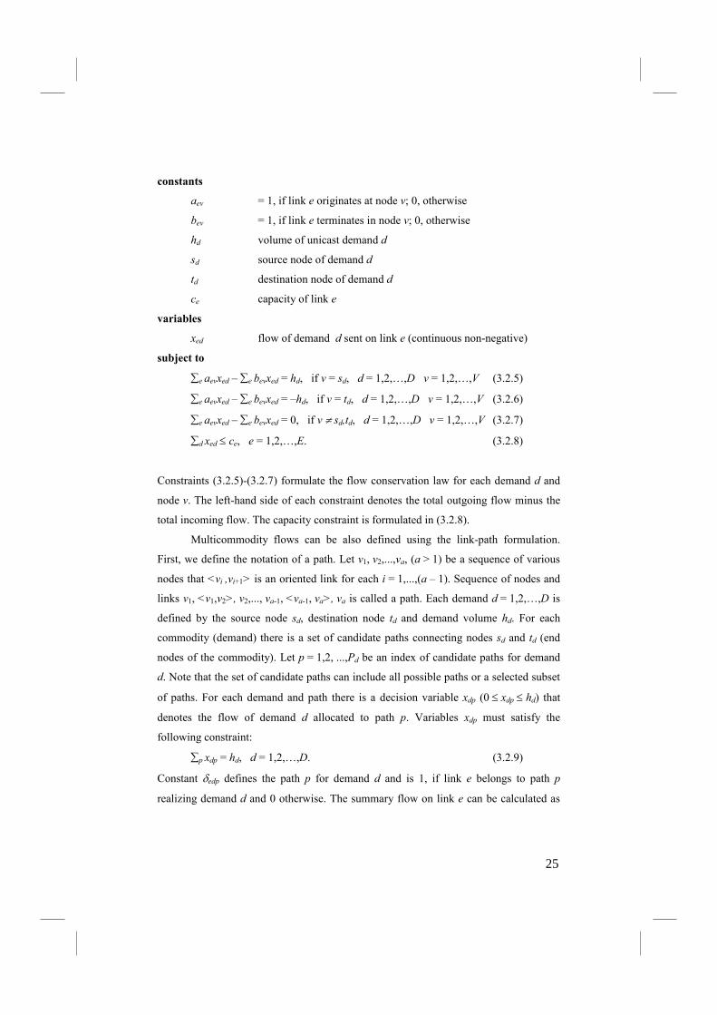
constants
aev = 1, if link e originates at node v; 0, otherwise
bev = 1, if link e terminates in node v; 0, otherwise
hd volume of unicast demand d
sd source node of demand d
td destination node of demand d
ce capacity of link e
variables
xed flow of demand d sent on link e (continuous non-negative)
subject to
∑e aevxed – ∑e bevxed = hd, if v = sd, d = 1,2,…,D v = 1,2,…,V (3.2.5)
∑e aevxed – ∑e bevxed = –hd, if v = td, d = 1,2,…,D v = 1,2,…,V (3.2.6)
∑e aevxed – ∑e bevxed = 0, if v ≠ sd,td, d = 1,2,…,D v = 1,2,…,V (3.2.7)
∑d xed ≤ ce, e = 1,2,…,E. (3.2.8)
Constraints (3.2.5)-(3.2.7) formulate the flow conservation law for each demand d and
node v. The left-hand side of each constraint denotes the total outgoing flow minus the
total incoming flow. The capacity constraint is formulated in (3.2.8).
Multicommodity flows can be also defined using the link-path formulation.
First, we define the notation of a path. Let v1, v2,...,va, (a > 1) be a sequence of various
nodes that <vi ,vi+1> is an oriented link for each i = 1,...,(a – 1). Sequence of nodes and
links v1, <v1,v2>, v2,..., va-1, <va-1, va>, va is called a path. Each demand d = 1,2,…,D is
defined by the source node sd, destination node td and demand volume hd. For each
commodity (demand) there is a set of candidate paths connecting nodes sd and td (end
nodes of the commodity). Let p = 1,2, ...,Pd be an index of candidate paths for demand
d. Note that the set of candidate paths can include all possible paths or a selected subset
of paths. For each demand and path there is a decision variable xdp (0 ≤ xdp ≤ hd) that
denotes the flow of demand d allocated to path p. Variables xdp must satisfy the
following constraint:
∑p xdp = hd, d = 1,2,…,D. (3.2.9)
Constant δedp defines the path p for demand d and is 1, if link e belongs to path p
realizing demand d and 0 otherwise. The summary flow on link e can be calculated as
25
fe = ∑d∑p δedpxdp. Consequently, the capacity constraint for link-path notation is
formulated in the following way:
∑d∑p δedpxdp ≤ ce, e = 1,2,…,E. (3.2.10)
Constraints (3.2.9)-(3.2.10) define multicommodity flows using the link-path notation.
Condition (3.2.9) assures that the whole demand d is sent in the network, i.e., the whole
demand volume hd must be allocated to various candidate paths p = 1,2, ...,Pd. Note that
constraint (3.2.9) is equivalent to the flow conservation law used in the node-link
notation.
Another link-path formulation can be as follows. Let decision variable xdp
(0 ≤ xdp ≤ 1) denote the fraction of demand d flow allocated to path p (not the part of
demand d flow allocated to path p as above). In this case, the formulation is as follows:
∑p xdp = 1, d = 1,2,…,D (3.2.11)
∑d∑p δedpxdphd ≤ ce, e = 1,2,…,E. (3.2.12)
Notice that in this formulation the right-hand side of (3.2.11) is 1. Moreover, the link
flow is calculated as ∑d∑p δedpxdphd (left-hand side of (3.2.12)). For examples related to
modeling of multicommodity flows refer to [PM04].
3.3. Types of Multicommodity Flows
There are two types of multicommodity flows:
• Bifurcated flows. The commodity (demand) can be split and sent using many
different paths, e.g., IP protocol.
• Non-bifurcated (unsplittable, single-path) flows. The whole commodity (demand)
is sent along one path, e.g., connection oriented network techniques (MPLS,
ATM, Frame Relay, WDM).
Now we show how the two types of flows can be formulated using both notations
introduced above. First, we use the link-path formulation. To define bifurcated
multicommodity flows we assume that xdp is a continuous and non-negative variable.
The following two constraints formulate bifurcated multicommodity flows:
∑p xdp = hd, d = 1,2,…,D (3.3.1)
0 ≤ xdp ≤ hd, d = 1,2,…,D p = 1,2,…,Pd. (3.3.2)
In the context of non-bifurcated flows xdp is a binary variable satisfying the
following constraints:
26
∑p xdp = 1, d = 1,2,…,D (3.3.3)
xdp∈{0,1}, d = 1,2,…,D p = 1,2,…,Pd. (3.3.4)
For the node-link formulation bifurcated flows use a continuous and non-
negative variable xed satisfying the following constraints:
∑e aevxed – ∑e bevxed = hd, if v = sd, d = 1,2,…,D v = 1,2,…,V (3.3.5)
∑e aevxed – ∑e bevxed = –hd, if v = td, d = 1,2,…,D v = 1,2,…,V (3.3.6)
∑e aevxed – ∑e bevxed = 0, if v ≠ sd,td, d = 1,2,…,D v = 1,2,…,V (3.3.7)
0 ≤ xed ≤ hd, d = 1,2,…,D e = 1,2,…,E. (3.3.8)
Constraints (3.3.5)-(3.3.7) formulate the flow conservation law. We use notation as in
previous section. Analogously, in the context of non-bifurcated flows xed is a binary
(integer) variable satisfying the following constraints:
∑e aevxed – ∑e bevxed = 1, if v = sd, d = 1,2,…,D v = 1,2,…,V (3.3.9)
∑e aevxed – ∑e bevxed = –1, if v = td, d = 1,2,…,D v = 1,2,…,V (3.3.10)
∑e aevxed – ∑e bevxed = 0, if v ≠ sd,td, d = 1,2,…,D v = 1,2,…,V (3.3.11)
xed∈{0,1}, d = 1,2,…,D e = 1,2,…,E. (3.3.12)
The formulations of multicommodity flows presented above in this section can
be used in context of various objective functions and additional constraints following
from requirements arising in real network technologies. Some examples can be found in
further sections of this book. For more details on multicommodity flows refer to
[Ass78], [PM04], [Kas01].
27
4. Flow Optimization
In this chapter we will focus on flow optimization problems also called flow assignment
(FA) problems. We consider an existing network, which is in an operational phase and
augmenting of its resources (links, capacity) is not possible in a short time perspective.
However, there is a need to improve the network performance and the only possible
way is to change the network routing. Various performance metrics can be considered,
e.g., cost, delay, survivability, etc. Details of the optimization model (e.g., kind of
multicommodity flows, constraints, performance metric) are formulated according to
the considered network technology and customer’s requirements.
In the flow optimization problem, for the given set of demands (described by:
demand volume, origin node, destination node and optionally candidate paths) we want
to select the routing, i.e., determine network paths used for transmission of demands.
The most important constraint is related to the limited link capacity. Since the network
is fixed, the total flow on each link cannot exceed the given physical link capacity.
4.1. Bifurcated Flows with Linear Objective Function
Now we focus on optimization of bifurcated multicommodity flows with linear
objective function. Recall that bifurcated multicommodity flows assume that the
demand between a pair of nodes can be split and sent using multiple paths connecting
this pair of nodes for instance like in IP protocol.
We start with a classical flow allocation problem formulated using the link-path
notation [PM04]. We are given a set of demands denoted by an index d = 1,2,…,D.
Demand volume is given by hd. For each demand d we know a set of candidate paths
p = 1,2,…,Pd connecting the origin and destination node of the demand. The network is
described by a set of links (directed edges) indexed e = 1,2,…,E and link capacity given
by ce. Note that values of demand volume (hd) and link capacity (ce) are expressed in the
same unit, e.g., bits per seconds (bps) or packets per second (pps). Every candidate path
p realizing demand d is defined by a constant δedp which is 1, if link e belongs to path p
of demand d and 0, otherwise. The objective of the bifurcated flow allocation problem
is to find a feasible set of paths to send all demands in the network according the
capacity constraint of each link. The decision variable xdp denotes a flow of demand d
allocated to path p and is continuous and non-negative.
28
Bifurcated Flow Allocation Problem
indices
d = 1,2,…,D demands
p = 1,2,…,Pd candidate paths for demand d
e = 1,2,…,E network links
constants
δedp = 1, if link e belongs to path p realizing demand d; 0, otherwise
hd volume of unicast demand d
ce capacity of link e
variables
xdp flow allocated to path p of demand d (continuous non-negative)
subject to
∑p xdp = hd, d = 1,2,…,D (4.1.1)
∑d∑p δedpxdp ≤ ce, e = 1,2,…,E. (4.1.2)
Since problem (4.1.1)-(4.1.2) is an allocation problem, there is no objective function.
The problem includes only two constraints. The former one (4.1.1) assures that the
whole volume of each demand d is realized in the network. The latter condition (4.1.2)
is a capacity constraint to meet the technological constraint that flow of each link
(called also link load) given as a sum of all demands that uses this link (i.e., ∑d∑p δedp
xdp) cannot exceed the link capacity. Note that it is possible that in some case no feasible
solution exists. The problem is a linear with continuous variables, so the Simplex
method can be used to find optimal solution. If the problem is feasible, then there is a
solution with at most D + E non-zero flows [PM04].
The next example of a bifurcated flow problem has the goal to allocate network
flows in order to minimize the additional link capacity that is required in the network to
allocate flows for all demands. An additional variable z denotes the link additional
capacity.
Modified Bifurcated Flow Allocation Problem
variables (additional)
z additional link capacity (continuous non-negative)
objective
29
minimize z (4.1.3)
subject to
∑p xdp = hd, d = 1,2,…,D (4.1.4)
∑d∑p δedpxdp ≤ ce + z, e = 1,2,…,E. (4.1.5)
Comparing to the previous problem, there is an objective function (4.1.3). Moreover,
the capacity constraint (4.1.5) is changed, since on the right-hand side we add the
variable z. Note that the problem (4.1.1)-(4.1.2) in some case can be not feasible, while
the problem (4.1.3)-(4.1.5) is always feasible. However, if the optimal objective of
(4.1.3)-(4.1.5), z, is non-positive then the corresponding optimal flows xdp determine a
feasible solution for the allocation problem given by (4.1.1)-(4.1.2).
An important challenge of the link-path formulation is the size of optimization
problem, which is a function of the number of candidate paths. Since the number of
candidate paths increases exponentially with the network size, it is almost impossible to
consider all candidate paths in the formulation, even for relatively small networks.
Thus, usually a small subset of all possible candidate paths is considered. However, this
approach does not guarantee to find a global optimum of the flow assignment problem,
since some possible paths are excluded from the pool of candidate paths. One of popular
methods to reduce the number of candidate paths is a hop-limit approach proposed in
[HBU95] for spare capacity assignment. Under this method, the process of reducing the
size of the optimization problem is achieved by taking into account all networks eligible
routes, which do not violate a predetermined hop-limit value. In particular, if for a given
demand the length of the shortest route is n hops and the hop limit is hl, then we
consider all routes which are not longer than (n + hl) hops.
To illustrate the hop-limit approach we demonstrate a simple example [Wal04d].
We calculate the number of routes generated according to the given hop limit for two
families of networks: 10-node (Fig. 4.1) and 36-node (Fig. 4.2). Connectivity of tested
networks is denoted by the average node degree parameter (avnd) calculated as the
number of links divided by the number of nodes. In the case of 10-node topologies, we
consider 4 networks with 34, 38, 42 and 46 links, consequently the corresponding
values of the anvd parameter are 3.4, 3.8, 4.2 and 4.6. In the case of 36-node topologies,
we examine 7 networks having 104, 114, 128, 144, 162, 180 and 200 links and
connectivity expressed by avnd is in the range from 2.88 to 5.56. The y-axis of figures
30

showing the number of routes uses the logarithmical scale. The x-axis represents the
hop limit.
Notice that in the case of 36-node topologies the network with low connectivity
(avnd=2.88) the number of routes with hl=6 is 1.33E+05. For a dense network
(avnd=5.56) the corresponding number of routes is 7.90E+07. Since in the link-path
formulation the number of variables and size of the flow assignment problem depends
on the number of possible routes, even for low-connected networks considering hop
limit greater than 5 is not reasonable for 36-nodes networks. Another important
observation is that the number of routes grows exponentially with the hop limit.
100
1000
10000
100000
0 1 2 3 4 5 6 7
Hop limit
Average number of paths avnd=3.4 avnd=3.8
avnd=4.2 avnd=4.6
Fig. 4.1. The average path number as a function of the hop limit and network connectivity
for 10-node network
1.0E+03
1.0E+04
1.0E+05
1.0E+06
1.0E+07
1.0E+08
1.0E+09
0 1 2 3 4 5 6 7
Hop limit
Average number of paths avnd=2.88 avnd=3.17
avnd=3.56 avnd=4.00
avnd=4.50 avnd=5.00
avnd=5.56
Fig. 4.2. The average path number as a function of the hop limit and network connectivity
for 36-node network
31

Another approach to tackle the issues of the candidate paths number and make
the flow optimization problem manageable is a Column Generation Technique using
Lagrangian relaxation. For more details see [PM04].
4.2. Bifurcated Flows with Convex Objective Function
Flow allocation problems beside linear objective function use also convex functions.
The most important example of a convex function is network delay objective [Kle64],
[FGK73], [Kas01]. The network delay function was formulated by Kleinrock in 1964
[Kle64] in the following way:
∑−
= eee
e
fc
fF
γ1
, (4.2.1)
where γ is the network throughput, fe denotes the flow on link e and ce is the capacity of
link e. The delay function was formulated for store-and-forward networks according to
several assumptions. The most significant is the independence assumption, i.e., each
time that a message is received at a node within the net, a new length is chosen for this
message independently from an exponential distribution. Moreover, each link behaves
as independent M/M/1 queue system regardless of traffic interaction of various
demands. For more details on the network delay function refer to [Kle64], [FGK73],
[Kas01]. Below we formulate a bifurcated flow assignment problem with the delay
objective.
Bifurcated Flow Allocation Delay Problem
indices
d = 1,2,…,D demands
p = 1,2,…,Pd candidate paths for demand d
e = 1,2,…,E network links
constants
δedp = 1, if link e belongs to path p realizing demand d; 0, otherwise
hd volume of unicast demand d
ce capacity of link e
γ throughput
variables
xdp flow allocated to path p of demand d (continuous non-negative)
fe flow on link e (continuous non-negative)
32

objective
minimize F = 1 / γ ∑e fe / (fe – ce) (4.2.2)
subject to
∑p xdp = hd, d = 1,2,…,D (4.2.3)
fe = ∑d∑p δedpxdp, e = 1,2,…,E. (4.2.4)
fe ≤ ce, e = 1,2,…,E. (4.2.5)
The objective (4.2.2) is the network delay function. Comparing to previous models
formulated above, we introduce an auxiliary variable fe that denotes the flow (load) on
link e (4.2.4). fe is calculated as sum over all demands d = 1,2,…,D and all candidate
paths p = 1,2,…,Pd taking into account the amount of demand d allocated to path p (xdp)
and checking if a particular path uses link e (δedp = 1). Since the objective (4.2.2) is
nonlinear (convex) the problem cannot be solved using the Simplex method. The
possible solution methods include: direct methods (FD (Flow Deviation) [FGK73] GP
(Gradient Projection) [PM04], EF (Extremal Flows) [CG74]); linear approximation of
the convex function using a set of linear functions and next the application of linear
programming algorithms, e.g., Simplex; other heuristics (e.g., evolutionary algorithm).
Now we introduce the Flow Deviation algorithm proposed in [FGK73]. Let
f = [f1,f2,…,fE] denote a vector of feasible bifurcated multicommodity flows in all links
e = 1,2,…,E. Let us assume that P(f) is a convex objective function (e.g., network delay
function (4.2.1). The FD operator which maps a flow f into another flow is defined in
the following way:
FD(v,λ) � f = (1 – λ)f + λv (4.2.6)
where v is a shortest route flow under metric le = ∂P / ∂fe, which is partial derivative of
function P. λ is a step size that minimizes P[(1 – λ)f + λv], where (0 ≤ λ ≤ 1). Note that
the goal of the FD operator (4.2.6) is to deviate a part of the flows (given by λ) to
shortest paths.
In the context of the delay function the link metric (partial derivative of delay
function (4.2.1) is calculated as:
2)(
1
ee
ee
fc
fl
−=
γ (4.2.7)
33
Algorithm Flow Deviation for Bifurcated Flows [FGK73]
Phase 1:
Step 0. With RE0 = 1, let f0 be the shortest flow computed at f = 0. Let n = 0.
Step 1. Let e
ne
Een
c
f
,...,2,1max
==σ . If σn / REn < 1, let f
0 = fn / REn and go to Phase 2.
Otherwise, let REn+1 = REn(1 – ε |1 – σn|) / σn, where ε is a proper tolerance,
0 < ε < 1. Let gn+1 = fn(REn+1 / REn). Go to 2.
Step 2. Let fn+1 = FD � gn+1.
Step 3. If n = 0, go to 5.
Step 4. If |∑e le(ve – gen+1)| < θ and |REn+1 – REn| < δ, where θ and δ are proper positive
tolerances, v is the shortest route computed at gn+1, stop: the problem is
infeasible within tolerances θ and δ. Otherwise go to 5.
Step 5. Let n = n + 1 and go to 1.
Phase 2:
Step 0. Let n = 0.
Step 1. fn+1 = FD � fn.
Step 2. If |∑e le(ve – fen)| < θ, where θ is a proper positive tolerances, stop: fn is optimal
within tolerance θ. Otherwise, let n = n + 1 and go to 1.
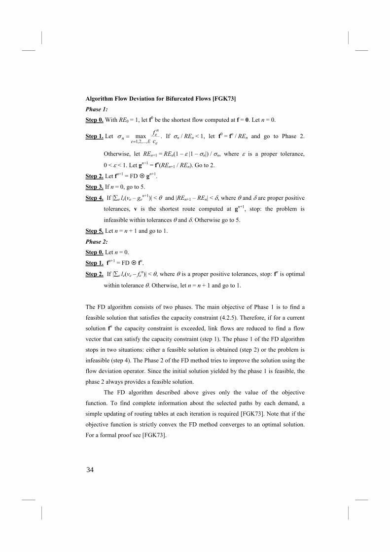
The FD algorithm consists of two phases. The main objective of Phase 1 is to find a
feasible solution that satisfies the capacity constraint (4.2.5). Therefore, if for a current
solution fn the capacity constraint is exceeded, link flows are reduced to find a flow
vector that can satisfy the capacity constraint (step 1). The phase 1 of the FD algorithm
stops in two situations: either a feasible solution is obtained (step 2) or the problem is
infeasible (step 4). The Phase 2 of the FD method tries to improve the solution using the
flow deviation operator. Since the initial solution yielded by the phase 1 is feasible, the
phase 2 always provides a feasible solution.
The FD algorithm described above gives only the value of the objective
function. To find complete information about the selected paths by each demand, a
simple updating of routing tables at each iteration is required [FGK73]. Note that if the
objective function is strictly convex the FD method converges to an optimal solution.
For a formal proof see [FGK73].
34
Another solution method for convex flow assignment problems is linear
approximation of the convex function, i.e., the convex function is approximated by a
piecewise linear function. Let us formulate a set of functions that establish a linear
approximation of a convex function f(z) in the following way:
fk(z) = akz + bk, sk-1 ≤ z < sk. k = 1,2,…,K (4.2.8)
Note that the function f(z) is approximated using k = 1,2,…,K ranges of the
argument z. Due to convexity of the f(z) function, the following condition holds:
f(z) = max k = 1,2,…,K {akz + bk}.
Therefore, the convex function optimization problem can be substituted by a
following problem.
Linear Approximation Convex Function Problem
objective
minimize r = f(y)
constraints
r ≥ aky + bk, k = 1,2,…,K.
For more details on the linear approximation of convex functions refer to [PM04].
4.3. Non-bifurcated Flows
Many network protocols and technologies are connection oriented, e.g., MPLS,
DWDM, ATM [PER05]. To model connection flows the non-bifurcated
multicommodity flows must be applied, i.e., each demand uses only a single path. First,
we formulate a non-bifurcated flow allocation problem equivalent to (4.1.1)-(4.1.2).
�on-bifurcated Flow Allocation Problem
indices
d = 1,2,…,D demands
p = 1,2,…,Pd candidate paths for demand d
e = 1,2,…,E network links
constants
δedp = 1, if link e belongs to path p realizing demand d; 0, otherwise
hd volume of unicast demand d
ce capacity of link e
35
variables
xdp = 1, if path p is used to realize demand d; 0, otherwise (binary)
subject to
∑p xdp = 1, d = 1,2,…,D (4.3.1)
∑d∑p δedpxdphd ≤ ce, e = 1,2,…,E. (4.3.2)
Comparing the non-bifurcated problem (4.3.1)-(4.3.2) to the bifurcated version (4.1.1)-
(4.1.2), we can notice the following differences. For every demand d the sum over p of
binary variables xdp must be 1. In this way, the single path routing is guaranteed. Since
the decision variable xdp is binary, the left-hand side of (4.3.2) includes the demand
volume hd. The above problem is integer (binary), linear and NP-complete [PM04].
Therefore, to find an optimal solution a branch and bound or branch and cut algorithm
must be applied. But, due to complexity of the problem, only for relatively small
networks (10-20 nodes) the optimal solution can be found in reasonable time. The
heuristic algorithms can be applied to obtain a suboptimal solution for larger networks.
Note that non-bifurcated flow assignment problems face the same problem of candidate
paths number as bifurcated flow problems, for more details see Section 4.1.
The network delay problem in the context of non-bifurcated flows is formulated
as follows.
�on-bifurcated Flow Allocation Delay Problem
indices
d = 1,2,…,D demands
p = 1,2,…,Pd candidate paths for demand d
e = 1,2,…,E network links
constants
δedp = 1, if link e belongs to path p realizing demand d; 0, otherwise
hd volume of unicast demand d
ce capacity of link e
γ throughput
variables
xdp = 1, if path p is used to realize demand d; 0, otherwise (binary)
fe flow on link e (continuous non-negative)
36
objective
minimize F = 1 / γ ∑e fe / (fe – ce) (4.3.3)
subject to
∑p xdp = 1, d = 1,2,…,D (4.3.4)
fe = ∑d∑p δedpxdphd, e = 1,2,…,E. (4.3.5)
fe ≤ ce, e = 1,2,…,E. (4.3.6)
The above problem is integer (binary), linear and NP-complete [PM04]. Below we
present several algorithms for this problem.
We start with a FD method for non-bifurcated flows [FGK73]. To find a
feasible, initial solution algorithm similar to the phase 1 of bifurcated FD (see the
previous section) can be used. Let set X (called selection) include all variables xdp that
are equal to 1. Selection X determines the unique set of currently selected paths for each
demand and in consequence the link flow defined in (4.3.5). Operator first(B) returns
the index of the first demand in set B. G and H are selections. Let F(H) denote the delay
function (4.3.3) for a feasible selection H.
Algorithm Flow Deviation for �on-bifurcated Flows [FGK73]
Step 1. Find feasible selection X1. Set r = 1, and go to 2.
Step 2. Compute SR(Xr), defined as the set of shortest routes under metric le (4.2.7) for
each demand d.
Step 3. Set H = Xr and let K be a set of all demands.
a) Find d = first(K). Set G = (H – {xdk}) ∪ {xdi}, where xdk∈H and xdi∈SR(Xr).
b) If F is a feasible selection and F(G) < F(H), let H = G.
c) Set K = K – {d}. If K = ∅, go to 4. Otherwise, go to 3a.
Step 4. If H = Xr, stop. The algorithm cannot improve the solution any further.
Otherwise, let Xr+1 = H, r = r + 1 and go to 2.
The main idea of the non-bifurcated FD algorithm is as follows. We start with a feasible
(in terms of the capacity constraint and single path routing) solution X1 and the
algorithm tries to improve the solution. For each considered selection Xr of path
variables, we calculate a selection SR(Xr) containing the shortest paths according to the
le metric (4.2.7), which is the partial derivative of the delay function (4.3.3). Next, we
37

try to improve the solution by deviation of one selected connection to another route
(Step 3). If the switch to a shortest path of the considered demand d (Step 3a) provides a
feasible solution (i.e., the capacity constraint (4.3.6) is satisfied) and reduces the
objective function (4.3.3), the new selection is saved (step 3b). The algorithm converges
in a finite number of steps, since there are a finite number of non-bifurcated flows.
Repetitions of the same flow are impossible due to the stopping condition (Step 4). Note
that the non-bifurcated FD algorithm can be modified to be applied in the context of
other objective functions, e.g., see [BOK03], [Wal03d], [Wal04a], [Wal06a].
Computational intelligence provides a wide range of effective algorithms that
can be applied to various optimization problems. Now we focus on evolutionary
algorithms (EA) that are search procedures, which try to simulate mechanics of natural
selection and natural genetics. A variety of problems can be coded into a chromosome
that together with a fitness function makes individual, which are organized into
populations. From the current population, the population is evolved to a new population
using three operators: reproduction, crossover, mutation. For more details on
evolutionary algorithms refer to [Gol89], [MIT98].
We show how to use an evolutionary algorithm (EA) to solve problem (4.3.3)-
(4.3.6). The initial step to design an evolutionary algorithm is to code the considered
problem into chromosomes. In our approach the chromosome has as many alleles as
demands in the network. Each allele represents the index of a selected path (variables
xdp). For example, the following chromosome cr=213 means that demand d = 1 uses
path p = 2, demand d = 2 selects path p = 1 and demand d = 3 applies path p = 3. Thus,
the following variables are equal to 1: x12, x21 and x33. All remaining variables are equal
to 0. Consequently, each chromosome is equivalent to the selection and enables to
calculate link flow (4.3.5) and objective function (4.3.3). Another important issue that
must be addressed to develop an evolutionary algorithm is the fitness function, which
should return a non-negative value that is to be maximized. Moreover, the EA algorithm
solves problems without constraints. If the considered optimization problem has
constraints (as in the case of the (4.3.3)-(4.3.6) problem), there are two ways to
construct the evolutionary algorithm. First, the selected chromosome coding can include
the constraints. For instance, in our case constraint (4.3.4) is included in the
chromosome. Second, a penalty function approach can be applied, i.e., the fitness
function contains not only the objective function, but also a special term including a
measure of violation of the constraints scaled by a penalty parameter. It is assumed that
38
the measure of violation is nonzero, if the constraint is violated and is zero in the region
where the constraint is not exceeded. Let F(cr) return the value the objective function
(4.3.3) of solution coded in the chromosome cr. Let FPEN(cr) denote the value of the
delay function (4.3.3) with additional penalty function for chromosome cr:
FPEN(cr) = F(cr) + P6∑eH(cr,e) (4.3.7)
where H(cr,e) denotes the violation of capacity constraint (4.3.6) according to network
flows given by cr. If the capacity constraint is not violated (i.e., fe ≤ ce), then
H(cr,e) = 0. Otherwise, we set H(cr,e) = fe – ce. P6 is a penalty parameter that scales the
penalty function. Fitness function is defined as follows:
Fitness(cr) = M(FMAX – FPEN(cr) ) (4.3.8)
where FMAX denotes the maximum value the F
PEN(cr) taking into account all
chromosomes cr in a given population. M is a scaling parameter that enables to make
additional tuning of the algorithm.
For the proposed coding and fitness function formulation, classical crossover
and mutation operators can be used. The only required modification is to assure that the
operator yields a feasible solution, i.e., the value of the new allele for demand d cannot
exceed the number of candidate paths given by Pd [Wal01a].
Also other computational intelligence and stochastic methods can be applied to
flow optimization, e.g., ant algorithm [Wal01b], [Wal04c]; tabu search [PM04]; local
search [PM04]; simulated annealing [PM04].
To find an optimal solution of a non-bifurcated flow assignment problem, a
branch and bound algorithm must be applied. Below we present a framework of an
algorithm that can be applied to a wide range of non-bifurcated flow problems [BK83],
[Wal04b]. Let Ur and Tr be sets of decision variables xdp constantly and momentarily
fixed in the r-th iteration, respectively. Let F(Xr) denote the value of the objective
function (e.g., network delay) for the selection Xr. F* denotes the best already found
solution, LBr is a lower bound of a selection Xr. Let X1 include the initial, feasible
solution. Let U1 = ∅, T1 = ∅, F* = ∞ and r = 1.
Algorithm Branch and Bound for �on-bifurcated Flows [BK83]
Step 1. If for at least one link e, the fixed flow exceeds the capacity, go to 5.
Otherwise, find the lower bound LBr. If LBr ≥ F* go to 5. Otherwise, go to 2.
39
Step 2. If there is at least one link e that fe > ce, go to 4. Otherwise, find F(Xr). If
F(Xr) < F*, then set F* = F(Xr).
Step 3. If there are not any variables for the choice operation go to 5. Otherwise, choose
the normal variable xdk and a reverse variable xdi. Next generate selection
Xs = (Xr – {xdk}) ∪ {xdi}, Us = Ur ∪ {xdi}, Ts = Tr. Go to 1.
Step 4. If there are not any variables for the choice operation go to 5. Otherwise, choose
the normal variable xdk and a reverse variable xdi. Next generate selection
Xs = (Xr – {xdk}) ∪ {xdi}, Us = Ur ∪ {xdi}, Ts = Tr. Go to 1.
Step 5. Backtrack to the predecessor Xp of the selection Xr. If Xr has no predecessor,
then stop the algorithm. The selection X* associated with the current solution F*
is optimal. Otherwise, update the current selection Xp in the following way. If Xr
has been generated by the reverse variable xdi, set Tp = Tp ∪ {xdi}. If the
backtracking is performed for (Pd – 1) time by a reverse variable of the normal
variable xdk, then Up = Up ∪ {xdk}, Tp = Tp – {xdp : p = 1,2,…,Pd}. Go to 1.
In the proposed branch and bound algorithm we start with a selection X1 and generate a
sequence of selections Xr. In order to obtain the initial selection X1, we must solve the
problem using heuristic algorithms, e.g. FD. Each new selection Xs is obtained from a
certain selection Xr of the sequence by complementing a normal variable xdk by a
reverse variable xdi in the following way Xs = (Xr – {xdk}) ∪ {xdi}. Both variables
(normal and reverse) must be associated with the same demand d in order to satisfy the
condition (4.3.4). The generating process can be represented as a branch and bound
decision tree. Each node of the decision tree represents one selection. Each arc of the
tree represents a pair of selections (Xr, Xs) such that Xs is obtained from Xr. We say that
the selection Xs is a successor of the selection Xr, if there is a path from Xr to Xs. For
every selection Xr we constantly fix a subset Ur∈Xr and momentarily fix a set Tr. The
variables in Ur are constantly fixed and denote the path from the initial selection X1 to
the current selection Xr in the branch and bound decision tree. Each momentarily fixed
variable in Tr is the variable abandoned during the backtracking process. There are two
important elements of the branch and bound algorithm that are calculated for each
selection Xr: the lower bound of the criterion function and the branching rules. The
lower bound is calculated to check if a better solution (with lower objective function
value) may be found. If the testing is negative we abandon the considered selection Xr
40
and backtrack to the selection Xp from which the selection Xr was generated. The basic
task of the branching rules is to find the variables for complementing to generate a new
selection with the least possible value of the criterion function [Wal04b].
In the context of the (4.3.3)-(4.3.6) problem to find the lower bound we can
apply the bifurcated FD algorithm for each current selection taking into account
constantly and momentarily fixed variables. To relax the problem, we drop the single
routing constraint and assume bifurcated flows. Since the objective is strictly convex,
the bifurcated FD provides an optimal solution. Another method to obtain lower bound
is to use Kuhn-Tucker conditions [BK83].
Now we present a proposal of a choice operation to select normal and reverse
variables. Let lr(d,p) denote the length of path p for demand d calculated using le metric
defined in (4.2.7) under selection Xr:
lr(d,p) = ∑e δedple, d = 1,2,…,D p = 1,2,…,Pd. (4.3.9)
Theorem 4.1 [BK83]
If selection Xs is a successor of Xr obtained in following way Xs = (Xr – {xdk}) ∪ {xdi},
then:
F(Xs) ≥ F(Xr) – ∆rdki (4.3.10)
Where:
∆rdki = hd(l(d,i) – l(d,k)). (4.3.11)
Note that a formal proof of the Theorem 4.1 can be found in [BK83]. According to
Theorem 4.1, ∆rdki estimates the value of the objective function reduction obtained by
generating a new selection. Therefore, if in the current selection Xr we select normal
variable xdk and reverse variable xdi with maximum value of ∆rdki we can guarantee the
largest decrease of the delay function in the successor of the current selection Xr
[BK83].
4.4. Non-bifurcated Congestion Problem
The congestion problem arises in many practical applications encountered in computer
networks. In this section we address a special version of the congestion problem for
non-bifurcated flows. The goal is to maximize the minimum residual capacity of
network links. The residual capacity is defined as the difference between link capacity
41

and link flow and denotes the link capacity, which is not currently used. Another
objective – comparable to the congestion – is the relative congestion defined as
maximum value of the (residual capacity)/capacity ratio over all links in the network.
The congestion problem is also referred in the literature as unsplittable flow problem
(UFP) [BG95], [Bie02], [CFZ94], [DVM94], [KS97], [KS02], [Wal05e]. We formulate
the congestion problem in the following way.
�on-bifurcated Congestion Problem
indices
d = 1,2,…,D demands
p = 1,2,…,Pd candidate paths for demand d
e = 1,2,…,E network links
constants
δedp = 1, if link e belongs to path p realizing demand d; 0, otherwise
hd volume of unicast demand d
ce capacity of link e
variables
xdp = 1, if path p is used to realize demand d; 0, otherwise (binary)
z congestion, i.e., link residual capacity (continuous non-negative)
objective
maximize F = z (4.4.1)
subject to
∑p xdp = 1, d = 1,2,…,D (4.4.2)
fe = ∑d∑p δedpxdphd, e = 1,2,…,E (4.4.3)
z ≤ ce – fe, e = 1,2,…,E. (4.4.4)
Constraint (4.4.4) defines the additional variable z as a minimum value of the link
residual capacity over all links e = 1,2,…,E. Note that condition (4.4.4.) is a link
capacity constraint formulation and if z ≥ 0, the problem is feasible, i.e., link capacity
constraint is satisfied.
To solve the (4.4.1)-(4.4.4) we present a heuristic algorithm proposed in
[Wal05e]. For the sake of simplicity we define the residual capacity of link e in the
following way:
42
ze = ce – fe, e = 1,2,…,E. (4.4.5)
As in previous section, we assume that X is a set (selection) of variables xdp,
which are equal to one. Let X1 denote a feasible initial solution for instance calculated
by the phase 1 of the Non-bifurcated FD algorithm [FGK73]. Let z(H) denote a value of
the link residual capacity obtained for selected paths included selection H. In the
algorithm we use two tuning parameters. First parameter α, is used to define α-
congested links that satisfy the following condition:
ze ≤ (zmin + α(zmax – zmin)) (4.4.6)
where zmin = mine ze is the minimum value of residual capacity and zmax = maxe ze is the
maximal value of residual capacity calculated according to the current selection. All α-
congested links included in set Cong(α). The α parameter enables us to calibrate the
size of Cong(α) set. Note that if α = 1, all links are included in the set Cong(α). If
α = 0.1, only link for which the residual capacity is between zmin and (0.9zmin + 0.1zmax)
are included in Cong(α). The second tuning parameter rmax denotes the number of
algorithms’ iterations.
Algorithm Congestion Avoidance (CA) [Wal05e]
Step 0. Find feasible selection X1. Set r = 1, and go to 1.
Step 1. For a selection Xr find set Cong(α) that includes all α-congested links e that
satisfy condition (4.4.6). Next, let Dcong be a set that includes all demands for
which the selected path uses at least one link included in Cong(α).
Step 2. Find a selection SWP(Xr) of variables xdp associated with the widest-shortest
route p for a selection Xr. To find a widest-shortest route for each demand d first
prune the demand from the network, and next using the SWP algorithm calculate
the path. Set d = 1 and go to 3.
Step 3. Let H = Xr.
a) If d∈Dcong then calculate a selection G from the selection H in the following
way G = (H – {xdk}) ∪ {xdi}, where xdk∈H and xdi∈SWP(Xr). Paths of other
demands except d remain unchanged. Otherwise if, d∉Dcong go to 3c.
b) If z(G) ≥ z(H), then set H = G.
c) If d = D, go to 4. Otherwise, set d = d + 1 and go to 3a.
Step 4. If r ≥ rmax, stop the algorithm. Otherwise, set r = r + 1, Xr = H and go to 1.
43
The idea behind the algorithm is as follows. We start with a feasible solution X1, which
defines all paths used by demands. Consequently, having these paths and demand
volume, the flow and residual capacity of each link can be calculated. To find all α-
congested links we first find the minimal and maximal values of the residual capacity
denoted as zmin and zmax, respectively. In step 1 the Cong(α) set is applied to calculate
set Dcong that includes all demands for which the selected path uses at least one α-
congested link. The motivation behind parameter α is to concentrate on the most
congested arcs and try to increase the residual capacity of arcs included in Cong(α) by
changing paths for demands included in Pcong. To improve the solution, we find a set
SWP(Xr) that comprises new paths for each demand d∈Dcong using the shortest-widest
path (SWP) algorithm (step 2). For more information on the SWP algorithm refer to
[MS97], [WC96]. In particular, for each d∈Dcong we remove the demand d from the
network (i.e., decrease the flow on each link used by the demand d by the demand
volume) and calculate a new path using the SWP algorithm. Next, we try to improve the
solution by deviation of one selected demand d∈Dcong to the widest route (step 3a). In
step 3b we evaluate the new solution denoted as G. If the solution is improved (i.e., the
minimal residual capacity of G is greater or equal to the minimal residual capacity of
the previous selection), we accept the new path for demand d. Note that in Non-
bifurcated FD (Section 4.3) the algorithm solution is compared using condition “less”
(“less” because the problem is to minimize objective function, in our case we want to
maximize the objective function). We use the “greater or equal” condition to enlarge the
solution space analyzed by the algorithm. Moreover, another difference between FD and
CA is the stopping condition. The FD stops if the solution (flow) is not changed after
the deviation. Since we apply the “greater or equal”, we have to change the stopping
condition and repeat the main loop of CA rmax times. For more details and result see
[Wal05e] and [Wal08a].
4.5. Example
In the example we consider the Modified Bifurcated Flow Allocation Problem defined
by (4.1.3)-(4.1.5). We will show how to construct to whole model for an example
network presented in Fig. 4.3. The network has four nodes located in Polish cities:
Szczecin (node 1), Gdańsk (node 2), Wrocław (node 3) and Warszawa (node 4). There
are 5 connections between the cities what gives 10 links (directed edges) in total. To
44

make the example more clear we do not use the index e to number the links, but each
link is described by indices of the two connecting nodes, e.g., link connecting nodes 1
(Szczecin) and node 2 (Gdańsk) has the index 12.
1
2
3
4
3
5
2
5
4
Fig. 4.3. Topology of the example network
The link capacity is as follows:
• Szczecin – Gdańsk: c12 = 3 Mbps, c21 = 3 Mbps;
• Szczecin – Wrocław: c13 = 5 Mbps, c31 = 5 Mbps;
• Gdańsk – Wrocław: c23 = 2 Mbps, c32 = 2 Mbps;
• Gdańsk – Warszawa: c24 = 5 Mbps, c42 = 5 Mbps;
• Wrocław – Warszawa: c34 = 4 Mbps, c43 = 4 Mbps.
We assume that the following three demands are to be established in the
network. Again for the sake of simplicity we use three letters x, y and v to describe the
demands:
• Demand x from Szczecin (node 1) to Warszawa (node 4), demand volume hx;
• Demand y from Gdańsk (node 2) to Wrocław (node 3), demand volume hy;
• Demand v from Wrocław (node 3) to Warszawa (node 4), demand volume hv.
First we will present the modeling using the link-path notation. For each demand we are
given the following candidate paths described as a list of nodes included in the path:
45

• Demand x has four paths:
o {1,2,4} variable x1;
o {1,3,4} variable x2;
o {1,2,3,4} variable x3;
o {1,3,2,4} variable x4;
• Demand y has three paths:
o {2,3} variable y1;
o {2,1,3} variable y2;
o {2,4,3} variable y3;
• Demand v has three paths:
o {3,4} variable v1;
o {3,2,4} variable v2;
o {3,1,2,4} variable v3.
Now we can write the demand constraints (4.1.4) for all three demands:
• Demand x: x1 + x2 + x3 + x4 = hx ;
• Demand y: y1 + y2 + y3 = hy;
• Demand v: v1 + v2 + v3 = hv.
Recall that in the considered model there is also the objective variable z denoting
the additional link capacity (4.1.3). Next we formulate the capacity constraints for all 10
links taking into account the candidate paths presented above:
• Link 12: x1 + x3 + v3 – z ≤ 3;
• Link 21: y2 – z ≤ 3;
• Link 13: x2 + x4 + y2 – z ≤ 5;
• Link 31: v3 – z ≤ 5;
• Link 23: x3 + y1 – z ≤ 2;
• Link 32: x4 + v2 – z ≤ 2;
• Link 24: x1 + x4 + y3 + v2 + v3 – z ≤ 5;
• Link 42: – z ≤ 5;
• Link 34: x2 + x3 + v1 – z ≤ 4;
• Link 43: y3 – z ≤ 4.
Let assume bifurcated flows and the following values of demands: hx = 3 Mbps,
hy = 3 Mbps, hv = 3 Mbps. The CPLEX code of the example for these assumptions is
46
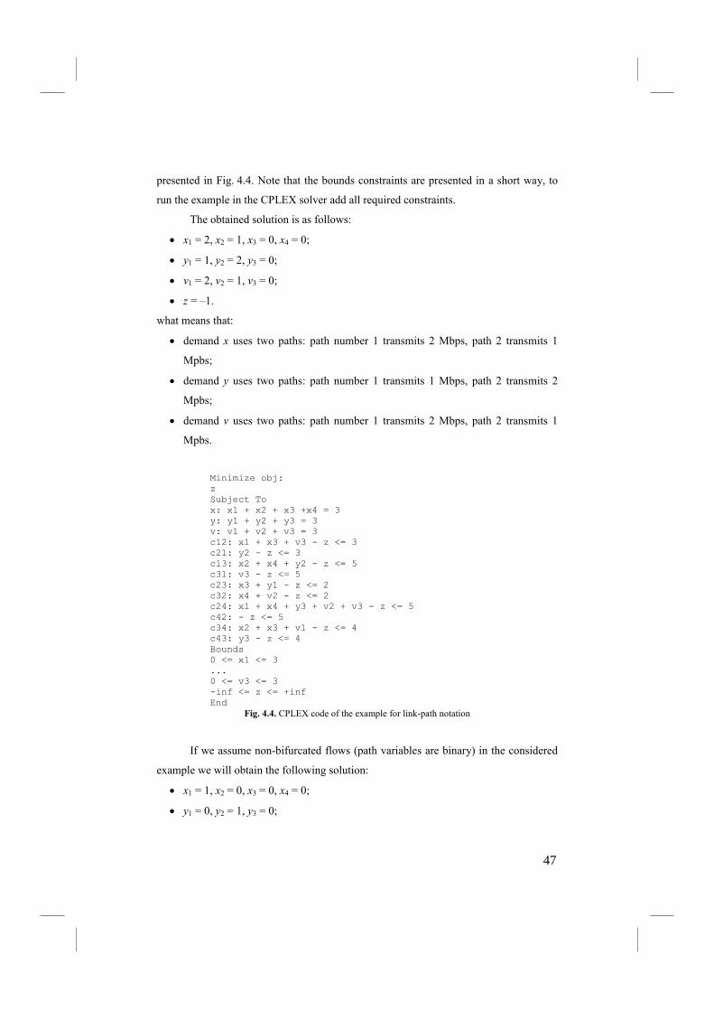
presented in Fig. 4.4. Note that the bounds constraints are presented in a short way, to
run the example in the CPLEX solver add all required constraints.
The obtained solution is as follows:
• x1 = 2, x2 = 1, x3 = 0, x4 = 0;
• y1 = 1, y2 = 2, y3 = 0;
• v1 = 2, v2 = 1, v3 = 0;
• z = –1.
what means that:
• demand x uses two paths: path number 1 transmits 2 Mbps, path 2 transmits 1
Mpbs;
• demand y uses two paths: path number 1 transmits 1 Mbps, path 2 transmits 2
Mpbs;
• demand v uses two paths: path number 1 transmits 2 Mbps, path 2 transmits 1
Mpbs.
Minimize obj:
z Subject To
x: x1 + x2 + x3 +x4 = 3 y: y1 + y2 + y3 = 3 v: v1 + v2 + v3 = 3
c12: x1 + x3 + v3 - z <= 3 c21: y2 - z <= 3
c13: x2 + x4 + y2 - z <= 5 c31: v3 - z <= 5 c23: x3 + y1 - z <= 2
c32: x4 + v2 - z <= 2 c24: x1 + x4 + y3 + v2 + v3 - z <= 5
c42: - z <= 5 c34: x2 + x3 + v1 - z <= 4 c43: y3 - z <= 4
Bounds 0 <= x1 <= 3
... 0 <= v3 <= 3 -inf <= z <= +inf
End
Fig. 4.4. CPLEX code of the example for link-path notation
If we assume non-bifurcated flows (path variables are binary) in the considered
example we will obtain the following solution:
• x1 = 1, x2 = 0, x3 = 0, x4 = 0;
• y1 = 0, y2 = 1, y3 = 0;
47

• v1 = 1, v2 = 0, v3 = 0;
• z = 0.
what means that:
• demand x is sent along path number 1;
• demand y is sent along path number 2;
• demand v is sent along path number 3.
Now we show how to model the example problem using the node-link
formulation (see Chapter 3 for more details on this kind of notation). Let xab, yab and vab
denote the flow of demand x, y and v, respectively for a link between nodes a and b. The
flow conservation law for demand x and each node in the network is written as follows:
• Node 1: x12 + x13 – x21 – x31 = hx;
• Node 2: x21 + x23 + x24 – x12 – x32 – x42 = 0;
• Node 3: x31 + x32 + x34 – x13 – x23 – x43 = 0;
• Node 4: x42 + x43 – x24 – x34 = –hx.
Let consider the first constraint. The flow of demand x leaving the node 1
(x12 + x13) minus the flow entering this node (x21 + x31) must be equal to hx, since the
node 1 is the origin node of demand x. In analogous way we formulate the flow
conservation constraints in the context of demand y
• Node 1: y12 + y13 – y21 – y31 = 0;
• Node 2: y21 + y23 + y24 – y12 – y32 – y42 = hy;
• Node 3: y31 + y32 + y34 – y13 – y23 – y43 = –hy;
• Node 4: y42 + y43 – y24 – y34 = 0.
and demand v:
• Node 1: v12 + v13 – v21 – v31 = 0;
• Node 2: v21 + v23 + v24 – v12 – v32 – v42 = 0;
• Node 3: v31 + v32 + v34 – v13 – v23 – v43 = hv;
• Node 4: v42 + v43 – v24 – v34 = –hv.
The capacity constraint for each link between nodes a and b with capacity cab
looks as follows:
• Link ab: xab + yab + vab – z ≤ cab
The detailed CPLEX code of the node-link formulation is presented in Fig. 4.6. Note
that the bounds constraints are presented in a short way, to run the example in the
CPLEX solver add all required constraints.
48

Minimize obj:
z Subject To
x_1: x12 + x13 - x21 - x31 = 3 x_2: x21 + x23 + x24 - x12 - x32 - x42 = 0 x_3: x31 + x32 + x34 - x13 - x23 - x43 = 0
x_4: x42 + x43 - x24 - x34 = -3 y_1: y12 + y13 - y21 - y31 = 0
y_2: y21 + y23 + y24 - y12 - y32 - y42 = 3 y_3: y31 + y32 + y34 - y13 - y23 - y43 = -3 y_4: y42 + y43 - y24 - y34 = 0
v_1: v12 + v13 - v21 - v31 = 0 v_2: v21 + v23 + v24 - v12 - v32 - v42 = 0
v_3: v31 + v32 + v34 - v13 - v23 - v43 = 3 v_3: v42 + v43 - v24 - v34 = -3 c12: x12 + y12 + v12 - z <= 3
c21: x21 + y21 + v21 - z <= 3 c13: x13 + y13 + v13 - z <= 5
c31: x31 + y31 + v31 - z <= 5 c23: x23 + y23 + v23 - z <= 2 c32: x32 + y32 + v32 - z <= 2
c24: x24 + y24 + v24 - z <= 5 c42: x42 + y42 + v42 - z <= 5
c34: x34 + y34 + v34 - z <= 4 c43: x43 + y43 + v43 - z <= 4 Bounds
0 <= x12 <= 3 ...
0 <= v43 <= 3 -inf <= z <= +inf End
Fig. 4.6. CPLEX code of the example for node-link notation
4.6. Exercises
4.1. Formulate the Flow Allocation Problem (4.1.1)-(4.1.2) using the link-node notation.
4.2. Formulate the Flow Allocation Problem (4.1.1)-(4.1.2) using the link-node notation
with a additional hop-limit approach set for each demand.
4.3. Formulate the Flow Allocation Problem (4.1.1)-(4.1.2) with an additional constraint
to limit the number of used paths for each demand.
4.4. Modify the FD method for bifurcated flows in such a way that the complete
information of selected paths (routing) is available.
4.5. Modify the phase 1 of the bifurcated FD method for non-bifurcated flows.
4.6. Construct a computational intelligence algorithm for a selected flow optimization
problem.
4.7. Write a formal proof of Theorem 4.1.
4.8. Formulate a Non-bifurcated Relative Congestion problem.
49

4.9. Propose a method to calculate a lower bound for the Non-bifurcated Congestion
Problem.
50
5. Capacity and Flow Optimization
In this section we will introduce and examine several capacity and flow optimization
problems (CFA) also called network design problems. CFA problems are one of the
most frequently encountered problems in network optimization. They are used in the
case when a new network is designed or an existing network is incremented. The main
goal of the optimization is to determine the capacity of network links in order to
transmit all demands in the network. The most common objective function used in
network design problems is the cost defined as the cost of network links. However,
other network performance metrics (e.g., delay, survivability) can be applied. The
capacity constraint guaranteeing that the total flow on each link cannot exceed the
selected link capacity is present in all CFA problems. As in previous section, the
modeling details (e.g., various kinds of multicommodity flows, link cost modeling) are
selected according to a particular network technology and other requirements.
5.1. Bifurcated Flows with Linear Objective Function
In this section we concentrate on network design problems assuming bifurcated
multicommodity flows and linear objective function. In the bifurcated multicommodity
flows each demand can use multiple paths. First, we will formulate a basic network
design problem using the link-path notation [PM04]. We use analogous notation as in
previous section, i.e., for each demand d = 1,2,…,D the demand volume hd and a set of
candidate paths p = 1,2,…,Pd. are defined. Continuous variable xdp is used to denote the
demand routing. There is a set of network links (directed edges) e = 1,2,…,E for which
we must determine the capacity. We assume that the capacity is continuous and variable
ye denotes the amount of capacity allocated to link e. Obviously, link capacity ye and
demand volume use the same unit, e.g., bits per seconds (bps) or packets per second
(pps). The network is designed from the scratch, i.e., there is no capacity allocated to
network links.
Simple Design Problem Link-Path �otation
indices
d = 1,2,…,D demands
p = 1,2,…,Pd candidate paths for demand d
e = 1,2,…,E network links
51
constants
δedp = 1, if link e belongs to path p realizing demand d; 0, otherwise
hd volume of unicast demand d
ξe unit (marginal) cost of link e
variables
xdp flow allocated to path p of demand d (continuous non-negative)
ye capacity of link e (continuous non-negative)
objective
minimize F = ∑e ξeye (5.1.1)
subject to
∑p xdp = hd, d = 1,2,…,D (5.1.2)
∑d∑p δedpxdp ≤ ye, e = 1,2,…,E. (5.1.3)
The objective (5.1.1) is to minimize the total network cost that includes the cost of each
link given by the capacity ye allocated to link e multiplied by the unit cost of link e.
Constraint (5.1.2) is in the model to guarantee that the whole volume of each demand d
is sent in the network. (5.1.3) is a link capacity constraint. The problem is linear with
continuous variables. Since the link capacity variable ye is continuous, for optimal
solution the constraint (5.1.3) is binding, i.e., the link flow must be equal to the link
capacities (otherwise, the objective includes cost of an unused capacity). Therefore, we
can write the objective function (5.1.1) as follows:
F = ∑e ξe ∑d∑p δedpxdp = ∑d∑p xdp∑e ξeδedp = ∑d∑p xdpζdp (5.1.4)
where ζdp = ∑e ξeδedp denotes the length of path p for demand d. Consequently, we can
formulate the following rule [PM04].
Shortest-Path Allocation Rule
For each demand, allocate its entire demand volume to its shortest path, with respect to
links unit costs and candidate path. If there is more than one shortest path for a demand
then the demand volume can be split among the shortest paths in an arbitrary way.
Using the above observation, we can write the Simple Design Problem as
follows.
52
Decoupled Simple Design Problem Link-Path �otation
constants (additional)
ζdp length of path p for demand d
variables
xdp flow allocated to path p of demand d (continuous non-negative)
objective
minimize F = ∑d∑p xdpζdp (5.1.5)
subject to
∑p xdp = hd, d = 1,2,…,D (5.1.6)
The above problem can be solved as a set of independent D subproblems, i.e., for each
demand d we find the shortest path from the candidate list. If there is more then 1
shortest path, the demand can be split and use many such paths.
The next model is equivalent to (5.1.1)-(5.1.3), however we use the node-link
notation. Therefore, we take into account all possible paths (not only candidate paths)
and thus the globally optimal solution can be found.
Simple Design Problem �ode-Link �otation
indices (additional)
v = 1,2,…,V network nodes
constants (additional)
aev = 1, if link e originates at node v; 0, otherwise
bev = 1, if link e terminates in node v; 0, otherwise
sd source node of demand d
td destination node of demand d
variables
xed flow of demand d sent on link e (continuous non-negative)
ye capacity of link e (continuous non-negative)
objective
minimize F = ∑e ξeye (5.1.7)
subject to
∑e aevxed – ∑e bevxed = hd, if v = sd, d = 1,2,…,D v = 1,2,…,V (5.1.8)
∑e aevxed – ∑e bevxed = -hd, if v = td, d = 1,2,…,D v = 1,2,…,V (5.1.9)
53

∑e aevxed – ∑e bevxed = 0, if v ≠ sd,td, d = 1,2,…,D v = 1,2,…,V (5.1.10)
∑d xed ≤ ye, e = 1,2,…,E. (5.1.11)
Constraints (5.1.8)-(5.1.9.10) are used to define the multicommodity flows in the node-
link notation. Note that the Shortest-Path Allocation Rule can be also formulated in the
context of the above problem. However, since all possible paths are considered (not
only a limited set of candidate paths) the shortest path algorithm (e.g., Dijkstra) must be
used to solve the decoupled subproblem.
In Table 5.1 we report the comparison between link-path and node-link
formulations in terms of the number of variables and number of constraints. Note that V
denote number of nodes, P average number of candidate paths, k average number of
adjacent nodes, V′ (≤V) number of demand origin nodes. We can easily notice that the
node-link model requires more variables and constraints. But on the other hand, the
link-path node-link formulation does not provide a global optimum. Moreover, the link-
path model requires additional preprocessing to generate the set of candidate paths
[PM04].
Table 5.1. Model comparison
Formulation Number of variables Number of constraints
Link-path PxV′(V′−1) + 0.5kxV=O(V2) PxV′(V′−1)+0.5kxV=O(V2)
Node-link 0.5kxVxV′(V′−1)x=O(V3) VxV′(V′−1)+0.5kxV=O(V3)
In many cases the existing network needs to be incremented in order to address
to increasing network traffic. Therefore, additional capacity is added to the already
allocated capacity. Below we formulate an example of such problem [PM04].
Incremental Design Problem
constants (additional)
ce capacity of link e
variables
xdp flow allocated to path p of demand d (continuous non-negative)
54
ye additional capacity of link e (continuous non-negative)
objective
minimize F = ∑e ξeye (5.1.12)
subject to
∑p xdp = hd, d = 1,2,…,D (5.1.13)
∑d∑p δedpxdp ≤ ce + ye, e = 1,2,…,E. (5.1.14)
The only modification comparing against model (5.1.1)-(5.1.3) is the link capacity
constraint (5.1.14). The right-hand side of (5.1.14) includes the existing capacity ce as
well as the additional capacity ye. Notice that the value cost of a network designed in
several phases using the incremental approach in most cases is greater than the
corresponding cost of from scratch design. This follows from the obvious observation
that if we design a network from scratch the already invested budget (ξece) can be better
allocated [PM04].
5.2. Routing Restrictions
In the previous section we introduced basic formulations of the network design problem
with the bifurcated flows. Now we enhance the models with additional constraints
related to routing of demands and following from network technologies and other
requirements (e.g., financial, reliability, etc.). First, we present a model where each
demand must be provided with path diversity and the flow is sent using more than one
path [PM04]. This constraint may be a consequence of reliability constraints, to
minimize the results of a network failure that in this case affects not the whole demand
but only a part. The diversity factor nd is used to define the maximum portion of the
demand volume (i.e., hd / nd) that can be sent on one path. We use the link-path notation
and bifurcated flows.
Path Diversity Design Problem
indices
d = 1,2,…,D demands
p = 1,2,…,Pd candidate paths for demand d
e = 1,2,…,E network links
constants
55
δedp = 1, if link e belongs to path p realizing demand d; 0, otherwise
hd volume of unicast demand d
ξe unit (marginal) cost of link e
nd diversity factor for demand d
variables
xdp flow allocated to path p of demand d (continuous non-negative)
ye capacity of link e (continuous non-negative)
objective
minimize F = ∑e ξeye (5.2.1)
subject to
∑p xdp = hd, d = 1,2,…,D (5.2.2)
∑d∑p δedpxdp ≤ ye, e = 1,2,…,E. (5.2.3)
xdp ≤ hd / nd, d = 1,2,...,D p = 1,2,...,Pd. (5.2.4)
The new constraint (5.2.4) sets an upper bound in the amount of demand flow allocated
to one path. Note that the path diversity requirement increases the network cost (5.2.1)
comparing to the basic network design problem. The constraint (5.2.4) can lead to a
situation when some part of the demand is not allocated to the shortest path calculated
according to the link unit cost. The above problem is a continuous and linear, therefore
the simplex method can be applied to find optimal solution. Note that the link-path
formulation used in network design problems faces the same problem as in flow
allocation problems described in Chapter 4. Consequently, the same methods can be
applied to facilitate the number of candidate paths, e.g., hop-limit approach [HBU95]
and Column Generation Technique [PM04].
The next model applies the non-bifurcated flows – each demand can use only
one path [PM04]. We use the link-path notation.
Single Path Design Problem
variables
xdp flow allocated to path p of demand d (continuous non-negative)
udp binary variable corresponding to the flow allocated to path p of
demand d
ye capacity of link e (continuous non-negative)
56
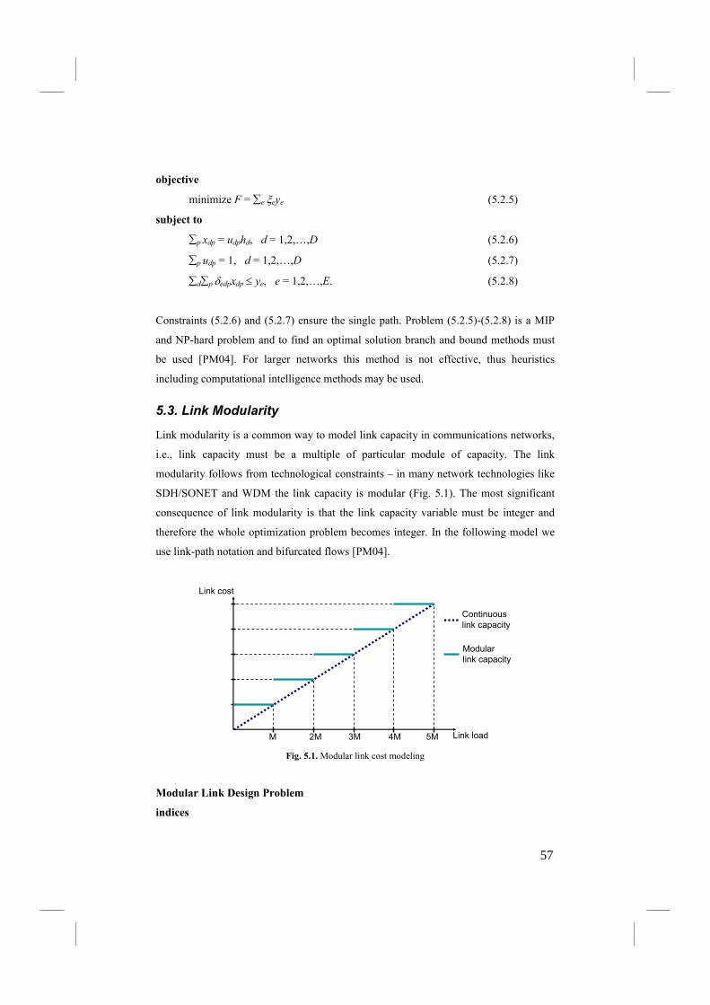
objective
minimize F = ∑e ξeye (5.2.5)
subject to
∑p xdp = udphd, d = 1,2,…,D (5.2.6)
∑p udp = 1, d = 1,2,…,D (5.2.7)
∑d∑p δedpxdp ≤ ye, e = 1,2,…,E. (5.2.8)
Constraints (5.2.6) and (5.2.7) ensure the single path. Problem (5.2.5)-(5.2.8) is a MIP
and NP-hard problem and to find an optimal solution branch and bound methods must
be used [PM04]. For larger networks this method is not effective, thus heuristics
including computational intelligence methods may be used.
5.3. Link Modularity
Link modularity is a common way to model link capacity in communications networks,
i.e., link capacity must be a multiple of particular module of capacity. The link
modularity follows from technological constraints – in many network technologies like
SDH/SONET and WDM the link capacity is modular (Fig. 5.1). The most significant
consequence of link modularity is that the link capacity variable must be integer and
therefore the whole optimization problem becomes integer. In the following model we
use link-path notation and bifurcated flows [PM04].
Link load
Link cost
M 2M 3M 4M 5M
Continuous
link capacity
Modular
link capacity
Fig. 5.1. Modular link cost modeling
Modular Link Design Problem
indices
57
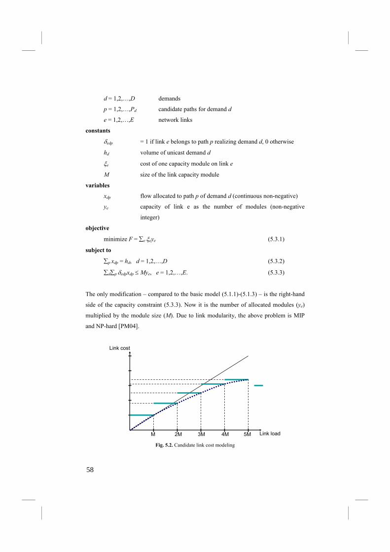
d = 1,2,…,D demands
p = 1,2,…,Pd candidate paths for demand d
e = 1,2,…,E network links
constants
δedp = 1 if link e belongs to path p realizing demand d, 0 otherwise
hd volume of unicast demand d
ξe cost of one capacity module on link e
M size of the link capacity module
variables
xdp flow allocated to path p of demand d (continuous non-negative)
ye capacity of link e as the number of modules (non-negative
integer)
objective
minimize F = ∑e ξeye (5.3.1)
subject to
∑p xdp = hd, d = 1,2,…,D (5.3.2)
∑d∑p δedpxdp ≤ Mye, e = 1,2,…,E. (5.3.3)
The only modification – compared to the basic model (5.1.1)-(5.1.3) – is the right-hand
side of the capacity constraint (5.3.3). Now it is the number of allocated modules (ye)
multiplied by the module size (M). Due to link modularity, the above problem is MIP
and NP-hard [PM04].
Link load
Link cost
M 2M 3M 4M 5M Fig. 5.2. Candidate link cost modeling
58

Another way to model link capacity is the candidate link approach – for each
link there is a set of possible link capacities and one of them is to be selected (Fig. 5.2).
This approach is included in regulations of ITU-T as well as many telecoms construct
their offer in similar way [GN89], [Kas89], [Kas01]. An important business issue is that
unit capacity cost decreases with the increase of candidate link capacity. Thus, the
cost/capacity function can be approximated by a concave function. For each link e there
is a set of candidate link proposals indexed k = 1,2,…,Ke and each candidate link is
described by the cost ξek and capacity cek. A binary variable yek is 1, if the type k is
selected for link e.
Candidate Link Design Problem
indices (additional)
k = 1,2,…,Ke candidate link types for link e
constants (additional)
ξek cost of candidate link type k on link e
cek capacity of candidate link type k on link e
variables
xdp flow allocated to path p of demand d (continuous non-negative)
yek = 1, if link type k is selected for link e; 0, otherwise
objective
minimize F = ∑e∑k ξekyek (5.3.4)
subject to
∑p xdp = hd, d = 1,2,…,D (5.3.5)
∑k yek = 1, e = 1,2,…,E (5.3.6)
∑d∑p δedpxdp ≤ ∑k cekyek, e = 1,2,…,E. (5.3.7)
The objective function is the cost of selected candidate links. Constraint (5.3.6) assures
that for each link exactly one candidate link is selected. Notice that ∑k cekyek denotes the
capacity of e capacity, therefore this formula is used in right-hand side of (5.3.7). The
above problem is MIP and NP-complete.
59

5.4. Convex Problems
In this section we will focus on network design problem with a convex objective
function presented in [GN89]. The problem uses non-bifurcated flows, link-path
formulation and candidate link modeling. The objective is to minimize the cost
including both capacity and delay components. Moreover, we will show how to apply
Lagrangean relaxation and subgradient optimization techniques to this problem.
Convex Design Problem
indices (additional)
d = 1,2,…,D demands
p = 1,2,…,Pd candidate paths for demand d
e = 1,2,…,E network links
k = 1,2,…,Ke candidate link types for link e
constants
δedp = 1, if link e belongs to path p realizing demand d; 0, otherwise
hd volume of unicast demand d
ξe cost of one capacity module on link e
ξek cost of candidate link type k on link e
cek capacity of candidate link type k on link e
variables
xdp 1, if path p is used to realize demand d; 0, otherwise
yek = 1, if link type k is selected for link e; 0, otherwise
fe flow on link e (non-negative, continuous)
objective
minimize F = ∑e fe / (∑k cekyek – fe) + ∑e ∑k ξekyek (5.4.1)
subject to
∑d∑p δedpxdphd = fe, e = 1,2,…,E (5.4.2)
∑p xdp = 1, d = 1,2,…,D (5.4.3)
∑k yek = 1, e = 1,2,…,E (5.4.4)
fe ≤ ∑k cekyek, e = 1,2,…,E. (5.4.5)
60
Since the objective function is increasing in fe, the problem can be reformulated as:
Modified Convex Design Problem
objective
minimize F = ∑e fe / (∑k cekyek – fe) + ∑e ∑k ξekyek (5.4.6)
subject to
∑d∑p δedpxdphd ≤ fe, e = 1,2,…,E (5.4.7)
∑p xdp = 1, d = 1,2,…,D (5.4.8)
∑k yek = 1, e = 1,2,…,E (5.4.9)
0 ≤ fe ≤ ∑k cekyek, e = 1,2,…,E. (5.4.10)
Let λλλλ = [λ1, λ2,…,λE] be a vector of Lagrangian multipliers. Constraint (5.4.7) is relaxed
and the corresponding Lagrangian function is as follows:
L(λλλλ) = (∑e fe/(∑k cekyek – fe) + ∑e∑k ξekyek) + ∑eλe (∑d∑p δedphdxdp – fe). (5.4.11)
After simple calcualation we obtain:
L(λλλλ) = ∑e fe/(∑k cekyek – fe) + ∑e∑k ξekyek – ∑e λefe + ∑e∑d∑p δedpλexdudp. (5.4.12)
Recall, that the main idea of Lagrangean relaxation is to formulate the dual
problem by relaxing some constraints of the primal problem and next solving the dual
by a subgradient algorithm. The solutions to the Lagrangean problem yielded at each of
the iterations of the subgradient algorithm can be used as an initial solution for
generating feasible solutions to the considered network design problem. Since the value
of the optimal solution is between the lower bound and the value of the best feasible
solution available found by any heuristic algorithm, the quality of the heuristic solution
can thus be evaluated [GN89].
As variables fe and xdp are not linked (there are no constraints that includes both
kinds of variables), we receive D + E subproblems, that can be solved independently.
The first subproblem includes the part of Lagrangean function (5.4.12) related variables
xdp and constraints including variables xdp. There is one subproblem for each link
d = 1,2,…,D.
Subproblem 1
objective
minimize Ld(λλλλ) = ∑e∑p δedpλehdudp (5.4.13)
61
constraints
∑p xdp = 1. (5.4.14)
To solve the above subproblem, we must find the shortest path p = 1,2,…,Pd under the
metric λe , so it is quite easy to find the solution.
The second subproblem includes the part of Lagrangean function related
variables yek and fe as well as constraints including variables yek and fe. The subproblem
is formulated for each link e = 1,2,…,E.
Subproblem 2
objective
minimize Le(λλλλ) = fe/(∑k cekyek – fe) + ∑k ξekyek – λefe (5.4.15)
constraints
∑k yek = 1, (5.4.16)
0 ≤ fe ≤ ∑kcek yek. (5.4.17)
Since the number of candidate link proposals Ke is relatively small for each link, we can
solve the Subproblem 2 for each k = 1,2,…,Ke separately.
Decoupled Subproblem 2
objective
minimize Le(λ,k) = fe/(cek – fe) + ξek – λe fe (5.4.18)
constraints
0 ≤ fe ≤ cek. (5.4.19)
The solution of the Decoupled Subproblem 2 (5.4.18)-(5.4.19) is:
>−
=otherwise0
/1when)/()( ekeeekek
e
ccckf
λλ. (5.4.19)
Futher details on the Subgradient procedure can be found in [GN89].
5.5. Example
In the example we consider various variants of network design problems presented
above in the context of the network (Fig. 4.3) considered in Section 4.5. To recall, the
62
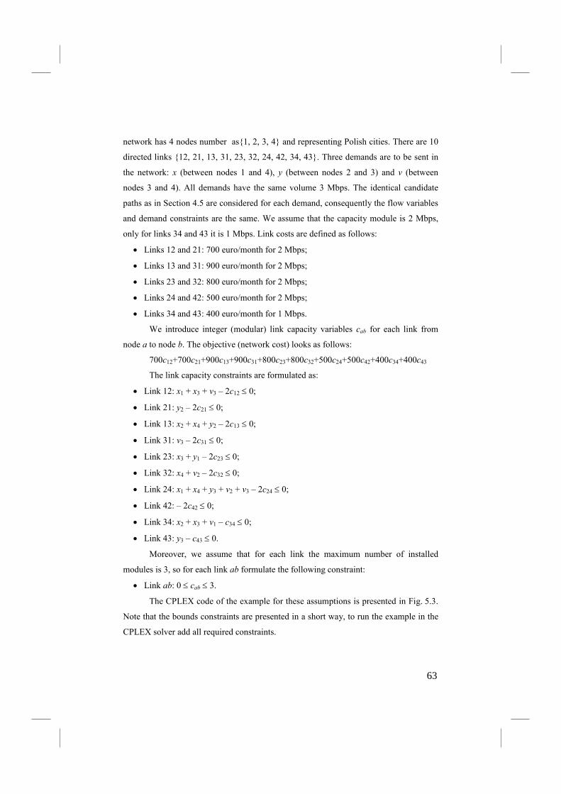
network has 4 nodes number as{1, 2, 3, 4} and representing Polish cities. There are 10
directed links {12, 21, 13, 31, 23, 32, 24, 42, 34, 43}. Three demands are to be sent in
the network: x (between nodes 1 and 4), y (between nodes 2 and 3) and v (between
nodes 3 and 4). All demands have the same volume 3 Mbps. The identical candidate
paths as in Section 4.5 are considered for each demand, consequently the flow variables
and demand constraints are the same. We assume that the capacity module is 2 Mbps,
only for links 34 and 43 it is 1 Mbps. Link costs are defined as follows:
• Links 12 and 21: 700 euro/month for 2 Mbps;
• Links 13 and 31: 900 euro/month for 2 Mbps;
• Links 23 and 32: 800 euro/month for 2 Mbps;
• Links 24 and 42: 500 euro/month for 2 Mbps;
• Links 34 and 43: 400 euro/month for 1 Mbps.
We introduce integer (modular) link capacity variables cab for each link from
node a to node b. The objective (network cost) looks as follows:
700c12+700c21+900c13+900c31+800c23+800c32+500c24+500c42+400c34+400c43
The link capacity constraints are formulated as:
• Link 12: x1 + x3 + v3 – 2c12 ≤ 0;
• Link 21: y2 – 2c21 ≤ 0;
• Link 13: x2 + x4 + y2 – 2c13 ≤ 0;
• Link 31: v3 – 2c31 ≤ 0;
• Link 23: x3 + y1 – 2c23 ≤ 0;
• Link 32: x4 + v2 – 2c32 ≤ 0;
• Link 24: x1 + x4 + y3 + v2 + v3 – 2c24 ≤ 0;
• Link 42: – 2c42 ≤ 0;
• Link 34: x2 + x3 + v1 – c34 ≤ 0;
• Link 43: y3 – c43 ≤ 0.
Moreover, we assume that for each link the maximum number of installed
modules is 3, so for each link ab formulate the following constraint:
• Link ab: 0 ≤ cab ≤ 3.
The CPLEX code of the example for these assumptions is presented in Fig. 5.3.
Note that the bounds constraints are presented in a short way, to run the example in the
CPLEX solver add all required constraints.
63
The obtained solution of link capacities is as follows: c12 = 2; c21 = 0; c13 = 0;
c31 = 0; c23 = 1; c32 = 0; c24 = 2; c42 = 0; c34 = 3; c43 = 1. This yields the total network
cost equal to 4800 euro/month.
Minimize obj: 700c12 + 700c21 + 900c13 + 900c31 + 800c23 + 800c32 + 500c24
+ 500c42 + 400c34 + 400c43 Subject To x: x1 + x2 + x3 +x4 = 3
y: y1 + y2 + y3 = 3 v: v1 + v2 + v3 = 3
c12: x1 + x3 + v3 - 2c12 <= 0 c21: y2 - 2c21 <= 0 c13: x2 + x4 + y2 - 2c13 <= 0
c31: v3 - 2c31 <= 0 c23: x3 + y1 - 2c23 <= 0
c32: x4 + v2 - 2c32 <= 0 c24: x1 + x4 + y3 + v2 + v3 - 2c24 <= 0 c42: -2c42 <= 0
c34: x2 + x3 + v1 - c34 <= 0 c43: y3 - c43 <= 0
Bounds 0 <= x1 <= 3 ...
0 <= v3 <= 3 0 <= c12 <= 3
... 0 <= c43 <= 3 Integers
c12 c21 c13 c31 c23 c32 c24 c42 c34 c43 End
Fig. 5.3. CPLEX code of the example for link-path notation
Now we report other examples. First, we set the maximum number of installed
capacity modules to 4, i.e. the following constraint is added to the model:
• Link ab: 0 ≤ cab ≤ 4.
In this case the solution is the same as in previous case (4800 euro/month).
However, when we set the maximum number of installed capacity modules to 2, we
obtain the network cost equal to 5600 euro/month. This follows from the fact that
limited number of capacity modules enforces to route the demands on more expensive
paths that include links with higher unit costs. Note that if we let the capacity variables
to be continuous, we obtain for the previous case (limit of 2 modules) the network cost
of 4450 euro/month.
In further experiments we assume non-bifurcated flows, i.e., demand flow
variables are binary. The link capacity can be continuous, i.e., the link modularity is not
considered. If the maximum number of capacity modules is set to 2, there is no any
64

feasible solution. In the case when the maximum number of capacity modules is 3, the
obtained cost is 4200 euro/month. If we assume for this case integer capacity variables
(modular links) we obtain cost 5200 euro/month. Recall that in the same case, but for
bifurcated flows the cost was 4800 euro/month. So the profit of using bifurcated flows
is 400 euro/month.
5.6. Exercises
5.1. Can we use the Shortest-Path Allocation Rule for the Incremental Design Problem
(5.1.12)-(5.1.24)?
5.2. Can we use the Shortest-Path Allocation Rule for the Path Diversity Design
Problem (5.2.1)-(5.2.4)?
5.3. Rewrite the path diversity (5.2.1)-(5.2.4) to enforce that each demand uses exactly
two paths.
5.4. Can we use the Shortest-Path Allocation Rule for the Modular Link Design
Problem (5.3.1)-(5.3.3)?
5.5. Write the Modular Link Design Problem assuming that there are several possible
sizes of the capacity module.
5.6. Propose a method to calculate a lower bound for the Modular Link Design Problem.
5.7. Construct a computational intelligence algorithm for a selected network design
problem.
5.8. Write and solve the Lagrangean relaxation for the Convex Design Problem with
bifurcated flows.
5.9. Propose a method to calculate a lower bound for the Convex Design Problem.
5.10. Write the CPLEX code for all examples considered in Section 5.5.
65
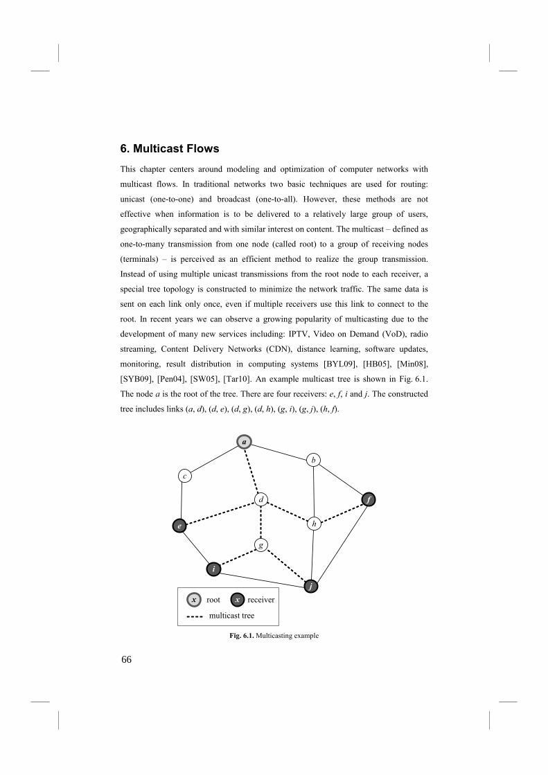
6. Multicast Flows
This chapter centers around modeling and optimization of computer networks with
multicast flows. In traditional networks two basic techniques are used for routing:
unicast (one-to-one) and broadcast (one-to-all). However, these methods are not
effective when information is to be delivered to a relatively large group of users,
geographically separated and with similar interest on content. The multicast – defined as
one-to-many transmission from one node (called root) to a group of receiving nodes
(terminals) – is perceived as an efficient method to realize the group transmission.
Instead of using multiple unicast transmissions from the root node to each receiver, a
special tree topology is constructed to minimize the network traffic. The same data is
sent on each link only once, even if multiple receivers use this link to connect to the
root. In recent years we can observe a growing popularity of multicasting due to the
development of many new services including: IPTV, Video on Demand (VoD), radio
streaming, Content Delivery Networks (CDN), distance learning, software updates,
monitoring, result distribution in computing systems [BYL09], [HB05], [Min08],
[SYB09], [Pen04], [SW05], [Tar10]. An example multicast tree is shown in Fig. 6.1.
The node a is the root of the tree. There are four receivers: e, f, i and j. The constructed
tree includes links (a, d), (d, e), (d, g), (d, h), (g, i), (g, j), (h, f).
x root
d
a
c
e
b
h
g
f
i
j
x receiver
multicast tree
Fig. 6.1. Multicasting example
66
Multicast modeling can use two classical network problems:
• Steiner tree problem. Given a set V of points (network nodes), interconnect them
by a subgraph of shortest length (sum of the lengths of all edges).
• Minimum Spanning Tree (MST) problem is a subgraph of the orginal graph
(network), which is a tree (no loops) and connects all the vertices together.
The difference between both problems is that in the Steiner tree problem extra
intermediate vertices (Steiner vertices) and edges may be added to the graph in order to
reduce the length of the spanning tree.
Multicasting can be divided into two categories:
• Traditional IP multicast – is a method to send packets to a group of interested
receivers in a single transmission. The multicasting is applied in layer 3 and IP
routers are responsible for creating the delivery tree. End hosts (receivers) are
leafs of the tree. IP multicast uses the following protocols:
o Protocol-Independent Multicast (PIM) – is a family of IP multicast
protocols that provide one-to-many and many-to-many distribution of
data over an IP network. PIM is protocol-independent, since it does not
include its own topology discovery mechanism, but instead uses routing
information supplied by other traditional routing protocols (e.g., BGP).
o Internet Group Management Protocol (IGMP) – is a protocol used to
manage the membership of IP multicast groups. IGMP is used by hosts
and adjacent multicast routers to establish multicast group memberships.
• Overlay multicast (Peer-to-Peer multicast, application-layer multicast) – is
realized in the application layer. End hosts (receivers) can also upload the
multicast stream to other nodes (peers).
For more information on various aspects of multicasting refer to [Min08].
6.1. Modeling of Multicast Flows
Multicast flows can be modeled in several ways. In this section we present four
proposals of multicast formulations:
• Canonical Formulation.
• Flow Formulation.
• Level Formulation.
67
• Candidate Tree Formulation.
All formulations will be presented in the context of the flow allocation problem, i.e., an
existing network with fixed link capacity is considered. However, the formulation can
be used in other types of network optimization problems, e.g., capacity and flow
optimization or resource location problems.
The first presented formulation is called canonical [KM98]. The multicast
transmission is modeled using the Steiner tree problem. For each network link (edge) e,
there is a variable xe indicating whether e is in the Steiner tree (xe = 1) or not (xe = 0).
The formulation uses cuts of the original network graph G = (V, E), where V denotes set
of nodes and E set of links. Set T denotes set of terminals (receivers of the
multicasting). We assume that δ(W) defines a graph cut induced by W⊆V, i.e., δ(W)
includes a set of edges with the source node in set W and the destination node in its
complement set (V \ W).
Canonical Multicast Formulation
sets
V network nodes
E links (directed edges)
T terminals (receivers)
indices
e links (edges)
constants
δ(W) cut induced by W⊆V, including edges with the source node in W
and the destination node in its complement (V \ W)
s root node of multicast tree
hd volume (bandwidth requirement) of multicasting
ce capacity of link e
variables
xe = 1, if multicast tree uses link e; 0, otherwise (binary)
subject to
x(δ(W)) ≥ 1, for all W⊂V, s∈W, (V \ W)∩T ≠ 0 (6.1.1)
x(W) = ∑e∈W xe, (6.1.2)
xeh ≤ ce, e ∈ E. (6.1.3)
68

The most important element of the model is defined in (6.1.1) and (6.1.2), i.e., for every
cut x(δ(W)) in the network between a subset of nodes W including the root node s and
the complement set of nodes (V \ W) including at least one terminal node (receiver of
the multicasting) must be at least one link (defined by x(δ(W))). This formulation
assures that there is a path from the root node to every terminal node and consequently,
each receiver is connected to the multicasting. Condition (6.1.3) is the capacity
constraint that guarantees that the link flow (given by xeh) cannot exceed the link
capacity. The main drawback of the canonical formulation is that the number of
possible cuts grows exponentially with the network size (number of nodes). Note that
the above problem does not include an objective function. However, various criterion
functions defined on the multicast flows can be used, for more details see following
subsections. Further information on the canonical formulation of multicasting refer to
[KM98].
To illustrate the canonical example we analyze the network presented in Fig. 6.1.
For instance, set W = {a, b, c} induces a correct cut δ(W) = {(a, d), (b, f), (b, h), (c, e)}.
Since link (a, d) is in the multicast tree, the condition (6.1.1) is satisfied, i.e.,
x(δ(W) ) = 1. Notice that if W = {a, b, c, d}, then x(δ(W) ) = 3. That is why the (6.1.1)
condition is greater or equal 1. On the contrary, W = {c, e, i} is not feasible, since it
does not include the root node a. Another example of incorrect set is
W = {a, c, e, f, i, j}, as the complement set of nodes (V \ W) does not contain any
receiving nodes.
The next formulation – referred to as flow formulation – is based on the
multicommodity flow formulation developed for unicast flows [DGR06], [LLJ05],
[OPR06], [WL05], [WL07]. It is easy to notice that the node-link formulation
developed for unicast flows can be modified for the use in the context of multicast
flows. The network graph is defined by links indexed e = 1,2,…,E. The multicast
demand is defined by a source node s and a set of terminal nodes (receivers) indexed by
k = 1,2,…,K. The general idea underlying this approach is to define for every terminal
node a unicast path connecting the root node and the terminal node. For this purpose we
use a binary variable xek, which is 1, if multicast flow from the root to receiver k uses
link e and 0 otherwise. However, this can lead to the fact that on some network links the
same data issued by the root node is sent several times and consumes the network
69
bandwidth in an excessive way. Therefore, an additional binary variable xe associated
with each link e is incorporated in the model to assure that the multicast flow goes
through a link at most once. Variable xe equals 1, if multicast tree uses link e; 0,
otherwise.
Flow Multicast Formulation
indices
v = 1,2,…,V network nodes
e = 1,2,…,E links
k = 1,2,…,K terminals (receivers)
constants
aev = 1, if link e originates at node v; 0, otherwise
bev = 1, if link e terminates in node v; 0, otherwise
s root node of multicast tree
h volume (bandwidth requirement) of multicast
ce capacity of link e
variables
xek = 1, if multicast flow to receiver k uses link e; 0, otherwise
xe = 1, if multicast tree uses link e; 0, otherwise (binary)
subject to
∑e aevxek – ∑e bevxek = 1, v = s v = 1,2,…,V k = 1,2,…,K (6.1.4)
∑e aevxek – ∑e bevxek = –1, v = k v = 1,2,…,V k = 1,2,…,K (6.1.5)
∑e aevxek – ∑e bevxek = 0, v ≠ s,k v = 1,2,…,V k = 1,2,…,K (6.1.6)
xek ≤ xe, e = 1,2,…,E k = 1,2,…,K (6.1.7)
xeh ≤ ce, e = 1,2,…,E. (6.1.8)
Constraints (6.1.4)-(6.1.6) define unicast paths connecting the root node s and each
terminal using the node-link formulation of multicommodity flows. Recall that the left-
hand side of constraints (6.1.4)-(6.1.6) is the total number of outgoing links minus the
total number of incoming links of the unicast path defined for each network node v and
each receiver k. Thus, if the considered node v is the root node s (6.1.4), the right-hand
side must be 1. If the node v is a terminal node, it must be –1. Ale remaining nodes are
transit nodes, and the flow balance must be 0. Constraint (6.1.7) is in the model to
70

assure that each link is used in the multicast at most one time. The variable xe is
switched on, only if the particular link e is in the unicast path to at least one receiver k.
Finally, (6.1.8) is a capacity constraint.
To exemplify the flow formulation we use the network in Fig. 6.1. First, we
analyze the flow conservation law (6.1.4)-(6.1.6). Let’s focus on a path between nodes a
and e including links (a, d) and (d, e). Node a has one leaving multicast link (a, d),
therefore constraint (6.1.4) is satisfied. The receiving node e contains one incoming
multicast link (d, e), so constraint (6.1.5) holds. All other remaining nodes – according
to condition (6.1.6) – has the same number of outgoing and incoming links. Next, notice
that link (a, d) carries 4 unicast paths to receiving nodes e, f, i and j. However, the
definition of binary variable xe (6.1.7) guarantees that the (a, d) link sends only one
copy of the multicast flow and in the capacity constraint (6.1.8) the link (a, d) flow is
equal to the volume of multicasting given by h. A similar situation is in the case of link
(d, g) that carries two unicast paths to receivers i and j.
The next formulation called level assumes that the multicast tree is divided into
subsequent levels [Wal09a]. We assume that the root of the tree is located on level 1.
All children of the root (nodes that have a direct link from the root) are located on level
2. Summarizing, we assume that if a father node of v is on level l, then the v is located
on level (l + 1). Comparing to the flow formulation, we denote network links in a
different way, i.e., a pair of nodes (w,v) defines a network link from node w to node v.
Additional binary constant e(w,v) denotes, if there is a direct link (w,v) in the network
graph. To model the multicast tree we use a binary variable xwvl that is 1 only, if the link
(w,v) is used in multicast tree and w is located on level l of the tree. As in the flow
formulation, we use a variable xwv to denote if a link (w,v) is in the multicast tree. Note
that this formulation is also referred to as layered graphs [GLU09].
The level formulation is used in the hop-constrained multicasting, i.e., there is an
upper limit L on the number of hops between the root node and any other node
[DGR06]. The motivation of this additional constraint to limit hop count is to improve
the QoS (Quality of Service) parameters of the P2P multicasting including network
reliability and transmission delay.
Level Multicast Formulation
indices
v,w,b = 1,2,…,V network nodes
71
k = 1,2,…,K terminals (receivers)
l = 1,2,…,L levels
constants
s root node of multicast tree
h volume (bandwidth requirement) of multicast
e(w,v) =1, if there is a direct link (w,v) in graph; 0, otherwise
cwv capacity of link (w,v)
variables
xwvl = 1, if the link (w,v) is used in multicast tree and w is located on
level l of the tree; 0, otherwise (binary)
xwv = 1, if multicast tree uses link e; (w,v), otherwise (binary)
subject to
∑w:e(w,v)=1 ∑l xwvl = 0, v = s v = 1,2,…,V (6.1.9)
∑w:e(w,k)=1 ∑l xwkl = 1, k = 1,2,…,K (6.1.10)
∑v:e(w,v)=1 xwv1 = 0, w ≠ s w = 1,2,…,V (6.1.11)
xwv(l+1) ≤ ∑b xbwl, e(w,v) = 1 w = 1,2,…,V v = 1,2,…,V
l = 1,2,…,L – 1 (6.1.12)
∑l xwvl ≤ xwv, e(w,v) = 1 w = 1,2,…,V v = 1,2,…,V (6.1.13)
xwv ≤ ∑l xwvl, e(w,v) = 1 w = 1,2,…,V v = 1,2,…,V (6.1.14)
xwvh ≤ cwv, e(w,v) = 1 w = 1,2,…,V v = 1,2,…,V. (6.1.15)
Condition (6.1.9) assures that the root node s cannot download and multicast flow, i.e.,
the total flow on all links (w,v) (defined as e(w,v) = 1) entering node v = s must be zero.
Constraint (6.1.10) guarantees that each receiving node k = 1,2,…,K must be connected
to the multicast tree. To meet the requirement that a node w cannot be the parent of the
first level link, if w is not the root node (w ≠ s) we add constraint (6.1.11). Condition
(6.1.12) is in the model to assure that each node w cannot upload multicast flow to any
other node v on level (l + 1), if w is not located on level l of the multicast tree. Notice
that the right-hand side of (6.1.12) denotes the number of multicast links entering node
w on level l. If there is none such link, the left-hand side of (6.1.12) must be 0.
Constraints (6.1.13) and (6.1.14) are used to bind variables xwvl and xwv. (6.1.13)
guarantees that if for any level l there is link between nodes w and v in the multicast tree
(∑l xwv = 1), then xwv must be 1. (6.1.14) assures that if there is no link between nodes w
72
and v on any level l (∑l xwv = 1), consequently xwv is 1. Condition (6.1.15) is the capacity
constraint.
Now we analyze the level formulation in the context of the example network
shown in Fig. 6.1. The root node a is located on level 1. Nodes b, d and f are on level 2.
The next level 3 includes nodes e, g and h. Finally, remaining nodes f, i and j are on
level 4. The multicast tree shown in Fig. 6.1 is defined by the following variables xwvl
equal to 1: xad1, xde2, xdg2, xdh2, xgi3, xgj3, xhf3. All remaining xwvl variables are equal to 0.
It is easy to check that these variables satisfy all constraints of the level formulation.
The main advantage of the level formulation comparing to the flow formulation,
is lower complexity expressed by the number of variables. Recall that the level
formulation uses (EL + E) variables while the flow formulation includes (EK + E)
variables (E is the number of links, K number of receivers, L number of levels). Usually
the level number L is much lower than the number of receivers.
The last formulation called candidate tree takes inspiration from the link-path
modeling of unicast flows. We assume that there is a set candidate tree topologies
connecting the same root node and all terminals (receivers) indexed p = 1,2,…,P.
Continuous decision variable xp denotes the amount of multicast flow allocated to tree
topology p.
Candidate Tree Formulation
indices
e = 1,2,…,E links
p = 1,2,…,P candidate trees
constants
δep = 1, if link e belongs to tree p; 0, otherwise
h volume (bandwidth requirement) of multicast
variables
xp flow allocated to tree p (continuous non-negative)
constraints
∑p xp = h, (6.1.16)
∑p δepxph ≤ ce, e = 1,2,…,E. (6.1.17)
73

The model is very simple and includes only two conditions. The former constraint
(6.1.16) assures that the whole volume of multicasting should be sent in the network.
The latter one (6.1.1.7) is the capacity constraint. Note that in the above model we let
the multicast flow to be split to many trees, however a nonsplitable version of the
formulation can be easily written. The candidate tree formulation has the same
shortcomings as analogous unicast link-path modeling. First, if the set of candidate trees
is not selected in a proper way, the obtained solution has no guarantee to be optimal in a
global way. Second, since the number of all possible trees can be enormous, some
methods to limit the set of candidate trees are required.
6.2. Cost Problem
The first problem we will formulate has the objective to minimize the routing cost of
multicasting. For each link between nodes w and v a constant ζwv denotes the cost of
using this link in the multicasting. The criterion function is defined as the total cost of
all links included in the multicast tree scaled by the amount of flow carried on the link.
We assume that the multicast flow can be split to multiple trees indexed t = 1,2,…,T,
however the number of used trees is upper bounded. Moreover, the volume of
multicasting on each tree denoted by ht is given. In the model the level formulation is
applied.
Multicast Cost Problem
indices
v,w,b = 1,2,…,V network nodes
k = 1,2,…,K terminals (receivers)
l = 1,2,…,L levels
t = 1,2,…,T trees
constants
s root node of multicast tree
ht volume (bandwidth requirement) of multicast tree t
e(w,v) =1, if there is a direct link (w,v) in graph; 0, otherwise
cwv capacity of link (w,v)
ζwv routing cost of link (w,v)
74

variables
xwvtl = 1, if the link (w,v) is used in multicast tree t and w is located on
level l of the tree; 0, otherwise (binary)
xwvt = 1, if multicast tree t uses link (w,v), 0, otherwise (binary)
objective
minimize F = ∑w ∑v ∑ xwvthtζwv (6.2.1)
subject to
∑w:e(w,v)=1 ∑l xwvtl = 0, v = s v = 1,2,…,V t = 1,2,…,T (6.2.2)
∑w:e(w,k)=1 ∑l xwktl = 1, k = 1,2,…,K t = 1,2,…,T (6.2.3)
∑v:e(w,v)=1 xwvt1 = 0, w ≠ s w = 1,2,…,V t = 1,2,…,T (6.2.4)
xwvt(l+1) ≤ ∑b xbwtl, e(w,v) = 1 w = 1,2,…,V v = 1,2,…,V
l = 1,2,…,L – 1 t = 1,2,…,T (6.2.5)
∑l xwvtl ≤ xwvt, e(w,v) = 1 w = 1,2,…,V v = 1,2,…,V
t = 1,2,…,T (6.2.6)
xwvt ≤ ∑l xwvtl, e(w,v) = 1 w = 1,2,…,V v = 1,2,…,V
t = 1,2,…,T (6.2.7)
∑t xwvtht ≤ cwv, e(w,v) = 1 w = 1,2,…,V v = 1,2,…,V. (6.2.8)
The objective function (6.2.1) denotes the multicast routing cost. Constraints (6.2.2)-
(6.2.8) are equivalent to the level formulation (6.1.9)-(6.1.15). The only modification
follows from the fact that multiple trees can be used. Therefore, constraints (6.2.2)-
(6.2.7) are repeated for each tree. In the capacity constraint, the left-hand side includes
the sum over all trees. Note that the above problem is linear, integer (binary) and NP-
complete (equivalent to the Steiner tree problem).
6.3. Network Design Problem
In this section we show a multicast version of the network design problem. Both link
capacity and multicast flows are to be optimized in order to minimize the network cost
defined as cost of selected links. We assume that several multicast demands
d = 1,2,…,D are to be served in the network. Each demand d is defined by the root node
sd, set of receivers indexed k = 1,2,…,Kd and volume hd. We use the flow formulation
and modular link modeling.
75

Multicast �etwork Design Problem
indices
d = 1,2,…,D multicast demands
v = 1,2,…,V network nodes
e = 1,2,…,E links
k = 1,2,…,Kd terminals (receivers) of demand d
constants
aev = 1, if link e originates at node v; 0, otherwise
bev = 1, if link e terminates in node v; 0, otherwise
sd root node of multicast demand d
hd volume (bandwidth requirement) of multicast demand d
ξe cost of one capacity module on link e
M size of the link capacity module
variables
xedk = 1, if multicast flow of multicast demand d to receiver k uses link
e; 0, otherwise (binary)
xed = 1, if multicast demand d uses link e; 0, otherwise (binary)
ye capacity of link e as the number of modules (non-negative
integer)
objective
minimize F = ∑e ξeye (6.3.1)
subject to
∑e aevxedk – ∑e bevxedk = 1, v = sd v = 1,2,…,V d = 1,2,…,D
k = 1,2,…,Kd (6.3.2)
∑e aevxedk – ∑e bevxedk = –1, v = k v = 1,2,…,V d = 1,2,…,D
k = 1,2,…,Kd (6.3.3)
∑e aevxedk – ∑e bevxedk = 0, v ≠ sd,k v = 1,2,…,V d = 1,2,…,D
k = 1,2,…,Kd (6.3.4)
xedk ≤ xed, e = 1,2,…,E d = 1,2,…,D k = 1,2,…,Kd (6.3.5)
∑d xedh ≤ Mye, e = 1,2,…,E. (6.3.6)
The objective is the cost of link capacity. Constraints (6.3.2)-(6.3.5) are equivalent to
the flow formulation (6.1.4)-(6.1.7), however additional demand index d is included.
76
The capacity constraint is modified on both sides. The left-hand side defines the link
flow as a sum over all multicast demands that use the particular link. The right-hand
side of the capacity constraint is calculated according to the selected number of modules
to be installed on this link. The problem belongs to the class of linear integer programs.
Moreover, since it is NP-complete (equivalent to the Steiner tree problem).
6.4. Maximum Delay Problem
The next problem has the objective to minimize the maximum delivery delay taking into
account all receivers of the multicasting. We apply the flow formulation, since it is
impossible to define the maximum delay function in the level formulation. We assume
that each link e = 1,2,…,E is associated with a communication delay ζe given in
milliseconds. For each receiving node k = 1,2,…,K we can calculate the arrival latency
of k taking into account the whole path from the root of tree t to k using formula
∑e xekζe. Recall that variable xek is 1, if multicast flow to receiver k uses link e and 0
otherwise. The overall goal is to minimize the maximum value of this delay over all
receiving nodes.
Multicast Maximum Delay Problem
indices
v = 1,2,…,V network nodes
e = 1,2,…,E links
k = 1,2,…,K terminals (receivers)
constants
aev = 1, if link e originates at node v; 0, otherwise
bev = 1, if link e terminates in node v; 0, otherwise
s root node of multicast tree
h volume (bandwidth requirement) of multicast
ce capacity of link e
ζe delay of link e
variables
xek = 1, if multicast flow to receiver k uses link e; 0, otherwise
xe = 1, if multicast tree uses link e; 0, otherwise (binary)
x maximum delay (non-negative continuous)
objective
77
minimize x (6.4.1)
subject to
∑e aevxek – ∑e bevxek = 1, v = s v = 1,2,…,V k = 1,2,…,K (6.4.2)
∑e aevxek – ∑e bevxek = –1, v = k v = 1,2,…,V k = 1,2,…,K (6.4.3)
∑e aevxek – ∑e bevxek = 0, v ≠ s,k v = 1,2,…,V k = 1,2,…,K (6.4.4)
xek ≤ xe, e = 1,2,…,E k = 1,2,…,K (6.4.5)
xeh ≤ ce, e = 1,2,…,E (6.4.6)
∑e ζexek ≤ x, k = 1,2,…,K. (6.4.7)
The novelty of the above model comparing against the flow formulation presented in
Section 6.1 is a new variable x that denotes the maximum delay. A new condition
(6.4.7) is formulated to define x as the upper bound of delays over all receivers
k = 1,2,…,K. As previous problems, the maximum delay problem is linear, integer
(binary) and NP-complete (equivalent to the Steiner tree problem).
6.5. Throughput Problem
The next objective function we consider is the system throughput, i.e., we want to
maximize the aggregate receiving rate at each participating node [WL07]. We assume
as in Section 6.2 that the multicast flow is transmitted using several trees t = 1,2,…,T.
For each tree t we have an additional variable qt denoting the volume (throughput) of
the tree. The objective is to maximize the overall throughput defined by ∑t qt. To
formulate the problem we use a modified version of the level formulation. However,
note also that the flow formulation can be applied in this case, but some extra flow
variables will be required what additionally complicates the model. The main
modification of the level formulation presented in Section 6.1 is that the xwvtl variable
denotes the streaming rate on an link (w,v) in multicast tree t and w is located on level l
of tree t. Consequently, the variable xwvtl is in this case continuous.
Multicast Throughput Problem
indices
v,w,b = 1,2,…,V network nodes
k = 1,2,…,K terminals (receivers)
l = 1,2,…,L levels
78
t = 1,2,…,T trees
constants
s root node of multicast tree
e(w,v) =1, if there is a direct link (w,v) in graph; 0, otherwise
cwv capacity of link (w,v)
M large number
variables
xwvtl streaming rate on an overlay link (w,v) (no other nodes in
between) in multicast tree t and w is located on level l of tree t;
(continuous, non-negative)
xwvt = 1, if multicast tree t uses link (w,v); 0, otherwise (binary)
qt throughput (bandwidth requirement) of tree t (continuous, non-
negative)
objective
maximize F = ∑t qt (6.5.1)
subject to
∑w:e(w,v)=1 ∑l xwvtl = 0, v = s v = 1,2,…,V t = 1,2,…,T (6.5.2)
∑w:e(w,k)=1 ∑l xwktl = qt, k = 1,2,…,K t = 1,2,…,T (6.5.3)
∑v:e(w,v)=1 xwvt1 = 0, w ≠ s w = 1,2,…,V t = 1,2,…,T (6.5.4)
xwvt(l+1) ≤ ∑b xbwtl, e(w,v) = 1 w = 1,2,…,V v = 1,2,…,V
l = 1,2,…,L – 1 t = 1,2,…,T (6.5.5)
∑l xwvtl ≤ Mxwvt, e(w,v) = 1 w = 1,2,…,V v = 1,2,…,V
t = 1,2,…,T (6.5.6)
xwvt ≤ ∑l xwvtl, e(w,v) = 1 w = 1,2,…,V v = 1,2,…,V
t = 1,2,…,T (6.5.7)
∑t∑l xwvtl ≤ cwv, e(w,v) = 1 w = 1,2,…,V v = 1,2,…,V. (6.5.8)
The objective (6.5.1) is the system throughput. The modification of the model can be
observed in (6.5.3). Note that the right-hand side of constraint (6.5.3) is the throughput
of tree t, i.e., the amount of flow that must receive each receiver. The next change is in
(6.5.6) – the large number M is used to bind variables xwvtl and xwvt. Finally, in the
capacity constraint (6.5.8) we calculate the link flow (right-hand side) as the sum over
79
all trees t and levels l. The above problem is linear, mixed integer (binary) and NP-
complete (equivalent to the Steiner tree problem).
6.6. Multicast Packing Problem
In this section we address the problem of capacity planning in a network with multicast
flows. The idea is to minimize the maximum network congestion defined as the
maximum link load. As in Section 6.3, there are several multicast demands d = 1,2,…,D
in the network, described by the root node sd, set of receivers indexed k = 1,2,…,Kd and
volume hd. The considered problem – called multicast packing problem – has attracted
considerable attention from researchers in the area of multicast [OPR06]. In the
formulation we apply the flow modeling of multicast flows.
Multicast Packing Problem
indices
d = 1,2,…,D multicast demands
v = 1,2,…,V network nodes
e = 1,2,…,E links
k = 1,2,…,Kd terminals (receivers) of demand d
constants
aev = 1, if link e originates at node v; 0, otherwise
bev = 1, if link e terminates in node v; 0, otherwise
sd root node of multicast demand d
hd volume (bandwidth requirement) of multicast demand d
M size of the link capacity module
variables
xedk = 1, if multicast flow of multicast demand d to receiver k uses link
e; 0, otherwise (binary)
xed = 1, if multicast demand d uses link e; 0, otherwise (binary)
λ maximum link congestion (continuous, non-negative)
objective
minimize λ (6.6.1)
subject to
∑e aevxedk – ∑e bevxedk = 1, v = sd v = 1,2,…,V d = 1,2,…,D
k = 1,2,…,Kd (6.6.2)
80

∑e aevxedk – ∑e bevxedk = –1, v = k v = 1,2,…,V d = 1,2,…,D
k = 1,2,…,Kd (6.6.3)
∑e aevxedk – ∑e bevxedk = 0, v ≠ sd,k v = 1,2,…,V d = 1,2,…,D
k = 1,2,…,Kd (6.6.4)
xedk ≤ xed, e = 1,2,…,E d = 1,2,…,D k = 1,2,…,Kd (6.6.5)
∑d xedh ≤ λ, e = 1,2,…,E. (6.6.6)
The above formulation is analogous to Multicast Network Problem (6.3.1)-(6.3.6). Note
that the capacity constraint (6.6.6) is used to define the maximum link congestion
considering all links e. The multicast packing problem belongs to the class of linear
MIP problems and is NP-complete. For more details on this problem see [OPR06] and
references therein.
6.7. Root Location Problem
Previous multicast tasks formulated above belong to flow allocation or capacity and
flow allocation problems. Now we show a location, capacity and flow allocation
problem related to multicast flows called Root Location Problem. The overall
formulation is an extension of the Multicast Network Design Problem presented in
Section 6.3. We are given a set multicast demands d = 1,2,…,D . Each demand is
defined by a set of receivers k = 1,2,…,Kd and volume hd. For each demand we are to
select the location of the root node. Thus, we define a binary variable zdv, which is 1, if
node v is the root of multicast demand d; 0, otherwise. Moreover, we optimize multicast
transmission using the flow notation (variables xedk and xdk) and the link capacity
(variable ye). We use modular modeling of links.
Multicast Root Location Problem
indices
d = 1,2,…,D multicast demands
v = 1,2,…,V network nodes
e = 1,2,…,E links
k = 1,2,…,Kd terminals (receivers) of demand d
constants
aev = 1, if link e originates at node v; 0, otherwise
bev = 1, if link e terminates in node v; 0, otherwise
81

hd volume (bandwidth requirement) of multicast demand d
ξe cost of one capacity module on link e
M size of the link capacity module
variables
xedk = 1, if multicast flow of multicast demand d to receiver k uses link
e; 0, otherwise (binary)
xed = 1, if multicast demand d uses link e; 0, otherwise (binary)
ye capacity of link e as the number of modules (non-negative
integer)
zdv = 1, if node v is the root of multicast demand d; 0, otherwise
(binary)
objective
minimize F = ∑e ξeye (6.7.1)
subject to
∑e aevxedk – ∑e bevxedk = zdv, v ≠ k v = 1,2,…,V d = 1,2,…,D
k = 1,2,…,Kd (6.7.2)
∑e aevxedk – ∑e bevxedk = –1, v = k v = 1,2,…,V d = 1,2,…,D
k = 1,2,…,Kd (6.7.3)
xedk ≤ xed, e = 1,2,…,E d = 1,2,…,D k = 1,2,…,Kd (6.7.4)
∑d xedh ≤ Mye, e = 1,2,…,E (6.7.5)
∑v zdv = 1, d = 1,2,…,D. (6.7.6)
Comparing the above formulation against the Multicast Network Design Problem
(6.3.1)-(6.3.6), we modified the flow conservation constraint. In the case when the
considered node is the receiving node (v = k), then the left-hand side must be –1
(constraint (6.7.3)). If the considered node is not the receiving node (v ≠ k), then the
left-hand side is equal to zdv. Note that if node v is selected as the root node (zdv = 1),
then the left-hand side of (6.7.2) is 1, and it is equivalent to constraint (6.3.2).
Otherwise, if node v is not selected as the root node (zdv = 0), we obtain the same
constraint as (6.3.4). We assume that the root node cannot be located in any receiver
node, i.e. zdv = 0 for each v = k, k = 1,2,…,Kd. The additional condition (6.7.6) assures
that for each demand d exactly one root node is selected.
82

6.8. Exercises
6.1. Add to the flow formulation constraint to limit the number of levels (hop count) of
the tree.
6.2. Compare the flow and level formulations in terms of the constraint number.
6.3. Reformulate the candidate tree formulation (6.1.16)-(6.1.17) to limit the maximum
portion of the multicast flow sent on one tree.
6.4. Write the Network Design Problem to optimize jointly unicast and anycast flows.
6.5. Write the Multicast Network Design Problem using the level formulation.
6.6. Write the Multicast Throughput Problem using the flow formulation.
6.7. Write the Root Location Problem as a location and flow assignment problem with
fixed link capacity. Moreover, the root of each demand is selected among a given subset
of candidate location.
6.8. Construct a computational intelligence algorithm for a selected multicast problem.
83

7. Anycast Flows
Anycast is a one-to-one-of-many technique to deliver a packet to one of many hosts and
it is considered as a natural transmission technique for the case when some content is
replicated in many various locations of the network. Therefore, concurrently to robust
development of the Internet, anycast paradigm has been becoming popular. Anycasting
– as a whole – is a complicated approach and successful implementation of anycasting
requires solving of many problems, e.g. replica location, replica ranking, replica
consistency, redirection of requests, accounting, security, routing [HB05], [Rab98]. In
this chapter we focus mainly on one aspects of anycast approach, i.e., optimization of
anycast flows. Moreover, a connection-oriented network is considered, since currently
computer networks apply connection-oriented technologies like MPLS and DWDM.
Anycasting is mainly associated with caching and replication systems. One of
the most famous caching technology that applies anycast traffic is Content Delivery
Network (CDN). CDN is defined as mechanisms to deliver a range of content to end
users on behalf of origin Web servers. The original information is offloaded from
source sites to other content servers located in different locations in the network. For
each request, the CDN tries to find the closest server offering the requested Web page.
The CDN delivers the content from the origin server to the replicas that are much closer
to end-users. The set of content stored in CDNs’ servers is selected carefully. Thus, the
CDNs’ servers can approach the hit ratio of 100%. It means that almost all request to
replicated servers are satisfied [HB05], [Pen04], [Wal10a]. Another examples of
techniques that apply anycasting are Domain Name Service (DNS), Peer-to-Peer (P2P)
systems, grids, web service, distributed database systems, host auto-configuration,
overlay networks, wireless sensor networks, video streaming, telemedicine, etc.
[ABS03], [BY08], [HB05], [SW05], [SW05].
The anycast demand (request) in connection-oriented networks can be modeled
in two ways: reduced and standard [Wal10a]. In the former case, we make use of the
important feature of many anycast systems, i.e., asymmetry of flow [HB05]. Since
anycasting is strongly related to caching and replication of content in the network, in
most cases access to this content is asymmetric. More precisely, a typical user usually
fetches much more data from the replica, than sends to the replica. This phenomenon
can be observed in everyday use of the Internet – most of ISPs’ clients use asymmetric
access lines (e.g. ADSL). Consequently, the reduced model of anycast demand includes
84
only one connection – the downstream one (from the replica server to the client). For
the sake of simplicity we assume that the network node to which the replica server is
connected is equivalent with this server, i.e., we do not take into account the physical
connection between the server and backbone network router. The same case is in the
context of the client – our model includes only backbone network node to which the
client is connected. The upstream connection (from the client to the replica server)
applied to carry client’s requests is ignored, due to the fact that bandwidth requirement
of upstream connection is much smaller than of the downstream connection. Therefore,
in the reduced model, an anycast demand is defined by the following triple: client node,
set of admissible replica servers and downstream bandwidth requirement (demand
volume). In contrast, recall that the unicast demand is defined by a following triple:
origin node, destination node and bandwidth requirement. To illustrate the anycast
modeling we present a simple example shown in Fig. 7.1. There are two replica servers
located in (connected to) nodes a and f. Two clients are in nodes e and j. In the case of
the reduced model, client node e uses only downstream path (a, c, e). Correspondingly,
client node j is connected to replica node f using downstream path (f, b, h, j).
In the standard model the anycast request consists of two demands: one from the
client to the server (upstream) and the second one in the opposite direction
(downstream). Thus, each anycast request is defined by a following quartet: client node,
set of admissible replica servers, demand volume and the index of the associated
demand. If the considered anycast demand d is a downstream (upstream), then the
associated demand τ(d) is upstream (downstream). Both associated demands d and τ(d)
of the same request must connect the same pair of nodes: the client node and the
selected replica node. For ease of reference, in the remainder of this chapter we will call
this requirement as anycast constraint. To establish an anycast demand two phases can
be applied. The first step is the server selection process – the client must choose among
one replica server that will provide the requested content. Next, when the replica node is
selected, paths for both associated demands (upstream and downstream) can be
calculated analogously to the unicast approach. Recall that to establish a unicast demand
in connection-oriented networks, a path satisfying the requested volume and connecting
origin and destination nodes must be found. Looking at the Fig. 7.1, we can see that
client node e uses upstream path (e, d, a), while client node j uses upstream path (j, f).
85

d
a
c
e
b
h
g
f
i
jx
replicanode
xclient node
downstream pathupstream path
Fig. 7.1. Anycasting example
The main advantage of the reduced model is – comparing to the standard model
– lower complexity, since for each anycast demand only one connection is to be set.
However, the standard model enables more accurate modeling and next optimization of
anycast flows [Wal10a].
7.1. Modeling of Anycast Flows
Anycast flows can be modeled in different ways. In this section we show three
proposals of anycast formulations [Wal10a]:
• Link-path formulation reduced model.
• Link-path formulation standard model.
• Node-link formulation standard model.
All these formulations will be presented as the flow allocation problem, i.e., it is
assumed that the network is an operational state with fixed link capacity. Nevertheless,
each formulation can be easily modified to other network optimization problems, e.g.,
capacity and flow optimization or resource location problems.
The first formulation uses the link-path notation and reduced modeling of
anycast flows. Since the reduced model is applied, only demands from the replica server
86

node to the client node are considered. Anycast demand d = 1,2,…,D is defined by: the
client node, set of candidate paths p = 1,2,…,Pd and volume hd. Since we use the
reduced model and only downstream connection are considered, each candidate path
originates at the replica node and terminates at the client node. Note that any of replica
nodes can be used as the origin node. In this way we model the anycast flow – the
selection of one of candidate paths also determines the selection of the replica node.
Thus, the anycast demand can be assigned to any replica servers. Recall that in the
context of unicast flows, candidate paths connect always the same pair of nodes
defining the particular unicast demand.
To illustrate the candidate path set for the reduced model we consider the
example network shown in Fig. 7.1. In the context of the client node e the following
candidate paths can be feasible: (a, c, e), (a, d, e), (a, d, g, i, e), (f, h, d, e), (f, j, i, e).
Note that three first paths are connected to replica node a, two other paths uses replica
node f.
Link-Path Reduced Anycast Formulation
indices
d = 1,2,…,D anycast demands (from replica to client)
p = 1,2,…,Pd candidate paths for flows realizing demand d connecting
the replica server node and the client node
e = 1,2,…,E network links
constants
δedp = 1, if link e belongs to path p realizing demand d; 0, otherwise
hd volume of unicast demand d
ce capacity of link e
variables
xdp = 1, if path p is used to realize demand d; 0, otherwise (binary)
subject to
∑p xdp = 1, d = 1,2,…,D (7.1.1)
∑d∑p δedpxdphd ≤ ce, e = 1,2,…,E. (7.1.2)
Note that the above formulation is very similar to the unicast link-path formulation. The
constraints (7.1.1)-(7.1.2) are the same: the former one defines the non-bifurcated
87
multicommodity flows, the latter one is the capacity constraint. However, the
construction of the candidate path set is different comparing to the unicast formulation.
This follows from the fact that one of the end nodes of the anycast demand (in this case
the origin node) is to be selected among a set of possible nodes. In the link-path
formulation, the candidate path set includes paths connecting the client node and
different replica nodes. In contrast, the candidate path for a unicast path always
connects the same pair of nodes.
Next two formulations refer to the standard model and include anycast
connection in both directions (downstream and upstream). First, we will show the link-
path formulation of the standard model. Anycast demands d = 1,2,…,D are of two
types: downstream and upstream. For each downstream (upstream) demand d there is an
associated upstream (downstream) demand τ(d). For each demand d we are given a set
of candidate paths. If d is an upstream demand, candidate paths p = 1,2,…,Pd origin at
one of the replica nodes and terminate at the client node. On the other hand, if d is an
downstream demand, candidate paths p = 1,2,…,Pd connect the client node and one of
the replica nodes.
Link-Path Standard Anycast Formulation
indices
d = 1,2,…,D anycast demands. A demand can be of two types:
upstream (from the client to a replica) or downstream
(from a replica to the client)
p = 1,2,…,Pd candidate paths for flows realizing demand d. If d is an
upstream demand, path p connects the client node and the
replica node. If d is a downstream demand, candidate
paths connect the replica node and the client node
e = 1,2,…,E network links
constants
δedp = 1, if link e belongs to path p realizing demand d; 0, otherwise
hd volume of unicast demand d
ce capacity of link e
88
τ(d) index of a demand associated with demand d. If d is a
downstream demand, thenτ(d) must be an upstream connection
and vice versa
s(p) source (origin) node of path p
t(p) destination node of path p
variables
xdp = 1, if path p is used to realize demand d; 0, otherwise (binary)
subject to
∑p xdp = 1, d = 1,2,…,D (7.1.3)
∑d∑p δedpxdphd ≤ ce, e = 1,2,…,E (7.1.4)
∑p xdps(p) = ∑p xdτ(p)t(p), d = 1,2,…,D. (7.1.5)
Note that constraints (7.1.3) and (7.1.4) are the same as in the reduced formulation. The
novelty is that the set of anycast demands include both upstream and downstream
demands and analogously sets of candidate paths are constructed. Moreover, the anycast
constraint (7.1.5) assures that both associated demands d and τ(d) connect the same pair
of nodes, i.e., both associated anycast demands use the same replica server. The left-
hand side of (7.1.5) is equal to the index of the source (origin) node selected for demand
d. Similarly, the right-hand side of (7.1.5) is equal to the index of the destination node
chosen for demand τ(d).
The next formulation of the standard model uses the link-node notation. For each
demand one of the end nodes is fixed, i.e., the client node. In the context of the
downstream demand d, the client node is the destination node denoted as td. In the case
of the upstream demand d, the client node equals the source node sd. Note that constant
ds(d) (us(d)) is 1, if demand d is downstream (upstream). Moreover, r(v) is 1, if node v
hosts the replica server. Binary variable xed denotes the non-bifurcated anycast flow and
is 1, if demand d uses link e. Additional binary variable zvd equals 1, if node v is selected
as the replica node of demand d.
�ode-Link Standard Anycast Formulation
indices
89

d = 1,2,…,D anycast demands. A demand can be of two types:
upstream (from the client to a replica) or downstream
(from a replica to the client)
e = 1,2,…,E network links
v = 1,2,…,V network nodes
constants
aev = 1, if link e originates at node v; 0, otherwise
bev = 1, if link e terminates in node v; 0, otherwise
r(v) = 1, if v is a replica node; 0, otherwise
sd source node of demand d (client node for upstream demand)
td destination node of demand d (client node for downstream
demand)
τ(d) index of a demand associated with demand d. If d is a
downstream demand, thenτ(d) must be an upstream connection
and vice versa
ds(d) = 1, if d is a downstream demand; 0, otherwise
up(d) = 1, if d is an upstream demand; 0, otherwise
variables
xed = 1, if link e is used to realize demand d; 0, otherwise (binary)
zvd = 1, if replica v is selected for demand d; 0, otherwise (binary)
subject to
∑e aevxed – ∑e bevxed = zvd, if r(v) = 1, ds(d) = 1,
d = 1,2,…,D v = 1,2,…,V (7.1.6)
∑e aevxed – ∑e bevxed = –1, if v = td, ds(d) = 1,
d = 1,2,…,D v = 1,2,…,V (7.1.7)
∑e aevxed ∑e bevxed = 0, if v ≠ td, r(v) = 0, ds(d) = 1,
d = 1,2,…,D v = 1,2,…,V (7.1.8)
∑e aevxed – ∑e bevxed = 1, if v = sd, us(d) = 1,
d = 1,2,…,D v = 1,2,…,V (7.1.9)
∑e aevxed – ∑e bevxed = –zvd, if r(v) = 1, us(d) = 1,
d = 1,2,…,D v = 1,2,…,V (7.1.10)
∑e aevxed – ∑e bevxed = 0, if v ≠ sd, r(v) = 0, us(d) = 1,
d = 1,2,…,D v = 1,2,…,V (7.1.11)
90

∑d xed ≤ ce, e = 1,2,…,E. (7.1.12)
zvd = zvτ(d), d = 1,2,…,D v = 1,2,…,V (7.1.13)
∑v:r(v)=1 zvd = 1, d = 1,2,…,D. (7.1.14)
Notice that the flow conservation constraints are formulated separately for downstream
and upstream demands. Conditions (7.1.6)-(7.1.8) relate to downstream demands.
(7.1.6) is defined for nodes that host the replica server (r(v) = 1). If the current node v is
selected as the replica node for demand d (zvd = 1), then node v is the source node of
demand d and the left-hand side of (7.1.6) is 1. Otherwise, if node v is not chosen as the
replica node of demand d (zvd = 0), the node v is a transit node and the left-hand side of
(7.1.6) is 0. (7.1.7) defines the flow conservation law for the destination node of the
downstream demand d (i.e., the client node). For all other nodes, constraint (7.1.8) is
applied. Notice that there are no clients located in replica nodes, more precisely, such
clients are connected to the replica by a local connection and this flow is not to be sent
in the backbone network. In analogous way, we define the constraints in the context of
upstream demands (7.1.9)-(7.1.11). However, if v is the source node (i.e., client node)
of demand d (v = sd), then the left-hand side is 1. In (7.1.10) we consider a replica node
(r(v) = 1), and the left-hand side is 1, if the current node v is the selected replica node
(zvd = 1) or it is 0, if the current node v is only a transit node (zvd = 0). Finally, constraint
(7.1.11) is formulated for all nodes that are neither the source nor the replica node.
(7.1.12) is the capacity constraint. Condition (7.1.13) is in the model to assure that both
associated demands d and τ(d) use the same replica server. The last constraint (7.1.14)
guarantees that each demand is assigned to exactly one replica server.
To exemplify the flow formulation we use the network in Fig. 7.1. For the sake
of simplicity, we assume that the downstream demand of client node e is indexed d = 1
and the upstream demand of client node e is indexed d = 2. Note that both associated
demands d = 1 and d = 2 are connected to replica node a, consequently ze1 = 1 and
ze2 = 1, according to constraints (7.1.13)-(7.1.14). Now we analyze the flow
conservation constraints for downstream demands. Constraint (7.1.6) is formulated for
replica nodes a and f. Note that in the case of node a the left hand side of (7.1.6) is 1,
since node a is the source (replica) node of demand d = 1. Condition (7.1.7) is defined
for the client node e (destination node of the demand d = 1). Finally, constraint (7.1.8)
91
holds for all other remaining nodes, i.e., b, c, d, g, h, i, j. In analogous way we can
analyze the upstream constraints (7.1.9)-(7.1.11).
7.2. Flow Allocation Problem
First, we formulate a flow allocation problem, however we assume joint optimization of
unicast and anycast flows. The motivation behind such assumption is that we want to
make our analysis more realistic - in real networks usually various types of network
flows (e.g., unicast and anycast) are transmitted simultaneously. The network we
consider is an existing backbone network. In many cases the network is in an
operational phase and augmenting of its resources (links, capacity, replica servers) or
changing location of replica servers is not possible in a short time perspective.
Therefore, only network flows are optimized. We use the standard model and link-path
formulation. Since both unicast and anycast flows are considered, the demand
d = 1,2,…,D can be of three types: unicast, downstream anycast and upstream anycast.
For ease of notation anycast demands are indexed d = 1,2,…,A, while unicast demands
use indices d = A+1,…,D. If d is a unicast demand, candidate paths p = 1,2,…,Pd
connect the origin and destination node of the demand. In the case of anycast upstream
connection, candidate paths origin at the client node and terminate at the server. Finally,
for anycast downstream connection, candidate paths connect the server and the client
node. Since, there can be many replica servers located in the network, the set of
candidate paths of anycast connections includes routes to all replica servers. To connect
both demands associated with the same anycast request (client node) we introduce a
constant τ(d), which denotes index of the demand associated with demand d. If d is a
downstream demand τ(d) must be an upstream demand and vice versa. The objective
function is the network delay introduced in Section 4.2.
Unicast and Anycast Delay Problem
indices
d = 1,2,…,D demands
d = 1,2,…,A anycast demands (upstream and downstream)
d = A+1,…,D unicast demands
p = 1,2,…,Pd candidate paths for flows realizing demand d. If d is an
upstream demand, path p connects the client node and the
replica node. If d is a downstream demand, candidate
92
paths connect the replica node and the client node. If d is a
unicast demand, candidate paths connect the origin and
destination nodes of the demand
e = 1,2,…,E network links
constants
δedp = 1, if link e belongs to path p realizing demand d; 0, otherwise
hd volume of unicast demand d
ce capacity of link e
τ(d) index of a demand associated with demand d. If d is a
downstream demand, thenτ(d) must be an upstream connection
and vice versa
s(p) source (origin) node of path p
t(p) destination node of path p
variables
xdp = 1, if path p is used to realize demand d; 0, otherwise (binary)
fe flow on link e (continuous non-negative)
objective
minimize F = ∑e fe / (fe – ce) (7.2.1)
subject to
∑p xdp = 1, d = 1,2,…,D (7.2.2)
fe = ∑d∑p δedpxdphd, e = 1,2,…,E. (7.2.3)
fe ≤ ce, e = 1,2,…,E (7.2.4)
∑p xdps(p) = ∑p xdτ(p)t(p), d = 1,2,…,A. (7.2.5)
The general formulation of the above problem is analogous to the Non-bifurcated Flow
Allocation Delay Problem (4.3.3)-(4.3.6) presented in Section 4.3. However, note that
the demand set includes both unicast and anycast demands. Consequently, the candidate
path sets contain appropriate paths. The main modification is an additional anycast
constraint (7.2.5) defined only for anycast demands d = 1,2,…,A and assuring that a pair
of associated demands d and τ(d) use the same replica node.
Now we will present a heuristic algorithm based on the flow deviation approach
for the Unicast and Anycast Delay Problem [Wal08a], [Wal08b], [Wal10a]. First, we
introduce necessary notation. Selection X is a set of all variables xdp that are equal to 1.
93

X determines the unique set of currently selected paths. Let DEL(H) denotes the delay
function for a feasible selection H. le is a link metric calculated as partial derivative of
the delay function and formulated in (4.2.7). Operator first(B) returns the index of first
connection in set B. F and H are selections. DU6 is a set of all unicast demands, DDS is a
set of all downstream anycast demands and DUP is a set of all upstream anycast
demands.
Algorithm CFA_DEL (uniCast and anyCast Flow Deviation for DEL function)
Step 1. Find feasible selection X1. Set r = 1, and go to 2.
Step 2. Compute SR(Xr), defined as the set of shortest routes under metric le (4.2.7) for
each demand d. For each unicast demand d∈DU6 find the shortest route pU6(d)
under metric le. For each anycast downstream demand d∈DDS find the shortest
route pDS(d) under metric le. Next for each anycast upstream demand d∈DUS find
the shortest route pUS(d) under metric le for which the following condition is
satisfied s(pUS(d)) = t(pDS(τ(d))).
Step 3. Set H = Xr and let K be a set of all demands.
a) Find d = first(K). If d∈DU6, set F = (H – {xdj}) ∪ {xdk}, where xdj∈H and
xdk∈SR(Xr). Otherwise, if d∈PA6 set F = (H – {xdj}) ∪ {xdk}, where xdj∈H and
xdk∈SR(Xr) and next set F = (H – {xτ(d)j’}) ∪ {xτ(d)k’}, where xτ(d)j’∈H and
xτ(d)k’∈SR(Xr).
b) If F is a feasible selection and DEL(G) < DEL(H), let H = G.
c) Set K = K – {d}. If K = ∅, go to 4. Otherwise, go to 3a.
Step 4. If H = Xr, stop. The algorithm cannot improve the solution any further.
Otherwise, let Xr+1 = H, r = r + 1 and go to 2.
Algorithm CFD_DEL is related to FD algorithm for non-bifurcated flows described in
Section 4.3. However, CFD_DEL can assign jointly unicast and anycast demands, while
the unicast FD optimizes only unicast demands. To find a feasible initial solution a
CFD_INI algorithm can be applied [Wal08a], [Wal08b], [Wal10a]. Notice that
CFD_DEL processes unicast connections analogously as in non-bifurcated version of
FD, but anycast connections are processed in a different way. This follows from our
model of the anycast request, which consists of two demands: upstream and
downstream. Since both associated anycast demands must connect the same pair of
94

nodes (constraint (7.2.5)), there must be considered jointly. However, due to the
asymmetry of anycast flows mentioned above, first the shortest route of the downstream
demand is calculated taking into account all replica nodes. In consequence, the
upstream demand can select among paths between the client node and the server node
already assigned for the downstream demand. As the algorithm starts with a feasible
initial selection and repetitions of the same flow are impossible, the maximum number
of CFD_DEL iterations is limited. For more details on the CFD_DEL algorithm and
results refer to [Wal08a], [Wal08b], [Wal10a]. Note that in [Wal10a] a Lagrangean
relaxation algorithm for the problem (7.2.1)-(7.2.5) is proposed and evaluated.
7.3. Network Design Problem
In this section we formulate a network design problem for anycast flows. As in previous
section, we assume that both unicast and anycast demands are to be established in the
network. The standard anycast model with link-path notation and modular link
modeling is used. The location of replica servers is given and candidate paths of anycast
demands terminate or originate in these nodes.
Unicast and Anycast Design Problem
indices
d = 1,2,…,D demands
d = 1,2,…,A anycast demands (upstream and downstream)
d = A+1,…,D unicast demands
p = 1,2,…,Pd candidate paths for flows realizing demand d. If d is an
upstream demand, path p connects the client node and the
replica node. If d is a downstream demand, candidate
paths connect the replica node and the client node. If d is a
unicast demand, candidate paths connect the origin and
destination nodes of the demand
e = 1,2,…,E network links
constants
δedp = 1, if link e belongs to path p realizing demand d; 0, otherwise
hd volume of unicast demand d
ce capacity of link e
95

τ(d) index of a demand associated with demand d. If d is a
downstream demand, then τ(d) must be an upstream connection
and vice versa
s(p) source (origin) node of path p
t(p) destination node of path p
ξe cost of one capacity module on link e
M size of the link capacity module
variables
xdp = 1, if path p is used to realize demand d; 0, otherwise (binary)
ye capacity of link e as the number of modules (non-negative
integer)
objective
minimize F = ∑e ξeye (7.2.1)
subject to
∑p xdp = 1, d = 1,2,…,D (7.2.2)
∑d∑p δedpxdphd ≤ Mye, e = 1,2,…,E. (7.2.3)
∑p xdps(p) = ∑p xdτ(p)t(p), d = 1,2,…,A. (7.2.4)
The objective is to minimize network cost defined as the cost of link capacity (7.2.1).
Constraint (7.2.2) assures that each demand is established. To meet the requirement that
the link flow cannot exceed the link capacity, we add to the mode condition (7.2.3).
Finally, the last constraint (7.2.4) guarantees that associated anycast demands are
connected to the same replica node. Due to link modularity and single path routing, the
above problem is integer and NP-hard [PM04]. Algorithms (branch and bound methods,
heuristics) developed for unicast network design problems in most cases can be easily
modified to solve problem (7.2.1)-(7.2.4).
7.4. Lost Flow Problem
Now we focus on the lost flow problem in the context of joint optimization of unicast
and anycast flow. We are given an existing network with replica servers and a set of
demands (unicast and anycast) to be established in the network. The consider problem is
an enhanced version of the UFP (Unsplittable Flow Problem) – well known
optimization problem of connection-oriented networks [Kle96], [KS02]. The UFP is
96
formulated as follows. We are given a directed network with link capacities and a set of
demands defined by the triple: origin node, destination node and bandwidth
requirement. The objective is to find a subset of the demands of maximum total volume
with additional constraints: each demand can use only one path and the sum of demands
crossing the link cannot exceed its capacity. The main novelty of our approach is that
we consider joint optimization of unicast and anycast flows, while the classical UFP
addresses only unicast flows. Note that the formulated model is equivalent to the
problem of joint unicast and anycast flows restoration in connection-oriented networks
[Wal07a], [Wal08a]. The pure anycast version of UFP was formulated in [Wal06b]. We
use the link-path notation, i.e., binary variable xdp denotes if path p is selected for
demand d. Since, we admit that some demands can be not established due to limited
resource of network capacity, we introduce variable xd which is 1, if demand d is not
established.
Unicast and Anycast Lost Flow Problem
indices
d = 1,2,…,D demands
d = 1,2,…,A anycast demands (upstream and downstream)
d = A+1,…,D unicast demands
p = 1,2,…,Pd candidate paths for flows realizing demand d. If d is an
upstream demand, path p connects the client node and the
replica node. If d is a downstream demand, candidate
paths connect the replica node and the client node. If d is a
unicast demand, candidate paths connect the origin and
destination nodes of the demand
e = 1,2,…,E network links
constants
δedp = 1, if link e belongs to path p realizing demand d; 0, otherwise
hd volume of unicast demand d
ce capacity of link e
τ(d) index of a demand associated with demand d. If d is a
downstream demand, then τ(d) must be an upstream connection
and vice versa
97

s(p) source (origin) node of path p
t(p) destination node of path p
variables
xdp = 1, if path p is used to realize demand d; 0, otherwise (binary)
xd = 1, if demand d is not established; 0, otherwise (binary)
objective
minimize F = ∑d xdhd (7.3.1)
subject to
xd + ∑p xdp = 1, d = 1,2,…,D (7.3.2)
∑d∑p δedpxdphd ≤ ce, e = 1,2,…,E (7.3.3)
∑p xdps(p) = ∑p xdτ(p)t(p), d = 1,2,…,A. (7.3.4)
The objective is to minimize the lost flow expressed as the volume of not established
demands (7.3.1). Constraint (7.4.2) states that the each demand either uses only one
path (∑p xdp = 1) or is not established (xd = 1). Condition (7.3.3) assures the capacity
constraint. Finally, anycast constraint (7.3.4) guarantees that both associated anycast
demands connect the same pair of nodes. The above model is integer and NP-complete
(equivalent to the UFP problem).
Now we show a constructive heuristic algorithm to solve the problem (7.3.1)-
(7.3.4). Algorithm CGA (uniCast and anyCast Greedy Algorithm) [Wal07a] is based on
unicast greedy method. The CGA method process all demands (unicast and anycast) in
a one pass. Set H is a selection including decision variables x equal to 1. Operator
sort(H) returns indices of demands included in H ordered according to their paths’
length given by the metric CSPF [CNJ98]. Set B includes indices of demands. Operator
first(B) returns the index of first connection in set B. DU6 is a set of all unicast demands,
DDS is a set of all downstream anycast demands and DUP is a set of all upstream anycast
demands. Operator USP(H,d) returns either the index of the shortest path calculated
according to selected metric or the index of xd variable, if a feasible route does not exist
for demand d. Operator ASP(H,d) returns either the pair of indices of shortest paths for
downstream and upstream demands d and τ(d) or a pair of xd and xτ(d) variables, if a pair
of feasible routes does not exist for theses demands.
98

Algorithm CGA (uniCast and anyCast Greedy Algorithm)
Step 1. Let H denote an initial solution, in which none connection is established. Let
B = sort(DU6∪DDS).
Step 2. Set d = first(B) and calculate the metric of each link e. If d∈DU6, find the
shortest route k = USP(H,d) of demand d according to selected metric. Set
H = (H – {xd})∪{xdk}. Go to 3. If d∈DA6, find the pair of shortest routes
{k,j} = ASP(H,d) of demands d and τ(d) according to selected metric. Set
H = (H – {xd})∪{xdk} and F = (H – {xτ(d)}) ∪ {xτ(d)j}. Go to 3.
Step 3. Set B = B – {d}. If B = ∅, then stop the algorithm. Otherwise, go to 2.
The CGA algorithm is a modification of the classical greedy algorithm developed for
unicast flows. Complexity of the algorithm depends on the number of demands. The
most time consuming operations is calculation of shortest path in operator USP and
ASP. Therefore, the algorithm is relatively simple. This is motivated by the fact that the
restoration process must be performed robustly and quickly. Therefore, relatively low
complexity of the algorithm can enable the application of CGA algorithm in online
restoration. For more details and results of the CGA algorithm see [Wal07a].
7.5. Replica Location Problem
All anycast problems formulated above assume that location of replica servers is fixed.
In this section we address the replica location problem that belongs to the group of LFA
(Location and Flow Allocation) problems. We are given an existing network with
predetermined link capacity. Each of anycast demands d = 1,2,…,D is defined by the
client node (denoted as sd in the case of an upstream demand and td for a downstream
demand) and the demand volume hd. The location of R replica nodes is to be selected.
Therefore, we use a binary variable zv, which is 1 node v hosts a replica server and 0
otherwise. We use node-link notation, i.e., binary variable xed denotes if demand d uses
link e. Moreover, binary variable yvd is used to assign demand d to a replica located in
node v.
Replica Location Problem
indices
99
d = 1,2,…,D anycast demands. A demand can be of two types:
upstream (from the client to a replica) or downstream
(from a replica to the client)
e = 1,2,…,E network links
v = 1,2,…,V network nodes
constants
aev = 1, if link e originates at node v; 0, otherwise
bev = 1, if link e terminates in node v; 0, otherwise
R number of replica servers
ζe routing cost of link e
sd source node of demand d (client node for upstream demand)
td destination node of demand d (client node for downstream
demand)
τ(d) index of a demand associated with demand d. If d is a
downstream demand, then τ(d) must be an upstream connection
and vice versa
ds(d) = 1, if d is a downstream demand; 0, otherwise
up(d) = 1, if d is an upstream demand; 0, otherwise
variables
xed = 1, if link e is used to realize demand d; 0, otherwise (binary)
zvd = 1, if replica v is selected for demand d; 0, otherwise (binary)
zv = 1, if node v is selected to host a replica server; 0, otherwise
(binary)
objective
minimize F = ∑e∑d xedhdζe (7.5.1)
subject to
∑e aevxed – ∑e bevxed = zvd, if v ≠ td, ds(d) = 1,
d = 1,2,…,D v = 1,2,…,V (7.5.2)
∑e aevxed – ∑e bevxed = –1, if v = td, ds(d) = 1,
d = 1,2,…,D v = 1,2,…,V (7.5.3)
∑e aevxed – ∑e bevxed = 1, if v = sd, us(d) = 1,
d = 1,2,…,D v = 1,2,…,V (7.5.4)
100

∑e aevxed – ∑e bevxed = –zvd, if v ≠ sd, us(d) = 1,
d = 1,2,…,D v = 1,2,…,V (7.5.5)
∑d xed ≤ ce, e = 1,2,…,E. (7.5.6)
zvd = zvτ(d), d = 1,2,…,D v = 1,2,…,V (7.5.7)
∑v zvd = 1, d = 1,2,…,D. (7.5.8)
∑v zv = R, (7.5.9)
zvd ≤ zv, d = 1,2,…,D v = 1,2,…,V. (7.5.10)
The objective is the total routing cost. Constraints (7.5.2)-(7.5.3) define the flow
conservation for downstream demands. If the particular node v is not the destination
(client) node of the downstream demand d (v ≠ td), the left-hand side of (7.5.2) is zvd.
Consequently, if the node v is not the replica of demand d (zvd = 0), the left-hand side is
0 and the node v is a transit node. On the other node, if the node v is selected as the
replica of demand d (zvd = 1), the left-hand side of (7.5.2) is 0 and the node v is the
source node of the demand. Constraint (7.5.3) is defined for the destination node of
demand d (v = td), thus the left-hand side is –1. We assume that the replica node can be
located only in nodes that are not the client nodes. In analogous way we formulate the
flow conservation law for downstream demands (7.5.4)-(7.5.5). The capacity constraint
is formulated in (7.5.6). Constraint (7.5.7) assures that the associated demands d and
τ(d) use the same replica node. To meet the requirement that each demand is assigned to
exactly one replica node, we add to the model condition (7.5.8). Constraint (7.5.9)
guarantees that R nodes are selected to host replica servers. Finally, (7.5.10) binds
variables zvd and zv, i.e., node v can be selected as the replica node for any demand d
(variable zvd), only if node v is assigned with a replica node (zv = 1). Model (7.5.1)-
(7.5.10) is an integer and NP-complete problem (equivalent to non-bifurcated routing
problem).
7.6. Multi-Layer Networks
Until now all optimization problems presented in this book were related to single-layer
networks. However, multi-layer concept of network modeling has been gaining much
focus in recent years. Thus, in this section we present a two-layer network design
problem with simultaneous unicast and anycast flows in the upper layer [GW09].
101
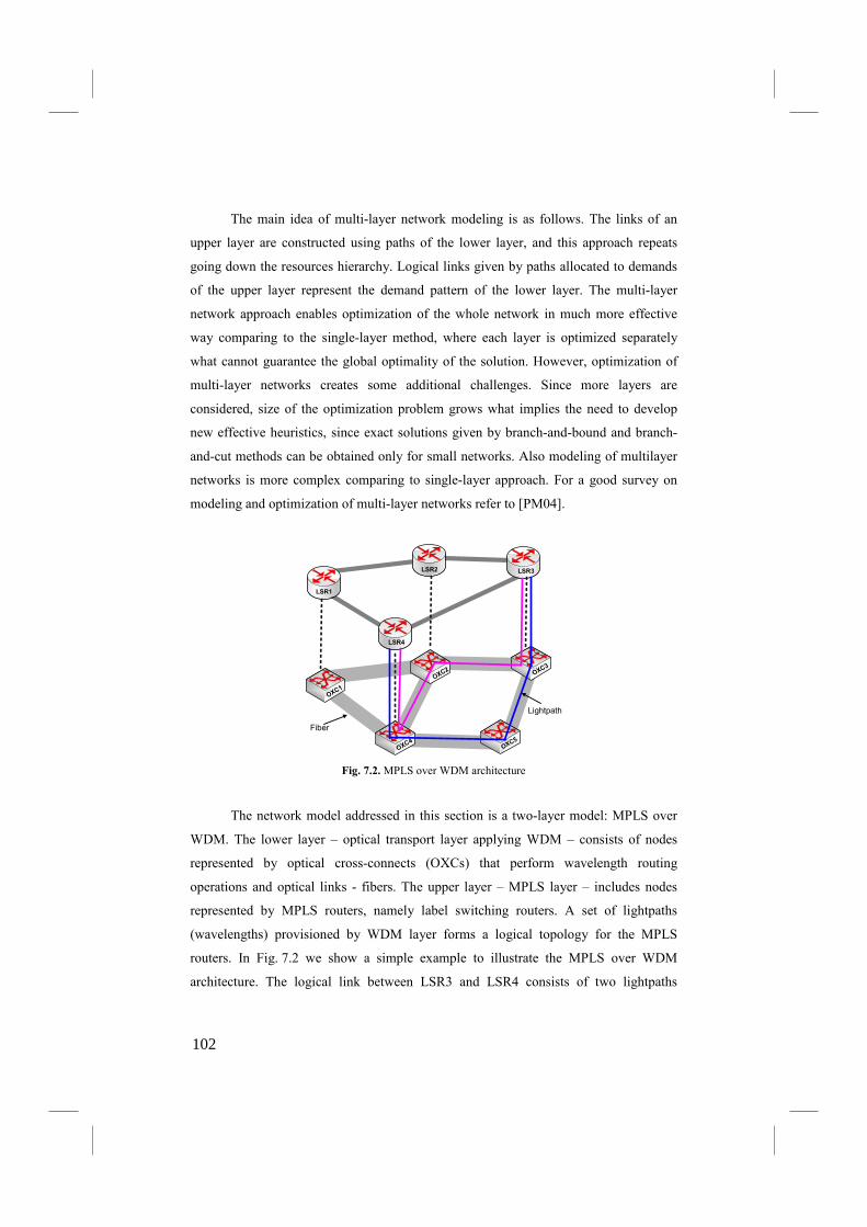
The main idea of multi-layer network modeling is as follows. The links of an
upper layer are constructed using paths of the lower layer, and this approach repeats
going down the resources hierarchy. Logical links given by paths allocated to demands
of the upper layer represent the demand pattern of the lower layer. The multi-layer
network approach enables optimization of the whole network in much more effective
way comparing to the single-layer method, where each layer is optimized separately
what cannot guarantee the global optimality of the solution. However, optimization of
multi-layer networks creates some additional challenges. Since more layers are
considered, size of the optimization problem grows what implies the need to develop
new effective heuristics, since exact solutions given by branch-and-bound and branch-
and-cut methods can be obtained only for small networks. Also modeling of multilayer
networks is more complex comparing to single-layer approach. For a good survey on
modeling and optimization of multi-layer networks refer to [PM04].
LSR3
LSR1
LSR2
LSR4
OXC1
OXC2 OX
C3
OXC4
OXC5
Fiber
Lightpath
Fig. 7.2. MPLS over WDM architecture
The network model addressed in this section is a two-layer model: MPLS over
WDM. The lower layer – optical transport layer applying WDM – consists of nodes
represented by optical cross-connects (OXCs) that perform wavelength routing
operations and optical links - fibers. The upper layer – MPLS layer – includes nodes
represented by MPLS routers, namely label switching routers. A set of lightpaths
(wavelengths) provisioned by WDM layer forms a logical topology for the MPLS
routers. In Fig. 7.2 we show a simple example to illustrate the MPLS over WDM
architecture. The logical link between LSR3 and LSR4 consists of two lightpaths
102

(wavelengths). However, these two lightpaths are routed in two various paths in the
WDM layer: OXC3-OXC5-OXC4 and OXC3-OXC2-OXC4.
The network is modeled as two graphs consisting of nodes and links. Nodes
represent MPLS devices like routers, switches in the upper layer or optical cross-
connects in the lower layer. Links e = 1,2,…,E denote logical links of the MPLS
network. Links g = 1,2,…,G denote physical links of the lower WDM layer, e.g., fibers.
We are given cost of one capacity module on link e in the upper layer ξe, cost of one
module capacity on link g in the lower layer κg and set of connections (unicast and
anycast) denoted by index d = 1,2,…,D. We use the link-path notation in both layers.
We assume that the network topology of both layers, localization of replica servers,
unicast and anycast demand, candidate paths in the upper layer and set of light-paths for
each MPLS logical links are given. Both layers are dimensioned for modular capacity of
links with integral link capacity variables.
Multilayer Unicast and Anycast Design Problem
indices
d = 1,2,…,D demands
d = 1,2,…,A anycast demands (upstream and downstream)
d = A+1,…,D unicast demands
p = 1,2,…,Pd candidate paths for flows realizing demand d. If d is an
upstream demand, path p connects the client node and the
replica node. If d is a downstream demand, candidate
paths connect the replica node and the client node. If d is a
unicast demand, candidate paths connect the origin and
destination nodes of the demand
e = 1,2,…,E network links
q = 1,2,…,Qe candidate paths for link e in lower layer
g = 1,2,…,G network links in lower layer
constants
δedp = 1, if link e belongs to path p realizing demand d; 0, otherwise
ξe cost of one capacity module on link e
M size of the link capacity module in the upper layer
103
γgeq = 1, if link g belongs to path q realizing capacity of link e; 0,
otherwise
κg cost of one capacity module on link e
6 size of the link capacity module in the lower layer
hd volume of unicast demand d
τ(d) index of a demand associated with demand d. If d is a
downstream demand, thenτ(d) must be an upstream connection
and vice versa
s(p) source (origin) node of path p
t(p) destination node of path p
variables
xdp = 1, if path p is used to realize demand d; 0, otherwise (binary)
zeq number of paths q selected to realize capacity of link e
ye capacity of link e as the number of modules (non-negative
integer)
ug number of modules 6 to be installed on link g in the lower layer
(integer, non-negative)
objective
minimize F = ∑e ξeye + ∑g κgug (7.6.1)
subject to
∑p xdp = 1, d = 1,2,…,D (7.6.2)
∑d∑p δedpxdphd ≤ Mye, e = 1,2,…,E (7.6.3)
∑p xdps(p) = ∑p xdτ(p)t(p), d = 1,2,…,A (7.6.4)
∑q zeq = ye, e = 1,2,…,E (7.6.5)
∑e∑q γgeq zeq ≤ 6ug, g = 1,2,…,G. (7.6.6)
The objective (7.6.1) is to minimize the cost of both network layers. Constraint (7.6.2)
assures that only one path can be chosen for each demand (both unicast and anycast)
Condition (7.6.3) states that flow in each link of the upper layer cannot exceed capacity.
Equation (7.6.4) guarantees that paths of two associated anycast demands must connect
the same pair of nodes. Constraint (7.6.5) assures that each upper layer link is realized
by a set of lower layer paths. Finally, condition (7.6.6) states that flow in each link of
104

the lower layer cannot exceed its capacity. For more details on the model and results see
[GW09].
7.7. Exercises
7.1. Write the reduced formulation of anycast flows using the node-link notation.
7.2. Create a branch and bound algorithm for the Unicast and Anycast Delay Problem
(7.2.1)-(7.2.5).
7.3. Write a selected flow allocation problem taking into account unicast, anycast and
multicast flows.
7.4. Write a location, link capacity and flow assignment problem for anycast flows.
7.5. Consider the use of bifurcated multicommodity flows in modeling of anycast flows.
7.6. Write an anycast flow allocation problem with additional traffic required to deliver
the content to replica servers from source sites.
7.7. Write the Multilayer Unicast and Anycast Design Problem using the node-link
notation.
7.8. Construct a computational intelligence algorithm for a selected anycast problem.
105
8. Peer-to-Peer Flows
The concept of Peer-to-Peer (P2P) systems has gained much attention recently. Many
network services including file-sharing, distributed computing, Internet based telephony
(e.g. Skype), Internet television, have been successfully developed using various P2P
mechanisms. According to many statistics, BitTorrent and other P2P systems generate
more than 50% of consumer Internet IP traffic. A great number of research challenges
in the area of P2P is still open, however in this book we focus on modeling and
optimizing of network flows in P2P systems. This challenge follows naturally from the
need to optimize performance of P2P systems from the network perspective.
A P2P system can be defined as a system, in which each node acts both as a
server (producer that provides data to other nodes) and as a client (consumer that
retrieves data from other nodes). Therefore, nodes of P2P systems can be named
“servent”, according to the first syllable of the term Server and the second syllable of
the term Client. P2P systems can be divided to unstructured and structured. Historically,
the first generation of P2P-based systems applied the unstructured approache. The term
“unstructured” follows from the fact that the content stored on a given peer are
unrelated and do not have any specific structure. Unstructured P2P systems can be
categorized as: centralized P2P, pure P2P and hybrid P2P. A centralized P2P system
(e.g., Napster) uses a kind of a central server that stores only information (e.g., IP
addresses) of peers where some content is available. The next category – a pure P2P
system – contains no central server and relies on flooding the information on desired
content over the network (e.g. Gnutella 0.4 and Freenet). A hybrid P2P system employs
a hierarchy of superpeers – servers that store content available to the connected peers
together with their IP address (e.g. Gnutella 0.6 and JXTA). Structured P2P systems are
based on Digital Hash Tables (DHT) that provide a global view of data distributed
among many peers independent of actual location. Each DHT node stores a small of
amount of content that is mapped into nodes by using a special mechanism based on
hashing [BYL09], [SW05], [Tar10].
An interesting example of a P2P-based file distribution system is the BitTorrent
protocol [BYL09], [Coh03], [SW05]. The BitTorrent uses centralized software called
tracker that stores information, which peers have a particular file. To facilitate the
downloading, each file is divided to smaller pieces (e.g., 256 KB). A peer that wants to
download a file can receive from the tracker a random list of peers that contain the file.
106

Then, the downloader requests pieces from all the peers it is connected to. Next, when a
peer downloads some pieces, it can upload them to other peers. Since the main objective
of the system is effective file sharing, peers are encouraged not only to download but
also to upload files. This is achieved by the tit-for-tat strategy. For more information on
P2P systems refer to [BYL09], [SW05], [Tar10] and reference therein.
8.1. Modeling of P2P Flows
P2P flows can be modeled in several ways. In the following section we present two
models of P2P flows:
• Synchronous P2P
• P2P multicast.
Both presented models assume that the P2P system works on the top of an overlay
network and the underlying network is overprovisoned, i.e., the only potential
bottlenecks are access links [ARG08], [MW04]. Furthermore, according to the analysis
presented in [ZL08], nodes’ capacity constraints are typically sufficient in overlay
networks. Nodes (peers) denoted as v = 1,2,…,V are connected to the overlay by an
access links with download capacity dv and upload capacity uv. We consider the access
link as two directed links (download and upload) since in many cases the access link to
the Internet is asymmetric with different capacities in both directions.
The main distinction between both models is related to the time scale. In the
asynchronous modeling the time scale of the P2P system is divided into time slots
t = 1,2,…,T that can be interpreted also as subsequent iterations of the system. We
assume that each time slot has the same length. Moreover, all actions of the P2P system
completed in the previous time slot are updated in such a way that in the beginning of
the next time slots this information is available to all elements of the system. This
follows from the fact that there is an index storing detailed information on current
availability of blocks in the system. Our model is not limited to one exact
implementation of the index, which can be organized in a centralized manner (e.g.
similar to BitTorrent) or decentralized manner (e.g. DHT). Such a P2P system can be
called synchronous [WL08]. Obviously, in real P2P systems peers are mostly
asynchronous, with different processing times and messaging latencies. However, the
assumption on synchronous mode of P2P systems is a common approach in many
research works on P2P modeling [GS05], [KVS05], [MW04], [WL08], [Wal08c],
[Wal08d]. This follows from the fact that modeling and next optimization of
107
asynchronous P2P systems is very difficult in a deterministic way. Data to be sent is
divided into blocks (pieces) indexed b = 1,2,…,B. Transfer of one block is completed
within one time slot. At the end of each time slot (iteration) the indexing service updates
the information on location and availability of blocks. For instance, if block b was
transferred to peer v in time slot t, then all other peers can try to get this block from v in
time slot (t+1). However, the model presented below can be easily modified to include
also more heterogeneous scenarios, e.g. transfer of one block takes more than one slot.
We assume the each block is initially located in a node called seed, and a binary
constant gbv denotes whether or not block b is located in node v before the P2P transfer
starts. A binary variable ybwvt is 1, if block b is transferred to node v from node w in
iteration t and 0 otherwise. In order to meet the requirement that block b can be sent
from node w to node v in time slot t only if node w keeps block b in time slot t we
formulate the following constraint:
∑v ybwvt ≤ M(gbw + ∑i < t∑s ybswi), b = 1,2,…,B w = 1,2,…,V
t = 1,2,…,T. (8.1.1)
where M denotes a large number. Note that the right-hand side of (8.1.1) is a sum of
constant gbw and ∑i < t∑s ybswi (= 1 if block b is transferred to node w from any node s in
any iteration preceding the current time slot t). Consequently, the right-hand side of
(8.1.1) is greater than 0 only if node w holds block b in time slot t. Constraint (8.1.1)
enables the peer-to-peer transfer of blocks. Note that M must be larger than V. As in
[KVS05] we refer to (x.1.1) as possession constraint. Note that the constraint (8.1.1)
defines the P2P flow. The next condition indispensable in model of a P2P system must
guarantee that each peer will receive requesting blocks within all time slots. This can be
written as:
gbv + ∑w∑t ybwvt = 1, b = 1,2,…,B v = 1,2,…,V. (8.1.2)
Notice that since v must posses b either v is the seed of block b (gbv = 1) or block
b is transferred to node v in one of iterations (∑w∑t ybwvt = 1). In (8.1.2) we assume that
each peer v = 1,2,…,V requests all blocks, however it can be easily modify to denote
that a peer wants to download only selected blocks.
As mentioned above, it is a common assumption in modeling and optimization
of overlay network that each node (peer) has a limited capacity of access link to the
network. Let uv denote the maximum upload rate of node v and analogously let dv
108
denote the maximum download rate of node v. If uv and dv are given in bps, constraints
are as follows:
∑b∑v ybwvthb ≤ uw, w = 1,2,…,V t = 1,2,…,T (8.1.3)
∑b∑w ybwvthb ≤ dv, v = 1,2,…,V t = 1,2,…,T. (8.1.4)
where hb denotes the bandwidth required to transfer one block in one time slot given in
bps. For instance, if the block size is 256KB and the duration of one time slot is 16
seconds, then hb = 128Kbps. If we assume that uv and dv are expressed as the number
blocks to be transferred in one time slot, constraints are written in the following way:
∑b∑v ybwvt ≤ uw w = 1,2,…,V t = 1,2,…,T (8.1.5)
∑b∑w ybwvt ≤ dv v = 1,2,…,V t = 1,2,…,T (8.1.6)
For the sake of simplicity in the remainder of this section paper we will assume
that uv and dv are expressed as the number of blocks to be transferred in one time slot.
However, all constraints given below can be easily rewritten according to the approach
presented in (8.1.3)-(8.1.4). The basic version of the synchronous model of P2P systems
can be summarized in the following way.
Synchronous P2P Formulation
indices
b = 1,2,…,B blocks to be transferred
t = 1,2,…,T time slots (iterations)
v,w,s = 1,2,…,V vertices (network nodes, peers)
constants
dv maximum download rate of node v (number of blocks)
uv maximum upload rate of node v (number of blocks)
gbv = 1, if block b is located in node v before the P2P transfer starts;
0, otherwise
M large number
variables
ybwvt = 1, if block b is transferred to node v from node w in iteration t;
0, otherwise (binary)
subject to
gbv + ∑w∑t ybwvt = 1, b = 1,2,…,B v = 1,2,…,V (8.1.7)
109
∑b∑v ybwvt ≤ uw, w = 1,2,…,V t = 1,2,…,T (8.1.8)
∑b∑w ybwvt ≤ dv, v = 1,2,…,V t = 1,2,…,T (8.1.9)
∑v ybwvt ≤ M(gbw + ∑i < t∑s ybswi), b = 1,2,…,B w = 1,2,…,V
t = 1,2,…,T. (8.1.10)
Now we present the P2P multicast formulation. The time scale is modeled as in
traditional multicommodity flow models, i.e., the streaming has a defined rate, constant
in time and given in bps. The term P2P refers in this case to the fact that all peers
(network nodes) are involved in the multicasting. The P2P multicasting (called also
application-layer multicast) uses a multicast delivery tree constructed among peers (end
hosts) using an overlay network. In contrast to the traditional IP multicast (addressed in
Chapter 6), the uploading (non-leaf) nodes in the tree are normal end hosts. Again we
assume that peers are connected to the overlay network, which is considered as an
overprovisioned cloud - capacity constraints are set only on access links. Moreover, the
graph is fully connected, i.e., each peer can connect to any other peer. However, the
model can be modified to introduce some P2P substrate. Various multicast formulations
can be used, e.g., flow formulation or level formulation presented in Section 6.1. The
main modification – comparing to formulation of traditional multicasting presented in
Section 6.1 – is different modeling of capacity constraints and network links. In the
former case, we consider only the capacity of access links (the overlay network is
assumed to be overprovisioned). The latter case means that since the overlay graph is
fully connected, we define the links by origin and destination nodes.
We present the P2P multicast model using the flow formulation. According to
the modification mentioned above, we use a binary variable xwvk to denote if in multicast
tree the streaming path from the root to node k includes an overlay link from node w to
node v (no other peer nodes in between). In analogous way, we assume that xwv is 1, if
the link from node w to node v (no other peer nodes in between) is in multicast tree and
0 otherwise.
P2P Multicast Flow Formulation
indices
v,w = 1,2,…,V network nodes
k = 1,2,…,K terminals (receivers)
110

constants
dv download capacity of node v access link (bps)
uv upload capacity of node v access link (bps)
rv = 1, if link v is the root of streaming; 0, otherwise
h streaming rate
variables
xwvk = 1, if in multicast tree the streaming path from the root to node k
includes an overlay link from node w to node v (no other peer
nodes in between); 0, otherwise (binary)
xwv = 1, if the link from node w to node v (no other peer nodes in
between) is in multicast tree; 0, otherwise (binary)
subject to
∑w xwvk – ∑w xvwk = 1, v = k v = 1,2,…,V k = 1,2,…,K (8.1.11)
∑w xwvk – ∑w xvwk = –1, rv = 1 v = 1,2,…,V k = 1,2,…,K (8.1.12)
∑w xwvk – ∑w xvwk = 0, v ≠ k, rv ≠ 1 v = 1,2,…,V k = 1,2,…,K (8.1.13)
xwvk ≤ xwv, v = 1,2,…,V w = 1,2,…,V k = 1,2,…,K (8.1.14)
∑w xwvh ≤ dv, v = 1,2,…,V (8.1.15)
∑v xwvh ≤ uw, w = 1,2,…,V (8.1.16)
∑v∑t xvvt = 0. (8.1.17)
Constraints (8.1.11)-(8.1.13) define the unicast paths connecting the root node and each
receiver using the node-link formulation of multicommodity flows. Note that in the
above formulation the left-hand side of constraints (8.1.11)-(8.1.13) is the total number
of links entering node v minus the total number of links leaving node v on the unicast
path leading to receiver k. Thus, if the considered node v is the considered receiver node
(v = k), the right-hand side must be 1 (8.1.11). On the other hand, if the node v is the
root node (rv = 1), the right-hand side must be –1 (8.1.12). Ale remaining nodes are
transit nodes, and the flow balance must be 0 (8.1.13). Constraint (8.1.14) assures that
each overlay link (w,v) is used in the multicast at most one time. (8.1.15) and (8.1.16)
are the download and upload constraints, respectively. Note that the left-hand side of
(8.1.15) is the sum of the multicast flow entering node v (from any other node w).
Analogously, the left-hand side of (8.1.16) is the total flow leaving node w to any other
111

node v. Finally, the last constraint (8.1.17) guarantees that there is no internal flow
inside each node.
8.2. Synchronous P2P Cost Problem
Now we present a synchronous P2P model with the objective to minimize the transfer
cost. Currently used P2P systems mostly ignore the underlying Internet topology and
ISP link costs, since they are designed to randomly choose logical neighbors. Thus,
there are many cross-continental downloads that can congest backbone networks. In
order to estimate the transfer cost, it is necessary to provide an effective mechanism for
localization of peers by using for instance: IP location databases, IP prefix, traceroute
records, hop number and RTT (round-trip time). In the model we introduce a universal
constant ζwv that is defined as the cost of one block transfer between peers w and v. It
can be interpreted arbitrarily according to our needs, e.g. number of hops between w and
v, number of ISPs between w and v, RTT between w and v, distance in kilometers
between w and v, cost of cross-ISP transfers, etc. Consequently, the objective (to be
minimized) is formulated as F = ∑b∑w∑v∑t ybwvt ζwv, i.e., all possible transfers are
considered taking into account of node pairs, time slots and blocks [Wal08c], [Wal08d].
An important characteristic of P2P systems is dynamics – peers can frequently
join or leave the network. To model this phenomenon in our approach we use constants
avt, which equals 1 if peer v in time slot t is connected to the network (is available) and 0
otherwise. Consequently, although our model is deterministic, the stochastic nature of
P2P system can be incorporated into our considerations [Wal08c], [Wal08d].
Synchronous P2P Cost Problem
indices
b = 1,2,…,B blocks to be transferred
t = 1,2,…,T time slots (iterations)
v,w,s = 1,2,…,V vertices (network nodes, peers)
constants
dv maximum download rate of node v (number of blocks)
uv maximum upload rate of node v (number of blocks)
gbv = 1, if block b is located in node v before the P2P transfer starts;
0, otherwise
112
avt = 1, if node v is available in time slot t; 0, otherwise
M large number
variables
ybwvt = 1, if block b is transferred to node v from node w in iteration t;
0, otherwise (binary)
objective
minimize F = ∑b∑w∑v∑t ybwvt ζwv (8.2.1)
subject to
gbv + ∑w∑t ybwvt = 1, b = 1,2,…,B v = 1,2,…,V (8.2.2)
∑b∑v ybwvt ≤ awtuw, w = 1,2,…,V t = 1,2,…,T (8.2.3)
∑b∑w ybwvt ≤ avtdv, v = 1,2,…,V t = 1,2,…,T (8.2.4)
∑v ybwvt ≤ M(gbw + ∑i < t∑s ybswi), b = 1,2,…,B w = 1,2,…,V
t = 1,2,…,T. (8.2.5)
The objective function (8.2.1) is the cost of block transfer using the P2P approach. To
meet the requirement that each block must be transported to each network node we
introduce the condition (8.2.2). Constraint (8.2.3) assures that the number of blocks
uploaded by node w can not exceed a given threshold. Analogously, (8.2.4) bounds the
download rate of node v. The constant avt used on the right-hand side of (8.2.3) and
(8.2.4) enables to incorporate to the model stochastic nature of P2P clients that can
frequently join and leave the network. Construction of (8.2.3) and (8.2.4) guarantees
that if a peer v is not connected to the P2P network in iteration t (avt = 0) then v cannot
upload and download any blocks in this time slot. Possession constraint (8.2.5) is in the
model to meet the requirement that block b can be sent from node w to node v only if
node w keeps block b in time slot t. The problem (8.2.1)-(8.2.5) is linear, integer
(binary) and NP-complete (equivalent to MBT (Minimum Broadcast Time) problem).
To solve the Synchronous P2P Cost Problem we propose a heuristic algorithm
that we developed in [Wal08d] to simulate a real BitTorrent-like P2P system. Our
approach follows mainly from the BitTorrent protocol [Coh03], [SW05] and ideas
included in [GS05], [WLH07] and [YTM07]. However, some simplifications had to be
made in order to adjust the heuristic to the considered optimization model. Since the
goal of our research is to examine transfer cost aspects of P2P systems, we do not
simulate all details – it is sufficient to mirror only the major characteristics of the
113

BitTorrent-like P2P system. Fig. 8.1 presents the outline of the algorithm in
pseudocode.
1 for t=0 to T 2 begin
3 while (IsPossibleTranfer(t)) 4 begin 5 v=RandomDownloadPeer(t)
6 b=SelectBlock(v,t) 7 w=SelectUploadPeer(b,v,t)
8 TransferBlock(b,w,v,t) 9 end (if) 10 end (for)
Fig. 8.1. Pseudocode of the P2P transfer algorithm
Since our model is synchronous, i.e., the system works in iterations, the main
loop of the algorithm (lines 1-10) is repeated for each time slot t. Function
IsPossibleTranfer(t) (line 3) returns 1, if there is a possible transfer in the P2P
system, i.e., at least one block b can be transferred from a node w possessing block b to
node v requesting block b not violating the constraints of the system (i.e. limits on
upload and download capacity, possession of the block, availability of peers, etc.).
Otherwise function IsPossibleTranfer(t) returns 0. The inner loop (lines 3-9) is
repeated until there is at least one possible block transfer.
To model the stochastic nature of BitTorrent-like P2P system, we randomly
select the download peer among all feasible peers (line 5). A download peer v is feasible
if it can upload at least one block from other peer satisfying all constraints of the
system. Next, a block to be transferred is chosen among all feasible blocks (line 6). A
block b is feasible if at least one node can upload this block to v satisfying all
constraints of the system. Finally, the uploading peer is selected among all feasible
upload peers (line 7). As previously, upload node w is feasible if it can upload block b
to v satisfying all constraints of the system. Function TransferBlock(b,w,v,t)
(line 8) transfers block b from w to v and updates state of the P2P system (upload and
download limits, possession of the block, etc.).
We consider 4 versions of the algorithm. Thus, functions
SelectBlock(b,v) and SelectUploadPeer(b,v,t) have different versions
according to a particular strategy. The first algorithm – Random Strategy (RS) – selects
the block (line 6) and upload peer (7) at random among all feasible blocks and upload
nodes. To model the second strategy named Rarest First Strategy (RFS) function
114
SelectBlock (line 6) returns the rarest feasible block in the network. Next, the
upload peer is chosen at random. The third approach – Cost Selection Strategy (CSS) –
takes into account transfer costs. The block to be transferred is selected at random (line
6), but the closest (in terms of the cost), feasible peer is chosen for upload. Finally, we
also model the Weighty Piece Selection Strategy (WPSS) as in [WLH07]. For results of
the proposed algorithm and comparison to optimal solutions refer to [Wal08c] and
[Wal08d].
8.3. Other Formulations of Synchronous P2P Problems
The synchronous P2P model (8.1.7)-(8.1.10) can use also other objective functions.
First, we address the problem to minimize the overall download time, i.e., the time in
which all requesting peers receive requested blocks [GS05], [MW04], [SW05],
[WLH07], [Wal08c]. In the synchronous P2P model the download time is represented
by T – a constant denoting the number of time slots. Note that if T is used as the
objective function, the problem becomes a Non-linear Integer Problem, which cannot be
solved by classical branch and bound algorithms included in optimizers like CPLEX.
However, the following procedure can be employed to find the minimal value of T.
First, set T to some value. Solve the optimization problem consisting of P2P system
constraints. If the problem has a feasible solution, then decrease T by 1; otherwise
increase T by 1.
Another approach to minimize the number of time slots required to transfer all
blocks is as follows. Let us introduce an additional binary variable xt, which is 1 if in
time slot t there is at least one transfer; 0 otherwise (binary). To find variables xt we use
the following condition:
∑b∑w∑v ybwvt ≤ M xt, t = 1,2,…,T. (8.3.1)
Notice that the left-hand side of (8.3.1) is larger then 0, if there is at least one
transfer in time slot t, thus variable xt must be 1. Finally, we can write the objective to
be minimized as ∑t xt.
Another possible objective function is throughput of the P2P system, which is
defined as the number of blocks (which can be interpreted as the size of a file) that can
be transferred to every peer within given time (number of time slots). The procedure to
solve the problem with the throughput objective can be the same as in the case of the
download time.
115
Many P2P systems try to avoid the selfishness of the users, thus mechanisms to
provide the fairness are required [SW05], [Wal08c]. The idea is to ensure that the
number of blocks downloaded by each peer is comparable to the number of uploads. Of
course peers acting as seed can have got asymmetries. Fairness can be viewed as a kind
of an incentive for nodes to participate, especially in situations where ISPs charge based
on uplink usage or uplink bandwidth is scarce. To enforce fairness in the P2P system we
add the following constraints for each node v:
∑b∑w∑t ybvwt ≤ Ψ ∑b∑w∑t ybwvt, v = 1,2,…,V. (8.3.2)
The left-hand side of (8.3.2) denotes the number of blocks uploaded by v in all
considered time slots. Analogously, the right-hand side is the number of blocks
downloaded by v in all considered time slots. Constant Ψ denotes the fairness of the
system that must be accomplished. Peers acting as the seed can be excluded from
constraint (8.3.2). Note that condition (8.3.2) assures that the level of fairness is
completed for each peer. Another possible formulation assumes that the average
fairness of all peers must be under a particular level given by Ψ:
∑b∑v∑w∑t ybvwt ≤ Ψ ∑b∑w∑v∑t ybvwt, v = 1,2,…,V. (8.3.3)
In the BitTorrent protocol a new peer joining the system asks the tracker for a
list of peers to connect to and cooperate with (exchange blocks). Such peers are called
neighbors [Coh03], [SW05], [Wal08c]. To model this we introduce a constant ewv which
equals 1 if peers w and v are neighbors, 0 otherwise. Next a following condition can be
formulated:
∑b∑t ybwvt ≤ Mewv, w = 1,2,…,V v = 1,2,…,V. (x.3.4)
Note that the left-hand side of (8.3.4) denotes the number of block transfers in
all time slots between peers w and v. Objective functions and additional constraints
presented in this section can be added to the basic synchronous model P2P to construct
a more sophisticated problem.
8.4. P2P Multicast Network Design Problem
In this section we address a network design problem for P2P multicasting [Wal09a],
[Wal10b]. Simply put, for the given streaming rate we want to determine how much
resource capacity is needed for each peer and how to economically distribute the
streaming content in the overlay network using P2P multicasting. The former goal
consists in selection of one access link type among options proposed by the ISP selected
116
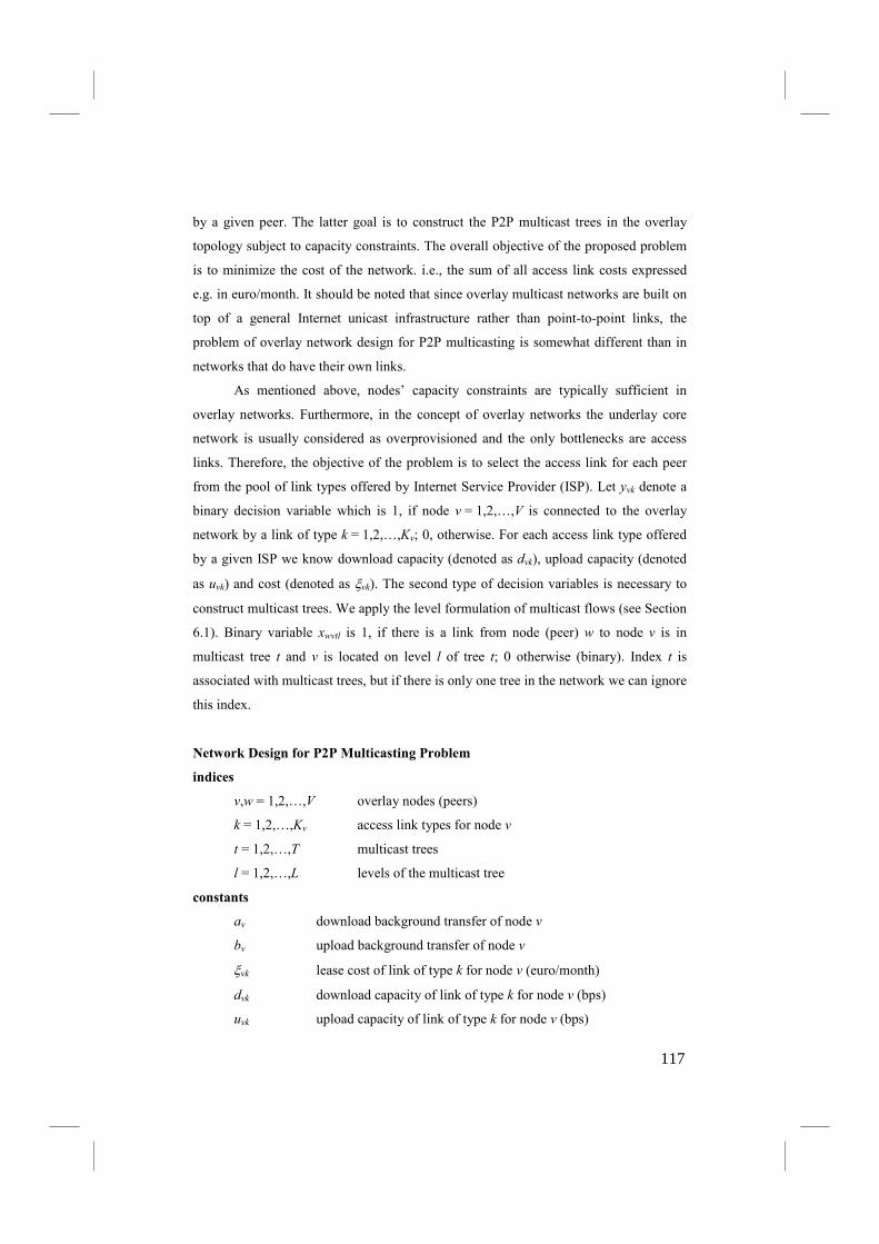
by a given peer. The latter goal is to construct the P2P multicast trees in the overlay
topology subject to capacity constraints. The overall objective of the proposed problem
is to minimize the cost of the network. i.e., the sum of all access link costs expressed
e.g. in euro/month. It should be noted that since overlay multicast networks are built on
top of a general Internet unicast infrastructure rather than point-to-point links, the
problem of overlay network design for P2P multicasting is somewhat different than in
networks that do have their own links.
As mentioned above, nodes’ capacity constraints are typically sufficient in
overlay networks. Furthermore, in the concept of overlay networks the underlay core
network is usually considered as overprovisioned and the only bottlenecks are access
links. Therefore, the objective of the problem is to select the access link for each peer
from the pool of link types offered by Internet Service Provider (ISP). Let yvk denote a
binary decision variable which is 1, if node v = 1,2,…,V is connected to the overlay
network by a link of type k = 1,2,…,Kv; 0, otherwise. For each access link type offered
by a given ISP we know download capacity (denoted as dvk), upload capacity (denoted
as uvk) and cost (denoted as ξvk). The second type of decision variables is necessary to
construct multicast trees. We apply the level formulation of multicast flows (see Section
6.1). Binary variable xwvtl is 1, if there is a link from node (peer) w to node v is in
multicast tree t and v is located on level l of tree t; 0 otherwise (binary). Index t is
associated with multicast trees, but if there is only one tree in the network we can ignore
this index.
�etwork Design for P2P Multicasting Problem
indices
v,w = 1,2,…,V overlay nodes (peers)
k = 1,2,…,Kv access link types for node v
t = 1,2,…,T multicast trees
l = 1,2,…,L levels of the multicast tree
constants
av download background transfer of node v
bv upload background transfer of node v
ξvk lease cost of link of type k for node v (euro/month)
dvk download capacity of link of type k for node v (bps)
uvk upload capacity of link of type k for node v (bps)
117
rv = 1, if node v is the root of all trees; 0, otherwise
qt streaming rate of tree t (bps)
M large number
variables
xvwtl = 1, if in the multicast tree t there is a link from the node v to the
node w and v is located on the level l of tree t; 0, otherwise
(binary)
yvk = 1, if the node v is connected to the overlay network by a link of
type k; 0, otherwise (binary)
objective
minimize F = ∑v∑k yvk ξvk (8.4.1)
subject to
∑v≠w∑l xvwtl = (1 – rw), w = 1,2,…,V t = 1,2,…,T (8.4.2)
∑w≠v∑t xvwt1 ≤ M rv, v = 1,2,…,V (8.4.3)
∑w≠v xvwt(l+1) ≤ M ∑w≠v xwvtl, v = 1,2,…,V t = 1,2,…,T
l = 1,2,…,L – 1 (8.4.4)
∑k yvk = 1, v = 1,2,…,V (8.4.5)
av + ∑t qt ≤ ∑k yvk dvk, v = 1,2,…,V (8.4.6)
bv + ∑w≠v∑t∑l xvwtl qt ≤ ∑k yvk uvk, v = 1,2,…,V. (8.4.7)
The objective function (8.4.1) is the overall cost of access links of the overlay network.
Since for each tree t = 1,2,…,T each node w = 1,2,…,V – except the source node of the
tree (rw = 1) – must have exactly one parent node, we use constraint (8.4.2). Condition
(8.4.3) guarantees that node v can be the parent of the first level link, only if it is the
root node. Constraint (8.4.4) is in the model to meet the requirement that each node
v = 1,2,…,V cannot be a parent on level (l + 1) if it is not a child on the level l.
Constraint (8.4.5) assures that one access link is selected for each overlay node.
Condition (8.4.6) is a download capacity constraint, i.e. the streaming rate of all trees
and the download background traffic cannot exceed the download capacity of each
node. Correspondingly, (8.4.7) is the upload capacity constraint.
Now we show a heuristic algorithm for the problem (8.4.1)-(8.4.7) proposed in
[Wal10b]. Without loss of generality we assume that for each node v = 1,2,…,V the
access link types are sorted according to the increasing values of upload capacity and
118

cost. All functions and operators presented below are executed using the current state of
the problem, i.e. the current values of decision variables, which in effect yield current
network flows and access links’ capacity. To formulate the algorithm we introduce the
following definitions:
• Transfer between node v and node w is possible in tree t on level l if node v is
located in tree t on level l; node w is not yet connected to tree t; node v has enough
upload residual capacity to stream the rate of tree t.
• Tree t is feasible on level l if there is at least one possible transfer from node v
(located on level l of tree t) to node w.
• Let ftree(l) return an index of a feasible tree on level l. If there is more than one
feasible tree, we select the tree with the lowest number of nodes connected to the
tree.
• Node v is a feasible parent node on level l of tree t if there is at least one possible
transfer in tree t on level l between v and any other node.
• Let fpnode(t, l) return an index of a feasible parent node located on level l of tree
t. If there is more than one feasible parent node, the algorithm chooses the node
with the largest value of residual upload capacity. Notice that if l = 1, fpnode(t, l)
returns always the index of the root node.
• Let fcnode(v, t, l) return an index of a feasible child node of node v located on
level l of tree t . If there is more than one feasible child node, again the residual
upload capacity is the additional criterion.
• Let istrasnfer(l) return 1 if there is at least one possible transfer on level l of any
tree, 0 otherwise.
• If each node v = 1,2,…,V is connected to each tree t = 1,2,…,T, i.e. all necessary
transfers are completed, function istree() returns 1; otherwise it returns 0.
• Function isupdate() returns 1 if incrementing of the access link upload capacity is
possible for at least one node; 0 otherwise.
• Let function updatenode() return an index of a node v, for which the upload
capacity can be augmented. If there is more than one such a node, an additional
criterion is applied. In the algorithm we use several combinations of two values:
node level and relative cost of upload capacity increase given by the formula
(uv(k+1) – uvk) / (ξv(k+1) – ξvk).
119

• We assume that first(A) returns the first element of table A. Let q = ∑t qt denote
the overall streaming tree rate of all trees.
Algorithm CreateTree
Step 0. Set xvwtl = 0 for each v = 1,2,…,V, w = 1,2,…,V, t = 1,2,…,T, l = 1,2,…,L, v ≠ w.
Set yvk as the minimal values that guarantee sufficient download capacity for
each node v expect the root node (i.e. dvk ≥ av + q) and the sufficient upload
capacity for the root node r (i.e. urj ≥ br + q).
Step 1. Set l = 1. Create table A containing all trees sorted in decreasing order of
streaming rate qt. Create table B containing all nodes except the root node sorted
in decreasing order of residual upload capacity of each node.
a) If A = ∅ go to Step 2. Otherwise, go to Step 1b.
b) Calculate t = first(A), w = first(B) and xrwtl = 1. Next, set A = A – {t} and
B = B – {w}. Go to Step 1a.
Step 2. If l > L go to step 3.
a) If istrasnfer(l) = 0 set l = l + 1 and go to Step 2. Otherwise go to Step 2b.
b) Set t = ftree(l), v = fpnode(t, l), w = fcnode(v, t, l) and xvwtl = 1. Go to Step 2a.
Step 3. If istree() = 1 stop the algorithm, a feasible solution exists. Otherwise, go to
Step 4.
Step 4. If isupdate() = 0, stop the algorithm, there is not feasible solution. Otherwise, go
to Step 5.
Step 5. Set v = updatenode(). Find k, for which yvk = 1. Set yvk = 0, k = k + 1, yvk = 1,
l = 1 and go to Step 2.
We start with an initialization of all variables xvwtl and yvk (Step 0). The idea behind the
selection of variables yvk is to find for each node a link that has sufficient download
capacity to transmit the background traffic and the overall streaming rate of all multicast
trees. Only for the root node additional procedure is run to ensure satisfactory upload
capacity. Next, in Step 1 we ensure that in each tree t = 1,2,…,T there is at least one link
from the root node to another node with possible large residual upload capacity. Step 2
creates multicast trees denoted by variables xvwtl. The main loop of Step 2 is repeated for
subsequent tree levels to allocate resources of upload capacity proportionally to all
trees. If after Step 2 all nodes are connected to each tree, the algorithm exits (Step 3).
120
Otherwise, there is an attempt to increase capacity of the access link of a selected node
(Step 4 and 5). For results of the Create Tree algorithm refer to [Wal10b]. Note that in
[Wal09a] we developed a Lagrangean relaxation algorithm for the above problem.
8.5. Survivable P2P Multicasting
Network survivability is significant research topic in recent years, since a network
failure could cause a lot of damages including economic loses, political conflicts,
human health problems. Most of previous research has been focusing on networks using
unicast flows (e.g., see [Gro04], [PM04]). Now we want to address the problem of
survivability in the context of P2P multicasting system. The model presented below was
formulated and evaluated in [Wal09b]. To protect the P2P multicasting system we
propose to use an approach similar to 1:1 protection [Gro04] and establish two (or
more) failure disjoint P2P multicast trees streaming the same content. We take into
account three kinds of network failures: overlay link failure, uploading node failure and
ISP link failure. For the overlay link failure, a pair of peers is disconnected. If there was
a transfer on this link, some downstream nodes are affected by the failure. The overlay
link failure comprises failure of both directed links. This follows from the fact that
usually a network failure influences the transfer in both directions. The second failure –
uploading node failure – impacts all successors of the failed peer in the tree. Therefore,
we focus only on failure of nodes that have some children. Leaf node failure affects
only this one node. The P2P multicasting is usually used in the Internet, which consists
of many ISP operators. Each peer is connected to a particular ISP. A failure of cross ISP
link means, that all overlay links between peers of one ISP and peers of the second ISP
are not available.
In Fig. 8.2a we present a simple example to illustrate our concept. Two trees A
and B are established in the overlay network connecting 8 nodes a, b, c, d, e, f, g, h. Peer
a is the root of tree A and peer b is the root of tree B. Other nodes c, d, e, f, g, h are
receivers of the signal. In the case of tree A nodes a, c and f are uploading (non-leaf)
nodes, while the remaining nodes d, e, g, h are leafs. Nodes a, c, d and e belong to ISP
1. Nodes b, f, g and h are assigned to ISP 2. We use the term of level to describe the
nodes. For instance, the node a is on level 1 of tree A, nodes c and f are on level 2 of
tree A, nodes d, e, g and h are on level 3. The tree A has 3 levels of nodes and the tree B
is of 4 levels. Notice that the overlay link (c,d) belongs to both trees, so in the
consequence of link (c,d) failure, the node d will be connected to none tree. Peer c is an
121
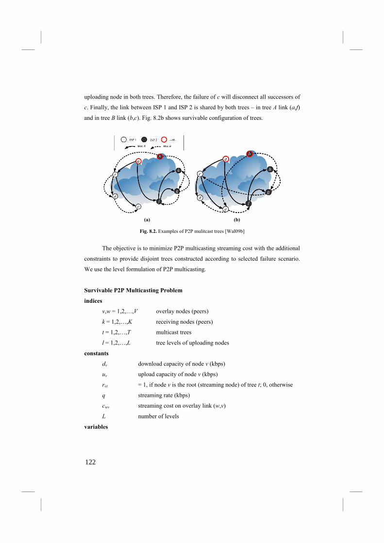
uploading node in both trees. Therefore, the failure of c will disconnect all successors of
c. Finally, the link between ISP 1 and ISP 2 is shared by both trees – in tree A link (a,f)
and in tree B link (b,c). Fig. 8.2b shows survivable configuration of trees.
(a) (b)
Fig. 8.2. Examples of P2P mulitcast trees [Wal09b]
The objective is to minimize P2P multicasting streaming cost with the additional
constraints to provide disjoint trees constructed according to selected failure scenario.
We use the level formulation of P2P multicasting.
Survivable P2P Multicasting Problem
indices
v,w = 1,2,…,V overlay nodes (peers)
k = 1,2,…,K receiving nodes (peers)
t = 1,2,…,T multicast trees
l = 1,2,…,L tree levels of uploading nodes
constants
dv download capacity of node v (kbps)
uv upload capacity of node v (kbps)
rvt = 1, if node v is the root (streaming node) of tree t; 0, otherwise
q streaming rate (kbps)
cwv streaming cost on overlay link (w,v)
L number of levels
variables
122
xwvtl streaming rate on an overlay link (w,v) (no other peer nodes in
between) in multicast tree t and w is located on level l of tree t;
(continuous, non-negative)
ywvt = 1, if the link from node w to node v (no other peer nodes in
between) is in multicast tree t; 0, otherwise; (binary)
objective
minimize ∑w∑v∑t ywvtcwv (8.5.1)
constraints
∑w∑t∑l xwvtl = 0, v = 1,2,…,V t = 1,2,…,T rvt = 1 (8.5.2)
∑w∑l xwktl = q, k = 1,2,…,K t = 1,2,…,T (8.5.3)
∑v xwvt1 ≤ uw rwt, w = 1,2,…,V t = 1,2,…,T (8.5.4)
xwvt(l+1) ≤ ∑b xbwtl, v = 1,2,…,V w = 1,2,…,v
t = 1,2,…,T l = 1,2,…,L – 1 (8.5.5)
∑w∑t∑l xwvtl ≤ dv, v = 1,2,…,V (8.5.6)
∑v∑t∑l xwvtl ≤ uv, w = 1,2,…,V (8.5.7)
∑v∑t∑l xvvtl =0, (8.5.8)
∑l xwvtl ≤ qywvt, v = 1,2,…,V w = 1,2,…,v t = 1,2,…,T (8.5.9)
ywvt ≤ ∑l xwvtl, v = 1,2,…,V w = 1,2,…,v t = 1,2,…,T (8.5.10)
∑w ywkt = 1, k = 1,2,…,K t = 1,2,…,T. (8.5.11)
The criterion function (8.5.1) is the streaming cost. Condition (8.5.2) assures the
download flow to be zero for the root node of each tree. Constraint (8.5.3) guarantees
that each receiving node k = 1,2,…,K must be connected to each streaming tree. To
meet the requirement that a node w can be the parent of the first level link in tree t, only
if it is the root node (rwt = 1) we add constraint (8.5.4). Condition (8.5.5) is in the model
to assure that each node w cannot upload to any other peer v on level (l + 1) more than it
downloads on level l. (8.5.6) and (8.5.7) are download and upload capacity constraints,
respectively. Constraint (8.5.8) guarantees that the node internal flow is zero. To bind
variable xwvtl and ywvt we use constraints (8.5.9) and (8.5.10). Finally, condition (8.5.11)
assures that each receiving peer has exactly one parent node.
Now we formulate additional constraints that are related to survivability of P2P
multicasting. Using the basic formulation (8.5.1)-(8.5.11) we show how to model the
123

following three scenarios: overlay link failure, uploading node failure and ISP link
failure. We use the same notation as in the previous section.
The first model protects the P2P multicasting against the single overlay link
failure.
Link Disjoint (LD)
constraints (additional)
∑t (ywvt + yvwt) ≤ 1, v = 1,2,…,V w = 1,2,…,V v < w. (8.5.12)
Notice that in the case of the overlay link failure both directed links ((w,v) and (v,w))
are broken. This follows from the fact that usually a network failure influences the
transfer in both directions.
Next we formulate additional constraints for the uploading node failure. We use
additional binary variable yvt denoting if a particular node is uploading in tree t.
�ode Disjoint (�D)
variables (additional)
yvt =1, if node v is uploading in multicast tree t; 0, otherwise (binary)
constraints (additional)
∑v ywvt ≤ Mywt, w = 1,2,…,V t = 1,2,…,T (8.5.13)
ywt ≤ ∑v ywvt, w = 1,2,…,V t = 1,2,…,T (8.5.14)
∑t yvt ≤ 1, v = 1,2,…,V. (8.5.15)
Finally, we present a model related to the ISP link failure. A new binary variable zpmt is
1, if in tree t there is at least one link from a peer located in ISP p to a peer located in
ISP m or in opposite direction; 0, otherwise.
ISP Link Disjoint (ID)
indices (additional)
p,m = 1,2,…,P Internet Service Providers (ISPs)
constants (additional)
α(v,p) = 1, if node v belongs to ISP p; 0, otherwise
variables (additional)
124
zpmt = 1, if in multicast tree t there is at least one link from a node located in
ISP p to a node located in ISP m or in opposite direction; 0, otherwise (binary)
constraints (additional)
∑w:α(w,p)=1∑v:α(v,m)=1 (ywvt + yvwt) ≤ Mzpmt, p = 1,2,…,P
m = 1,2,…,P p ≠ m t = 1,2,…,T (8.5.16)
zpmt ≤ ∑w:α(w,p)=1∑v:α(v,m)=1 (ywvt + yvwt), p = 1,2,…,P
m = 1,2,…,P p ≠ m t = 1,2,…,T (8.5.17)
∑t zpmt ≤ 1, p = 1,2,…,P m = 1,2,…,P. (8.5.18)
Note that analogous to the overlay link failure case, the ISP link failure includes the
failure of both directed ISP links, i.e., (p,m) and (m,p). For more details on the model
and results see [Wal09b].
8.6. Exercises
8.1. How to modify constraint (8.1.2) to denote that a peer wants to download only
selected blocks?
8.2. Calculate the complexity (number of variables and constraints) of the synchronous
P2P formulation.
8.3. Write the P2P multicasting model using the level formulation.
8.4. Propose an additional constraint for a P2P system following from real systems. Use
the synchronous P2P modeling.
8.5. Write the root location problem for the P2P synchronous modeling.
8.6. Write the root location problem for the P2P multicasting modeling.
8.7. Write the Survivable P2P Multicasting Problem using the flow notation. Compare
the model size (number of variables and constraints) between both formulations.
8.8. Construct a computational intelligence algorithm for a selected P2P problem.
125
9. Distributed Computing Systems
Distributed computing systems have been becoming very important and popular in both
academia and industry, due to the growing need for various kinds of excessive
computations related for instance to: financial modeling, medical data analysis,
experimental data acquisition, earthquake simulation, and climate/weather modeling,
astrophysics and many others [MKL02], [NSW04]. Therefore, the approach of grid
computing appeared in mid-1990s partially replacing previously dominating
supercomputers. Distributed computing systems contain many computers connected to
one computational system, which is considered as one virtual machine with a large
computation power. Thus, such systems can be used to process tasks requiring huge
computation power not available on a single machine (even on a super-computer).
Distributed computing systems are mainly divided into two categories:
• Grid computing systems. According to [FI03] the grid is defined as a sharing
environment implemented by the deployment of a persistent, standards-based
service infrastructure that enables creation and resource sharing within
distributed communities. Grids can include the following resources: computers,
storage space, sensors, software applications and data. All elements of the grid
are connected through the Internet. One of the primary goals of grids was to
enable resource sharing within scientific collaboration, currently there are some
efforts towards grid resource commercialization [FI03], [NSW04].
• P2P (Peer-to-Peer) computing systems called also public resource or global
computing systems are focused mainly on the application of personal
computers (e.g., PC or Macintosh) and other relatively simple electronic
equipment instead of supercomputers and clusters [AB04], [MKL02]. The
well-known example of public-resource computing project is SETI@home
started in the 1999 [ACK02]. SETI@home has been developed using BOINC
(Berkeley Open Infrastructure for Network Computing) software.
Although public-resource computing and Grid computing systems are designed to the
same goal of better utilizing various computing resources, there are differences in many
aspects between these two approaches. First, grids assume more formal organization –
elements of the grid (supercomputers, clusters, research labs, companies) are centrally
managed, permanently available online, connected by high bandwidth network links. In
contrast, participants of public-resource computing projects are individuals with PCs
126

connected to the Internet by DSL access links. Computers can be powered off or
disconnected from the Internet [Wal08e], [AB04].
Since Grids and public-resource computing systems are mostly implemented in a
distributed manner, networks – especially the Internet – have been always indispensable
to both computing approaches. According to [NSW04] communication-intensive Grid
applications require networks for transferring large amount of input and output data.
Characteristics of the generated network traffic depend on particular applications and
workflow of the computational projects. Usually an overlay network model is used – the
underlying physical network is assumed to be a cloud that provides network services
and connectivity. Another example of distributed computing system that gains much
attention recently is the concept of cloud computing – a dynamically scalable and
usually virtualized environment that provides various services over the Internet.
9.1. Overlay Cost Problem
First, we consider an optimization problem related to a distributed computing system
working in the overlay mode with the objective to minimize the operating cost
[WW09], [KWW10]. The network computing system consists of clusters – represented
as nodes v = 1,2,…,V – connected to the overlay network. Each node is described by the
download and upload capacity denoted as dv and uv, respectively. The maximum
processing rate of node v, i.e., the number of uniform computational tasks that node v
can calculate in one second is denoted as pv. Furthermore, we are given ψv – the
processing cost of one computational uniform task in node v. The transfer cost between
nodes w and v is denoted by ζwv. In the network computing systems a set of
computational projects r = 1,2,…,R are to be computed. Each project is described by the
following parameters. The number of uniform computational tasks in project r is
denoted by nr. Each project has a source node that produces the input data and one or
more destination nodes that want to receive the output data, i.e. results of computations.
For simplicity we assume that the uniform task for each project has the same
computational requirement expressed in FLOPS. However, the values of the input and
the output data transmit rate are specific for each computational project following from
particular features of the project. Constants ar and br denote the transmit rate of input
data and output data, respectively, per one task in project r and are given in bps.
The workflow of computational tasks is as follows. The input data is transferred
from the source node to one or more computing nodes that process the data. Next, the
127
output data is sent from the computing node to one or more destination nodes. We
assume that the computational project is long-lived, i.e., it is established for a relatively
long time (days, weeks). As a result, the input and the output data associated with the
project is continuously generated and transmitted. Consequently, computational and
network resources can be reserved in the system according to offline optimization. The
decision variable xrv is integer and denotes the number of project r tasks computed on
node v. The objective cost function includes two elements: the processing cost of tasks
the transmit cost. The processing cost can include all aspects of IT infrastructure
(energy, maintaining, hardware amortization etc.). The second element of the cost
function is the transmission cost ζwv between nodes w and v. We propose several
interpretations of this value. Firstly, let ζwv denote the distance (in kilometers) between
w and v. In the concept of overlay network usually the underlay core network is
considered as overprovisioned and the only bottlenecks are access links. But, selfish use
of the network resources can lead in some cases to network congestion. Therefore, we
propose to minimize the network traffic generated in the overlay network. The second
explanation is also network related – let ζwv denote the network latency between vertices
w and v. The motivation is comparable to the previous case, i.e., a network path with
lower latency is usually less overloaded and minimization of the overall network
latency should decrease network congestion. The last explanation of ζwv is an
economical one. For instance, if ζw and ζv are unit costs of access links of node w and v,
respectively, we can compute ζwv = (ζw + ζv)/2. The ζv can be related to the service
charge of the access link per month or maintenance costs.
Overlay Cost Problem
indices
v,w = 1,2,…,V overlay nodes (peers)
r = 1,2,…,R projects
constants
pv maximum processing rate of node v (number of computational
tasks that node v can calculate in one second)
dv download capacity of node v (bps)
uv upload capacity of node v (bps)
nr number of tasks in project r
128
ar transmit rate of input data per one task in project r (bps)
br transmit rate of output data per one task in project r (bps)
s(r,v) = 1, if v is the source node of project r; 0, otherwise
t(r,v) = 1, if v is the destination node of project r; 0, otherwise
ψv processing cost of one computational task in node v
ζwv transfer cost of 1 bps from node w to node v
M large number
variables
xrv the number of tasks of project r calculated on node v (integer)
objective
minimize F = ∑r∑v xrvψv + ∑r∑w:s(r,w)=1 ∑v:v≠w arxrvζwv +
∑r∑w:t(r,w)=1 ∑v:v≠w brxrvζvw (9.1.1)
subject to
∑r xrv ≤ pv, v = 1,2,…,V (9.1.2)
∑r (1 – s(r,v))arxrv + ∑r:t(r,v)=1 br(nr – xrv) ≤ dv, v = 1,2,…,V (9.1.3)
∑r:s(r,v)=1 ar(nr – xrv) + ∑r (tr – t(r,v))brxrv ≤ uv, v = 1,2,…,V (9.1.4)
∑v xrv = nr, r = 1,2,…,R. (9.1.5)
The objective (9.1.1) is the cost of the system compromising the computing cost and the
transfer cost. The first term ∑r∑v xrvψv is the cost related to processing. Since, the term
∑w:s(r,w)=1 ∑v:v≠w xrv defines the number of project r tasks transmitted from node w to
node v, the second term of (9.1.1) denotes the overall cost of input data transfer. Notice
that we check only transfers from the source node w of project (s(r,w) = 1) to the other
computing node v (v≠w, xrv > 0). Analogously, the last term of (9.1.1) is the overall cost
of output data transfer. Since each node has a limited processing speed (power)
dedicated to computations of the considered job, we add the constraint (9.1.2), which
assures that each node cannot be assigned with more tasks to calculate that it can
process. (9.1.3) is the download capacity constraint. Similarly to (9.1.1), we have to
check all input data (the first term of the left-hand side of (9.1.3)) and output data (the
second term of the left-hand side of (9.1.3)) entering the node. Constraint (9.1.4)
formulated in analogous way is the upload capacity constraint. (9.1.5) assures that for
each project r = 1,2,…,R all tasks are assigned for computing. The above problem is an
NP-complete Integer Programming problem, since it can be reduced to the knapsack
129

problem. For a proposal of a heuristic algorithm based on the GRASP method refer to
[KWW10].
9.2. Network Cost Problem
In this section we present a problem similar to the previous one (9.1.1)-(9.1.5). The
main difference is that the considered network computing system does not work in the
overlay mode but in a full network mode. Consequently, we optimize also the routing of
flows related to the transfer of input and output data. Additionaly to notation introduced
in the previous section, index p = 1,2,…,Pwv denote the set of candidate paths between
nodes w and v. The network graph is given by a set of links indexed e = 1,2,…,E .
Constant δewvp is 1, if the candidate path p between nodes w and v includes link e and 0,
otherwise. Moreover, we modify the network cost and ζwvp denotes transfer cost of 1
bps from node w to node v on path p. We use two integer decision variables. First, xwvp
denotes the number of input tasks transmitted from source node w to computing node v
using path p. The second one, ywvp defines the number of output tasks transmitted from
computing node w to destination node v using path p. To reduce complexity of the
model, we assume that there is only one computational project, i.e., we remove the
index r (see previous section). Other assumptions (workflow, notation) are analogous to
the model shown in previous section.
�etwork Cost Problem
indices
v,w = 1,2,…,V overlay nodes (peers)
e = 1,2,…,E network links
p = 1,2,…,Pwv candidate paths between nodes w and v
constants
pv maximum processing rate of node v (number of computational
tasks that node v can calculate in one second)
ce capacity of link e (bps)
n number of tasks in the project
a transmit rate of input data per one task in the project (bps)
b transmit rate of output data per one task in the project (bps)
s(v) = 1, if v is the source node of the project; 0, otherwise
t(v) = 1, if v is the destination node of the project; 0, otherwise
130
ψv processing cost of one computational task in node v
ζwvp transfer cost of 1 bps from node w to node v on path p
M large number
variables
xwvp the number of input tasks transmitted from source node w to
computing node v using path p (integer)
ywvp the number of output tasks transmitted from computing node w to
destination node v using path p (integer)
objective
minimize F = ∑w∑v∑pxwvpψv + ∑w∑v∑paxwvpζwvp + ∑w∑v∑pbywvpζw (9.2.1)
subject to
∑w∑p xwvp ≤ pv, v = 1,2,…,V (9.2.2)
∑w∑v∑pδewvp xwvpa + ∑w∑v∑pδewvpywvpb ≤ ce, e = 1,2,…,E (9.2.3)
∑v∑p xwvp = s(w)n, w = 1,2,…,V (9.2.4)
∑w∑p ywvp = t(v)n, v = 1,2,…,V (9.2.5)
∑w∑p xwvp ≥ ∑pyvzp, v = 1,2,…,V z = 1,2,…,V. (9.2.6)
The objective (9.2.1) is the cost of the system compromising the computing cost and the
transfer cost. The first term ∑w∑v∑pxwvpψv is the cost related to processing, since
∑w∑v∑pxwvp denotes the number of tasks assigned to node v for processing. The second
element of (9.2.1) defines the overall cost of input data transfer. Finally, the last term of
(9.2.1) is the cost of output data transfer. Each node v cannot process more than its
processing limit pv, thus we add to the model condition (9.2.2). Constraint (9.2.3)
assures that the link flow (left-hand side) cannot exceed the link capacity (right-hand
side). Notice that the link flow includes the input data transfer (first term) and the output
data transfer (second term). Condition (9.2.4) is in the model to meet the requirement
that only the source node of the project can send the input data. Similarly, in (9.2.5) we
assure that all destination nodes of the project receive the output data. Finally, the last
constraint (9.2.6) guarantees that node v cannot send to any node z more results than it
processed.
131
9.3. Response Time Problem
In this section we focus on the problem of processing tasks allocation in order to
optimize the system performance expressed as the response time including time
required to send the data through the network and processing time related to
computational nodes. The problem was introduced in [PWW10]. We assume that
computational projects are indexed r = 1,2,…,R. Each project can denote a database
including classification data (training samples) used in the k-nearest neighbors method.
Each project is divided into units (partitions) of the same size including a particular
number of individual training samples. Let nr denote the number of units in project
r = 1,2,…,R. The computing system consists of computing nodes indexed v = 1,2,…,V.
Each computing node represents a single machine or a cluster located in the same
physical location. There is a limit on the maximum number of units that each node can
process denoted by cv, i.e., the number of units of all possible projects assigned to node
v cannot exceed cv. This limit includes capacity constraints of each computing node
related to the processing power, storage space, link capacity and others. For each node
we are given the processing rate pv given in units/millisecond. This limit denotes the
number of project’s units that node v can process in one millisecond. We assume also
that there is a split limit denoted by S. This constraint enables us to limit the overall
number of computing nodes involved in a given project. For instance, if S = 4 each
project can be split to maximum 4 nodes.
In the system there is a central node that is responsible for management and
scheduling. This is a typical architecture of Grids and other computing systems
[MKL02], [NSW04]. Each request from the client related to a particular project r is first
transferred to the central node, which next queries all computing nodes involved in
project r for necessary information. Finally, the central node sends the decision
information to the requesting client node. All nodes are connected by an overlay
network, e.g., using the Internet. We are given network delays between each computing
node v and the central node denoted as tv and given in milliseconds. The network delays
can be measured using the ping command. We assume that in both directions the delay
is the same. Moreover, we assume that clients using the computing system are also
spread over the network. Thus, there is also some delay between each client and the
central node. However, we do not consider individual clients but only use aggregate
132

information related to each project r denoting the maximum client delay given by dr and
the average client delay given by dr.
The goal of the optimization is to minimize the response time of the computing
system, which includes (i) the overall time required to send all requests and replies
through the network and (ii) the processing time. The main decision variable is xrv
denoting the number of project r units located in node v, i.e., the part of project r
assigned to node v. Consequently, the processing time of project r in node v is xrv / pv.
Moreover, we introduce an auxiliary binary variable yrv which is 1, if at least one unit of
project r is located at node v; 0 otherwise.
Fig. 9.1. Model of the Grid system [PWW10]
The workflow of the system is shown in Fig. 9.1. The step 1 (number of steps
are shown on the figure in circles) is issued by the client, which sends to the central
node a query related to a particular project r. The maximum delay of this operation is dr
and the average delay is dr. Next, the central node sends this query to all nodes
participating in the project r (step 2), which produces delay tv for a particular processing
node v. Subsequently, each computing node processes the query (step 3) what takes
xrv / pv and returns to the central node the decision (step 4 and delay tv). When the
central node collects all answers from computing nodes, it makes the final processing in
a very small time which is a constant, so it is not considered in the model (step 5).
Finally, the central node sends back the final decision to the client node (step 6,
maximum delay dr or average delay is dr).
133

Minimization of Maximum Response Time (MMRT)
indices
v = 1,2,…,V computing (processing) nodes
r = 1,2,…,R projects
constants
cv capacity of node v (the overall number of project’s units that node
v can store and process)
pv processing rate of node v denoting the number of units that node v
can process in one millisecond, (units/millisecond)
dr maximum network delay between client node and the central node
in project r (milliseconds)
tv network delay between the central node and computing node v
(milliseconds)
nr size of the project r (number of database units)
S split ratio, the maximum number of computing in any project
M large number
variables
xrv the part of project r (number of units) located on node v (integer)
yrv =1, if the part of project r is located on node v; 0, otherwise
(binary)
zrv decision time in project r for node v
zr decision time for project r
z maximum response time of the system
objective
min z (9.3.1)
constraints
∑v xrv = nr, r = 1,2,…,R (9.3.2)
∑r xrv ≤ cv, v = 1,2,…,V (9.3.3)
yrv ≤ xrv, r = 1,2,…,R v = 1,2,…,V (9.3.4)
xrv ≤ Myrv, r = 1,2,…,R v = 1,2,…,V (9.3.5)
∑v yrv ≤ S, r = 1,2,…,R (9.3.6)
zrv = 2yrvtv + xrv / pv, r = 1,2,…,R v = 1,2,…,V (9.3.7)
134
zrv ≤ zr, r = 1,2,…,R v = 1,2,…,V (9.3.8)
zr + 2dr ≤ z, r = 1,2,…,R. (9.3.9)
The objective (9.3.1) is to minimize the maximum response time. Constraint (9.3.2) is
in the model to meet the requirement that for each project r = 1,2,…,R all units are
assigned for processing. Condition (9.3.3) assures that each node v = 1,2,…,V does not
exceed the given processing limit cv. Constraints (9.3.4) and (9.3.5) are to bind variables
xrv and yrv. To introduce the split limit we introduce condition (9.3.6). Constraints
(9.3.7)-(9.3.9) are used to define the variable z denoting the objective function. First
condition (9.3.7) defines the decision time in project r for node v including the transfer
time between central node and node v (2yrvtv) and the processing time (xrv / pv). Next
constraint (9.3.8) denotes the decision time for project r as the maximum value over all
zrv taking into account all computing nodes. Finally, the last condition (9.3.9) defines
the maximum response time z.
The second problem has the goal to minimize the average response time. Therefore, we
introduce additional notation. Constant dr denotes the average network delay between
client node and the central node in project r given in milliseconds. Kr defines the
number of clients of project r. The average response time of the system is denoted by z.
Minimization of Average Response Time (MART)
constants (additional)
dr average network delay between client node and the central node
in project r (milliseconds)
Kr number of clients of project r
variables (additional)
z average response time of the system
objective
min z (9.3.10)
constraints (9.3.2)-(9.3.8) and
z = ∑r (zr + 2dr) / R (9.3.11)
135

Both above problems are strongly NP-hard problems since they are equivalent to the
Multidimensional Knapsack Problem. For more details on the problems, evolutionary
algorithm and results refer to [PWW10].
9.4. Synchronous P2P System
Now we present a model of a P2P computing system using the synchronous modeling
of P2P flows (see Section 8.1). The model was first time defined in [WC08]. Our
assumptions follow mainly from the construct of BOINC system [AB04] and
recommendations of earlier authors included in [MKL02], [NSW04], [WC08]. The
objective of the optimization is to minimize the cost of distributed computing system
compromising the computation cost and data distribution cost. The following terms are
used to describe the considered model.
Network node (peer) – denoted as v = 1,2,…,V – is a PC or other computer, that
is able to process data blocks, send them and fetch to/from other nodes. Each node v has
a limited processing power pv that denotes how many uniform jobs (blocks) can be
calculated on v. Each node v is connected to the overlay network via a bidirectional
access links with limits on download rate (dv) and upload rate (uv).
Block – denoted as b = 1,2,…,B – represents data fragment that can be processed
on network node and transferred between network nodes. The whole computational
project is divided into individual uniform jobs (blocks) having the same requirements of
computational power for processing and the same size of the result block. For the sake
of simplicity we use the same index b to denote both: individual job submitted to
computation and the result data block that must be sent to vertices interested in
analyzing obtained results. Processing of block b on vertex v has cost cbv. Resulting data
replaces original (source) data within block b. Each block must be assigned to exactly
one node for processing. We use the decision binary variable xbv to denote the
assignment of block b to node v for processing. We assume that each node participating
in the project must be assigned with at least one block for processing. This is an
obligatory fairness condition that must be fulfilled by each vertex that wants to receive
results of the computations. In our approach – for the sake of simplicity – we do not
model the problem of input data distribution. Source data is delivered prior to initiation
of the computing system. In other words, the time scale our system begins when all
source blocks are assigned (delivered) to nodes. This assumption is motivated by the
fact that usually source data is offloaded from one network site. Cost of source data
136

delivery is included in the cost of processing block b on node v. However, models
presented below can be easily modified to incorporate also source data delivery.
Time slot (iteration) are denoted as t = 1,2,…,T and have the same interpretation
as in Section 8.2. In each iteration nodes may transfer blocks between them, but
information about assignment of blocks to nodes is updated at the beginning of the next
iteration. This causes a fact that block b may be fetched in iteration t only from nodes,
which posses that block at the start of iteration t. The network transfer must be
completed within a given number of time slots. All time slots have the same duration.
The transfer of a block from source node w to destination node v has cost kwv.
When a block is transferred to a node, then it is stored and available for analysis or
future transfers to other nodes. Since all nodes participating in the project are interested
in the result data, every node must download all blocks. The block transfer can be
accomplished in several ways using the following network techniques: unicast, anycast,
P2P. The decision binary variable ybwvt is 1, if block b is transferred to node v from node
w in iteration t; 0, otherwise.
Now we briefly motivate major assumptions of the model. First, we assume that
all results must be transferred to each node. This follows from the fact that the
computational project is collaborative – each participant (represented by the node)
wants to receive the output data. In similar way we motivate the requirement that each
vertex must process at least one block. Additionally, the public-resource computing
system resembles P2P systems, in which a common approach is the “tit for tat” strategy
(e.g., BitTorrent) [BYL09]. Thus, if a participant of the project wants to receive output
data she/he should collaborate in the project. The approach of modeling the time scale
of the system as time slots was taken from papers concerning P2P systems (see Section
8.2).
Synchronous P2P Computing System Problem – P2P Flows
indices
v = 1,2,…,V computing (processing) nodes
b = 1,2,…,B blocks to be transferred
t = 1,2,…,T time slots (iterations)
constants
cbv cost of processing block b in node v
kwv cost of block transfer from node w to node v
137

pv maximum processing rate of node v
dv maximum download rate of node v
uv maximum upload rate of node v
M large number
variables
xbv = 1, if block with index b is processed (calculated) in node v; 0,
otherwise (binary)
ybwvt = 1, if block b is transferred to node v from node w in iteration t;
0, otherwise (binary)
objective
minimize F = ∑b∑v xbv cbv + ∑b∑v∑w∑t ybwvt kwv (9.4.1)
subject to
∑b xbv ≥ 1, v = 1,2,…,V (9.4.2)
∑v xbv = 1, b = 1,2,…,B (9.4.3)
∑b xbv ≤ pv, v = 1,2,…,V (9.4.4)
xbv + ∑w∑t ybwvt = 1, b = 1,2,…,B v = 1,2,…,V (9.4.5)
∑b∑v ybwvt ≤ uw, w = 1,2,…,V t = 1,2,…,T (9.4.6)
∑b∑w ybwvt ≤ dv, v = 1,2,…,V t = 1,2,…,T (9.4.7)
∑v ybwvt ≤ M(xbw + ∑i < t∑s ybswi), b = 1,2,…,B
w = 1,2,…,V t = 1,2,…,T. (9.4.8)
The objective function (9.4.1) is the cost of processing of all blocks (∑b∑v xbv cbv) and
the cost of blocks’ transfer using the peer-to-peer approach (∑b∑v∑w∑t ybwvt kwv).
Condition (9.4.2) assures that each node must process at least one block. Constraint
(9.4.3) states that each block is assigned for processing to only one node. Each node v
has a limited processing power pv, thus we add to the model constraint (9.4.4). To meet
the requirement that each processed block must be transported to each network node we
introduce the condition (9.4.5). Notice that block b can be assigned to node v for
processing (variable xbv=1) or block b is transferred to node v in one of iterations
(variable ybwvt = 1). Constraint (9.4.6) guarantees that the number of blocks uploaded by
node w can not exceed a upload capacity. In similar way, constraint (9.4.7) bounds the
138
download rate of node v. Constraint (9.4.8) assures that block b can be sent from node w
to node v only if node w keeps block b in time slot t. Note that the right-hand side of
(9.4.8) is a sum of variable xbw (= 1, if block b is computed in node w) and ∑i < t∑s ybswi
(= 1, if block b is transferred to node w from any node s in any iteration preceding the
current time slot t). Consequently, the right-hand side of (9.4.8) equals 1 only if node w
holds block b in time slot t. Note that constraint (9.4.8) enables the peer-to-peer transfer
of blocks. Constant M must be larger than V. The above model can be easily changed to
use other than P2P flows. First, we show the unicast model.
Synchronous P2P Computing System Problem – Unicast Flows
objective
minimize F = ∑b∑v xbv cbv + ∑b∑v∑w∑t ybwvt kwv (9.4.9)
subject to (9.4.2)-(9.4.7) and
∑v ∑t ybwvt ≤ M xbw, b = 1,2,…,B w = 1,2,…,V. (9.4.10)
The only modification comparing the P2P flows is to remove constraint (9.4.8) and use
(9.4.10) assuring that block b can be sent from node w to node v in any time slot only if
node w computes block b. In this case the constant M should be larger than VB to
guarantee that if node w stores block b (variable xbv=1), then other vertices can
download this block. The next model uses anycast flows, i.e., some nodes (peers) are
selected as replica nodes and other nodes can fetch the blocks (results of computations)
from the replica servers.
Synchronous P2P Computing System Problem – Anycast Flows
constants (additional)
R number of replica servers in the network
variables (additional)
zv = 1, if vertex v is a replica server and provides blocks to other
vertices; 0, otherwise (binary)
objective
minimize F = ∑b∑v xbv cbv + ∑b∑v∑w∑t ybwvt kwv (9.4.11)
subject to (9.4.2)-(9.4.8) and
∑b∑t ybwvt ≤ M(zw + zv), v,w = 1,2…,V v ≠ w (9.4.12)
139

xbw + zv – 1≤ ∑t ybwvt, b = 1,2,…,B v,w = 1,2,…,V v ≠ w (9.4.13)
∑v zv = R. (9.4.14)
Comparing to the P2P model three new constraints are added. Constraint (9.4.12)
assures that if none of nodes v and w is selected as a replica (zw = 0 and zv = 0) there
cannot be transfer between these nodes. Condition (9.4.13) together with (9.4.2) and
(9.4.5) state that vertices hosting a replica can download block b only from nodes
processing block b. In particular, if node v is a replica (zv = 1) and node w calculates
block b (xbw = 1) node v must download block b in one of time slots, because block b is
processed only in node w (constraint (9.4.2)) and block b must be downloaded by node
v (constraint (9.4.5)). Finally, to meet the requirement that the number of replicas is R
we add constraint (9.4.14). Note that in the model being a replica does not generate any
additional costs – as mentioned above all nodes participating in the system assign their
resources (computational and network) which are limited according to maximum
processing rate, downloading rate and uploading rate. Cost of data transfer between
nodes v and w given by kvw incorporates – as in P2P model – also costs of uploading
blocks from replicas. For more information on the models, algorithms and results refer
to [WC08], [Chm10].
9.5. Exercises
9.1. Propose other than cost objective function for problem (9.1.1)-(9.1.5) and write a
corresponding formulation.
9.2. To problem problem (9.1.1)-(9.1.5) add additional resource of storage space, i.e.,
each project has some storage requirement required to processing of computational
tasks.
9.3. Rewrite problem (9.1.1)-(9.1.5) to consider computational tasks of various types. It
is assumed that each project has a particular type. Moreover, each computing node can
process tasks only of some types.
9.4. Rewrite problem (9.2.1)-(9.2.6) to consider more than 1 computational project, i.e.,
add to the model index r.
9.5. Rewrite problem (9.3.1)-(9.3.9.) to consider assymetric delays in the network.
9.6. Reformulate problem (9.4.1)-(9.4.8.) to consider the situation when some peers can
be not available in a particular time slot (see Section 8.2).
140

9.7. Construct a computational intelligence algorithm for a selected distributed
computing system optimization problem.
141

Bibliography
[ACK02] ANDERSON D., COBB J., KORPELA E., LEBOFSKY M., WERTHIMER D.,
SETI@home: An Experiment in Public-Resource Computing, Communications of the
ACM, Vol. 45, No. 11, 2002, pp. 55-61.
[AB04] ANDERSON D., BOI6C: A System for Public-Resource Computing and Storage,
Proceedings of the Fifth IEEE/ACM International Workshop on Grid Computing, 2004,
pp. 4-10.
[ABS03] AWERBUCH B., BRINKMANN A., SCHEIDLER C., Anycasting in adversarial systems:
routing and admission control, Lecture Notes in Computer Science, Vol. 2719, 2003, pp.
1153-1168.
[ARG08] AKBARI B., RABIEE H., GHANBARI M., An optimal discrete rate allocation for overlay
video multicasting, Computer Communications, Vol. 31, 2008, pp. 551-562.
[Ass78] ASSAD A., Multicommodity network flows – a survey, Networks, Vol. 8, 1978, pp. 37–91.
[BEG10] BOSIO S., EISENBLATTER A, GEERDES H., SIOMINA I and YUAN D., Mathematical
Optimization Models for WLA6 Planning, In: Koster A. Munoz X., (eds.) Graphs And
Algorithms In Communication Networks: Studies In Broadband, Optical, Wireless And Ad
Hoc Networks, Springer, 2010.
[BG95] BIENSTOCK D., GUNLUK O., Computational experience with a difficult multicommodity
flow problem, Mathematical Programming No. 68, 1995, pp. 213-238.
[Bie02] BIENSTOCK D., Potential function methods for approximately solving linear
programming problems, Theory and Practice, Kluwer Academic Publishers, Boston, 2002.
[BK83] BATYCKI T., KASPRZAK A., Selected Algorithms for Flow Optimization in
Teleinformatic 6etworks, Wroclaw University of Technology Press, Wrocław, 1983 (in
Polish).
[BOK03] BURNS J., OTT T., KRZESINSKI A., MULLER K., Path selection and bandwidth
allocation in MPLS networks, Performance Evaluation, Vol. 52, 2003, pp. 133-152.
[BY08] BYUN S. and YOO C., Minimum DVS gateway deployment in DVS-based overlay
streaming, Computer Communications, Vo. 31, 2008, pp. 537-550.
[BYL09] BUFORD J., YU H. LUA E., P2P 6etworking and Applications, Morgan Kaufmann, 2009.
[CFZ94] CHLAMATAC I., FARGO A., ZHANG T., Optimizing the System of Virtual Paths,
IEEE/ACM Trans. Networking, Vol. 2, No. 6, 1994, pp. 581-587.
[CG74] CANTOR D. and GERLA M.: Optimal Routing in a Packet-Switched Computer 6etwork. -
IEEE Trans. Comm. Vol. 23, No. 10, pp. 1062-1069.
[Chm10] Chmaj G., Optimization of flows in public resource computing systems, PhD Thesis,
Wroclaw University of Technology, 2010 (in Polish)
[CNJ98] CRAWLEY E., NAI R., JAJAGOPALAN B., SANDICK H., A framework for QoS-based
routing in the Internet, RFC 2386, 1998.
[CXN06] CUI Y., XUE Y. and NAHRSTEDT K., Optimal Resource Allocation in Overlay Multicast,
IEEE Transactions on Parallel and Distributed Systems, Vol. 17, No. 8, 2006, pp. 808-823.
142
[Coh03] COHEN B., Incentives Build Robustness in BitTorrent, http://www.bittorrent.org/
bittorrentecon.pdf, 2003.
[DVN03] DUHAMEL C.,VATINLEN B., MAHEY P., CHAUVET F., Minimizing congestion with a
bounded number of paths, in Proceedings of ALGOTEL'03, 2003, pp. 155-160.
[DGR06] DAHL G., GOUVEIA L. and REAUEJO C., On formulations and methods for the hop-
constrained minimum spanning tree problem, in Handbooks of Telecommunications,
Springer, 2006, pp. 493–515
[FI03] FOSTER I., IAMNITCHI A, On Death, Taxes and the Convergence of Peer-to-Peer and
Grid Computing, Lecture Notes in Computer Science, Vol. 2735, 2003, pp. 118-128.
[FGK73] FRATTA L., GERLA M., KLEINROCK L., The Flow Deviation Method: An Approach to
Store-and-Forward Communication 6etwork Design, Networks, Vol. 3, 1973, pp. 97–133.
[GLU09] GOUVEIA L., LUIDI SIMONETTI L., UCHOA E., Modelling Hop-Constrained and
Diameter-Constrained Minimum Spanning Tree Problems as Steiner Tree Problems over
Layered Graphs, Mathematical Programming, 2009.
[Gol89] GOLDBERG D, Genetic Algorithms in Search, Optimization, and Machine Learning,
Addison-Wesley Professional, 1989.
[GN89] GAVISH B., NEUMAN I., A System for Routing and Capacity Assignment in Computer
Communication 6etworks, IEEE Trans. Commun., Vol. 37, No. 4, 1989, pp. 360–366.
[Gro04] GROVER W., Mesh-based Survivable 6etworks: Options and Strategies for Optical,
MPLS, SO6ET and ATM 6etworking, Prentice Hall PTR, Upper Saddle River, New Jersey,
2004.
[GS05] GANESAN P., SESHADRI M., On Cooperative Content Distribution and the Price of
Barter, In Proceedings of the 25th IEEE International Conference on Distributed
Computing Systems (ICDCS'05), pp. 81-90, 2005.
[GW09] GŁADYSZ J. and WALKOWIAK K., Optimization of cost function in mutli-layer
networks for unicast and anycast flows, Proceedings of the 16th Polish Teletraffic
Symposium PTS 2009, pp. 45-48.
[HBU95] HERZBERG M., BYE S., UTANO A., The Hop-Limit Approach for Spare-Capacity
Assignment in Survivable 6etworks, IEEE/ACM Trans. Networking, Vol. 3, No. 6, 1995,
pp. 775-784.
[HB05] HOFMANN M. and BEAUMONT L., Content networking :architecture, protocols, and
practice, Morgan Kaufmann, San Francisco, 2005.
[JMT06] JAUMARD B., MEYER C., THIONGANE B., ILP formulations for the routing and
wavelength assignment problem: Symmetric systems. In: Resende, M., Pardalos, P. (eds.)
Handbook of Optimization in Telecommunications, pp. 637-677. Springer, Heidelberg,
2006.
[Kas89] KASPRZAK A., Joint Optimization of Topology, Capacity and Flows in Teleinformatic
Networks, Wroclaw University of Technology Press, Wrocław, 1989 (in Polish).
[Kas01] KASPRZAK A., Design of Wide Area 6etworks, Wroclaw University of Technology Press,
Wrocław, 2001 (in Polish).
143
[Kle64] KLEINROCK L., Communication 6ets: Stochastic Message Flow and Delay, McGraw-
Hill, New York, 1964.
[Kle96] KLEINBERG J., Approximation algorithms for disjoint paths problems, PhD thesis, MIT,
Cambridge, 1996.
[KM98] KOCH T. and MARTIN A., Solving Steiner tree problems in graphs to optimality,
Networks, vol.32, no. 3, 1998, pp. 207-232.
[KS97] KOLLIOPOULOS S., STEIN C., Improved approximation algorithms for unsplittable flow
problems, In Proc. of FOCS'97, 1997, pp. 426-435.
[KS02] KOLMAN P., SHEIDELER C., Improved bounds for the unsplittable flow problem, In
Proceedings of the 13th ACM-SIAM Symposium on Discrete Algorithms (SODA), 2002,
pp. 184-193.
[KT05] KLEINBERG J. and TARDOS E., Algorithm Design, Addison Wesley, 2005.
[KWW10] KACPRZAK T., WALKOWIAK K., WOŹNIAK M., GRASP Algorithm for Optimization
of Grids for Multiple Classifier System, Soft Computing Models in Industrial and
Environmental Applications, 5th International Workshop, SOCO 2010, Advances in
Intelligent and Soft Computing, Springer-Verlag, Berlin 2010, pp. 137-144.
[KVS05] KILLIAN C., VRABLE M, SNOEREN A., VAHDAT A., PASAUALE J., The Overlay
6etwork Content Distribution Problem, UCSD/CSE Tech. Report CS2005-0824, 2005.
[LLJ05] LI Z. LI B., JIANG D. and LAU L. C., On Achieving Optimal Throughput with Network
Coding, in Proc. of IEEE INFOCOM 2005, vol. 3, 2005, pp. 2184-2194.
[MKL02] MILOJICIC D., KALOGERAKI V., LUKOSE R., NAGARAJA K., PRUYNE J.,
RICHARD B., ROLLINS S., XU Z., Peer to Peer computing, HP Laboratories Palo Alto,
Technical Report HPL-2002-57, 2002.
[Min08] MINOLI D., IP Multicast with Applications to IPTV and Mobile DVB-H, John Wiley &
Sons, 2008.
[Mit98] MITCHELL M., An Introduction to Genetic Algorithms (Complex Adaptive Systems), The
MIT Press, 1998.
[MS97] MA Q., STEENKISTE P., On Path Selection for Traffic with Bandwidth Guarantees, In
Proceedings of IEEE International Conference on Network Protocols, 1997, pp. 191-202.
[MW04] MUNIDGER J., WEBER R., Efficient File Dissemination using Peer-to-Peer Technology,
Technical Report 2004--01, Statistical Laboratory Research Reports, 2004.
[NSW04] NABRZYSKI J., SCHOPF J., WĘGLARZ J. (eds.), Grid resource management :state of
the art and future trends, Kluwer Academic Publishers: Boston, 2004.
[OPR06] OLIVERIA C.A.S., PARDALOS P.M. and RESENDE M.G.C., Optimization problems in
multicast tree construction, Handbook of Optimization in Telecommunications, Springer,
2006.
[PM04] PIÓRO M., MEDHI D., Routing, Flow, and Capacity Design in Communication and
Computer 6etworks, Morgan Kaufman Publishers 2004.
144

[PM08] PICCONI F. and MASSOULIE L., Is There a Future for Mesh-Based live Video
Streaming?, In Proc. of the Eighth International Conference on Peer-to-Peer Computing ,
2008, pp. 289-298.
[Pen04] PENG W., CD6: Content Distribution 6etwork, The Computing Research Repository
CoRR, No. 11, 2004.
[PER05] PERROS H., Connection-Oriented Networks: SONET/SDH, ATM, MPLS and Optical
Networks, Wiley 2005.
[PWW10] PRZEWOŹNICZEK M., WALKOWIAK K. and WOŹNIAK M., Optimizing distributed
computing systems for k-nearest neighbors classifiers - evolutionary approach, Accepted
Logic Journal of IGPL, 2010, doi: 10.1093/jigpal/jzq034.
[Rab98] RABINOVICH M., Issues in Web Content Replication, Data Engineering Bulletin, Invited
paper, Vol. 21, No. 4, 1998.
[RVC01] ROSEN E., VISWANATHAN A., CALLON R., Multiprotocol label switching
architecture, RFC 3031, 2001.
[SW05] STEINMETZ R. and WEHRLE K., Peer-to-Peer Systems and Applications, Lecture Notes
in Computer Science 3485, Springer-Verlag, 2005.
[SYB09] SHEN X., YU H., BUFORD J. and AKON M. (editors), Handbook of Peer-to-Peer
6etworking, Springer, 2009.
[Tal09] TALBI E., Metaheuristics: From Design to Implementation, Wiley, 2009.
[Tan03] TANENBAUM A., Computer 6etworks, Ed. 4, Prentice Hall, 2003.
[Tar10] TARKOMA S., Overlay 6etworks: Toward Information 6etworking, Auerbach
Publications, 2010.
[Wal01a] WALKOWIAK K., Genetic approach to virtual paths assignment in survivable ATM
networks, Proc. of 7th International Conference on Soft Computing MENDEL, Brno, 2001,
pp. 13-18.
[Wal01b] WALKOWIAK K., Ant algorithms for design of computer networks, Proc. of 7th
International Conference on Soft Computing MENDEL, Brno, 2001, pp. 149-154.
[Wal03d] WALKOWIAK K., Heuristic algorithms for assignment of non-bifurcated multicommodity
flows, Proc. of Advanced simulation of systems ASIS, Acta MOSIS No. 93, Sv Hostyn,
2003, pp. 243-248.
[Wal04a] WALKOWIAK K., A 6ew Method of Primary Routes Selection for Local Restoration,
Lecture Notes in Computer Science, Vol. 3042, 2004, pp. 1024-1035.
[Wal04b] WALKOWIAK K., A Branch and Bound Algorithm for Primary Routes Assignment in
Survivable Connection Oriented 6etworks, Computational Optimization and Applications,
Vol. 27, No. 2, 2004, pp. 149-171.
[Wal04c] WALKOWIAK K., On Application of Ant Algorithms to 6on-Bifurcated Multicommodity
Flow Problem, Lecture Notes in Artificial Intelligence, Vol. 3070, 2004, pp. 922-927.
[Wal04d] WALKOWIAK K., The Hop-Limit Approach for Optimization of Average Delay in
Computer 6etworks, Proc. of Modelling and Simulation of Systems MOSIS, Acta MOSIS
No. 95, Roznov pod Radhostem, 2004, pp. 229-238.
145
[Wal05e] WALKOWIAK K., An Heuristic Algorithm for 6on-bifurcated Congestion Problem, Proc.
of 17th IMACS World Congress, Paris, 2005.
[Wal06a] WALKOWIAK K., A 6ew Function for Optimization of Working Paths in Survivable
MPLS 6etworks, Lecture Notes in Computer Science, Vol. 4263, 2006, pp. 424-433.
[Wal06b] WALKOWIAK K., Unsplittable Anycast Flow Problem Formulation and Algorithms,
Lecture Notes in Computer Science, Vol. 3991, 2006, s. 626-633.
[Wal07a] WALKOWIAK K., Anycast Communication – A 6ew Approach to Survivability of
Connection-Oriented 6etworks, Communications in Computer and Information Science,
Vol. 1, Springer Verlag, 2007, pp. 378-389.
[Wal08a] WALKOWIAK K., Algorithms For Unicast and Anycast Optimization in Survivable
Connection-Oriented 6etworks, Wroclaw University of Technology Press, Wrocław, 2008,
(in Polish).
[Wal08b] WALKOWIAK K., A Flow Deviation Algorithm for Joint Optimization of Unicast and
Anycast Flows in Connection-Oriented 6etworks, Lecture Notes in Computer Science, Vol.
5073, Springer Verlag, 2008, pp. 797-807.
[Wal08c] WALKOWIAK K., Offline Approach to Modeling and Optimization of Flows in Peer-to-
Peer Systems, 2nd International Conference on New Technologies, Mobility and Security
NTMS 2008, pp. 352-356.
[Wal08d] WALKOWIAK K., On Transfer Costs in Peer-to-Peer Systems: Modeling and
Optimization, 5th Polish-German Teletraffic Symposium PGTS 2008, Proceedings, Berlin:
LogosVerlag 2008, pp. 217-226.
[WC08] WALKOWIAK K., CHMAJ G., Data Distribution in Public-Resource Computing:
Modeling and Optimization, Polish Journal of Environmental Studies, Vol. 17, No. 2B,
2008, pp. 11-20.
[Wal09a] WALKOWIAK K., 6etwork Design Problem for P2P Multicasting, International Network
Optimization Conference INOC 2009, Proceedings, 2009.
[Wal09b] WALKOWIAK K., Survivability of P2P Multicasting, Proceedings of the 7th International
Workshop on Design of Reliable Communication Networks DRCN 2009, IEEE Press, pp.
92-99.
[Wal10a] WALKOWIAK K., Anycasting in connection-oriented computer networks: models,
algorithms and results, International Journal of Applied Mathematics and Computer
Science, Nr. 1, Vol. 20, 2010, pp. 207-220.
[Wal10b] WALKOWIAK K., P2P Multicasting 6etwork Design Problem - Heuristic Approach, 1st
IEEE Workshop on Pervasive Group Communication (IEEE PerGroup) in conjunction with
IEEE GLOBECOM 2010.
[Wal10c] WALKOWIAK K., Dimensioning of Overlay 6etworks for P2P Multicasting, 12th
IEEE/IFIP Network Operations and Management Symposium NOMS 2010, pp. 805-809.
[WC96] WANG Z., CROWCROFT J., Quality-of-Service Routing for Supporting Multimedia
Applications, IEEE J. Select. Areas Commun., Vol. 14, January 1996, pp. 1288-1234.
146

[WL05] WU C. and LI B., Optimal peer selection for minimum-delay peer-to-peer streaming with
rateless codes, in Proc. of the ACM workshop on Advances in peer-to-peer multimedia
streaming, 2005, pp. 69-78.
[WL07] WU C. and LI B., Optimal Rate Allocation in Overlay Content Distribution, in Proc. of the
6th Networking Conf., 2007, pp. 678-690.
[WLH07] WU C., LI C., HO J., Improving the Download Time of BitTorrent-like Systems, In Proc. of
IEEE International Conference on Communications, ICC 2007, pp. 1125-1129
[WL08] WU C. and LI B., On Meeting P2P Streaming Bandwidth Demand with Limited Supplies,
in Proc. of the Fifteenth Annual SPIE/ACM International Conference on Multimedia
Computing and Networking, 2008.
[WW09] WALKOWIAK K., WOŹNIAK M., Decision tree induction methods for distributed
environment, in: Men-Machine Interactions, Advances in Intelligent and Soft Computing,
Springer-Verlag, Berlin 2009, pp. 201-208.
[VPD04] VASSEUR J., PICKAVET M., DEMEESTER P., 6etwork Recovery: Protection and
Restoration of Optical, SO6ET-SDH, IP and MPLS, Morgan Kaufmann, San Francisco,
2004.
[YTM07] YAMAZAKI S., TODE H., MURAKAMI K., CAT: A Cost-Aware BitTorrent, In Proc. of
32nd IEEE Conference on Local Computer Networks, 2007, pp. 226-227.
[ZL08] ZHU Y, LI B., Overlay 6etworks with Linear Capacity Constraints, IEEE Transactions on
Parallel and Distributed Systems, Vol. 19, No. 2, 2008, pp. 159.
147