
Methods for emulation of multi-core CPU performance · of the much higher chances of experiencing...
97
Pozna ´ n University of Technology Faculty of Computing Science and Management Institute of Computing Science Master’s thesis METHODS FOR EMULATION OF MULTI-CORE CPU PERFORMANCE Eng. Tomasz Buchert Supervisor Prof. Jerzy Brzezi´ nski, PhD, Eng. Pozna ´ n, 2010
Transcript of Methods for emulation of multi-core CPU performance · of the much higher chances of experiencing...

Poznan University of Technology
Faculty of Computing Science and Management
Institute of Computing Science
Master’s thesis
METHODS FOR EMULATION OF MULTI-CORE CPU PERFORMANCE
Eng. Tomasz Buchert
Supervisor
Prof. Jerzy Brzezinski, PhD, Eng.
Poznan, 2010

Politechnika Poznańska Studia magisterskie uzupełniające, stacjonarneWydział Informatyki i Zarządzania Kierunek: InformatykaInstytut Informatyki Specjalność: Sieci Komputerowe i Systemy Rozproszone
Tytuł pracy: Metody emulacji wydajności procesorów wielordzeniowych
Wersja angielska tytułu:
Methods for Emulation of Multi-Core CPU Performance
Dane wyjściowe:Praca opisująca oraz ewaluująca istniejące oraz autorskie rozwiązania do emulacji wydajności procesorów; dokumentacja powstałego oprogramowania oraz przebiegu prac
Zakres pracy:
Celem pracy jest przedstawienie istniejących rozwiązań, przedstawienie nowych oraz gruntowna ocena ich przydatności w kontekście systemów rozproszonych oraz klastrów obliczeniowych. W szczególności:
1. Opis i sformalizowanie problemu.
2. Opracowanie przeglądu istniejących rozwiązań.
3. Wprowadzenie własnych, konkurencyjnych rozwiązań.
4. Walidacja rozwiązań oraz ocena ich poprawności i przydatności.
5. Zdefiniowanie dalszych kierunków badawczych.
Miejsce prowadzenia prac:
Laboratoire Lorrain de Recherche en Informatique et ses Applications (LORIA), Nancy, Francja
Termin oddania pracy:
31.12.2010
Promotor: ?
Zobowiązuję się samodzielnie wykonać pracę w zakresie wyspecyfikowanym wyżej. Wszystkie elementy (m.in. rysunki, tabele, cytaty, programy komputerowe, urządzenia itp.), które zostaną wykorzystane w pracy, a nie będą mojego autorstwa będą w odpowiedni sposób zaznaczone i będzie podane źródło ich pochodzenia.
Imię i nazwisko Nr albumu Data i podpis
Student: Tomasz Buchert 75861
Dyrektor Instytutu Dziekan
Poznań, 30.09.2010 Miejscowość, data
Temat pracy dyplomowej magisterskiejnr

Contents
1 Introduction 1
1.1 Motivation and purpose . . . . . . . . . . . . . . . . . . . . . . . . . . . . . . . . . 1
1.2 Scope of the thesis . . . . . . . . . . . . . . . . . . . . . . . . . . . . . . . . . . . . 2
1.3 Conventions . . . . . . . . . . . . . . . . . . . . . . . . . . . . . . . . . . . . . . . . 3
1.4 Acknowledgements . . . . . . . . . . . . . . . . . . . . . . . . . . . . . . . . . . . . 3
2 Basic definitions and problem formulation 5
2.1 Basic definitions . . . . . . . . . . . . . . . . . . . . . . . . . . . . . . . . . . . . . . 5
2.2 Formulation of the problem . . . . . . . . . . . . . . . . . . . . . . . . . . . . . . . 9
2.3 Complexity of the problem . . . . . . . . . . . . . . . . . . . . . . . . . . . . . . . 12
2.4 Related work and the current state of knowledge . . . . . . . . . . . . . . . . . . 13
3 Analysis of emulation methods 15
3.1 General approach . . . . . . . . . . . . . . . . . . . . . . . . . . . . . . . . . . . . . 15
3.2 Existing methods . . . . . . . . . . . . . . . . . . . . . . . . . . . . . . . . . . . . . 17
3.2.1 CPU-Freq . . . . . . . . . . . . . . . . . . . . . . . . . . . . . . . . . . . . . 17
3.2.2 CPU-Lim . . . . . . . . . . . . . . . . . . . . . . . . . . . . . . . . . . . . . . 18
3.2.3 CPU-Burn . . . . . . . . . . . . . . . . . . . . . . . . . . . . . . . . . . . . . 20
3.3 Proposed methods . . . . . . . . . . . . . . . . . . . . . . . . . . . . . . . . . . . . 21
3.3.1 Cpu-Hogs . . . . . . . . . . . . . . . . . . . . . . . . . . . . . . . . . . . . . 21
3.3.2 Fracas . . . . . . . . . . . . . . . . . . . . . . . . . . . . . . . . . . . . . . . 23
3.3.3 CPU-Gov . . . . . . . . . . . . . . . . . . . . . . . . . . . . . . . . . . . . . . 25
4 Design and implementation of methods 29
4.1 Introduction . . . . . . . . . . . . . . . . . . . . . . . . . . . . . . . . . . . . . . . . 29
4.2 Organization of the work . . . . . . . . . . . . . . . . . . . . . . . . . . . . . . . . . 29
4.3 Programming languages used . . . . . . . . . . . . . . . . . . . . . . . . . . . . . . 31
4.4 Tools and libraries used . . . . . . . . . . . . . . . . . . . . . . . . . . . . . . . . . 31
4.5 Description of Linux subsystems . . . . . . . . . . . . . . . . . . . . . . . . . . . . 32
4.5.1 Frequency scaling in the Linux kernel . . . . . . . . . . . . . . . . . . . . 32
4.5.2 Cgroups . . . . . . . . . . . . . . . . . . . . . . . . . . . . . . . . . . . . . . 34
Cpuset and Cpu controllers . . . . . . . . . . . . . . . . . . . . . . . . . . 35
Freezer controller . . . . . . . . . . . . . . . . . . . . . . . . . . . . . . . . 37
4.6 Description of the implementation . . . . . . . . . . . . . . . . . . . . . . . . . . . 38
I
II Contents
4.6.1 CPU emulation library . . . . . . . . . . . . . . . . . . . . . . . . . . . . . 38
4.6.2 Implementation of the methods . . . . . . . . . . . . . . . . . . . . . . . . 39
General information . . . . . . . . . . . . . . . . . . . . . . . . . . . . . . . 39
CPU-Freq . . . . . . . . . . . . . . . . . . . . . . . . . . . . . . . . . . . . . 41
CPU-Lim . . . . . . . . . . . . . . . . . . . . . . . . . . . . . . . . . . . . . . 42
CPU-Hogs . . . . . . . . . . . . . . . . . . . . . . . . . . . . . . . . . . . . . 42
Fracas . . . . . . . . . . . . . . . . . . . . . . . . . . . . . . . . . . . . . . . 43
CPU-Gov . . . . . . . . . . . . . . . . . . . . . . . . . . . . . . . . . . . . . . 44
4.6.3 Distributed testing framework . . . . . . . . . . . . . . . . . . . . . . . . . 44
4.7 Problems encountered . . . . . . . . . . . . . . . . . . . . . . . . . . . . . . . . . . 47
4.7.1 Problems with Grid’5000 . . . . . . . . . . . . . . . . . . . . . . . . . . . . 47
4.7.2 Linux kernel bugs . . . . . . . . . . . . . . . . . . . . . . . . . . . . . . . . 52
4.7.3 Retrieving CPU configuration . . . . . . . . . . . . . . . . . . . . . . . . . 54
5 Validation 57
5.1 Methodology . . . . . . . . . . . . . . . . . . . . . . . . . . . . . . . . . . . . . . . . 57
5.2 Micro-benchmarks . . . . . . . . . . . . . . . . . . . . . . . . . . . . . . . . . . . . 58
5.2.1 Detailed description . . . . . . . . . . . . . . . . . . . . . . . . . . . . . . . 58
StressInt . . . . . . . . . . . . . . . . . . . . . . . . . . . . . . . . . . . . . . 59
Sleeper . . . . . . . . . . . . . . . . . . . . . . . . . . . . . . . . . . . . . . . 60
UDPer . . . . . . . . . . . . . . . . . . . . . . . . . . . . . . . . . . . . . . . 61
STREAM . . . . . . . . . . . . . . . . . . . . . . . . . . . . . . . . . . . . . . 61
Procs . . . . . . . . . . . . . . . . . . . . . . . . . . . . . . . . . . . . . . . . 63
Threads . . . . . . . . . . . . . . . . . . . . . . . . . . . . . . . . . . . . . . 63
5.3 Testing environment . . . . . . . . . . . . . . . . . . . . . . . . . . . . . . . . . . . 64
5.4 Results and discussion . . . . . . . . . . . . . . . . . . . . . . . . . . . . . . . . . . 66
5.4.1 Details of experiment . . . . . . . . . . . . . . . . . . . . . . . . . . . . . . 66
5.4.2 Benchmarks on one core . . . . . . . . . . . . . . . . . . . . . . . . . . . . 67
5.4.3 Benchmarks on 2, 4 and 8 cores . . . . . . . . . . . . . . . . . . . . . . . . 70
5.5 Summary . . . . . . . . . . . . . . . . . . . . . . . . . . . . . . . . . . . . . . . . . . 75
6 Conclusions 77
6.1 Summary of the work . . . . . . . . . . . . . . . . . . . . . . . . . . . . . . . . . . . 77
6.2 Future work . . . . . . . . . . . . . . . . . . . . . . . . . . . . . . . . . . . . . . . . 78
A Streszczenie 79
List of figures 87
List of algorithms 88
Bibliography 89
Chapter 1
Introduction
1.1 Motivation and purpose
The evaluation of algorithms and applications for large-scale distributed platforms such as
grids, cloud computing infrastructures, or peer-to-peer systems is a very challenging task.
First, there is no general solution used to perform the evaluation on distributed systems. Usu-
ally the experimentation middleware is prepared for each evaluation independently, making
it useful only for this type of the experiment. Not only is it tedious and time-consuming to do,
but also raises some questions about the correctness of the evaluation. It is generally agreed
that it is safer to use existing, mature frameworks instead of handcrafted solutions. Addition-
ally, as has been showed in the case of BitTorrent experiments [ZIP+10], it is not obvious what
methodology of the experiments should be, as, confusingly, it itself may bias the results. Also
the lack of knowledge of the global state and the impossibility of a complete synchronization
of timers, both immanent to distributed systems, pose a big problem to the experimental sci-
entist, as most of the time the precise result cannot be obtained. As a result, the way the data
is collected during the experiment may significantly influence the final result.
Secondly, it is uneasy to have a fine-grained control over the whole platform because of
its distributed character. For the same reason, this type of experiments are much more prone
to errors during the evaluation than in the case of centralized ones. This is of course a result
of the much higher chances of experiencing an error when working with numerous, possibly
counted in thousands, machines. In such configurations even a seemingly low-probability
event may occur with a very high probability. Moreover, even if the control over the experi-
ment is given, it is generally impossible to control the parameters of the platform. The homo-
geneous platforms, e.g. clusters and some grids, offer hardware of one type. This has many
advantages of course, but some disadvantages as well. Because in fact all systems are to some
extent heterogeneous (as a result of random events, multiuser work, etc.), the evaluation may
yield results which are not general enough, or simply wrong. For example, because of the
uniform nature of the platform, a critical deadlock situation may be not observed, but will
be revealed in a production system. As a result, the ability to control the parameters of the
platform could give much more general results and, probably even more importantly, more
reproducible ones. Since reproducibility of the experiments is crucial in any kind of experi-
mental science, this problem is particularly important also in the computer science.
1
2 Introduction
Different approaches to the evaluation are in widespread use [GJQ09]: simulation (where
the target is modeled, and evaluated against a model of the platform), but also in-situ ex-
periments (where a real application is tested on a real environment, like PlanetLab [CCR+03]
or Grid’5000 [CCD+05]). A third intermediate approach, emulation, consists in executing the
real application on a platform that can be altered using special software or hardware, to be
able to reproduce desired experimental conditions.
It is often difficult to perform experiments in a real environment that suits the experi-
menter’s needs: the available infrastructure might not be large enough, nor have the required
characteristics regarding performance or reliability. Furthermore, modifying the experimental
conditions often requires administrative privileges which are rarely given to normal users of
experimental platforms. Therefore, in-situ experiments are often of relatively limited scope:
they tend to lack generalization and provide a single data point restricted to a given platform,
and should be repeated on other experimental platforms to provide more insight on the per-
formance of the application.
The use of emulators can alleviate this, by enabling the experimenter to change the per-
formance characteristics of a given platform. Since the same platform can be used for the
whole experiment, it is easy to deduce on the influence of the parameter that was modi-
fied. However, whereas many emulators (e.g MicroGrid [SLJ+00], Modelnet [VYW+02], Em-
ulab [WLS+02], Wrekavoc [CDGJ10]) have been developed over the years, they mostly focus
on network emulation: they provide network links with limited bandwidth or given latency,
complex topologies, etc.
Surprisingly, the question of the emulation of CPU speed and performance is rarely ad-
dressed by the existing emulators. This question is however crucial when evaluating dis-
tributed applications, i.e., to know how the application’s performance is related to the per-
formance of the CPU (in contrast to the communication network), or how the application
would perform when executed on clusters of heterogeneous machines.
Nowadays multi-core processors are becoming more and more ubiquitous. This gives ad-
ditional advantages – one may use them to emulate more machines with a single node, for
example. With the ability to control the frequency of each core it should be possible to create
a very complex and reproducible configuration of the evaluation environment, at least in the
terms of computing power. This, in turn, could be a powerful tool for a computer scientist,
allowing them to obtain the results which are more general and closer to the truth.
1.2 Scope of the thesis
In this thesis, the idea of the emulation of CPU performance in the context of multi-core
systems is discussed.
First, in Chapter 2 a precise definition of the problem is presented. Its importance is
discussed and related work given, outlining the current state of the knowledge. This serves as
an introductory material to the rest of the thesis.
In Chapter 3 the problem is investigated further. Existing approaches are explained thor-
oughly, followed by the description of the additional three methods proposed in this paper.
In the end the analysis is summarized.
1.3. Conventions 3
In Chapter 4, the implementation of the previous ideas is described. The organization
of the code, implementation decisions, problems encountered and other details are given,
serving as a technical background on the problem of CPU emulation.
Penultimate Chapter 5 extensively describes the evaluation of the methods: first with a
set of micro-benchmarks, then by using a real application to demonstrate their usefulness in
a more realistic setting.
The last chapter, Chapter 6, is a summary of the obtained results. Final conclusions are
drawn and future directions of research given, concluding the whole thesis.
1.3 Conventions
Throughout this work some consistent conventions were used.
Algorithms contained in this work are presented in terms of pseudocode, typeset using
algorithmic package. Each algorithm has a clear specification of its arguments. Output
arguments are not given in all cases, as some algorithms actually run forever. Hopefully, this
way of presentation is much more concise and clear than state diagrams, or snippets taken
directly from the source code.
However, in some chapters, mostly in Chapter 4, listings are presented. They may contain
shell commands (Bash), C or C++ source code fragments, or Python source code (version 2.6).
Some basic knowledge on syntax and semantics of these programming languages is needed
and a reader who lacks the knowledge is asked to consult numerous sources on these topics.
1.4 Acknowledgements
This work has been done mostly as a part of INRIA Internships Program 2010. INRIA was
also funding the research. The internship lasted from March 2010 till September 2010, i.e., six
months. The coauthors and supervisors of the work are Lucas Nussbaum
([email protected]) and Jens Gustedt ([email protected]), who are mem-
bers of ALGORILLE (ALGOrithmes pour la gRILLE ) team (http://www.loria.fr/equipes/
algorille/). ALGORILLE team is a research group that focuses on tackling the algorithmic
issues for computing on the grid. Additionally, the team is responsible for the administration
of the Nancy site of Grid’5000 (see Section 5.3).
The research was summarized in publications and research reports:
• Accurate emulation of CPU performance – an article published at 8th International
Workshop on Algorithms, Models and Tools for Parallel Computing on Heterogeneous
Platforms HeteroPar’2010 [BNG10a],
• Methods for Emulation of Multi-Core CPU Performance – a research report to be pub-
lished soon [BNG10b].
The source code produces during the research is included with the thesis. However, its
license is not yet decided and should not be used without consulting with the authors.

Chapter 2
Basic definitions and problem
formulation
2.1 Basic definitions
In this section some basic definitions are stated, giving an important, formal basis for the rest
of this work. The terms defined here used throughout this thesis so in case of any doubt in
their meaning, this section should be consulted.
Let us first distinguish between homogeneity and heterogeneity. By homogeneous object
(e.g. network, computers) we understand that it consists of objects of the same type. For
example, a homogeneous network is a network where all links are of the same type: they have
the same bandwidth, latency and so on. On the other hand, a heterogeneous object may have
its parts of significantly different type. The most obvious example is of course Internet which
is heterogeneous in terms of each possible characteristic. The following properties are usually
used to decide on heterogeneity or homogeneity of systems:
• processor speed, architecture, cache hierarchy and sizes, etc.,
• memory size and speed,
• network bandwidth and latency,
• operating system.
Fully homogeneous systems of course do not exist, due to unavoidable randomness in com-
putation, communication and production of the hardware. This should be a primary reason,
as why to avoid evaluation on purely homogeneous platforms – they simply do not exist in re-
ality and results obtained with them can be questionable. Heterogeneity, on the other hand,
is much more difficult to work with, because it requires more general approaches, able to
cope with this kind of environment. For example, operating systems schedulers are not pre-
pared to work with heterogeneous configuration of processors, that is, processors of different
speed. These architectures are however becoming popular, one notable example being Cell
architecture used in PlayStation 3 consoles [CEL].
The computational power is aggregated at different levels of hierarchy. This is listed below,
with a short description, and with an increasing level of complexity:
5
6 Basic definitions and problem formulation
Internet
Grid
Grid
Cluster
Cluster
Node
Node
Processor
Processor
Physical core
Physical core
Logical core
Logical core
Logical corePhysical coreProcessorNode
ClusterGrid
CPU Heterogeneity
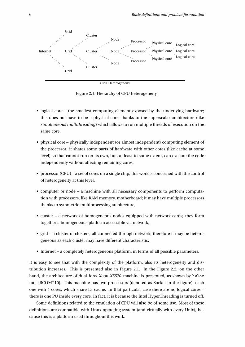
Figure 2.1: Hierarchy of CPU heterogeneity.
• logical core – the smallest computing element exposed by the underlying hardware;
this does not have to be a physical core, thanks to the superscalar architecture (like
simultaneous multithreading) which allows to run multiple threads of execution on the
same core,
• physical core – physically independent (or almost independent) computing element of
the processor; it shares some parts of hardware with other cores (like cache at some
level) so that cannot run on its own, but, at least to some extent, can execute the code
independently without affecting remaining cores,
• processor (CPU) – a set of cores on a single chip; this work is concerned with the control
of heterogeneity at this level,
• computer or node – a machine with all necessary components to perform computa-
tion with processors, like RAM memory, motherboard; it may have multiple processors
thanks to symmetric multiprocessing architecture,
• cluster – a network of homogeneous nodes equipped with network cards; they form
together a homogeneous platform accessible via network,
• grid – a cluster of clusters, all connected through network; therefore it may be hetero-
geneous as each cluster may have different characteristic,
• Internet – a completely heterogeneous platform, in terms of all possible parameters.
It is easy to see that with the complexity of the platform, also its heterogeneity and dis-
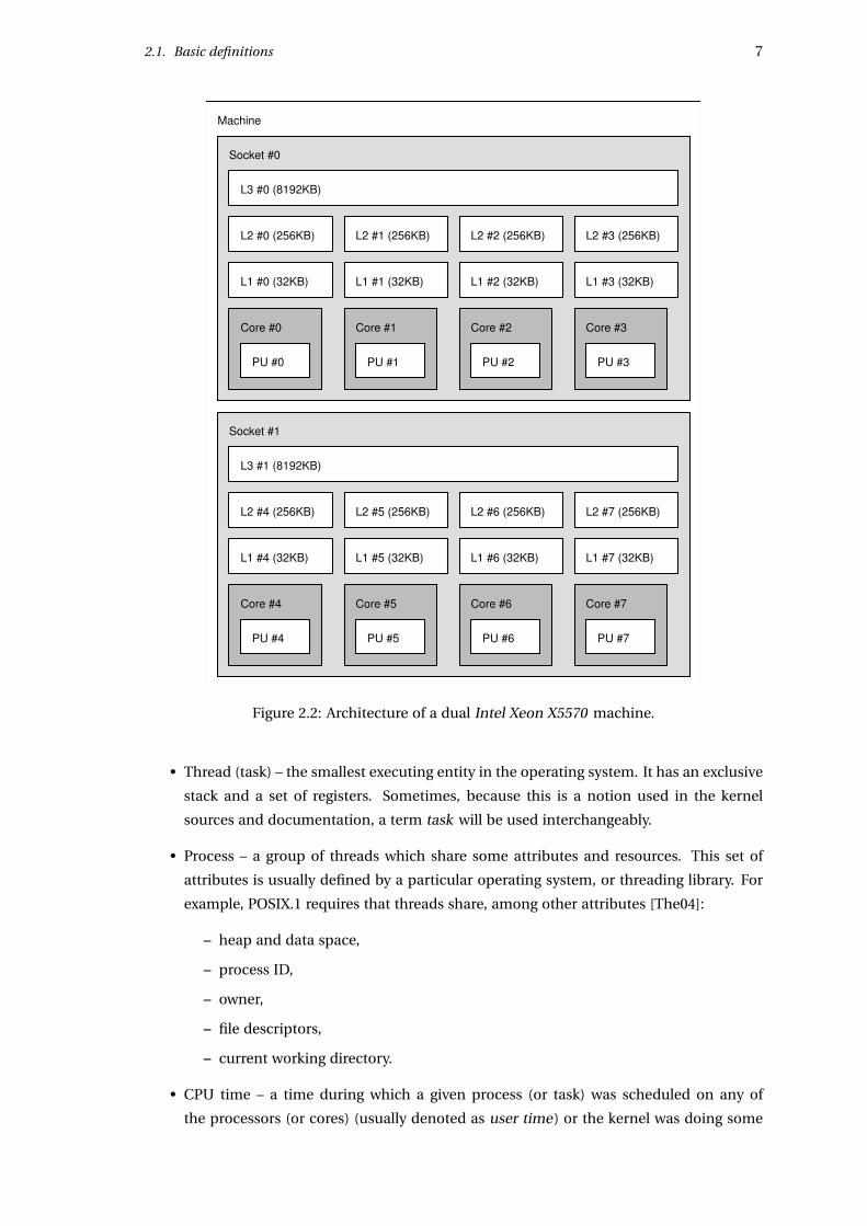
tribution increases. This is presented also in Figure 2.1. In the Figure 2.2, on the other
hand, the architecture of dual Intel Xeon X5570 machine is presented, as shown by hwloc
tool [BCOM+10]. This machine has two processors (denoted as Socket in the figure), each
one with 4 cores, which share L3 cache. In that particular case there are no logical cores –
there is one PU inside every core. In fact, it is because the Intel HyperThreading is turned off.
Some definitions related to the emulation of CPU will also be of some use. Most of these
definitions are compatible with Linux operating system (and virtually with every Unix), be-
cause this is a platform used throughout this work.
2.1. Basic definitions 7
Machine
Socket #0
L3 #0 (8192KB)
L2 #0 (256KB)
L1 #0 (32KB)
Core #0
PU #0
L2 #1 (256KB)
L1 #1 (32KB)
Core #1
PU #1
L2 #2 (256KB)
L1 #2 (32KB)
Core #2
PU #2
L2 #3 (256KB)
L1 #3 (32KB)
Core #3
PU #3
Socket #1
L3 #1 (8192KB)
L2 #4 (256KB)
L1 #4 (32KB)
Core #4
PU #4
L2 #5 (256KB)
L1 #5 (32KB)
Core #5
PU #5
L2 #6 (256KB)
L1 #6 (32KB)
Core #6
PU #6
L2 #7 (256KB)
L1 #7 (32KB)
Core #7
PU #7
Figure 2.2: Architecture of a dual Intel Xeon X5570 machine.
• Thread (task) – the smallest executing entity in the operating system. It has an exclusive
stack and a set of registers. Sometimes, because this is a notion used in the kernel
sources and documentation, a term task will be used interchangeably.
• Process – a group of threads which share some attributes and resources. This set of
attributes is usually defined by a particular operating system, or threading library. For
example, POSIX.1 requires that threads share, among other attributes [The04]:
– heap and data space,
– process ID,
– owner,
– file descriptors,
– current working directory.
• CPU time – a time during which a given process (or task) was scheduled on any of
the processors (or cores) (usually denoted as user time) or the kernel was doing some
8 Basic definitions and problem formulation
CPU work on the behalf of it (system time). This resonates with the definition used by
some Unix utilities (like time), or inside the Linux kernel itself. It always monotonously
increases, but does not have to be the same as the real time. In fact, it is always less
or equal to the real time, at least in the case of a single task process. Actually, when a
CPU-intensive, multithreaded process is executed on multi-core machine, its CPU time
may pass by faster than its real time! This is due to the fact that every thread may run
concurrently, executing multiple times more CPU cycles in the same period of time.
The difference between process CPU time and thread CPU time must be stressed here.
Usually the CPU time of a process is understood as a sum of all CPU times of its threads.
This is true for the above example, and will be true in this work.
• average CPU usage of a process/thread – a ratio of a process CPU time divided by the
period of time when this CPU time was measured:
average CPU usage = CPU time of the process/thread during the period
the period of time(2.1)
The definition of instant CPU usage, resembling a velocity (v(t )) defined as a derivative
of a distance (s(t ))
v(t ) = lim∆t→0
s(t +∆t )
∆t= s′(t )
is of no use here. CPU usage is not a continuous function, of course, and this kind of
limit does not exist. Anyway, it is possible to sample the timers in a very short intervals,
and computing this ratio as approximation to this limit. One must be aware that too
frequent requests of this information may largely influence that information, as retriev-
ing this information consumes some CPU power also. In some extreme cases this may
render the information completely useless, as in fact will be the case with CPU-Lim
method described in Section 3.2.2.
The important case of the average CPU usage, denoted simply as CPU usage will be the
following ratio:
CPU usage = total CPU time of the process/thread
lifetime of the process/thread(2.2)
• node – a computer node that is going to host emulated environments. As only proces-
sor parameters will be concerned, it can be characterized by a maximum frequency of
each core ( fmax ) (which is a common parameter for all of them) and a number of cores
available (N ): (fmax , N
)(2.3)
For example, the node already presented in Figure 2.2 may be represented by
(2.93 GHz,8). It is important to note that, although the emulation of heterogeneous
CPU architectures is interesting on its own, this work does not cover emulation of sys-
tems with such CPU configurations. It means that whenever a node with multiple cores
is given, then all of them have the same maximum frequency. This is hardly a limita-
tion, because virtually all existing systems are of this type. This also makes the whole
definition of node correct, as fmax is well-defined now.
2.2. Formulation of the problem 9
0 1 2 3
Virtual node
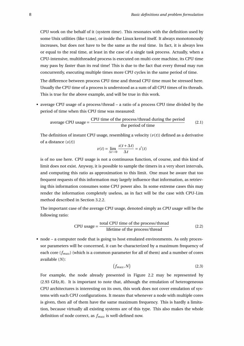
Figure 2.3: A visual representation of a virtual node(0.3,
{0,2,3
})based on a node with
fmax = 3 GHz.
• emulated frequency – a frequency f of processor that is going to be emulated by means
of methods presented later. It may sound somehow cloudy for the time being, but will
be defined more precisely in problem formulation in Section 2.2.
• emulation ratio – a ratio of emulated frequency ( f ) and maximum frequency of the
CPU ( fmax ):
µ= f
fmax(2.4)
• virtual node – a subset of processor’s cores that forms an independent scheduling group
of processes with a defined emulation ratio. Therefore, it may be represented by a pair(µ,C
)(2.5)
where µ is, as before, emulation ratio, and C is a subset of cores of a given processor.
The convention will be to identify cores with their numbering exported by the Linux
kernel, i.e., the integer identifiers of logical cores starting from 0, up to N −1 where N
is a number of cores of the processor.
For example, to describe a virtual node V N spanning 3 cores (say, cores 0, 2 and 3) of 4
core machine whose emulation ratio is µ= 0.3, one can write:
V N = (0.3,
{0,2,3
})This is presented in Figure 2.3. When the maximum frequency of a given node is known,
it is easy to calculate emulation frequency f using emulation ratio µ, and vice versa, by
means of Equation 2.4 only. For example, for the case in Figure 2.3, where fmax = 3 GHz,
one can compute
f =µ · fmax = 0.3 ·3 GHz = 900 MHz
2.2 Formulation of the problem
This work aims for a precise and robust solution for multi-core processor emulation problem,
i.e., to achieve the following goals:
1. Emulation of a different processor frequency than the one given by the manufacturer
of the hardware. The results obtained that way should be reproducible and mimic the
10 Basic definitions and problem formulation
0 1 2 3 4 5 6 7
VN 1 VN 2 VN 3 Virtual node 4
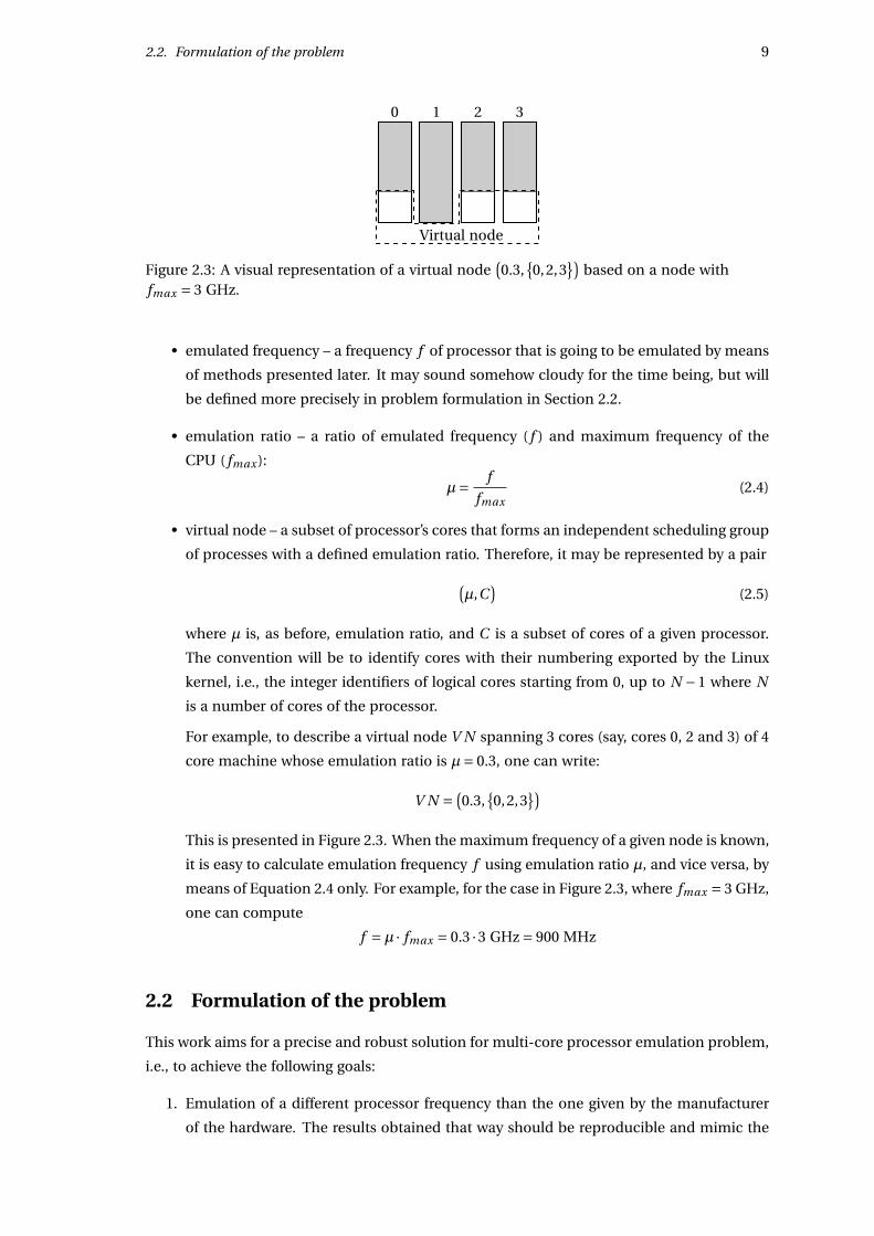
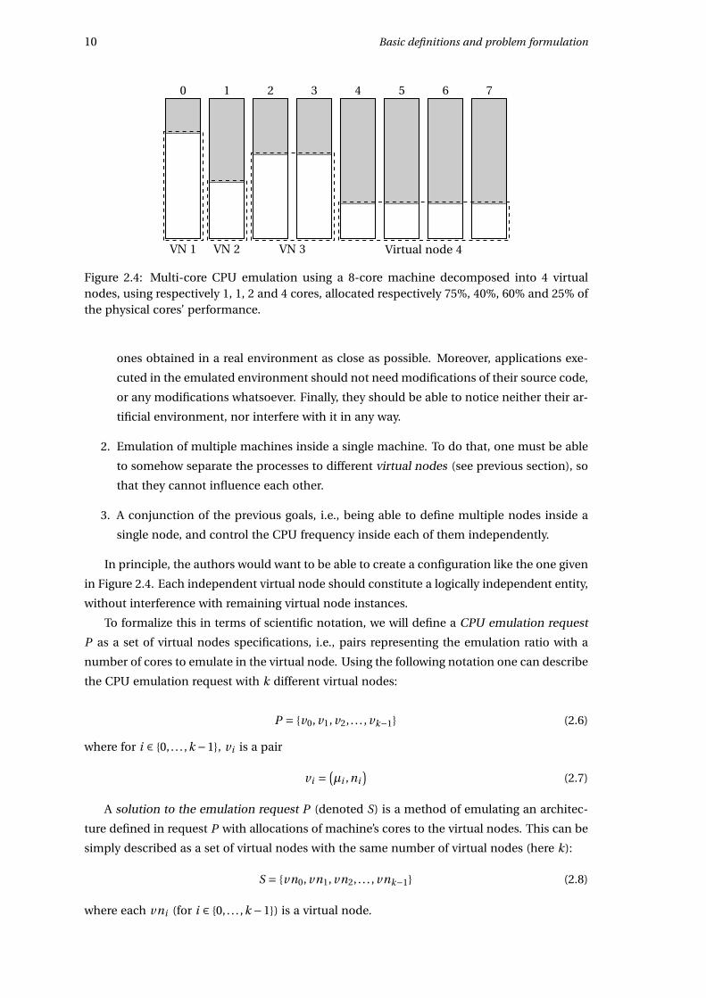
Figure 2.4: Multi-core CPU emulation using a 8-core machine decomposed into 4 virtualnodes, using respectively 1, 1, 2 and 4 cores, allocated respectively 75%, 40%, 60% and 25% ofthe physical cores’ performance.
ones obtained in a real environment as close as possible. Moreover, applications exe-
cuted in the emulated environment should not need modifications of their source code,
or any modifications whatsoever. Finally, they should be able to notice neither their ar-
tificial environment, nor interfere with it in any way.
2. Emulation of multiple machines inside a single machine. To do that, one must be able
to somehow separate the processes to different virtual nodes (see previous section), so
that they cannot influence each other.
3. A conjunction of the previous goals, i.e., being able to define multiple nodes inside a
single node, and control the CPU frequency inside each of them independently.
In principle, the authors would want to be able to create a configuration like the one given
in Figure 2.4. Each independent virtual node should constitute a logically independent entity,
without interference with remaining virtual node instances.
To formalize this in terms of scientific notation, we will define a CPU emulation request
P as a set of virtual nodes specifications, i.e., pairs representing the emulation ratio with a
number of cores to emulate in the virtual node. Using the following notation one can describe
the CPU emulation request with k different virtual nodes:
P = {v0, v1, v2, . . . , vk−1} (2.6)
where for i ∈ {0, . . . ,k −1}, vi is a pair
vi =(µi ,ni
)(2.7)
A solution to the emulation request P (denoted S) is a method of emulating an architec-
ture defined in request P with allocations of machine’s cores to the virtual nodes. This can be
simply described as a set of virtual nodes with the same number of virtual nodes (here k):
S = {vn0, vn1, vn2, . . . , vnk−1} (2.8)
where each vni (for i ∈ {0, . . . ,k −1}) is a virtual node.
2.2. Formulation of the problem 11
For example, the situation in Figure 2.4 can be represented by:{(0.75,1) , (0.6,2) , (0.4,1) , (0.25,4)
}and solved by means of some emulation method (which here is assumed to be known) and
the following allocations:{(0.75,{0}) , (0.4, {1}) , (0.6, {2,3}) , (0.25,{4,5,6,7})
}Basically, what happens here is that the request for a number of cores is replaced by the
allocations to logical cores of the machine. Notice also, that the ordering of elements in P
and S is unimportant because they are sets. Moreover, in general the allocation of CPU cores
is not unique. Some methods may put some restrictions on that, however, as we will see.
Not every request can be satisfied, of course. Generally, it depends on:
1. CPU emulation ratio µ – it must be a positive number less equal or less than 1.
2. Number of processors in the system – the number of cores in the request must be equal
or smaller than the number of physical cores. Moreover, one core must be assigned
exclusively to one virtual node.
3. CPU architecture of the system – some approaches have to take the advanced configu-
ration of processors into the account (e.g. CPU-Freq and CPU-Gov).
Ideally, a valid method solving the CPU emulation problem associated with the request P
must possess the following properties:
1. Correctness – the partition to virtual nodes and their emulated speed must be respected
under any kind of the emulated work.
2. Accuracy – the speed of a processor perceived by emulated tasks must agree with the re-
quest precisely. It means that the execution speed for CPU-bound tasks is proportional
to the emulation ratio µ.
3. Stability – repeated executions of the same emulation request should always yield re-
sults close to each other. In other words, the emulation environment should be deter-
ministic and reproducible.
4. Scalability – the emulation method should work properly no matter how many tasks
are emulated. Methods that add only a constant overhead are preferable to ones that,
for example, add a constant overhead for each emulated task.
5. No intrusiveness – the emulation must work "out-of-the-box", i.e., no significant changes
to the emulated software and operating system need to be done. Also the emulation
must not interfere with a normal execution of programs.
6. Portability – the method should be portable to other operating systems, if possible.
Any method that strives to fulfill these conditions and consequently to emulate the architec-
ture described by the CPU emulation request P , is a potential solution to the CPU emulation
problem.
12 Basic definitions and problem formulation
2.3 Complexity of the problem
The problem of CPU emulation in multi-core systems is closely related to scheduling. A clev-
erly written scheduler could be an elegant way to emulate CPUs at different speeds. Later, it
will be also shown that some presented methods here are actually doing a kind of work usu-
ally attributed to the scheduler, or are fundamentally using some features of the scheduler of
the operating system. As scheduling problems are in general tremendously complicated, we
postulate that CPU emulation is, at least to some degree, also a complicated problem.
In the previous section, the most informal part of the definition of the solution to CPU
emulation problem was the emulation method. It seems that, to some extent, the CPU emu-
lation problem is a wicked problem [RW73]. The wicked problem can be defined descriptively
using the following conditions (they differ slightly from the original setting, but still carry the
main meaning):
1. You do not understand the problem until you have developed a solution.
2. Wicked problems have no stopping rule.
3. Solutions to wicked problems are neither right nor wrong. They are simply better or
worse.
4. Every wicked problem is essentially unique and novel.
5. Every solution to a wicked problem is a "one-shot operation".
6. Wicked problems have no given alternative solutions.
The first condition is true for the defined problem. Of course there is a general idea what
the problem is, i.e., what the multi-core CPU emulation consists in, but what are the precise,
formal requirements is not obvious at all. Gradually, it should be more and more clear what
the good method is, with quantitative results obtained in Chapter 5. For now, the reader must
rely on the high-level requirement given in the previous section - the method must create an
environment with a different perceived CPU performance, which imitates the real one with
the same CPU configuration.
Sadly, the second condition applies here as well. Even if the best method is tested under
numerous hypotheses, one cannot be completely sure that it will stand for the next experi-
ment. Possibly, under different conditions the method will perform poorly. Surprisingly, that
was the case for methods for CPU emulation presented in this work - after encouraging re-
sults obtained using some of them, their usefulness had to be refuted, after successive exper-
iments. One way to circumvent this problem is to agree at some point that the solution "is
good enough".
The truthfulness of the next condition will be observed in Chapter 5. It will be plain that
no method is perfect in all tested cases. Some of them perform exceedingly better in most of
the cases, yet in other scenarios may be far from perfect.
The fourth condition concerning novelty of the problem will be discussed in the next sec-
tion, and will clearly show that this problem was not considered yet, at least at such level of
generality.
2.4. Related work and the current state of knowledge 13
The penultimate condition states only that the solutions given are applicable in the lim-
ited sense. This will be true, unfortunately, as we will see that some methods depend on a
very specific features available only in some operating systems (in this case - Linux) or even
in concrete releases of them. This greatly limits the portability of solutions and shows that
the work may have to be redone if the previous solution no longer solves the problem.
One has to agree also with the last condition. It means that there may be no final solutions
to the CPU emulation problem, or there may be other approaches, still unexplored. At the
very end it is a matter of creativity to devise new approaches, and a matter of taste to judge
them, to decide which ones to pursue and exercise. There is definitely no obvious way to
explore that subject completely rigorously.
2.4 Related work and the current state of knowledge
Several technologies and techniques enable the execution of applications under a different
perceived or real CPU speed.
Dynamic frequency scaling (known as Intel SpeedStep, AMD PowerNow! on laptops, and
AMD Cool’n’Quiet on desktops and servers) is a hardware technique to adjust the frequency
of CPUs, mainly for power-saving purposes. The frequency may be changed automatically by
the operating system according to the current system load, or set manually by the user. For
example, Linux exposes a frequency scaling interface using its sysfs pseudo-filesystem, and
provides several governors that react differently to changes of system load. In most CPUs,
those technologies only provide a few frequency levels (in the order of 5), but some CPUs
provide a lot more (11 levels on Xeon X5570, ranging from 1.6 GHz to 2.93 GHz). Moreover,
the transition time between different frequency levels is non-zero, and as will be noted later
(Section 3.3.3) this will impose some restrictions and the applicability of this method.
CPU-Lim is a CPU limiter implemented in Wrekavoc [CDGJ10]. It is implemented com-
pletely in user-space, using a real-time process that monitors the CPU usage of programs
executed by a predefined user. If a program has too big share of CPU time, it is stopped using
the SIGSTOP signal. If, after some time, this share falls below the specified threshold, then the
process is resumed using the SIGCONT signal. The measure of CPU load of a given process
is approximated by CPU usage defined previously.
CPU-Lim has the advantages of being simple and portable to most POSIX systems. How-
ever, it has several drawbacks, described in much detail in Section 3.2.2.
KRASH [PH10] is a CPU load injection tool. It is capable of recording and generating
reproducible system load on computing nodes. It is not a CPU speed degradation method
per se, but similar ideas have been used to design one of the methods presented later in this
paper, i.e., Fracas.
Using special features and properties of the Linux kernel to manage groups of processes,
a CPU-bound process is created on every CPU core and assigned a desired portion of CPU
time by setting its available CPU share.
Although there are many virtualization technologies available, due to their focus on per-
formance none of them offer any way to emulate lower CPU speed: they only allow to restrict
14 Basic definitions and problem formulation
a virtual machine to a subset of CPU cores, which is not sufficient for our purposes. It is also
possible to take an opposite approach, and modify the virtual machine hypervisor to change
its perception of time (time dilation), giving it the impression that the underlying hardware
runs faster or slower [GVV08].
Another approach is to emulate the whole computer architecture using the virtualization
technology, which is becoming more and more popular. The available virtualization products
(VirtualBox, VMWare products, Virtual PC) do not posses the ability to control the speed of
CPU inside the virtual machine. Actually, at least in the case of VirtualBox, they mimic the
physical processor of the host system, giving the guest operating system an impression that it
is available exclusively to it. Still, virtualization technology may be too artificial environment
as to yield results resonating with the real life experiments.
Bochs Emulator [BOC], which can be configured to perform a specific number of "em-
ulating instructions per second". However, according to Bochs’s documentation, that mea-
sure depends on the hosting operating system, the compiler configuration and the processor
speed. As Bochs is a fully emulated environment, this approach introduces performance im-
pact that is too high for our needs. Therefore, it is not covered in this work.
As a final remark, let us recall that CPU degradation can also be used used to run old
games on modern computers. Some ill-designed games, sensitive to the speed of the execu-
tion, are running simply too fast on current hardware and the player is unable to play. Burn-
ing of CPU cycles (which can be thought as a naive method of CPU emulation) is a common
way to solve (or rather work-around) that problem.
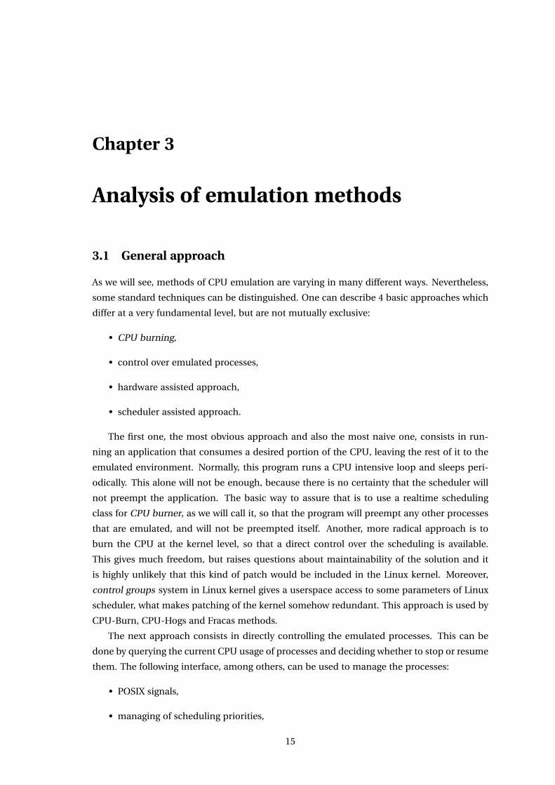
Chapter 3
Analysis of emulation methods
3.1 General approach
As we will see, methods of CPU emulation are varying in many different ways. Nevertheless,
some standard techniques can be distinguished. One can describe 4 basic approaches which
differ at a very fundamental level, but are not mutually exclusive:
• CPU burning,
• control over emulated processes,
• hardware assisted approach,
• scheduler assisted approach.
The first one, the most obvious approach and also the most naive one, consists in run-
ning an application that consumes a desired portion of the CPU, leaving the rest of it to the
emulated environment. Normally, this program runs a CPU intensive loop and sleeps peri-
odically. This alone will not be enough, because there is no certainty that the scheduler will
not preempt the application. The basic way to assure that is to use a realtime scheduling
class for CPU burner, as we will call it, so that the program will preempt any other processes
that are emulated, and will not be preempted itself. Another, more radical approach is to
burn the CPU at the kernel level, so that a direct control over the scheduling is available.
This gives much freedom, but raises questions about maintainability of the solution and it
is highly unlikely that this kind of patch would be included in the Linux kernel. Moreover,
control groups system in Linux kernel gives a userspace access to some parameters of Linux
scheduler, what makes patching of the kernel somehow redundant. This approach is used by
CPU-Burn, CPU-Hogs and Fracas methods.
The next approach consists in directly controlling the emulated processes. This can be
done by querying the current CPU usage of processes and deciding whether to stop or resume
them. The following interface, among others, can be used to manage the processes:
• POSIX signals,
• managing of scheduling priorities,
15
16 Analysis of emulation methods
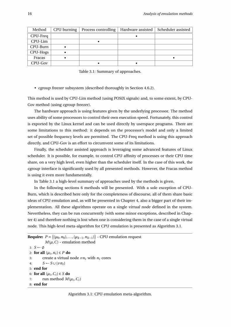
Method CPU burning Process controlling Hardware assisted Scheduler assisted
CPU-Freq •CPU-Lim •
CPU-Burn •CPU-Hogs •
Fracas • •CPU-Gov • •
Table 3.1: Summary of approaches.
• cgroup freezer subsystem (described thoroughly in Section 4.6.2).
This method is used by CPU-Lim method (using POSIX signals) and, to some extent, by CPU-
Gov method (using cgroup freezer).
The hardware approach is using features given by the underlying processor. The method
uses ability of some processors to control their own execution speed. Fortunately, this control
is exported by the Linux kernel and can be used directly by userspace programs. There are
some limitations to this method: it depends on the processor’s model and only a limited
set of possible frequency levels are permitted. The CPU-Freq method is using this approach
directly, and CPU-Gov is an effort to circumvent some of its limitations.
Finally, the scheduler assisted approach is leveraging some advanced features of Linux
scheduler. It is possible, for example, to control CPU affinity of processes or their CPU time
share, on a very high level, even higher than the scheduler itself. In the case of this work, the
cgroup interface is significantly used by all presented methods. However, the Fracas method
is using it even more fundamentally.
In Table 3.1 a high-level summary of approaches used by the methods is given.
In the following sections 6 methods will be presented. With a sole exception of CPU-
Burn, which is described here only for the completeness of discourse, all of them share basic
ideas of CPU emulation and, as will be presented in Chapter 4, also a bigger part of their im-
plementation. All these algorithms operate on a single virtual node defined in the system.
Nevertheless, they can be run concurrently (with some minor exceptions, described in Chap-
ter 4) and therefore nothing is lost when one is considering them in the case of a single virtual
node. This high-level meta-algorithm for CPU emulation is presented as Algorithm 3.1.
Require: P = {(µ0,n0), . . . , (µk−1,nk−1)
}- CPU emulation request
Require: M(µ,C ) - emulation method1: S ←;2: for all (µi ,ni ) ∈ P do3: create a virtual node vni with ni cores4: S ← S ∪ {vni }5: end for6: for all (µi ,Ci ) ∈ S do7: run method M(µi ,Ci )8: end for
Algorithm 3.1: CPU emulation meta-algorithm.
3.2. Existing methods 17
The abstract method M(µ,C ) in this algorithm is parametrized by two parameters: the
emulation ratio (µ) and a subset of cores where the emulation must be performed (C ). In
some methods additional parameters may be needed, but that was omitted for the sake of
brevity.
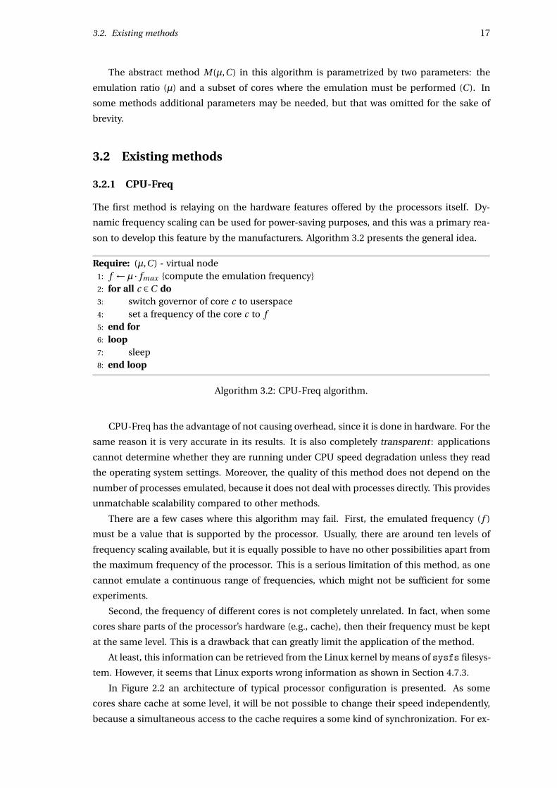
3.2 Existing methods
3.2.1 CPU-Freq
The first method is relaying on the hardware features offered by the processors itself. Dy-
namic frequency scaling can be used for power-saving purposes, and this was a primary rea-
son to develop this feature by the manufacturers. Algorithm 3.2 presents the general idea.
Require: (µ,C ) - virtual node1: f ←µ · fmax {compute the emulation frequency}2: for all c ∈C do3: switch governor of core c to userspace4: set a frequency of the core c to f5: end for6: loop7: sleep8: end loop
Algorithm 3.2: CPU-Freq algorithm.
CPU-Freq has the advantage of not causing overhead, since it is done in hardware. For the
same reason it is very accurate in its results. It is also completely transparent : applications
cannot determine whether they are running under CPU speed degradation unless they read
the operating system settings. Moreover, the quality of this method does not depend on the
number of processes emulated, because it does not deal with processes directly. This provides
unmatchable scalability compared to other methods.
There are a few cases where this algorithm may fail. First, the emulated frequency ( f )
must be a value that is supported by the processor. Usually, there are around ten levels of
frequency scaling available, but it is equally possible to have no other possibilities apart from
the maximum frequency of the processor. This is a serious limitation of this method, as one
cannot emulate a continuous range of frequencies, which might not be sufficient for some
experiments.
Second, the frequency of different cores is not completely unrelated. In fact, when some
cores share parts of the processor’s hardware (e.g., cache), then their frequency must be kept
at the same level. This is a drawback that can greatly limit the application of the method.
At least, this information can be retrieved from the Linux kernel by means of sysfs filesys-
tem. However, it seems that Linux exports wrong information as shown in Section 4.7.3.
In Figure 2.2 an architecture of typical processor configuration is presented. As some
cores share cache at some level, it will be not possible to change their speed independently,
because a simultaneous access to the cache requires a some kind of synchronization. For ex-
18 Analysis of emulation methods
ample, the cores identified by numbers 0 and 3 must run at the same speed, because they
share L3 cache.
Another disadvantage is that this method relies on the frequencies advertised by the CPU.
On some AMD CPUs, some advertised frequencies were experimentally determined to be
rounded values of the real frequency (the performance was not growing linearly with the fre-
quency). It would be possible to work-around this issue by adding a calibration phase where
the performance offered by each advertised frequency would be measured.
Advantages:
• very high accuracy,
• no additional overhead when set up,
• transparent,
• scalable with number of processes.
Disadvantages:
• limited to the available frequency levels,
• applicability depends on the internal architecture of the processor,
• may be biased by hardware implementation.
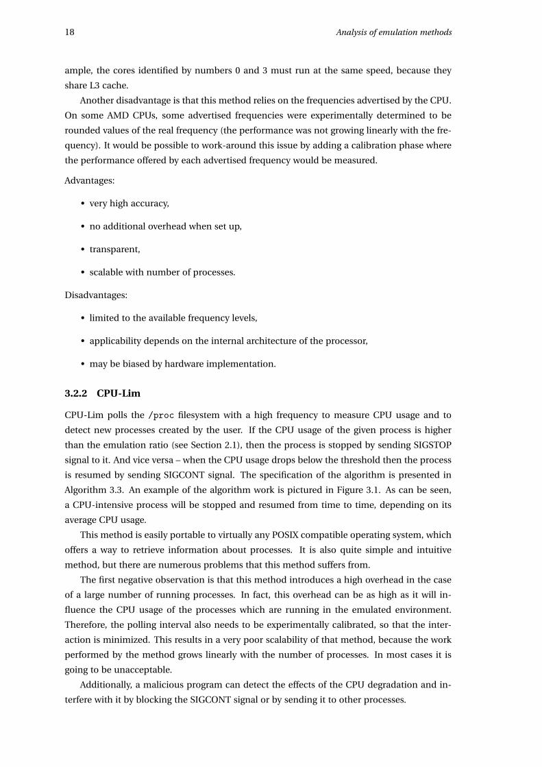
3.2.2 CPU-Lim
CPU-Lim polls the /proc filesystem with a high frequency to measure CPU usage and to
detect new processes created by the user. If the CPU usage of the given process is higher
than the emulation ratio (see Section 2.1), then the process is stopped by sending SIGSTOP
signal to it. And vice versa – when the CPU usage drops below the threshold then the process
is resumed by sending SIGCONT signal. The specification of the algorithm is presented in
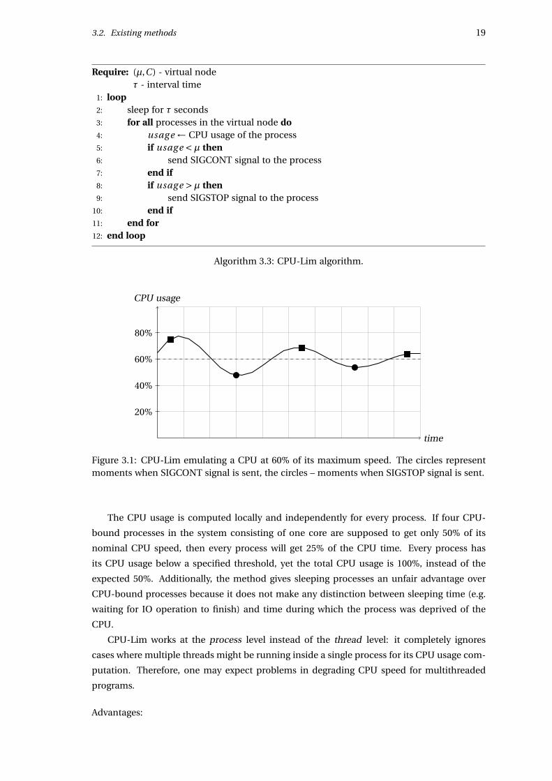
Algorithm 3.3. An example of the algorithm work is pictured in Figure 3.1. As can be seen,
a CPU-intensive process will be stopped and resumed from time to time, depending on its
average CPU usage.
This method is easily portable to virtually any POSIX compatible operating system, which
offers a way to retrieve information about processes. It is also quite simple and intuitive
method, but there are numerous problems that this method suffers from.
The first negative observation is that this method introduces a high overhead in the case
of a large number of running processes. In fact, this overhead can be as high as it will in-
fluence the CPU usage of the processes which are running in the emulated environment.
Therefore, the polling interval also needs to be experimentally calibrated, so that the inter-
action is minimized. This results in a very poor scalability of that method, because the work
performed by the method grows linearly with the number of processes. In most cases it is
going to be unacceptable.
Additionally, a malicious program can detect the effects of the CPU degradation and in-
terfere with it by blocking the SIGCONT signal or by sending it to other processes.
3.2. Existing methods 19
Require: (µ,C ) - virtual nodeRequire: τ - interval time
1: loop2: sleep for τ seconds3: for all processes in the virtual node do4: usag e ← CPU usage of the process5: if usag e <µ then6: send SIGCONT signal to the process7: end if8: if usag e >µ then9: send SIGSTOP signal to the process
10: end if11: end for12: end loop
Algorithm 3.3: CPU-Lim algorithm.
time
CPU usage
20%
40%
60%
80%
Figure 3.1: CPU-Lim emulating a CPU at 60% of its maximum speed. The circles representmoments when SIGCONT signal is sent, the circles – moments when SIGSTOP signal is sent.
The CPU usage is computed locally and independently for every process. If four CPU-
bound processes in the system consisting of one core are supposed to get only 50% of its
nominal CPU speed, then every process will get 25% of the CPU time. Every process has
its CPU usage below a specified threshold, yet the total CPU usage is 100%, instead of the
expected 50%. Additionally, the method gives sleeping processes an unfair advantage over
CPU-bound processes because it does not make any distinction between sleeping time (e.g.
waiting for IO operation to finish) and time during which the process was deprived of the
CPU.
CPU-Lim works at the process level instead of the thread level: it completely ignores
cases where multiple threads might be running inside a single process for its CPU usage com-
putation. Therefore, one may expect problems in degrading CPU speed for multithreaded
programs.
Advantages:
20 Analysis of emulation methods
• simple and intuitive (incorrectly),
• portable.
Disadvantages:
• computational complexity of the method (linear with number of emulated processes),
• interference with normal work,
• problems with CPU usage measure,
• problems with multithreaded processes,
• required calibration of interval time.
3.2.3 CPU-Burn
A basic method to degrade the perceived CPU performance is to create a spinning process
that will use the CPU for the desired amount of time, before releasing it for the application.
This was already implemented in Wrekavoc [CDGJ10] as CPU-Burn method. One CPU burner
thread per core is created, and assigned to a specific core using scheduler affinity. They are
assigned the maximum realtime priority, so that they are always prioritized over other tasks
by the kernel. The CPU burners then alternatively spin and sleep for configurable amounts
of time (τ), leaving space for the other applications during the requested time intervals. The
high-level algorithm is presented in Algorithm 3.4.
Require: (µ,C ) - virtual nodeRequire: τ - interval time
1: for all c ∈C do2: create a CPU burning thread t (µ,τ)3: set the scheduling priority of t to realtime4: set the CPU affinity of t to the core c only5: end for6: loop7: sleep8: end loop
Algorithm 3.4: CPU-Burn algorithm.
It remains to describe how each CPU burner thread works. It is easy to see, that the time
spent on CPU burning (T ) must be
T = 1−µµ
τ (3.1)
where µ is emulation ratio and τ is the sleeping interval. To prove that, notice that µ must
be equal to the ratio of CPU time available to the emulated processes (τ) and the time of the
whole cycle (i.e., τ+T ):τ
T +τ = τ1−µµ τ+τ
= µτ
(1−µ)τ+µτ =µ (3.2)
3.3. Proposed methods 21
Require: µ - emulation ratioRequire: τ - interval time
1: T ← 1−µµ τ
2: loop3: sleep for τ seconds4: do CPU intensive work for T seconds5: end loop
Algorithm 3.5: CPU-Burn algorithm (performed by each CPU burner).
which is indeed the case. The algorithm of CPU-Burn method is presented in Algorithm 3.5.
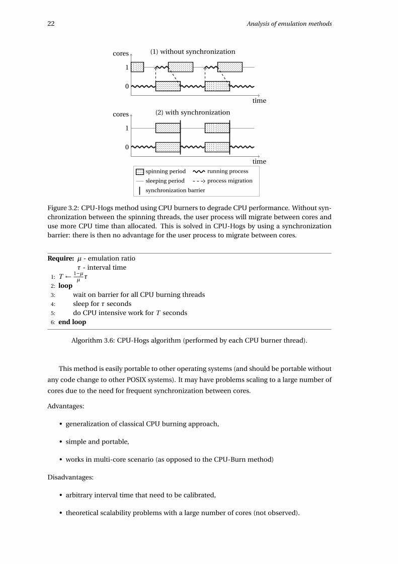
This method is very simple, but will not work for multi-core case properly. The CPU burn-
ing threads will desynchronize in a matter of seconds and the scheduler will migrate emulated
processes to other cores as is shown in Figure 3.2. The remedy for that is provided by the next
method described, i.e., CPU-Hogs, which can be thought as a spiritual successor of CPU-
Burn. The CPU-Burn method was described here only for the sake of completeness and will
not be considered later.
Advantages:
• generalization of classical CPU burning approach,
• simple and portable.
Disadvantages:
• does not work properly in multi-core case,
• arbitrary interval time that need to be calibrated.
3.3 Proposed methods
3.3.1 Cpu-Hogs
The CPU-Hogs method generalizes the idea of CPU burning to the multi-core case and fixes
problems associated with CPU-Burn method. They are almost identical, but the crucial
changes made in the very algorithm and reimplementation of the whole program were nec-
essary to achieve a properly working CPU emulation tool.
As previously mentioned, creating one CPU burner per core is not enough in the multi-
core case. If the spinning and sleeping periods are not synchronized between all cores, the
user processes will migrate between cores and benefit from more CPU time than expected
(Figure 3.2). This happens in practice due to interrupts or system calls processing that will
desynchronize the threads. In CPU-Hogs, the spinning threads are therefore synchronized
using a POSIX thread barrier placed at the beginning of each sleeping period. The high-level
algorithm remains the same as Algorithm 3.4 and the description of CPU burning threads is
given in Algorithm 3.6.
22 Analysis of emulation methods
cores
time
0
1
(1) without synchronization
cores
time
0
1
(2) with synchronization
spinning period
sleeping period
running process
process migration
synchronization barrier
Figure 3.2: CPU-Hogs method using CPU burners to degrade CPU performance. Without syn-chronization between the spinning threads, the user process will migrate between cores anduse more CPU time than allocated. This is solved in CPU-Hogs by using a synchronizationbarrier: there is then no advantage for the user process to migrate between cores.
Require: µ - emulation ratioRequire: τ - interval time
1: T ← 1−µµ τ
2: loop3: wait on barrier for all CPU burning threads4: sleep for τ seconds5: do CPU intensive work for T seconds6: end loop
Algorithm 3.6: CPU-Hogs algorithm (performed by each CPU burner thread).
This method is easily portable to other operating systems (and should be portable without
any code change to other POSIX systems). It may have problems scaling to a large number of
cores due to the need for frequent synchronization between cores.
Advantages:
• generalization of classical CPU burning approach,
• simple and portable,
• works in multi-core scenario (as opposed to the CPU-Burn method)
Disadvantages:
• arbitrary interval time that need to be calibrated,
• theoretical scalability problems with a large number of cores (not observed).
3.3. Proposed methods 23
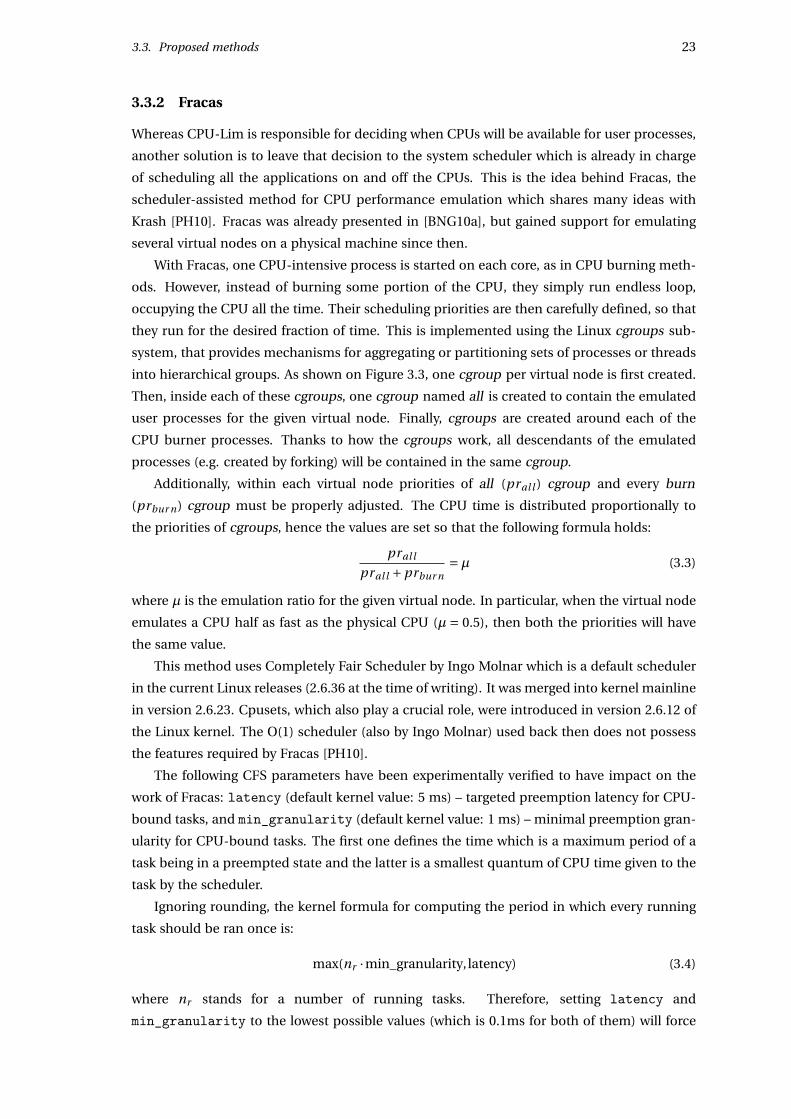
3.3.2 Fracas
Whereas CPU-Lim is responsible for deciding when CPUs will be available for user processes,
another solution is to leave that decision to the system scheduler which is already in charge
of scheduling all the applications on and off the CPUs. This is the idea behind Fracas, the
scheduler-assisted method for CPU performance emulation which shares many ideas with
Krash [PH10]. Fracas was already presented in [BNG10a], but gained support for emulating
several virtual nodes on a physical machine since then.
With Fracas, one CPU-intensive process is started on each core, as in CPU burning meth-
ods. However, instead of burning some portion of the CPU, they simply run endless loop,
occupying the CPU all the time. Their scheduling priorities are then carefully defined, so that
they run for the desired fraction of time. This is implemented using the Linux cgroups sub-
system, that provides mechanisms for aggregating or partitioning sets of processes or threads
into hierarchical groups. As shown on Figure 3.3, one cgroup per virtual node is first created.
Then, inside each of these cgroups, one cgroup named all is created to contain the emulated
user processes for the given virtual node. Finally, cgroups are created around each of the
CPU burner processes. Thanks to how the cgroups work, all descendants of the emulated
processes (e.g. created by forking) will be contained in the same cgroup.
Additionally, within each virtual node priorities of all (pral l ) cgroup and every burn
(prbur n) cgroup must be properly adjusted. The CPU time is distributed proportionally to
the priorities of cgroups, hence the values are set so that the following formula holds:
pral l
pral l +prbur n=µ (3.3)
where µ is the emulation ratio for the given virtual node. In particular, when the virtual node
emulates a CPU half as fast as the physical CPU (µ = 0.5), then both the priorities will have
the same value.
This method uses Completely Fair Scheduler by Ingo Molnar which is a default scheduler
in the current Linux releases (2.6.36 at the time of writing). It was merged into kernel mainline
in version 2.6.23. Cpusets, which also play a crucial role, were introduced in version 2.6.12 of
the Linux kernel. The O(1) scheduler (also by Ingo Molnar) used back then does not possess
the features required by Fracas [PH10].
The following CFS parameters have been experimentally verified to have impact on the
work of Fracas: latency (default kernel value: 5 ms) – targeted preemption latency for CPU-
bound tasks, and min_granularity (default kernel value: 1 ms) – minimal preemption gran-
ularity for CPU-bound tasks. The first one defines the time which is a maximum period of a
task being in a preempted state and the latter is a smallest quantum of CPU time given to the
task by the scheduler.
Ignoring rounding, the kernel formula for computing the period in which every running
task should be ran once is:
max(nr ·min_granularity, latency) (3.4)
where nr stands for a number of running tasks. Therefore, setting latency and
min_granularity to the lowest possible values (which is 0.1ms for both of them) will force
24 Analysis of emulation methods
root cgroup
vn1 vn2 vn3 vn4
all all all all
bur n0 bur n1 bur n2 bur n3 bur n4 bur n5 bur n6 bur n7
process without
emulation (sys-
tem daemons, etc)
CPU burneremulated process
Figure 3.3: Structure of cgroups in Fracas for the example from Figure 2.4. This also gives aglimpse of internal structure of virtual nodes for all methods (see Chapter 4).
the scheduler to compute the smallest possible preemption periods and, as a result, the high-
est possible activity of the scheduler. Because of these observations the Fracas method
changes the settings of the scheduler to improve the results.
To conclude the discussion, the algorithm used by the Fracas method is presented as Al-
gorithm 3.7.
Require: (µ,C ) - virtual node1: pral l ← 1 {arbitrary, positive constant}2: prbur n ← pral l
µ −pral l {see Equation 3.3}3: tune parameters of the scheduler4: create all cgroup in (µ,C ) with priority pral l
5: move all emulated processes to all6: for all c ∈C do7: create bur nc cgroup in (µ,C ) with priority prbur n
8: run CPU burner in bur nc
9: end for10: loop11: sleep12: end loop
Algorithm 3.7: Fracas algorithm.
It is worth noting that the implementation of Fracas is strongly related to the Linux ker-
nel’s internals: as the scheduling is offloaded to the kernel’s scheduler, subtle changes to the
system scheduler can severely affect the correctness of Fracas. Results presented in this paper
were obtained using Linux 2.6.33.2, but older kernel versions (for example, version 2.6.32.15)
exhibited a very different behavior.
This method relies on several recent Linux-specific features and interfaces and is not
3.3. Proposed methods 25
portable to different operating systems. However, it has several advantages. First, it is com-
pletely transparent, since it works at the kernel level. Processes cannot notice the injected
load directly, nor interfere with it. Second, this approach is very scalable with the number of
controlled processes: no polling is involved, and there are no parameters to calibrate.
Advantages:
• passive, i.e., requires no additional work when set up,
• transparent to the emulated processes,
• scalable.
Disadvantages:
• not portable,
• sensitive to the configuration of the scheduler,
• sensitive to subtle changes in the kernel.
3.3.3 CPU-Gov
Similarly to CPU-Freq method, CPU-Gov is a hardware-assisted approach. It may be consid-
ered a spiritual successor to CPU-Freq method, because it solves the main issue of CPU-Freq
method - the inability to emulate a continuous range of frequency values. Still, it inherits
some problems of its predecessor.
CPU-Gov leverages the hardware frequency scaling to provide emulation by switching be-
tween the two frequencies that are directly lower or equal ( fL) and higher or equal ( fH ) than
the requested emulated frequency ( f ). Precisely, when k frequency levels supported by the
kernel are f1 < f2 < . . . < fk and f falls between, say, fm and fm+1, then we have:
f1 < . . . < fm = fL ≤ f ≤ fH = fm+1 < . . . < fk
The time spent at the lower frequency (tL) and at the higher frequency (tH ) must satisfy the
following formula:
f = fL tL + fH tH
tL + tH(3.5)
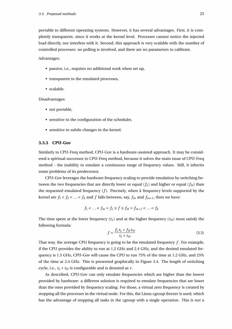
That way, the average CPU frequency is going to be the emulated frequency f . For example,
if the CPU provides the ability to run at 1.2 GHz and 2.4 GHz, and the desired emulated fre-
quency is 1.5 GHz, CPU-Gov will cause the CPU to run 75% of the time at 1.2 GHz, and 25%
of the time at 2.4 GHz. This is presented graphically in Figure 3.4. The length of switching
cycle, i.e., tL + tH is configurable and is denoted as τ.
As described, CPU-Gov can only emulate frequencies which are higher than the lowest
provided by hardware: a different solution is required to emulate frequencies that are lower
than the ones provided by frequency scaling. For those, a virtual zero frequency is created by
stopping all the processes in the virtual node. For this, the Linux cgroup freezer is used, which
has the advantage of stopping all tasks in the cgroup with a single operation. This is not a
26 Analysis of emulation methods
fL = 1.2 GHz f H=
2.4
GH
z
τ
f = 1.5 GHz
τ
tL = 0.75τ tH = 0.25τ
Figure 3.4: An illustration of CPU-Gov frequency switching. The sum of areas of two rectan-gles on the left are exactly the area of the rectangle on the right. That is, on the average CPUspeed is 1.5 GHz.
completely atomic operation and, as a matter of a fact, two bugs in the Linux kernel were
found when working on the CPU-Gov method (see Section 4.7.2). Although this is a clever
and working solution to this problem, it changes dramatically the behavior of the method in
that case.
After this discussion it can be assumed that there is always 0 GHz frequency level avail-
able. To keep things simple, the special case described above is not treated in a special way
in the following following Algorithm 3.8. The computations are actually carried exactly the
same way as before, but there is a virtual f0 = 0 GHz frequency level available. This makes the
CPU-Gov method applicable even if there is no hardware support for frequency scaling pro-
vided. In that case, only two different levels are available: zero frequency and the maximum
frequency of the CPU.
When either tL = 0 or tH = 0, then the method actually works similarly to CPU-Freq
method. It simply means that emulated frequency is exactly represented by one frequency
level of the hardware frequency scaling.
This method has the advantage that, when the frequency is higher than the lowest fre-
quency provided by hardware frequency scaling, the user application is constantly running
on the processor. Hence, its CPU time will be correct, what, with the exception of the CPU-
Freq method, is not the case for the other methods.
However, this method suffers from the limitation mentioned in Section 3.2.1 about fre-
quency scaling: on some CPUs, it is not possible to change the frequency of each core inde-
pendently. The related cores might have to be switched together for the change to take effect,
due to the sharing of caches, for example. This is taken into account when allocating vir-
tual nodes on cores, but limits the possible configurations. For example, on quad-core CPUs,
it might not be even possible to create 2 virtual nodes with different emulated frequencies.
Nevertheless, when different virtual nodes are assigned the same emulation frequency, then
the method is able to combine them into a one group and they can be switched together, as
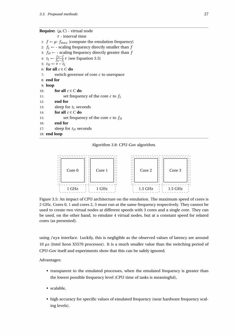
shown in Figure 3.5 .
Moreover, the transition between different frequency levels is not instant and some non-
zero time is needed for the processor to switch its circuits to a different operating frequency.
The information on that parameter of the processor can be retrieved from the Linux kernel
3.3. Proposed methods 27
Require: (µ,C ) - virtual nodeRequire: τ - interval time
1: f ←µ · fmax {compute the emulation frequency}2: fL ← - scaling frequency directly smaller than f3: fH ← - scaling frequency directly greater than f
4: tL ← fH− ffH− fL
τ {see Equation 3.5}5: tH ← τ− tL
6: for all c ∈C do7: switch governor of core c to userspace8: end for9: loop
10: for all c ∈C do11: set frequency of the core c to fL
12: end for13: sleep for tL seconds14: for all c ∈C do15: set frequency of the core c to fH
16: end for17: sleep for tH seconds18: end loop
Algorithm 3.8: CPU-Gov algorithm.
Core 0 Core 1
1 GHz 1 GHz
Core 2 Core 3
1.5 GHz 1.5 GHz
Figure 3.5: An impact of CPU architecture on the emulation. The maximum speed of cores is2 GHz. Cores 0, 1 and cores 2, 3 must run at the same frequency respectively. They cannot beused to create two virtual nodes at different speeds with 3 cores and a single core. They canbe used, on the other hand, to emulate 4 virtual nodes, but at a constant speed for relatedcores (as presented).
using /sys interface. Luckily, this is negligible as the observed values of latency are around
10 µs (Intel Xeon X5570 processor). It is a much smaller value than the switching period of
CPU-Gov itself and experiments show that this can be safely ignored.
Advantages:
• transparent to the emulated processes, when the emulated frequency is greater than
the lowest possible frequency level (CPU time of tasks is meaningful),
• scalable,
• high accuracy for specific values of emulated frequency (near hardware frequency scal-
ing levels).

28 Analysis of emulation methods
Disadvantages:
• applicability and accuracy of the method depends on the internal architecture of the
processor and the quality of hardware implementation,
• radically different behavior for small emulated frequencies.
Chapter 4
Design and implementation of
methods
4.1 Introduction
In the chapter to follow, important details of implementation are presented. By no means
this is going to be a complete description. Only important decisions, technical details and
problems encountered are to be presented.
To start with, the basic pieces of information concerning the work will be presented.
Then, the description of crucial parts of the project will be given, followed by a detailed dis-
course on the implementation of each method described in the previous chapter.
Finally, the problems met during the implementation will be presented, and the chapter
will be concluded with final remarks.
4.2 Organization of the work
The work on the project proceeded iteratively. First, the ideas how to emulate CPU perfor-
mance were devised and implemented. Some hypotheses about their behavior were postu-
lated, then experiments were carried out to validate them. This is a standard procedure in
the experimental science known as scientific method. This approach suggests also a devel-
opment model, which, with the properties of the CPU emulation problem (e.g., no precise
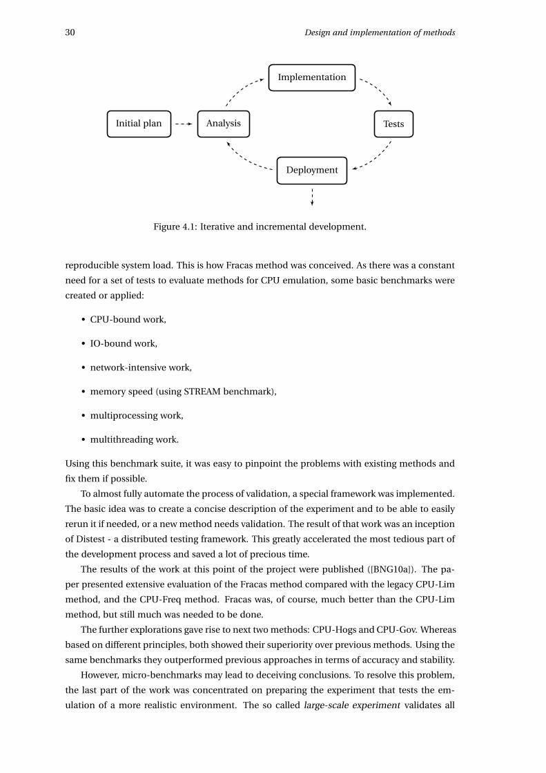
goals), already presented is Section 2.3, was chosen to be iterative and incremental.
Iterative and incremental development starts with the initial planning and finishes with
the deployment of the product. In between cyclic development cycles are carried out, each
consisting of analysis, implementation and testing phases [AJ97]. As the process is iterated, it
may not finish at deployment phase. Instead, a next iteration will be started to improve the
product.
The work started as a research on Wrekavoc tool [CDGJ10]. Soon, it was concluded that
CPU emulation part of this application lacks accuracy and robustness. The study of the
source code and basic experiments performed on methods implemented in it (CPU-Lim and
CPU-Burn) revealed that these methods lack robustness and accuracy.
The first idea was to use the idea presented in KRASH [PH10], which is a tool to generate
29
30 Design and implementation of methods
AnalysisInitial plan
Implementation
Deployment
Tests
Figure 4.1: Iterative and incremental development.
reproducible system load. This is how Fracas method was conceived. As there was a constant
need for a set of tests to evaluate methods for CPU emulation, some basic benchmarks were
created or applied:
• CPU-bound work,
• IO-bound work,
• network-intensive work,
• memory speed (using STREAM benchmark),
• multiprocessing work,
• multithreading work.
Using this benchmark suite, it was easy to pinpoint the problems with existing methods and
fix them if possible.
To almost fully automate the process of validation, a special framework was implemented.
The basic idea was to create a concise description of the experiment and to be able to easily
rerun it if needed, or a new method needs validation. The result of that work was an inception
of Distest - a distributed testing framework. This greatly accelerated the most tedious part of
the development process and saved a lot of precious time.
The results of the work at this point of the project were published ([BNG10a]). The pa-
per presented extensive evaluation of the Fracas method compared with the legacy CPU-Lim
method, and the CPU-Freq method. Fracas was, of course, much better than the CPU-Lim
method, but still much was needed to be done.
The further explorations gave rise to next two methods: CPU-Hogs and CPU-Gov. Whereas
based on different principles, both showed their superiority over previous methods. Using the
same benchmarks they outperformed previous approaches in terms of accuracy and stability.
However, micro-benchmarks may lead to deceiving conclusions. To resolve this problem,
the last part of the work was concentrated on preparing the experiment that tests the em-
ulation of a more realistic environment. The so called large-scale experiment validates all
4.3. Programming languages used 31
methods when used with a real application emulation, run on multiple nodes of homoge-
neous cluster.
As said before, the work consisted of numerous iterations. For example, the implementa-
tion of the method was tested, what led to discovery of some subtle bugs. After the necessary
fixes, the same method was evaluated again, and so on. When the method was sufficiently
stable for some time, it was kept frozen. The reason behind was the need of using one and
the only version of source code base for publications. This was sometimes problematic, as
the developers had to work with a version of software known to contain bugs. They had to
be bypassed by means of some "dirty" tricks, sometimes. For example, the CPU-Gov method,
which unveiled a bug in the Linux kernel contained a special piece of code, whose only task
was to make sure, that the bug will not be triggered.
The source code underwent a few major refactorizations over the time. The biggest one
extracted a large piece of redundant code from all CPU emulation methods. The shared code
base is now available as CPU emulation library (cpuemu) and is use extensively by almost
every program. Actually, some methods, like CPU-Freq, became very short and trivial in their
implementation, replacing previous, hand-crafted and unmaintainable implementations. Us-
ing the same library, some useful tools were written, which replaced long sequences of time-
consuming operations.
4.3 Programming languages used
Most of the source code is written in Python programming language. The version used was
Python 2.5 with some features sometimes backported from Python 2.6. For example, CPU
emulation library is written in Python, as all the CPU emulation methods frontends are.
Also a lot of C or C++ code was written for crucial parts of the methods or to access rou-
tines not available directly from high-level programming languages like Python. When some
kind of threading was necessary, POSIX threads library was used.
Finally, the description file of the experiment for Distest framework, even though being a
well-formed Python file, can be thought as a separate language. A more elaborate description
of the construction and the rules is given in Section 4.6.3.
4.4 Tools and libraries used
The research was done on the Linux operating system. The distribution used was Ubuntu 9.10
(Karmic Koala). Git was used as a revision control system. It offers a distributed approach
without a requirement of connection to the Internet. In Subversion revision control system,
for example, one cannot commit changes without Internet connection. This feature was very
important when the work happens to be done without access to the Internet, or this access is
restricted (by rigorous firewall policy, for example).
To synchronize the state of data at different hosts involved with the experiments, rsync
tool was used.
For some high-precision, scientific computations mpmath library [MPM] was used. It is
a library for Python implementing arithmetic operations of arbitrary high precision.
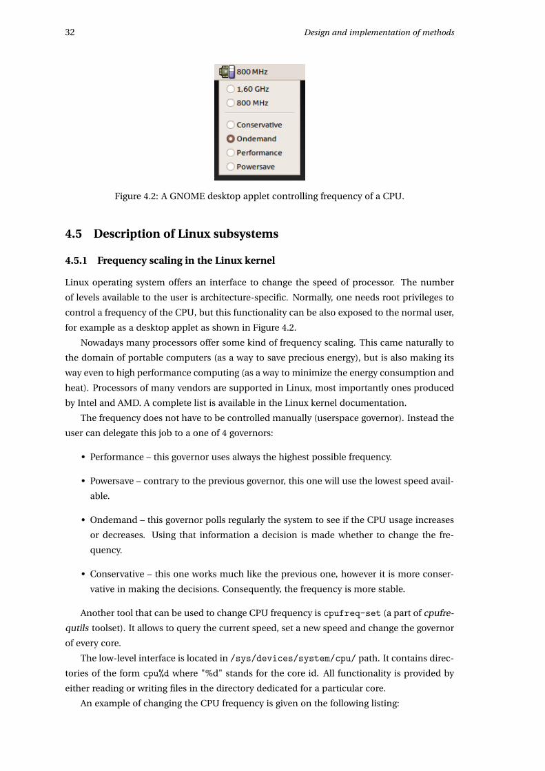
32 Design and implementation of methods
Figure 4.2: A GNOME desktop applet controlling frequency of a CPU.
4.5 Description of Linux subsystems
4.5.1 Frequency scaling in the Linux kernel
Linux operating system offers an interface to change the speed of processor. The number
of levels available to the user is architecture-specific. Normally, one needs root privileges to
control a frequency of the CPU, but this functionality can be also exposed to the normal user,
for example as a desktop applet as shown in Figure 4.2.
Nowadays many processors offer some kind of frequency scaling. This came naturally to
the domain of portable computers (as a way to save precious energy), but is also making its
way even to high performance computing (as a way to minimize the energy consumption and
heat). Processors of many vendors are supported in Linux, most importantly ones produced
by Intel and AMD. A complete list is available in the Linux kernel documentation.
The frequency does not have to be controlled manually (userspace governor). Instead the
user can delegate this job to a one of 4 governors:
• Performance – this governor uses always the highest possible frequency.
• Powersave – contrary to the previous governor, this one will use the lowest speed avail-
able.
• Ondemand – this governor polls regularly the system to see if the CPU usage increases
or decreases. Using that information a decision is made whether to change the fre-
quency.
• Conservative – this one works much like the previous one, however it is more conser-
vative in making the decisions. Consequently, the frequency is more stable.
Another tool that can be used to change CPU frequency is cpufreq-set (a part of cpufre-
qutils toolset). It allows to query the current speed, set a new speed and change the governor
of every core.
The low-level interface is located in /sys/devices/system/cpu/ path. It contains direc-
tories of the form cpu%d where "%d" stands for the core id. All functionality is provided by
either reading or writing files in the directory dedicated for a particular core.
An example of changing the CPU frequency is given on the following listing:
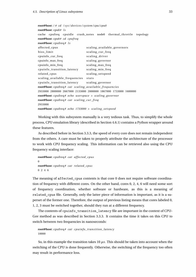
4.5. Description of Linux subsystems 33
root@host : / # cd / s y s / devices / system / cpu / cpu0
root@host : cpu0# l s
cache cpufreq cpuidle crash_notes node0 thermal_thrott le topology
root@host : cpu0# cd cpufreq
root@host : cpufreq# l s
affected_cpus scaling_available_governors
bios_l imit scaling_cur_freq
cpuinfo_cur_freq scal i ng_ dr iv e r
cpuinfo_max_freq scaling_governor
cpuinfo_min_freq scaling_max_freq
cpuinfo_transit ion_latency scaling_min_freq
related_cpus scaling_setspeed
scal ing_avai lable_frequencies s t a t s
cpuinfo_transit ion_latency scaling_governor
root@host : cpufreq# cat scal ing_avai l able_fre que ncies
2933000 2800000 2667000 2133000 2000000 1867000 1733000 1600000
root@host : cpufreq# echo userspace > scaling_governor
root@host : cpufreq# cat scal ing_cur_freq
2933000
root@host : cpufreq# echo 1733000 > scal ing_setspeed
Working with this subsystem manually is a very tedious task. Thus, to simplify the whole
process, CPU emulation library (described in Section 4.6.1) contains a Python wrapper around
these features.
As described before in Section 3.3.3, the speed of every core does not remain independent
from the others. A care must be taken to properly attribute the architecture of the processor
to work with CPU frequency scaling. This information can be retrieved also using the CPU
frequency scaling interface:
root@host : cpufreq# cat affected_cpus
0
root@host : cpufreq# cat related_cpus
0 2 4 6
The meaning of affected_cpus contents is that core 0 does not require software coordina-
tion of frequency with different cores. On the other hand, cores 0, 2, 4, 6 will need some sort
of frequency coordination, whether software or hardware, as this is a meaning of
related_cpus file. Generally, only the latter piece of information is important, as it is a su-
perset of the former one. Therefore, the output of previous listing means that cores labeled 0,
1, 2, 3 must be switched together, should they run at a different frequency.
The contents of cpuinfo_transition_latency file are important in the context of CPU-
Gov method as was described in Section 3.3.3. It contains the time it takes on this CPU to
switch between two frequencies in nanoseconds:
root@host : cpufreq# cat cpuinfo_transit ion_latency
10000
So, in this example the transition takes 10 µs. This should be taken into account when the
switching of the CPU is done frequently. Otherwise, the switching of the frequency too often
may result in performance loss.
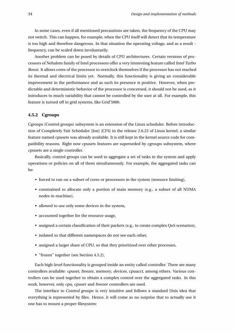
34 Design and implementation of methods
In some cases, even if all mentioned precautions are taken, the frequency of the CPU may
not switch. This can happen, for example, when the CPU itself will detect that its temperature
is too high and therefore dangerous. In that situation the operating voltage, and as a result -
frequency, can be scaled down involuntarily.
Another problem can be posed by details of CPU architectures. Certain versions of pro-
cessors of Nehalem family of Intel processors offer a very interesting feature called Intel Turbo
Boost. It allows cores of the processor to overclock themselves if the processor has not reached
its thermal and electrical limits yet. Normally, this functionality is giving an considerable
improvement in the performance and as such its presence is positive. However, when pre-
dictable and deterministic behavior of the processor is concerned, it should not be used, as it
introduces to much variability that cannot be controlled by the user at all. For example, this
feature is turned off in grid systems, like Grid’5000.
4.5.2 Cgroups
Cgroups (Control groups) subsystem is an extension of the Linux scheduler. Before introduc-
tion of Completely Fair Scheduler [Jon] [CFS] in the release 2.6.23 of Linux kernel, a similar
feature named cpusets was already available. It is still kept in the kernel source code for com-
patibility reasons. Right now cpusets features are superseded by cgroups subsystem, where
cpusets are a single controller.
Basically, control groups can be used to aggregate a set of tasks in the system and apply
operations or policies on all of them simultaneously. For example, the aggregated tasks can
be:
• forced to run on a subset of cores or processors in the system (resource limiting),
• constrained to allocate only a portion of main memory (e.g., a subset of all NUMA
nodes in machine),
• allowed to use only some devices in the system,
• accounted together for the resource usage,
• assigned a certain classification of their packets (e.g., to create complex QoS scenarios),
• isolated so that different namespaces do not see each other,
• assigned a larger share of CPU, so that they prioritized over other processes,
• "frozen" together (see Section 4.5.2),
Each high-level functionality is grouped inside an entity called controller. There are many
controllers available: cpuset, freezer, memory, devices, cpuacct, among others. Various con-
trollers can be used together to obtain a complex control over the aggregated tasks. In this
work, however, only cpu, cpuset and freezer controllers are used.
The interface to Control groups is very intuitive and follows a standard Unix idea that
everything is represented by files. Hence, it will come as no surprise that to actually use it
one has to mount a proper filesystem:
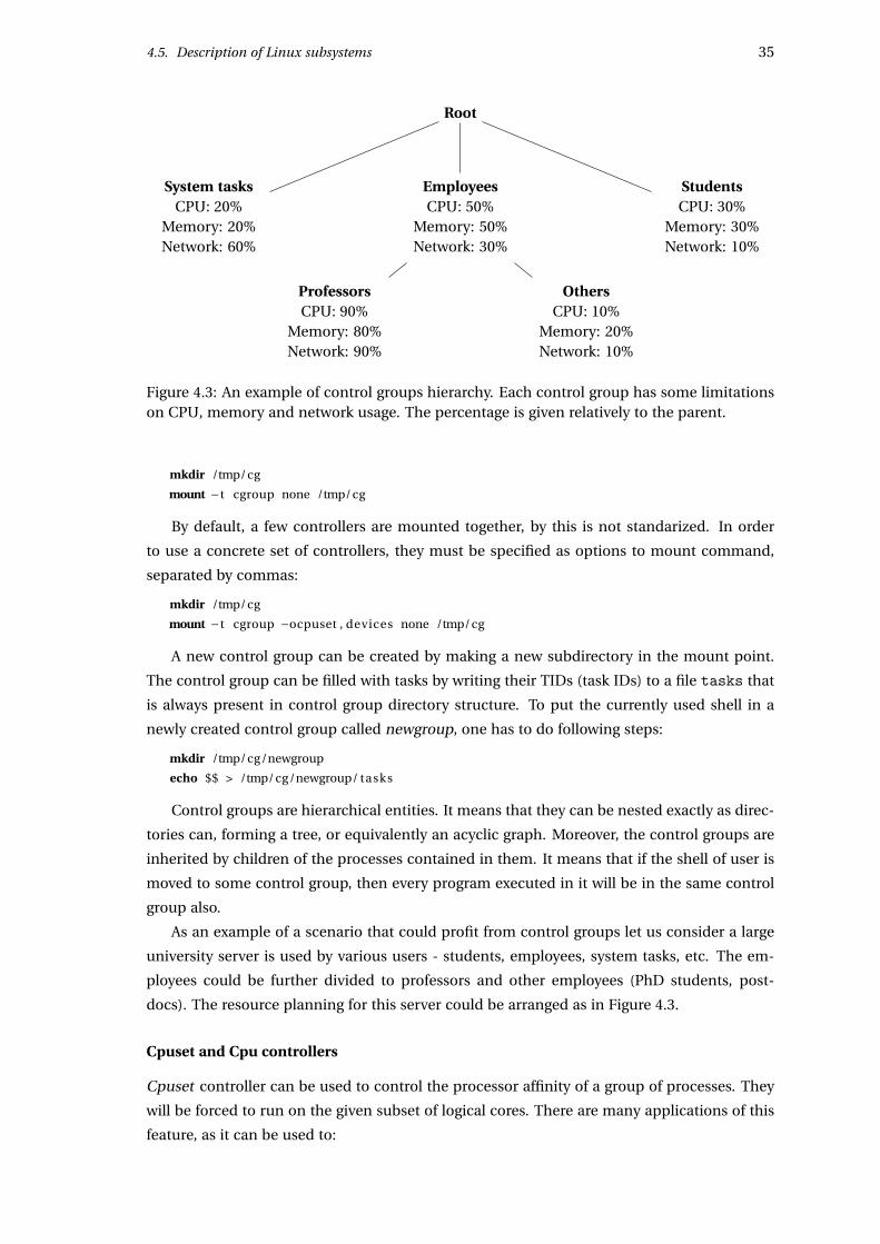
4.5. Description of Linux subsystems 35
Root
System tasksCPU: 20%
Memory: 20%Network: 60%
EmployeesCPU: 50%
Memory: 50%Network: 30%
ProfessorsCPU: 90%
Memory: 80%Network: 90%
OthersCPU: 10%
Memory: 20%Network: 10%
StudentsCPU: 30%
Memory: 30%Network: 10%
Figure 4.3: An example of control groups hierarchy. Each control group has some limitationson CPU, memory and network usage. The percentage is given relatively to the parent.
mkdir /tmp/cg
mount −t cgroup none /tmp/cg
By default, a few controllers are mounted together, by this is not standarized. In order
to use a concrete set of controllers, they must be specified as options to mount command,
separated by commas:
mkdir /tmp/cg
mount −t cgroup −ocpuset , devices none /tmp/cg
A new control group can be created by making a new subdirectory in the mount point.
The control group can be filled with tasks by writing their TIDs (task IDs) to a file tasks that
is always present in control group directory structure. To put the currently used shell in a
newly created control group called newgroup, one has to do following steps:
mkdir /tmp/cg/newgroup
echo $$ > /tmp/cg/newgroup/ tasks
Control groups are hierarchical entities. It means that they can be nested exactly as direc-
tories can, forming a tree, or equivalently an acyclic graph. Moreover, the control groups are
inherited by children of the processes contained in them. It means that if the shell of user is
moved to some control group, then every program executed in it will be in the same control
group also.
As an example of a scenario that could profit from control groups let us consider a large
university server is used by various users - students, employees, system tasks, etc. The em-
ployees could be further divided to professors and other employees (PhD students, post-
docs). The resource planning for this server could be arranged as in Figure 4.3.
Cpuset and Cpu controllers
Cpuset controller can be used to control the processor affinity of a group of processes. They
will be forced to run on the given subset of logical cores. There are many applications of this
feature, as it can be used to:
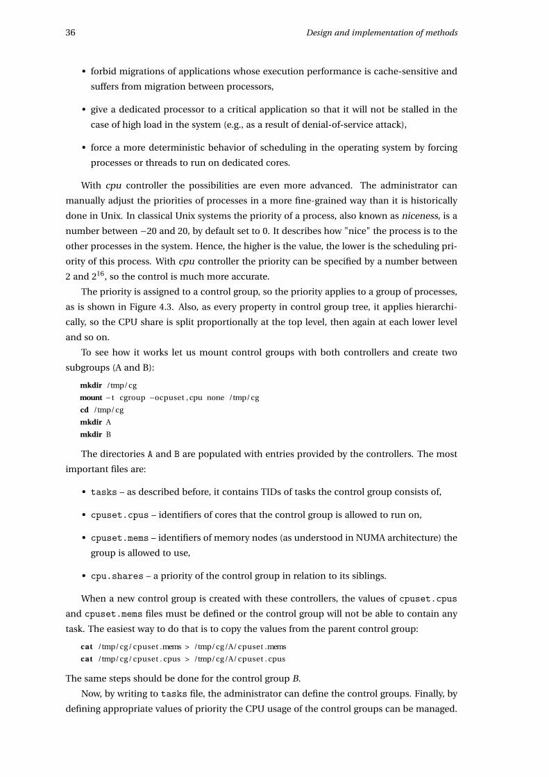
36 Design and implementation of methods
• forbid migrations of applications whose execution performance is cache-sensitive and
suffers from migration between processors,
• give a dedicated processor to a critical application so that it will not be stalled in the
case of high load in the system (e.g., as a result of denial-of-service attack),
• force a more deterministic behavior of scheduling in the operating system by forcing
processes or threads to run on dedicated cores.
With cpu controller the possibilities are even more advanced. The administrator can
manually adjust the priorities of processes in a more fine-grained way than it is historically
done in Unix. In classical Unix systems the priority of a process, also known as niceness, is a
number between −20 and 20, by default set to 0. It describes how "nice" the process is to the
other processes in the system. Hence, the higher is the value, the lower is the scheduling pri-
ority of this process. With cpu controller the priority can be specified by a number between
2 and 216, so the control is much more accurate.
The priority is assigned to a control group, so the priority applies to a group of processes,
as is shown in Figure 4.3. Also, as every property in control group tree, it applies hierarchi-
cally, so the CPU share is split proportionally at the top level, then again at each lower level
and so on.
To see how it works let us mount control groups with both controllers and create two
subgroups (A and B):
mkdir /tmp/cg
mount −t cgroup −ocpuset , cpu none /tmp/cg
cd /tmp/cg
mkdir A
mkdir B
The directories A and B are populated with entries provided by the controllers. The most
important files are:
• tasks – as described before, it contains TIDs of tasks the control group consists of,
• cpuset.cpus – identifiers of cores that the control group is allowed to run on,
• cpuset.mems – identifiers of memory nodes (as understood in NUMA architecture) the
group is allowed to use,
• cpu.shares – a priority of the control group in relation to its siblings.
When a new control group is created with these controllers, the values of cpuset.cpus
and cpuset.mems files must be defined or the control group will not be able to contain any
task. The easiest way to do that is to copy the values from the parent control group:
cat /tmp/cg/ cpuset .mems > /tmp/cg/A/ cpuset .mems
cat /tmp/cg/ cpuset . cpus > /tmp/cg/A/ cpuset . cpus
The same steps should be done for the control group B.
Now, by writing to tasks file, the administrator can define the control groups. Finally, by
defining appropriate values of priority the CPU usage of the control groups can be managed.
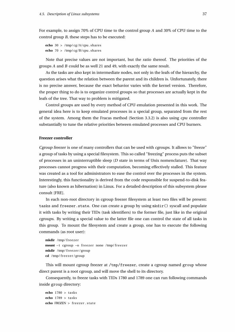
4.5. Description of Linux subsystems 37
For example, to assign 70% of CPU time to the control group A and 30% of CPU time to the
control group B, these steps has to be executed:
echo 30 > /tmp/cg/A/cpu . shares
echo 70 > /tmp/cg/B/cpu . shares
Note that precise values are not important, but the ratio thereof. The priorities of the
groups A and B could be as well 21 and 49, with exactly the same result.
As the tasks are also kept in intermediate nodes, not only in the leafs of the hierarchy, the
question arises what the relation between the parent and its children is. Unfortunately, there
is no precise answer, because the exact behavior varies with the kernel version. Therefore,
the proper thing to do is to organize control groups so that processes are actually kept in the
leafs of the tree. That way to problem is mitigated.
Control groups are used by every method of CPU emulation presented in this work. The
general idea here is to keep emulated processes in a special group, separated from the rest
of the system. Among them the Fracas method (Section 3.3.2) is also using cpu controller
substantially to tune the relative priorities between emulated processes and CPU burners.
Freezer controller
Cgroup freezer is one of many controllers that can be used with cgroups. It allows to "freeze"
a group of tasks by using a special filesystem. This so called "freezing" process puts the subset
of processes in an uninterruptible sleep (D state in terms of Unix nomenclature). That way
processes cannot progress with their computation, becoming effectively stalled. This feature
was created as a tool for administrators to ease the control over the processes in the system.
Interestingly, this functionality is derived from the code responsible for suspend-to-disk fea-
ture (also known as hibernation) in Linux. For a detailed description of this subsystem please
consult [FRE].
In each non-root directory in cgroup freezer filesystem at least two files will be present:
tasks and freezer.state. One can create a group by using mkdir() syscall and populate
it with tasks by writing their TIDs (task identifiers) to the former file, just like in the original
cgroups. By writing a special value to the latter file one can control the state of all tasks in
this group. To mount the filesystem and create a group, one has to execute the following
commands (as root user):
mkdir /tmp/ free ze r
mount −t cgroup −o fr ee ze r none /tmp/ fre ez er
mkdir /tmp/ free ze r /group
cd /tmp/ free ze r /group
This will mount cgroup freezer at /tmp/freezer, create a cgroup named group whose
direct parent is a root cgroup, and will move the shell to its directory.
Consequently, to freeze tasks with TIDs 1780 and 1789 one can run following commands
inside group directory:
echo 1780 > tasks
echo 1789 > tasks
echo FROZEN > fr eez er . s t a t e
38 Design and implementation of methods
After these commands the tasks will remain in uninterruptible state until the administra-
tor will "thaw" them:
echo THAWED > fre ez er . s t a t e
The status of a cgroup can be checked at any time by reading a file freezer.state.
When the task is in the uninterruptible state it is not considered by the system scheduler.
Normally, this state of a task is temporary, experienced during a sensitive operation which
cannot be interrupted for some technical reason, sometimes related to the hardware. As a
result the task cannot be killed by SIGKILL signal, even by the administrator. The task will
hold its acquired resources until it is finally unblocked. Cgroup freezer gives an ability to put
any task in that state for a desired period of time.
During this work, bugs with this part of the Linux kernel were found. They are described
in Section 4.7.2.
The control groups freezer is used extensively by CPU-Gov method. Normally, when the
emulated frequency can be emulated by means of frequency level exposed by the hardware,
it is not needed. If, on the other hand, the emulated frequency is lower than the lowest hard-
ware frequency level, then freezing is used to simulate zero frequency level.
4.6 Description of the implementation
In this section, the important details of the implementation are discussed.
4.6.1 CPU emulation library
At the beginning all methods of CPU emulation were separately written and maintained. As a
result a lot of the code was redundant and a lot of functionality duplicated in different places.
As a result, the code base was becoming unmaintainable.
Thus, at some point a decision was made to extract all common functionality needed by
the methods. This includes:
• managing the frequency of cores in the system,
• allocating CPU cores with and without considering their architectural relations,
• managing the control groups, their priorities and tasks,
• setting real-time priorities of the processes,
• managing execution of CPU emulation methods,
• keeping the user interface consistent.
The result of this refactoring is a Python library called cpuemu. All methods, or at least
their frontends, use this library to keep the implementation details of all methods consistent
with each other as much as possible. As a side affect, the previous implementation of the
methods became much shorter, in most cases not exceeding two pages of Python code.
The cpuemu library provides also three different core allocation strategies for virtual nodes:
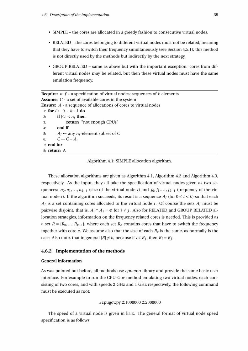
4.6. Description of the implementation 39
• SIMPLE – the cores are allocated in a greedy fashion to consecutive virtual nodes,
• RELATED – the cores belonging to different virtual nodes must not be related, meaning
that they have to switch their frequency simultaneously (see Section 4.5.1); this method
is not directly used by the methods but indirectly by the next strategy,
• GROUP RELATED – same as above but with the important exception: cores from dif-
ferent virtual nodes may be related, but then these virtual nodes must have the same
emulation frequency.
Require: n, f - a specification of virtual nodes; sequences of k elementsAssume: C - a set of available cores in the systemEnsure: A - a sequence of allocations of cores to virtual nodes
1: for i ← 0. . .k −1 do2: if |C | < ni then3: return "not enough CPUs"4: end if5: Ai ← any ni -element subset of C6: C ←C − Ai
7: end for8: return A
Algorithm 4.1: SIMPLE allocation algorithm.
These allocation algorithms are given as Algorithm 4.1, Algorithm 4.2 and Algorithm 4.3,
respectively. As the input, they all take the specification of virtual nodes given as two se-
quences: n0,n1, . . . ,nk−1 (size of the virtual node i ) and f0, f1, . . . , fk−1 (frequency of the vir-
tual node i ). If the algorithm succeeds, its result is a sequence Ai (for 0 ≤ i < k) so that each
Ai is a set containing cores allocated to the virtual node i . Of course the sets Ai must be
pairwise disjoint, that is, Ai ∩ A j = ; for i 6= j . Also for RELATED and GROUP RELATED al-
location strategies, information on the frequency related cores is needed. This is provided as
a set R = {R0, . . . ,Rk−1}, where each set Rc contains cores that have to switch the frequency
together with core c. We assume also that the size of each Rc is the same, as normally is the
case. Also note, that in general |R| 6= k, because if i ∈ R j , then Ri = R j .
4.6.2 Implementation of the methods
General information
As was pointed out before, all methods use cpuemu library and provide the same basic user
interface. For example to run the CPU-Gov method emulating two virtual nodes, each con-
sisting of two cores, and with speeds 2 GHz and 1 GHz respectively, the following command
must be executed as root:
./cpugov.py 2:1000000 2:2000000
The speed of a virtual node is given in kHz. The general format of virtual node speed
specification is as follows:
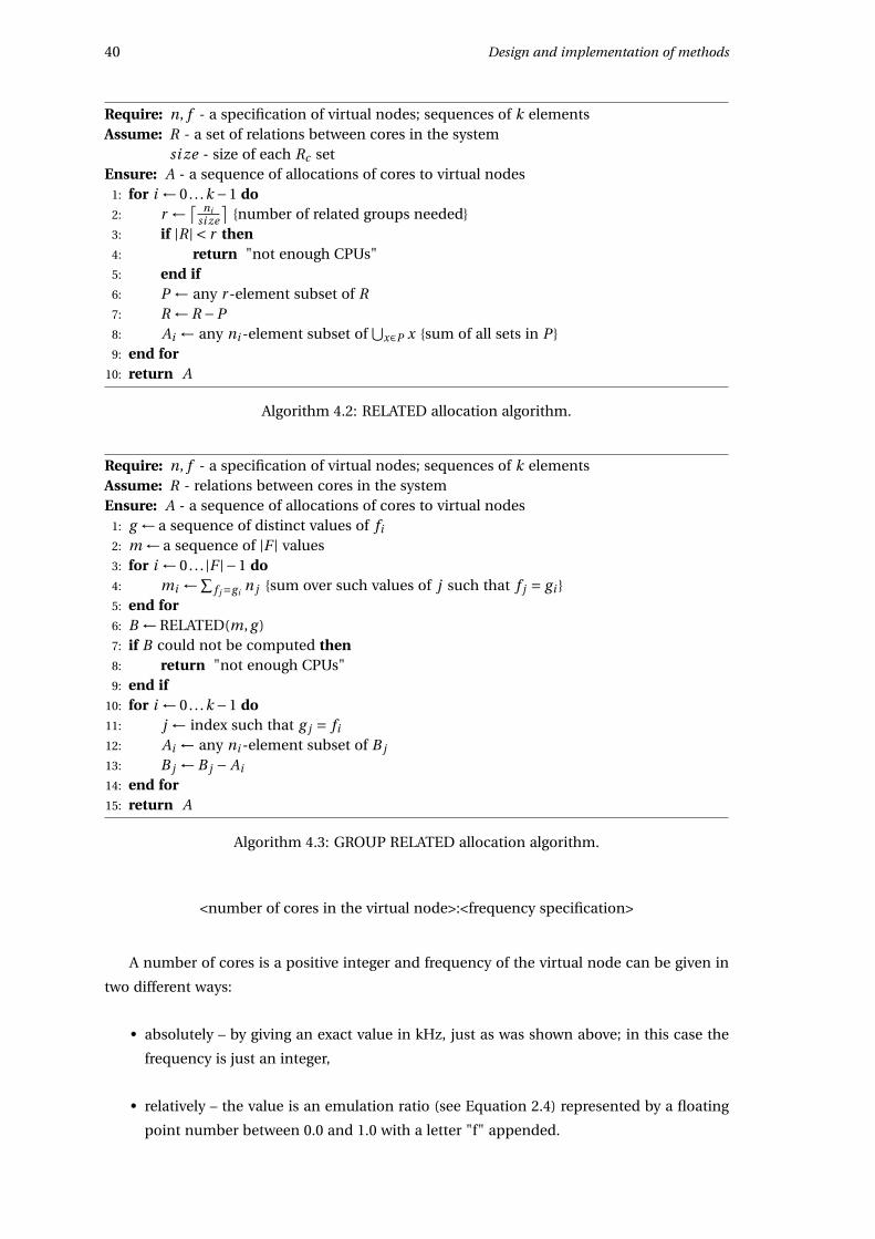
40 Design and implementation of methods
Require: n, f - a specification of virtual nodes; sequences of k elementsAssume: R - a set of relations between cores in the systemAssume: si ze - size of each Rc setEnsure: A - a sequence of allocations of cores to virtual nodes
1: for i ← 0. . .k −1 do2: r ← ⌈ ni
si ze
⌉{number of related groups needed}
3: if |R| < r then4: return "not enough CPUs"5: end if6: P ← any r -element subset of R7: R ← R −P8: Ai ← any ni -element subset of
⋃x∈P x {sum of all sets in P }
9: end for10: return A
Algorithm 4.2: RELATED allocation algorithm.
Require: n, f - a specification of virtual nodes; sequences of k elementsAssume: R - relations between cores in the systemEnsure: A - a sequence of allocations of cores to virtual nodes
1: g ← a sequence of distinct values of fi
2: m ← a sequence of |F | values3: for i ← 0. . . |F |−1 do4: mi ←∑
f j=gin j {sum over such values of j such that f j = gi }
5: end for6: B ← RELATED(m, g )7: if B could not be computed then8: return "not enough CPUs"9: end if
10: for i ← 0. . .k −1 do11: j ← index such that g j = fi
12: Ai ← any ni -element subset of B j
13: B j ← B j − Ai
14: end for15: return A
Algorithm 4.3: GROUP RELATED allocation algorithm.
<number of cores in the virtual node>:<frequency specification>
A number of cores is a positive integer and frequency of the virtual node can be given in
two different ways:
• absolutely – by giving an exact value in kHz, just as was shown above; in this case the
frequency is just an integer,
• relatively – the value is an emulation ratio (see Equation 2.4) represented by a floating
point number between 0.0 and 1.0 with a letter "f" appended.
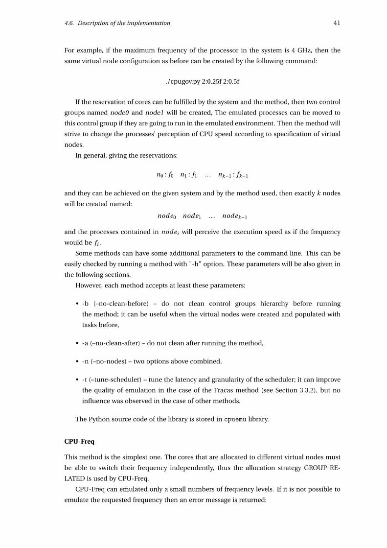
4.6. Description of the implementation 41
For example, if the maximum frequency of the processor in the system is 4 GHz, then the
same virtual node configuration as before can be created by the following command:
./cpugov.py 2:0.25f 2:0.5f
If the reservation of cores can be fulfilled by the system and the method, then two control
groups named node0 and node1 will be created, The emulated processes can be moved to
this control group if they are going to run in the emulated environment. Then the method will
strive to change the processes’ perception of CPU speed according to specification of virtual
nodes.
In general, giving the reservations:
n0 : f0 n1 : f1 . . . nk−1 : fk−1
and they can be achieved on the given system and by the method used, then exactly k nodes
will be created named:
node0 node1 . . . nodek−1
and the processes contained in nodei will perceive the execution speed as if the frequency
would be fi .
Some methods can have some additional parameters to the command line. This can be
easily checked by running a method with "-h" option. These parameters will be also given in
the following sections.
However, each method accepts at least these parameters:
• -b (–no-clean-before) – do not clean control groups hierarchy before running
the method; it can be useful when the virtual nodes were created and populated with
tasks before,
• -a (–no-clean-after) – do not clean after running the method,
• -n (–no-nodes) – two options above combined,
• -t (–tune-scheduler) – tune the latency and granularity of the scheduler; it can improve
the quality of emulation in the case of the Fracas method (see Section 3.3.2), but no
influence was observed in the case of other methods.
The Python source code of the library is stored in cpuemu library.
CPU-Freq
This method is the simplest one. The cores that are allocated to different virtual nodes must
be able to switch their frequency independently, thus the allocation strategy GROUP RE-
LATED is used by CPU-Freq.
CPU-Freq can emulated only a small numbers of frequency levels. If it is not possible to
emulate the requested frequency then an error message is returned:
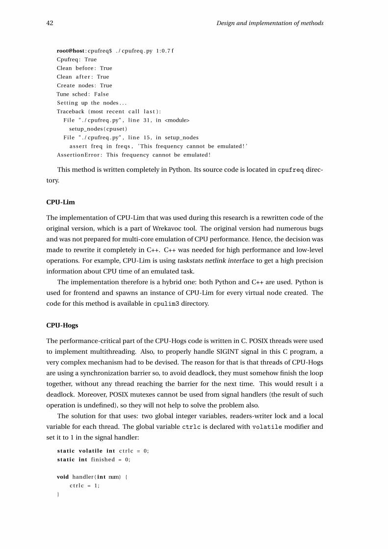
42 Design and implementation of methods
root@host : cpufreq$ . / cpufreq . py 1 : 0 . 7 f
Cpufreq : True
Clean before : True
Clean a f t e r : True
Create nodes : True
Tune sched : False
Sett ing up the nodes . . .
Traceback ( most recent c a l l l a s t ) :
F i l e " . / cpufreq . py" , l i n e 31 , in <module>
setup_nodes ( cpuset )
F i l e " . / cpufreq . py" , l i n e 15 , in setup_nodes
a s s e r t freq in freqs , ’ This frequency cannot be emulated ! ’
AssertionError : This frequency cannot be emulated !
This method is written completely in Python. Its source code is located in cpufreq direc-
tory.
CPU-Lim
The implementation of CPU-Lim that was used during this research is a rewritten code of the
original version, which is a part of Wrekavoc tool. The original version had numerous bugs
and was not prepared for multi-core emulation of CPU performance. Hence, the decision was
made to rewrite it completely in C++. C++ was needed for high performance and low-level
operations. For example, CPU-Lim is using taskstats netlink interface to get a high precision
information about CPU time of an emulated task.
The implementation therefore is a hybrid one: both Python and C++ are used. Python is
used for frontend and spawns an instance of CPU-Lim for every virtual node created. The
code for this method is available in cpulim3 directory.
CPU-Hogs
The performance-critical part of the CPU-Hogs code is written in C. POSIX threads were used
to implement multithreading. Also, to properly handle SIGINT signal in this C program, a
very complex mechanism had to be devised. The reason for that is that threads of CPU-Hogs
are using a synchronization barrier so, to avoid deadlock, they must somehow finish the loop
together, without any thread reaching the barrier for the next time. This would result i a
deadlock. Moreover, POSIX mutexes cannot be used from signal handlers (the result of such
operation is undefined), so they will not help to solve the problem also.
The solution for that uses: two global integer variables, readers-writer lock and a local
variable for each thread. The global variable ctrlc is declared with volatile modifier and
set it to 1 in the signal handler:
s t a t i c v o l a t i l e int c t r l c = 0 ;
s t a t i c int f inished = 0 ;
void handler ( int num) {
c t r l c = 1 ;
}
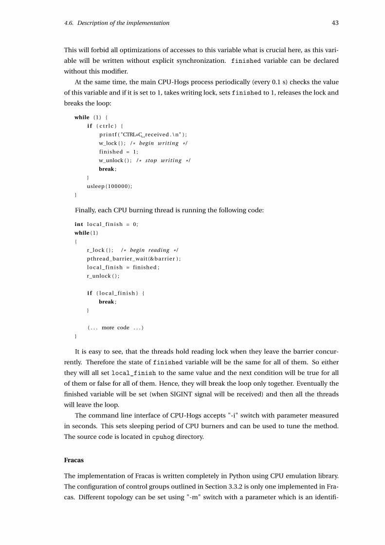
4.6. Description of the implementation 43
This will forbid all optimizations of accesses to this variable what is crucial here, as this vari-
able will be written without explicit synchronization. finished variable can be declared
without this modifier.
At the same time, the main CPU-Hogs process periodically (every 0.1 s) checks the value
of this variable and if it is set to 1, takes writing lock, sets finished to 1, releases the lock and
breaks the loop:
while ( 1 ) {
i f ( c t r l c ) {
p r i n t f ( "CTRL+C received . \ n" ) ;
w_lock ( ) ; / * begin writing * /
f inished = 1 ;
w_unlock ( ) ; / * stop writing * /
break ;
}
usleep (100000);
}
Finally, each CPU burning thread is running the following code:
int l o c a l _ f i n i s h = 0 ;
while ( 1 )
{
r_lock ( ) ; / * begin reading * /
pthread_barrier_wait (& b a r r i e r ) ;
l o c a l _ f i n i s h = finished ;
r_unlock ( ) ;
i f ( l o c a l _ f i n i s h ) {
break ;
}
( . . . more code . . . )
}
It is easy to see, that the threads hold reading lock when they leave the barrier concur-
rently. Therefore the state of finished variable will be the same for all of them. So either
they will all set local_finish to the same value and the next condition will be true for all
of them or false for all of them. Hence, they will break the loop only together. Eventually the
finished variable will be set (when SIGINT signal will be received) and then all the threads
will leave the loop.
The command line interface of CPU-Hogs accepts "-i" switch with parameter measured
in seconds. This sets sleeping period of CPU burners and can be used to tune the method.
The source code is located in cpuhog directory.
Fracas
The implementation of Fracas is written completely in Python using CPU emulation library.
The configuration of control groups outlined in Section 3.3.2 is only one implemented in Fra-
cas. Different topology can be set using "-m" switch with a parameter which is an identifi-
44 Design and implementation of methods
cation number of a topology of control groups. In some cases they may give better results.
There as much as 8 different topologies implemented.
The source code of Fracas is in fracas directory.
CPU-Gov
CPU-Gov is completely written in Python. The future actions, i.e., changes to the frequency of
CPUs are stored on a priority queue implemented as a heap. The elements are conceptually
of the form (t ,c, f ) where:
• t - the time in the future when this event will happen,
• c - a set of cores whose frequency will change,
• f - the frequency to set when the event happens.
CPU-Gov periodically sleeps till the time the next event in the queue should be executed.
Then the event is taken from the queue the frequency of cores is adjusted properly. Finally,
the event is updated with new values of t and f and returned to the priority queue.
It is a very clean algorithm with few advantages:
• the main process runs only when needed, minimizing the load it generates,
• the drift of clock does not influence the computation,
• them method scales very well with the number of virtual nodes, as the heap operations
have complexity of O(log n).
A solution for "zero frequency" problem described in Section 4.6.2, resonating with cgroup
design is provided by Cgroup freezer. This subsystem was already described in Section 4.5.2.
Unfortunately, some problems were encountered as described in Section 4.7.2.
Similarly to the CPU-Hogs method, this method can also be adjusted with "-i" switch
which controls the length of a switching period.
The source code of this method is in cpugov directory.
4.6.3 Distributed testing framework
Distest is a framework used extensively to evaluate the methods presented in this paper. It
is possible to run many tests concurrently on the cluster, improving the speed of evaluation
by one order of magnitude. Also the reproducibility of the results is assured, since the exper-
iment is described inside a single file.
Distest consists of:
• a server – it holds the description of the whole experiment, distributes the jobs to clients,
manages (stores) the results and does a final processing of them,
• a client – a single node in the cluster that connects to the server, executes an instance
of experiment task, and returns the result.
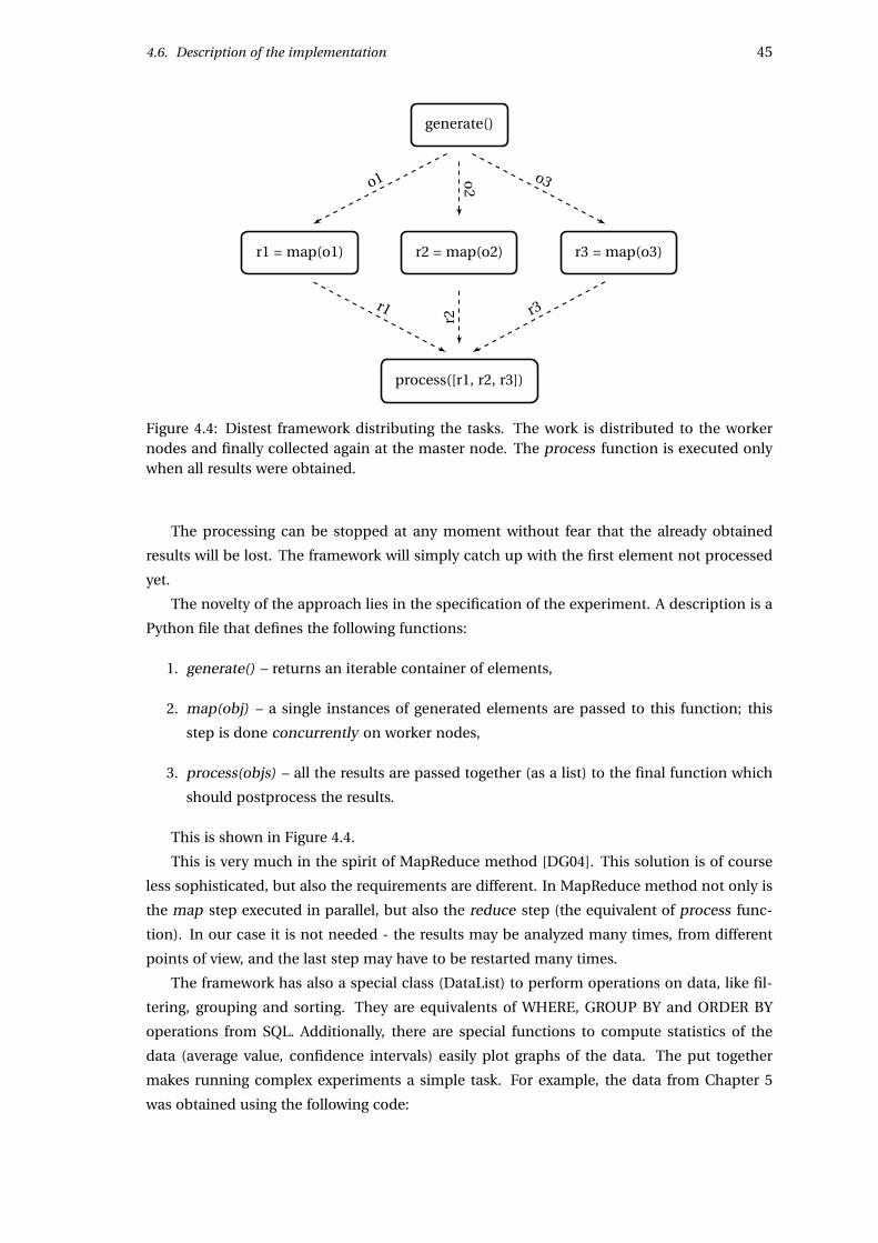
4.6. Description of the implementation 45
generate()
r2 = map(o2)r1 = map(o1) r3 = map(o3)
process([r1, r2, r3])
o1 o2
o3
r1
r2 r3
Figure 4.4: Distest framework distributing the tasks. The work is distributed to the workernodes and finally collected again at the master node. The process function is executed onlywhen all results were obtained.
The processing can be stopped at any moment without fear that the already obtained
results will be lost. The framework will simply catch up with the first element not processed
yet.
The novelty of the approach lies in the specification of the experiment. A description is a
Python file that defines the following functions:
1. generate() – returns an iterable container of elements,
2. map(obj) – a single instances of generated elements are passed to this function; this
step is done concurrently on worker nodes,
3. process(objs) – all the results are passed together (as a list) to the final function which
should postprocess the results.
This is shown in Figure 4.4.
This is very much in the spirit of MapReduce method [DG04]. This solution is of course
less sophisticated, but also the requirements are different. In MapReduce method not only is
the map step executed in parallel, but also the reduce step (the equivalent of process func-
tion). In our case it is not needed - the results may be analyzed many times, from different
points of view, and the last step may have to be restarted many times.
The framework has also a special class (DataList) to perform operations on data, like fil-
tering, grouping and sorting. They are equivalents of WHERE, GROUP BY and ORDER BY
operations from SQL. Additionally, there are special functions to compute statistics of the
data (average value, confidence intervals) easily plot graphs of the data. The put together
makes running complex experiments a simple task. For example, the data from Chapter 5
was obtained using the following code:
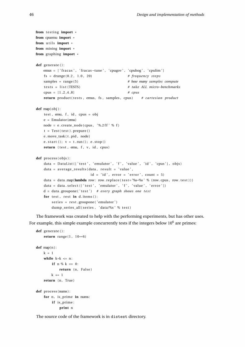
46 Design and implementation of methods
from t e s t i n g import *from cpuemu import *from u t i l s import *from mining import *from graphing import *
def generate ( ) :
emus = [ ’ fracas ’ , ’ fracas−tune ’ , ’ cpugov ’ , ’cpuhog ’ , ’ cpulim ’ ]
f s = drange ( 0 . 2 , 1 . 0 , 20) # frequency s t e p s
samples = range ( 5 ) # how many samples compute
t e s t s = l i s t (TESTS) # take ALL micro−benchmarks
cpus = [ 1 , 2 , 4 , 8 ] # cpus
return product ( t e s t s , emus, fs , samples , cpus ) # cartesian product
def map( obj ) :
test , emu, f , id , cpus = obj
e = Emulator (emu)
node = e . create_node ( cpus , ’ %.2 f f ’ % f )
t = Test ( t e s t ) . prepare ( )
e . move_task ( t . pid , node)
e . s t a r t ( ) ; v = t . run ( ) ; e . stop ( )
return ( test , emu, f , v , id , cpus )
def process ( objs ) :
data = DataList ( [ ’ t e s t ’ , ’ emulator ’ , ’ f ’ , ’ value ’ , ’ id ’ , ’ cpus ’ ] , objs )
data = average_results ( data , r e s u l t = ’ value ’ ,
id = ’ id ’ , error = ’ error ’ , count = 5)
data = data .map( lambda row : row . replace ( t e s t = ’%s−%s ’ % (row . cpus , row . t e s t ) ) )
data = data . s e l e c t ( [ ’ t e s t ’ , ’ emulator ’ , ’ f ’ , ’ value ’ , ’ error ’ ] )
d = data . groupone ( ’ t e s t ’ ) # every graph shows one t e s t
for test , r e s t in d . items ( ) :
s e r i e s = r e s t . groupone ( ’ emulator ’ )
dump_series_all ( ser ies , ’ data/%s ’ % t e s t )
The framework was created to help with the performing experiments, but has other uses.
For example, this simple example concurrently tests if the integers below 106 are primes:
def generate ( ) :
return range ( 1 , 10**6)
def map(n ) :
k = 1
while k*k <= n :
i f n % k == 0 :
return (n , False )
k += 1
return (n , True )
def process (nums ) :
for n , is_prime in nums:
i f is_prime :
print n
The source code of the framework is in distest directory.
4.7. Problems encountered 47
4.7 Problems encountered
4.7.1 Problems with Grid’5000
The majority of experiments concerned in this thesis was carried out on the Grid’5000 testbed
[G5K]. This is going to be described in much more details in the Section 5.3, but was also a
source of some problems. More concretely, 4 major problems were observed:
• SSH keys management and connection tunnelling,
• connectivity problems from outside of the workplace,
• synchronization of data between the sites,
• issues with NFS servers.
They will be described in that order.
The workflow with Grid’5000 usually consists of the following steps (see solid arrows in
Figure 4.5):
1. Connect to any site via its frontend.
2. Optionally connect to a different site from the current site.
3. Make reservations and wait until they are fulfilled.
4. Connect to the reserved nodes and run the experiment or computation.
The steps 1, 2 and 4 require making SSH connections to various hosts spread throughout
the Grid’5000 network. If the user account is not properly configured this will actually be
required to type the password manually 3 times every possible reservation. This would be to
time consuming and would forbid automated experiments or synchronization of files without
a password.
The generally known solution to the problem is the use of password-less logins. The user
creates a pair of cryptographic public and private keys (either RSA or DSA) locally and then
configures its account on the server side to allow authentication by means of public key cryp-
tography. The following listing presents how this can be achieved:
user@client :~ $ ssh−keygen
Generating public / private rsa key pair .
Enter f i l e in which to save the key ( /home/ user / . ssh / id_rsa ) :
Created directory ’/home/ user / . ssh ’ .
Enter passphrase (empty for no passphrase ) : <no passphrase >
Enter same passphrase again : <no passphrase>
Your i d e n t i f i c a t i o n has been saved in /home/ user / . ssh / id_rsa .
Your public key has been saved in /home/ user / . ssh / id_rsa . pub .
<additional information >
user@client :~ $ ssh−copy−id host
Password : <password>
Now t r y logging into the machine , with " ssh ’ host ’ " , and check in :
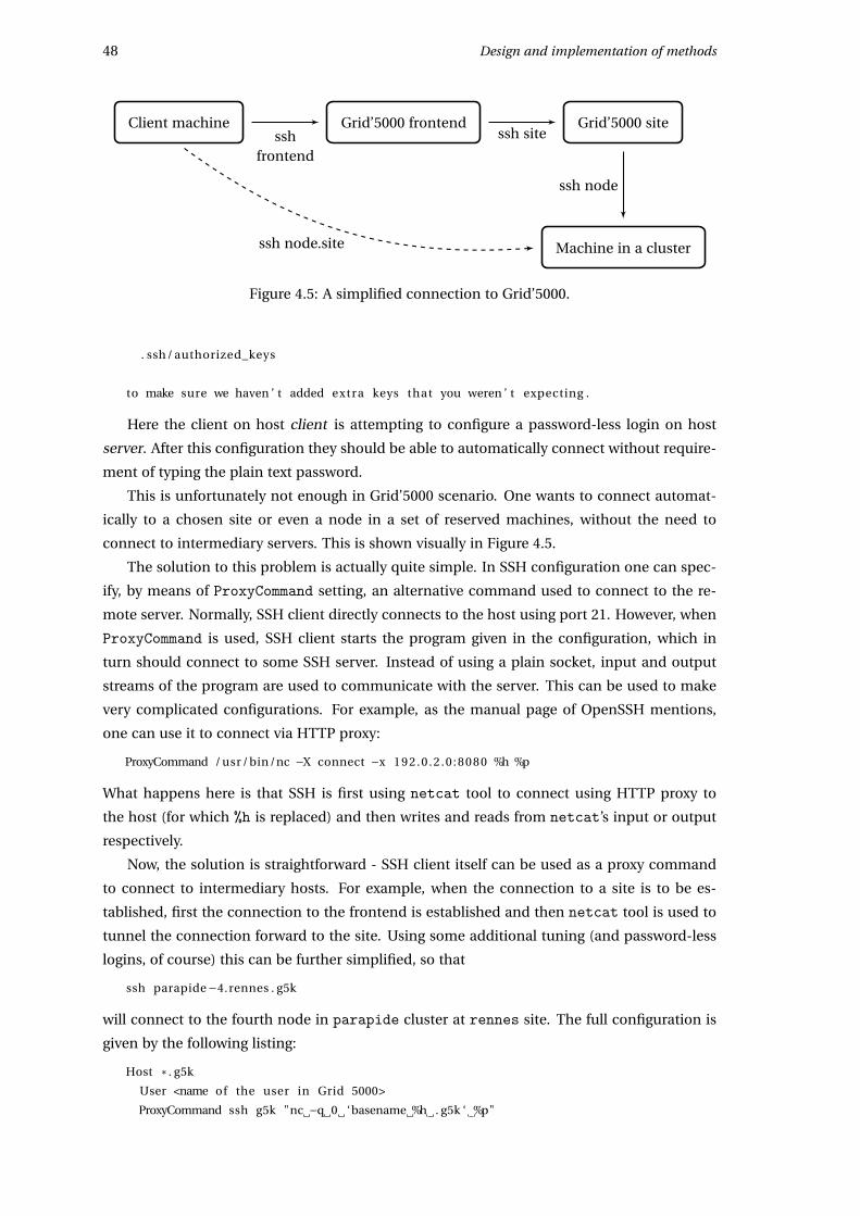
48 Design and implementation of methods
Client machine Grid’5000 frontend Grid’5000 site
Machine in a cluster
sshfrontend
ssh site
ssh node
ssh node.site
Figure 4.5: A simplified connection to Grid’5000.
. ssh / authorized_keys
to make sure we haven ’ t added extra keys that you weren ’ t expecting .
Here the client on host client is attempting to configure a password-less login on host
server. After this configuration they should be able to automatically connect without require-
ment of typing the plain text password.
This is unfortunately not enough in Grid’5000 scenario. One wants to connect automat-
ically to a chosen site or even a node in a set of reserved machines, without the need to
connect to intermediary servers. This is shown visually in Figure 4.5.
The solution to this problem is actually quite simple. In SSH configuration one can spec-
ify, by means of ProxyCommand setting, an alternative command used to connect to the re-
mote server. Normally, SSH client directly connects to the host using port 21. However, when
ProxyCommand is used, SSH client starts the program given in the configuration, which in
turn should connect to some SSH server. Instead of using a plain socket, input and output
streams of the program are used to communicate with the server. This can be used to make
very complicated configurations. For example, as the manual page of OpenSSH mentions,
one can use it to connect via HTTP proxy:
ProxyCommand / usr /bin/nc −X connect −x 192.0 .2 .0 :8080 %h %p
What happens here is that SSH is first using netcat tool to connect using HTTP proxy to
the host (for which %h is replaced) and then writes and reads from netcat’s input or output
respectively.
Now, the solution is straightforward - SSH client itself can be used as a proxy command
to connect to intermediary hosts. For example, when the connection to a site is to be es-
tablished, first the connection to the frontend is established and then netcat tool is used to
tunnel the connection forward to the site. Using some additional tuning (and password-less
logins, of course) this can be further simplified, so that
ssh parapide−4.rennes . g5k
will connect to the fourth node in parapide cluster at rennes site. The full configuration is
given by the following listing:
Host * . g5k
User <name of the user in Grid 5000>
ProxyCommand ssh g5k "nc −q 0 ‘basename %h . g5k ‘ %p"
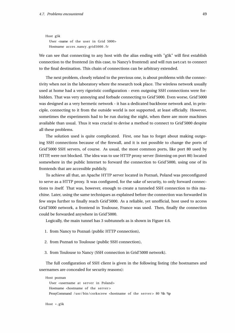
4.7. Problems encountered 49
Host g5k
User <name of the user in Grid 5000>
Hostname acces . nancy . grid5000 . f r
We can see that connecting to any host with the alias ending with "g5k" will first establish
connection to the frontend (in this case, to Nancy’s frontend) and will run netcat to connect
to the final destination. This chain of connections can be arbitrary extended.
The next problem, closely related to the previous one, is about problems with the connec-
tivity when not in the laboratory where the research took place. The wireless network usually
used at home had a very rigoristic configuration - even outgoing SSH connections were for-
bidden. That was very annoying and forbade connecting to Grid’5000. Even worse, Grid’5000
was designed as a very hermetic network - it has a dedicated backbone network and, in prin-
ciple, connecting to it from the outside world is not supported, at least officially. However,
sometimes the experiments had to be run during the night, when there are more machines
available than usual. Thus it was crucial to devise a method to connect to Grid’5000 despite
all these problems.
The solution used is quite complicated. First, one has to forget about making outgo-
ing SSH connections because of the firewall, and it is not possible to change the ports of
Grid’5000 SSH servers, of course. As usual, the most common ports, like port 80 used by
HTTP, were not blocked. The idea was to use HTTP proxy server (listening on port 80) located
somewhere in the public Internet to forward the connection to Grid’5000, using one of its
frontends that are accessible publicly.
To achieve all that, an Apache HTTP server located in Poznan, Poland was preconfigured
to serve as a HTTP proxy. It was configured, for the sake of security, to only forward connec-
tions to itself. That was, however, enough to create a tunneled SSH connection to this ma-
chine. Later, using the same techniques as explained before the connection was forwarded in
few steps further to finally reach Grid’5000. As a reliable, yet unofficial, host used to access
Grid’5000 network, a frontend in Toulouse, France was used. Then, finally the connection
could be forwarded anywhere in Grid’5000.
Logically, the main tunnel has 3 subtunnels as is shown in Figure 4.6.
1. from Nancy to Poznan (public HTTP connection),
2. from Poznan to Toulouse (public SSH connection),
3. from Toulouse to Nancy (SSH connection in Grid’5000 network).
The full configuration of SSH client is given in the following listing (the hostnames and
usernames are concealed for security reasons):
Host poznan
User <username at server in Poland>
Hostname <hostname of the server >
ProxyCommand / usr /bin/ corkscrew <hostname of the server > 80 %h %p
Host * . g5k
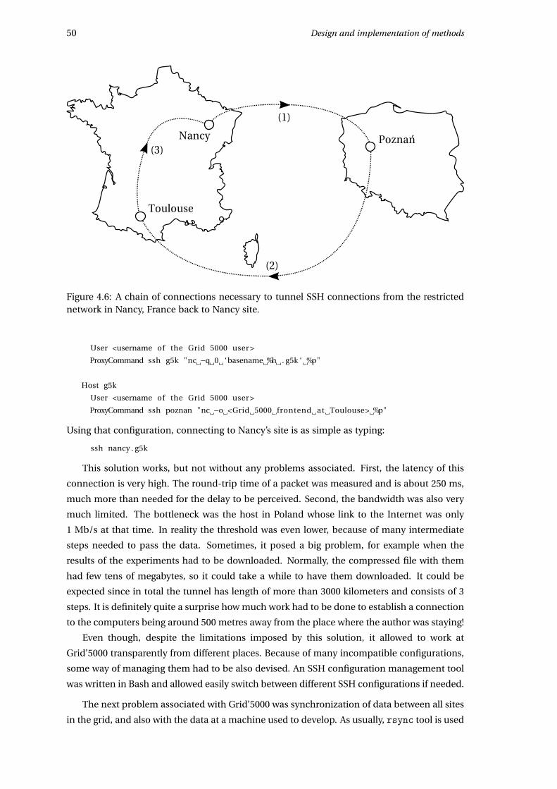
50 Design and implementation of methods
(1)
(2)
(3)
Toulouse
PoznanNancy
Figure 4.6: A chain of connections necessary to tunnel SSH connections from the restrictednetwork in Nancy, France back to Nancy site.
User <username of the Grid 5000 user >
ProxyCommand ssh g5k "nc −q 0 ‘basename %h . g5k ‘ %p"
Host g5k
User <username of the Grid 5000 user >
ProxyCommand ssh poznan "nc −o <Grid 5000 frontend at Toulouse> %p"
Using that configuration, connecting to Nancy’s site is as simple as typing:
ssh nancy . g5k
This solution works, but not without any problems associated. First, the latency of this
connection is very high. The round-trip time of a packet was measured and is about 250 ms,
much more than needed for the delay to be perceived. Second, the bandwidth was also very
much limited. The bottleneck was the host in Poland whose link to the Internet was only
1 Mb/s at that time. In reality the threshold was even lower, because of many intermediate
steps needed to pass the data. Sometimes, it posed a big problem, for example when the
results of the experiments had to be downloaded. Normally, the compressed file with them
had few tens of megabytes, so it could take a while to have them downloaded. It could be
expected since in total the tunnel has length of more than 3000 kilometers and consists of 3
steps. It is definitely quite a surprise how much work had to be done to establish a connection
to the computers being around 500 metres away from the place where the author was staying!
Even though, despite the limitations imposed by this solution, it allowed to work at
Grid’5000 transparently from different places. Because of many incompatible configurations,
some way of managing them had to be also devised. An SSH configuration management tool
was written in Bash and allowed easily switch between different SSH configurations if needed.
The next problem associated with Grid’5000 was synchronization of data between all sites
in the grid, and also with the data at a machine used to develop. As usually, rsync tool is used

4.7. Problems encountered 51
to achieve that. The process of synchronization consists in the following steps:
1. Initiate the process using the sync-all command. This will synchronize the state of
the data at Nancy’s site with the state at the current machine.
2. When synchronization is done, the process of synchronization with the rest of sites is
initiated. Actually, all sites are synchronized concurrently, achieving much better results
when synchronizing them in order.
The scripts were written mostly in Bash, and synchronization is done with rsync. Usually,
the synchronization of data in the whole grid takes few seconds. It is also a good idea to
mention how the synchronization is parallelized. In fact, it is done by the following script in
Bash:
SITES=$ ( cat ~/bin/ s i t e s )
echo Syncing with $SITES . . .
for s i t e in $SITES ; do
~/bin/ si te_rsync $ s i t e &
done
wait # wait f o r a l l rsync ’ s
echo Finished .
The list of sites is kept in sites file and site_rsync command synchronizes with the
given site. The trick here is to run all rsyncs in parallel. This substantially improves the time
needed to bring all the sites to a consistent state of data.
There were also some minor adjustments to the process, e.g. on every site there is a local
directory that is not synchronized and is supposed to contain site’s specific files.
The last problem encountered when working with Grid’5000 is about policy of NFS servers.
At Grid’5000 each user has its home directory mounted automatically at each side. Moreover,
the options nosuid and squash_root are used. It means that:
• SUID flag of files on the mounted volume is not respected, i.e., they will not be executed
as an owner of the executable file (nosuid).
• Root user cannot freely modify files on a mounted volume (squash_root).
What is more, the architecture allows the users to modify (or even delete) files of other
users of the platform. It suffices to mount the NFS volume without squash_root option.
Almost all experiments concerned in this thesis are executed as a root user (because of the
privileges required). On the other hand, these programs cannot write to the user’s directory.
To circumvent this problem, the approach to use SUID was proposed. It was unfortunately
also unsuccessful as SUID bit is not respected when NFS share is mounted. Another solution,
was to write the results to the directory not located on the NFS volume. For that purpose
/tmp can be used, but as it is local to every node, it requires an additional step to be made,
i.e., move the data to a permanent storage.
In the end, when the process of making tests became in the bigger part automatic, thanks
to distributed framework written, the results ended up being sent through the network to the
arbitrary place where they could be stored.
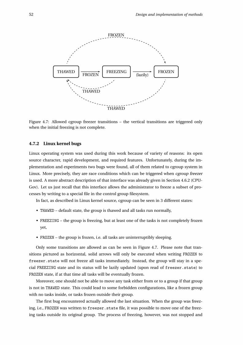
52 Design and implementation of methods
THAWED FREEZING FROZENFROZEN (lazily)
THAWED
THAWED
FROZEN
Figure 4.7: Allowed cgroup freezer transitions – the vertical transitions are triggered onlywhen the initial freezing is not complete.
4.7.2 Linux kernel bugs
Linux operating system was used during this work because of variety of reasons: its open
source character, rapid development, and required features. Unfortunately, during the im-
plementation and experiments two bugs were found, all of them related to cgroup system in
Linux. More precisely, they are race conditions which can be triggered when cgroup freezer
is used. A more abstract description of that interface was already given in Section 4.6.2 (CPU-
Gov). Let us just recall that this interface allows the administrator to freeze a subset of pro-
cesses by writing to a special file in the control group filesystem.
In fact, as described in Linux kernel source, cgroup can be seen in 3 different states:
• THAWED – default state, the group is thawed and all tasks run normally,
• FREEZING – the group is freezing, but at least one of the tasks is not completely frozen
yet,
• FROZEN – the group is frozen, i.e. all tasks are uninterruptibly sleeping.
Only some transitions are allowed as can be seen in Figure 4.7. Please note that tran-
sitions pictured as horizontal, solid arrows will only be executed when writing FROZEN to
freezer.state will not freeze all tasks immediately. Instead, the group will stay in a spe-
cial FREEZING state and its status will be lazily updated (upon read of freezer.state) to
FROZEN state, if at that time all tasks will be eventually frozen.
Moreover, one should not be able to move any task either from or to a group if that group
is not in THAWED state. This could lead to some forbidden configurations, like a frozen group
with no tasks inside, or tasks frozen outside their group.
The first bug encountered actually allowed the last situation. When the group was freez-
ing, i.e., FROZEN was written to freezer.state file, it was possible to move one of the freez-
ing tasks outside its original group. The process of freezing, however, was not stopped and
4.7. Problems encountered 53
the task could enter uninterruptible sleep outside its group. The effect is permanent – the
task cannot be thawed and will occupy system resources until the system is restarted. A min-
imal pseudocode snippet to trigger this bug is presented on the following listing (assuming
that cgroup freezer is mounted at /cg):
pid = fork ( ) ;
while ( ! pid ) {
/ * i n f i n i t e loop f o r a child * /
}
mkdir ( " /cg/ freeze_zone " ) ; / * c r e a t e a group * /
write ( " /cg/ freeze_zone / tasks " , s t r ( pid ) ) ; / * move the child there * /
write ( " /cg/ freeze_zone / fr ee ze r . s t a t e " , "FROZEN" ) ; / * f r e e z e the group * /
write ( " /cg/ tasks " , s t r ( pid ) ) ; / * move the child outside * /
The last operation should fail, but instead it is successful, ultimately blocking process
identified by pid forever.
A solution is to forbid migration of tasks between groups that are not thawed. This kind
of behavior was later implemented as a patch to the Linux kernel and successfully accepted
by developers.
Nevertheless, that is not the end of the story and after some time another bug was found.
The buggy implementation allowed a transition FREEZING → THAWED without any explicit ac-
tion of the user. It was enough to read freezer.state file fast enough to force this transition,
but, as is shown in Figure 4.7, one has to write THAWED value to do it. The transition would be
fired when none of the tasks from this group would be frozen yet, leading the kernel to the
conclusion that it is actually thawed. The processes, however, would become frozen anyway.
Additionally, the kernel implementation used a somewhat relaxed notion of frozen group.
It was possible to see a group in FROZEN state, but some of the tasks could be still running.
There are many ways to trigger this buggy behavior, but this one is particularly short:
pid = fork ( ) ;
while ( ! pid ) {
/ * i n f i n i t e loop f o r a child * /
}
mkdir ( " /cg/ freeze_zone " ) ; / * c r e a t e a group * /
write ( " /cg/ freeze_zone / tasks " , s t r ( pid ) ) ; / * move the child there * /
write ( " /cg/ freeze_zone / fr ee ze r . s t a t e " , "FROZEN" ) ; / * f r e e z e the group * /
read ( " /cg/ freeze_zone / fr ee ze r . s t a t e " , buf , 1 0 ) ; / * read the s t a t e * /
In the last line, the kernel updates the state of the group and, assuming that the task
identified by pid is not frozen yet, it will be incorrectly deduced that the group is thawed.
Fortunately, this situation can be reversed without rebooting – it suffices to freeze the group
again and thaw it.
A final solution for that was to rework the code a little bit:
• the state of the group can be changed lazily only from FREEZING state to FROZEN state,
• a more conservative definition of frozen task than before.
Again, a patch proposed by the authors was accepted by kernel developers. Table 4.1
summarizes the bugs found during the research. They should be released with the version
54 Design and implementation of methods
Commit message Commit ID
fix can_attach() to pro-hibit moving from/to freez-ing/frozen cgroups
2d3cbf8bc852ac1bc3d098186143c5973f87b753
update_freezer_state() does in-correct state transitions
0bdba580ab052a21e3eda2764ed22d9ee962392b
Table 4.1: Summary of the patches fixing discovered bugs.
2.6.37 of the Linux kernel.
4.7.3 Retrieving CPU configuration
As presented previously it is important for some methods to adjust to the hardware configu-
ration of the processors in the machine. Specifically, the CPU-Gov and CPU-Freq methods,
may profit from this information to aptly group virtual nodes that can switch their frequency
at the same time. That was already presented in Section 3.3.3.
It is therefore important to somehow gain the knowledge about the relations between pro-
cessors in the system. The first obvious way to do that is to use interface provided by CPU fre-
quency scaling subsystem as described in Section 4.5.1. The contents of files related_cpus
and affected_cpus should, if one believes in the documentation of the Linux kernel, con-
tain all necessary information. Unfortunately, to authors’ knowledge this information is in-
correct.
This observation was made during one of the tests. The results obtained by the CPU-
Gov method on one of the clusters were suspicious, because they were far away from the
expected behavior. Comparing this piece of information to the architecture returned by the
hwloc tool [BCOM+10], confusing inconsistency was found. For example, the following listing
shows how the Linux kernel returns the information on the CPU architecture of adonis cluster
node located in Grenoble, France:
cd / sys / devices /system/cpu/cpu0/ cpufreq /
cat related_cpus
0 2 3 4
On the other hand, the CPU architecture returned by hwloc is presented in Figure 4.8.
Clearly, these two pieces of information cannot be both correct – there is no obvious reason
why the frequency of the core 0 should be in any relation to the cores 2, 3, and 4, which are
located in a different socket.
Therefore the problem was reduced to finding out which source of information is correct
(if any): the one returned by the Linux kernel or the one given by hwloc tool. The experiment
to verify this claims consisted of the following steps:
1. Set all cores to the maximum frequency.
2. Run a CPU-intensive benchmark (see Section 5.2.1) and note the result.
3. Take any set of related cores (according to the tested source of information) and set the
cores’ frequency to the minimum value.
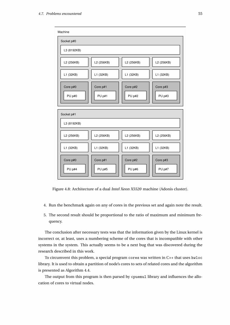
4.7. Problems encountered 55
Machine
Socket p#0
L3 (8192KB)
L2 (256KB)
L1 (32KB)
Core p#0
PU p#0
L2 (256KB)
L1 (32KB)
Core p#1
PU p#1
L2 (256KB)
L1 (32KB)
Core p#2
PU p#2
L2 (256KB)
L1 (32KB)
Core p#3
PU p#3
Socket p#1
L3 (8192KB)
L2 (256KB)
L1 (32KB)
Core p#0
PU p#4
L2 (256KB)
L1 (32KB)
Core p#1
PU p#5
L2 (256KB)
L1 (32KB)
Core p#2
PU p#6
L2 (256KB)
L1 (32KB)
Core p#3
PU p#7
Figure 4.8: Architecture of a dual Intel Xeon X5520 machine (Adonis cluster).
4. Run the benchmark again on any of cores in the previous set and again note the result.
5. The second result should be proportional to the ratio of maximum and minimum fre-
quency.
The conclusion after necessary tests was that the information given by the Linux kernel is
incorrect or, at least, uses a numbering scheme of the cores that is incompatible with other
systems in the system. This actually seems to be a next bug that was discovered during the
research described in this work.
To circumvent this problem, a special program cores was written in C++ that uses hwloc
library. It is used to obtain a partition of node’s cores to sets of related cores and the algorithm
is presented as Algorithm 4.4.
The output from this program is then parsed by cpuemul library and influences the allo-
cation of cores to virtual nodes.
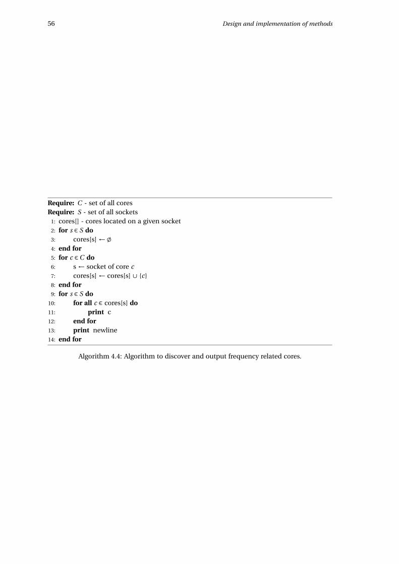
56 Design and implementation of methods
Require: C - set of all coresRequire: S - set of all sockets
1: cores[] - cores located on a given socket2: for s ∈ S do3: cores[s] ←;4: end for5: for c ∈C do6: s ← socket of core c7: cores[s] ← cores[s] ∪ {c}8: end for9: for s ∈ S do
10: for all c ∈ cores[s] do11: print c12: end for13: print newline14: end for
Algorithm 4.4: Algorithm to discover and output frequency related cores.
Chapter 5
Validation
In the following chapter the methods presented before are going to be evaluated. First, the
general idea how to do such a validation will be outlined. Then the benchmarks used during
the validation will be described. Next, a description of the so called large-scale experiment
will be given. Finally the results obtained will presented graphically, explained and conclu-
sions will be drawn.
5.1 Methodology
One of standard methods to evaluate an algorithm, a distributed system, or any solution
for a certain problem for that matter is to put it under a set of specific tests called micro-
benchmarks. They are devised and run to test the solution for a very specific and hermetic
conditions that focus only on one characteristic of the system. They are easy to design, easy
to understand and the expected output from their execution is usually easy to deduce before-
hand. A valid solution should necessarily pass them, so they serve as necessary conditions for
the validity of the method, or simply as unit tests known from software engineering. Notwith-
standing, micro-benchmarks are simulating unrealistic situations, detached from the normal
scenarios, and even satisfactory results obtained by means of micro-benchmarks will not im-
plicate that they will behave as good in the general case. Being aware of all advantages and
drawbacks of that approach, a set of micro-benchmarks was used in this work to validate the
presented methods.
The benchmarks test how the CPU emulation affects the following types of work:
• CPU-intensive work – represented for example by scientific computation,
• IO-intensive work – represented for example by network work, or by a typical interac-
tion of a human with the computer,
• both CPU and IO intensive work – almost every standard type of the work,
• multitasking work – inherent to multitasking operating systems and becoming much
more common nowadays with the advent of processors with multiple cores.
Also the memory speed is tested in CPU-emulated system.
57
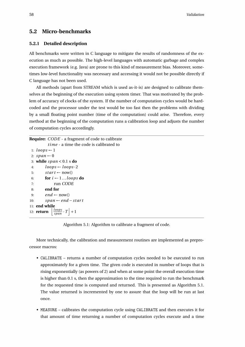
58 Validation
5.2 Micro-benchmarks
5.2.1 Detailed description
All benchmarks were written in C language to mitigate the results of randomness of the ex-
ecution as much as possible. The high-level languages with automatic garbage and complex
execution framework (e.g. Java) are prone to this kind of measurement bias. Moreover, some-
times low-level functionality was necessary and accessing it would not be possible directly if
C language has not been used.
All methods (apart from STREAM which is used as-it-is) are designed to calibrate them-
selves at the beginning of the execution using system timer. That was motivated by the prob-
lem of accuracy of clocks of the system. If the number of computation cycles would be hard-
coded and the processor under the test would be too fast then the problems with dividing
by a small floating point number (time of the computation) could arise. Therefore, every
method at the beginning of the computation runs a calibration loop and adjusts the number
of computation cycles accordingly.
Require: CODE - a fragment of code to calibrateRequire: t i me - a time the code is calibrated to
1: loops ← 12: span ← 03: while span < 0.1 s do4: loops ← l oops ·25: st ar t ← now()6: for i ← 1. . . loops do7: run CODE8: end for9: end ← now()
10: span ← end − st ar t11: end while12: return
⌊loopsspan ·T
⌋+1
Algorithm 5.1: Algorithm to calibrate a fragment of code.
More technically, the calibration and measurement routines are implemented as prepro-
cessor macros:
• CALIBRATE – returns a number of computation cycles needed to be executed to run
approximately for a given time. The given code is executed in number of loops that is
rising exponentially (as powers of 2) and when at some point the overall execution time
is higher than 0.1 s, then the approximation to the time required to run the benchmark
for the requested time is computed and returned. This is presented as Algorithm 5.1.
The value returned is incremented by one to assure that the loop will be run at last
once.
• MEASURE – calibrates the computation cycle using CALIBRATE and then executes it for
that amount of time returning a number of computation cycles execute and a time
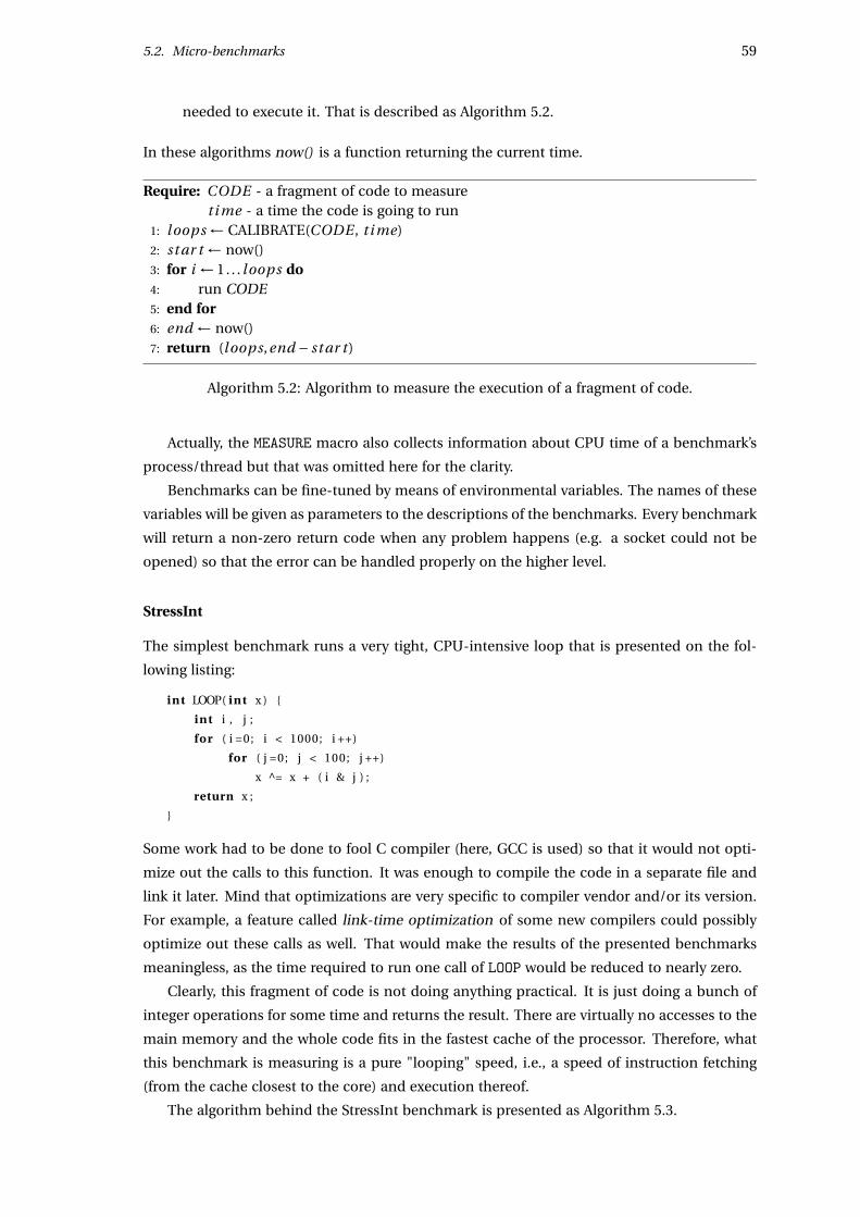
5.2. Micro-benchmarks 59
needed to execute it. That is described as Algorithm 5.2.
In these algorithms now() is a function returning the current time.
Require: CODE - a fragment of code to measureRequire: t i me - a time the code is going to run
1: loops ← CALIBRATE(CODE , t i me)2: st ar t ← now()3: for i ← 1. . . loops do4: run CODE5: end for6: end ← now()7: return (loops,end − st ar t )
Algorithm 5.2: Algorithm to measure the execution of a fragment of code.
Actually, the MEASURE macro also collects information about CPU time of a benchmark’s
process/thread but that was omitted here for the clarity.
Benchmarks can be fine-tuned by means of environmental variables. The names of these
variables will be given as parameters to the descriptions of the benchmarks. Every benchmark
will return a non-zero return code when any problem happens (e.g. a socket could not be
opened) so that the error can be handled properly on the higher level.
StressInt
The simplest benchmark runs a very tight, CPU-intensive loop that is presented on the fol-
lowing listing:
int LOOP( int x ) {
int i , j ;
for ( i =0; i < 1000; i ++)
for ( j =0; j < 100; j ++)
x ^= x + ( i & j ) ;
return x ;
}
Some work had to be done to fool C compiler (here, GCC is used) so that it would not opti-
mize out the calls to this function. It was enough to compile the code in a separate file and
link it later. Mind that optimizations are very specific to compiler vendor and/or its version.
For example, a feature called link-time optimization of some new compilers could possibly
optimize out these calls as well. That would make the results of the presented benchmarks
meaningless, as the time required to run one call of LOOP would be reduced to nearly zero.
Clearly, this fragment of code is not doing anything practical. It is just doing a bunch of
integer operations for some time and returns the result. There are virtually no accesses to the
main memory and the whole code fits in the fastest cache of the processor. Therefore, what
this benchmark is measuring is a pure "looping" speed, i.e., a speed of instruction fetching
(from the cache closest to the core) and execution thereof.
The algorithm behind the StressInt benchmark is presented as Algorithm 5.3.
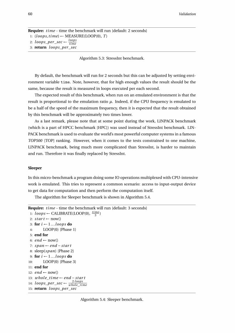
60 Validation
Require: t i me - time the benchmark will run {default: 2 seconds}1: (l oops, t i me) ← MEASURE(LOOP(0), T )
2: loops_per _sec ← loopsti me
3: return loops_per _sec
Algorithm 5.3: StressInt benchmark.
By default, the benchmark will run for 2 seconds but this can be adjusted by setting envi-
ronment variable time. Note, however, that for high enough values the result should be the
same, because the result is measured in loops executed per each second.
The expected result of this benchmark, when run on an emulated environment is that the
result is proportional to the emulation ratio µ. Indeed, if the CPU frequency is emulated to
be a half of the speed of the maximum frequency, then it is expected that the result obtained
by this benchmark will be approximately two times lower.
As a last remark, please note that at some point during the work, LINPACK benchmark
(which is a part of HPCC benchmark [HPC]) was used instead of StressInt benchmark. LIN-
PACK benchmark is used to evaluate the world’s most powerful computer systems in a famous
TOP500 [TOP] ranking. However, when it comes to the tests constrained to one machine,
LINPACK benchmark, being much more complicated than StressInt, is harder to maintain
and run. Therefore it was finally replaced by StressInt.
Sleeper
In this micro-benchmark a program doing some IO operations multiplexed with CPU-intensive
work is emulated. This tries to represent a common scenario: access to input-output device
to get data for computation and then perform the computation itself.
The algorithm for Sleeper benchmark is shown in Algorithm 5.4.
Require: t i me - time the benchmark will run {default: 3 seconds}1: loops ← CALIBRATE(LOOP(0), t i me
3 )2: st ar t ← now()3: for i ← 1. . . loops do4: LOOP(0) {Phase 1}5: end for6: end ← now()7: span ← end − st ar t8: sleep(span) {Phase 2}9: for i ← 1. . . loops do
10: LOOP(0) {Phase 3}11: end for12: end ← now()13: whole_t i me ← end − st ar t14: loops_per _sec ← 2·loops
whole_t i me15: return loops_per _sec
Algorithm 5.4: Sleeper benchmark.
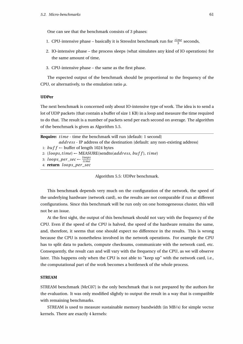
5.2. Micro-benchmarks 61
One can see that the benchmark consists of 3 phases:
1. CPU-intensive phase – basically it is StressInt benchmark run for t i me3 seconds,
2. IO-intensive phase – the process sleeps (what simulates any kind of IO operations) for
the same amount of time,
3. CPU-intensive phase – the same as the first phase.
The expected output of the benchmark should be proportional to the frequency of the
CPU, or alternatively, to the emulation ratio µ.
UDPer
The next benchmark is concerned only about IO-intensive type of work. The idea is to send a
lot of UDP packets (that contain a buffer of size 1 KB) in a loop and measure the time required
to do that. The result is a number of packets send per each second on average. The algorithm
of the benchmark is given as Algorithm 5.5.
Require: t i me - time the benchmark will run {default: 1 second}Require: addr ess - IP address of the destination {default: any non-existing address}
1: bu f f ← buffer of length 1024 bytes2: (loops, t i me) ← MEASURE(sendto(addr ess, bu f f ), t i me)
3: loops_per _sec ← loopsti me
4: return loops_per _sec
Algorithm 5.5: UDPer benchmark.
This benchmark depends very much on the configuration of the network, the speed of
the underlying hardware (network card), so the results are not comparable if run at different
configurations. Since this benchmark will be run only on one homogeneous cluster, this will
not be an issue.
At the first sight, the output of this benchmark should not vary with the frequency of the
CPU. Even if the speed of the CPU is halved, the speed of the hardware remains the same,
and, therefore, it seems that one should expect no difference in the results. This is wrong
because the CPU is nonetheless involved in the network operations. For example the CPU
has to split data to packets, compute checksums, communicate with the network card, etc.
Consequently, the result can and will vary with the frequency of the CPU, as we will observe
later. This happens only when the CPU is not able to "keep up" with the network card, i.e.,
the computational part of the work becomes a bottleneck of the whole process.
STREAM
STREAM benchmark [McC07] is the only benchmark that is not prepared by the authors for
the evaluation. It was only modified slightly to output the result in a way that is compatible
with remaining benchmarks.
STREAM is used to measure sustainable memory bandwidth (in MB/s) for simple vector
kernels. There are exactly 4 kernels:
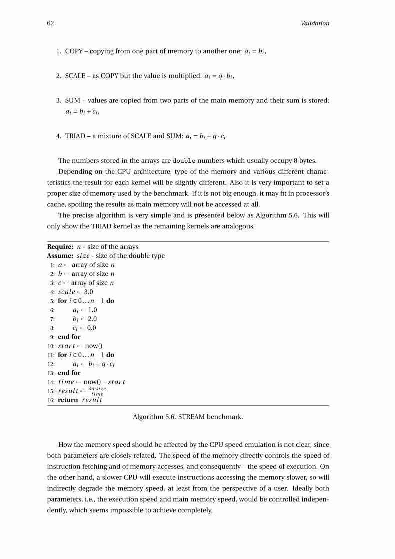
62 Validation
1. COPY – copying from one part of memory to another one: ai = bi ,
2. SCALE – as COPY but the value is multiplied: ai = q ·bi ,
3. SUM – values are copied from two parts of the main memory and their sum is stored:
ai = bi + ci ,
4. TRIAD – a mixture of SCALE and SUM: ai = bi +q · ci .
The numbers stored in the arrays are double numbers which usually occupy 8 bytes.
Depending on the CPU architecture, type of the memory and various different charac-
teristics the result for each kernel will be slightly different. Also it is very important to set a
proper size of memory used by the benchmark. If it is not big enough, it may fit in processor’s
cache, spoiling the results as main memory will not be accessed at all.
The precise algorithm is very simple and is presented below as Algorithm 5.6. This will
only show the TRIAD kernel as the remaining kernels are analogous.
Require: n - size of the arraysAssume: si ze - size of the double type
1: a ← array of size n2: b ← array of size n3: c ← array of size n4: scale ← 3.05: for i ∈ 0. . .n −1 do6: ai ← 1.07: bi ← 2.08: ci ← 0.09: end for
10: st ar t ← now()11: for i ∈ 0. . .n −1 do12: ai ← bi +q · ci
13: end for14: t i me ← now() −st ar t15: r esul t ← 3n·si ze
t i me16: return r esul t
Algorithm 5.6: STREAM benchmark.
How the memory speed should be affected by the CPU speed emulation is not clear, since
both parameters are closely related. The speed of the memory directly controls the speed of
instruction fetching and of memory accesses, and consequently – the speed of execution. On
the other hand, a slower CPU will execute instructions accessing the memory slower, so will
indirectly degrade the memory speed, at least from the perspective of a user. Ideally both
parameters, i.e., the execution speed and main memory speed, would be controlled indepen-
dently, which seems impossible to achieve completely.
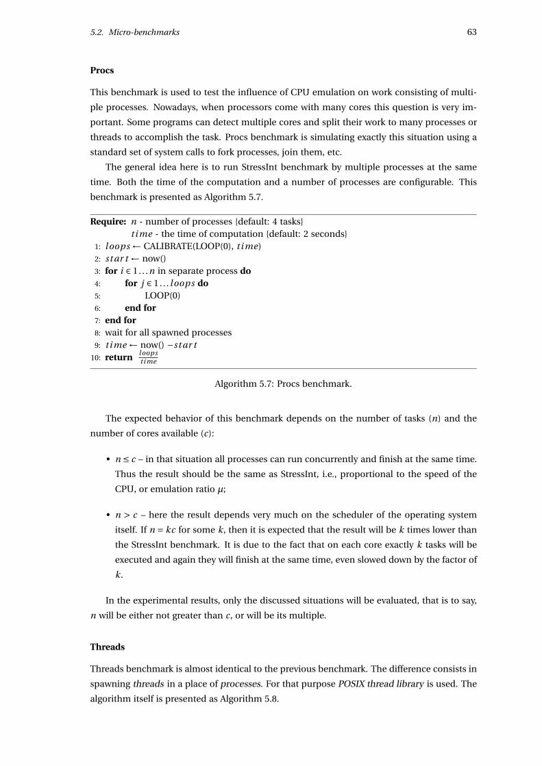
5.2. Micro-benchmarks 63
Procs
This benchmark is used to test the influence of CPU emulation on work consisting of multi-
ple processes. Nowadays, when processors come with many cores this question is very im-
portant. Some programs can detect multiple cores and split their work to many processes or
threads to accomplish the task. Procs benchmark is simulating exactly this situation using a
standard set of system calls to fork processes, join them, etc.
The general idea here is to run StressInt benchmark by multiple processes at the same
time. Both the time of the computation and a number of processes are configurable. This
benchmark is presented as Algorithm 5.7.
Require: n - number of processes {default: 4 tasks}Require: t i me - the time of computation {default: 2 seconds}
1: loops ← CALIBRATE(LOOP(0), t i me)2: st ar t ← now()3: for i ∈ 1. . .n in separate process do4: for j ∈ 1. . . loops do5: LOOP(0)6: end for7: end for8: wait for all spawned processes9: t i me ← now() −st ar t
10: return loopsti me
Algorithm 5.7: Procs benchmark.
The expected behavior of this benchmark depends on the number of tasks (n) and the
number of cores available (c):
• n ≤ c – in that situation all processes can run concurrently and finish at the same time.
Thus the result should be the same as StressInt, i.e., proportional to the speed of the
CPU, or emulation ratio µ;
• n > c – here the result depends very much on the scheduler of the operating system
itself. If n = kc for some k, then it is expected that the result will be k times lower than
the StressInt benchmark. It is due to the fact that on each core exactly k tasks will be
executed and again they will finish at the same time, even slowed down by the factor of
k.
In the experimental results, only the discussed situations will be evaluated, that is to say,
n will be either not greater than c, or will be its multiple.
Threads
Threads benchmark is almost identical to the previous benchmark. The difference consists in
spawning threads in a place of processes. For that purpose POSIX thread library is used. The
algorithm itself is presented as Algorithm 5.8.
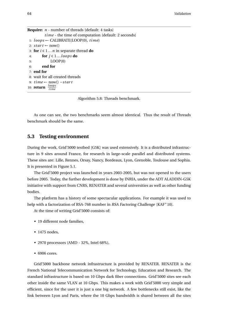
64 Validation
Require: n - number of threads {default: 4 tasks}Require: t i me - the time of computation {default: 2 seconds}
1: loops ← CALIBRATE(LOOP(0), t i me)2: st ar t ← now()3: for i ∈ 1. . .n in separate thread do4: for j ∈ 1. . . loops do5: LOOP(0)6: end for7: end for8: wait for all created threads9: t i me ← now() −st ar t
10: return l oopsti me
Algorithm 5.8: Threads benchmark.
As one can see, the two benchmarks seem almost identical. Thus the result of Threads
benchmark should be the same.
5.3 Testing environment
During the work, Grid’5000 testbed [G5K] was used extensively. It is a distributed infrastruc-
ture in 9 sites around France, for research in large-scale parallel and distributed systems.
These sites are: Lille, Rennes, Orsay, Nancy, Bordeaux, Lyon, Grenoble, Toulouse and Sophia.
It is presented in Figure 5.1.
The Grid’5000 project was launched in years 2003-2005, but was not opened to the users
before 2005. Today, the further development is done by INRIA, under the ADT ALADDIN-G5K
initiative with support from CNRS, RENATER and several universities as well as other funding
bodies.
The platform has a history of some spectacular applications. For example it was used to
help with a factorization of RSA-768 number in RSA Factoring Challenge [KAF+10].
At the time of writing Grid’5000 consists of:
• 19 different node families,
• 1475 nodes,
• 2970 processors (AMD - 32%, Intel 68%),
• 6906 cores.
Grid’5000 backbone network infrastructure is provided by RENATER. RENATER is the
French National Telecommunication Network for Technology, Education and Research. The
standard infrastructure is based on 10 Gbps dark fiber connections. Grid’5000 sites see each
other inside the same VLAN at 10 Gbps. This makes a work with Grid’5000 very simple and
efficient, since for the user it is just a one big network. A few bottlenecks still exist, like the
link between Lyon and Paris, where the 10 Gbps bandwidth is shared between all the sites
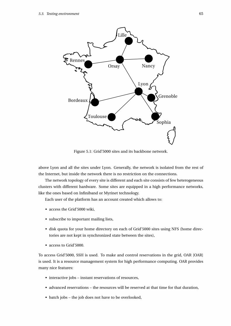
5.3. Testing environment 65
Bordeaux
Rennes
SophiaToulouse
Orsay
Lille
Nancy
Lyon
Grenoble
Figure 5.1: Grid’5000 sites and its backbone network.
above Lyon and all the sites under Lyon. Generally, the network is isolated from the rest of
the Internet, but inside the network there is no restriction on the connections.
The network topology of every site is different and each site consists of few heterogeneous
clusters with different hardware. Some sites are equipped in a high performance networks,
like the ones based on Infiniband or Myrinet technology.
Each user of the platform has an account created which allows to:
• access the Grid’5000 wiki,
• subscribe to important mailing lists,
• disk quota for your home directory on each of Grid’5000 sites using NFS (home direc-
tories are not kept in synchronized state between the sites),
• access to Grid’5000.
To access Grid’5000, SSH is used. To make and control reservations in the grid, OAR [OAR]
is used. It is a resource management system for high performance computing. OAR provides
many nice features:
• interactive jobs – instant reservations of resources,
• advanced reservations – the resources will be reserved at that time for that duration,
• batch jobs – the job does not have to be overlooked,
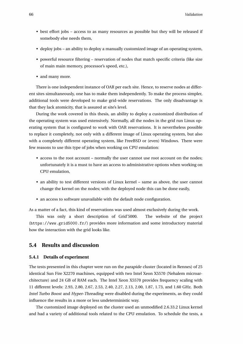
66 Validation
• best effort jobs – access to as many resources as possible but they will be released if
somebody else needs them,
• deploy jobs – an ability to deploy a manually customized image of an operating system,
• powerful resource filtering – reservation of nodes that match specific criteria (like size
of main main memory, processor’s speed, etc.),
• and many more.
There is one independent instance of OAR per each site. Hence, to reserve nodes at differ-
ent sites simultaneously, one has to make them independently. To make the process simpler,
additional tools were developed to make grid-wide reservations. The only disadvantage is
that they lack atomicity, that is assured at site’s level.
During the work covered in this thesis, an ability to deploy a customized distribution of
the operating system was used extensively. Normally, all the nodes in the grid run Linux op-
erating system that is configured to work with OAR reservations. It is nevertheless possible
to replace it completely, not only with a different image of Linux operating system, but also
with a completely different operating system, like FreeBSD or (even) Windows. There were
few reasons to use this type of jobs when working on CPU emulation:
• access to the root account – normally the user cannot use root account on the nodes;
unfortunately it is a must to have an access to administrative options when working on
CPU emulation,
• an ability to test different versions of Linux kernel – same as above, the user cannot
change the kernel on the nodes; with the deployed node this can be done easily,
• an access to software unavailable with the default node configuration.
As a matter of a fact, this kind of reservations was used almost exclusively during the work.
This was only a short description of Grid’5000. The website of the project
(https://www.grid5000.fr/) provides more information and some introductory material
how the interaction with the grid looks like.
5.4 Results and discussion
5.4.1 Details of experiment
The tests presented in this chapter were run on the parapide cluster (located in Rennes) of 25
identical Sun Fire X2270 machines, equipped with two Intel Xeon X5570 (Nehalem microar-
chitecture) and 24 GB of RAM each. The Intel Xeon X5570 provides frequency scaling with
11 different levels: 2.93, 2.80, 2.67, 2.53, 2.40, 2.27, 2.13, 2.00, 1.87, 1.73, and 1.60 GHz. Both
Intel Turbo Boost and Hyper-Threading were disabled during the experiments, as they could
influence the results in a more or less undeterministic way.
The customized image deployed on the cluster used an unmodified 2.6.33.2 Linux kernel
and had a variety of additional tools related to the CPU emulation. To schedule the tests, a
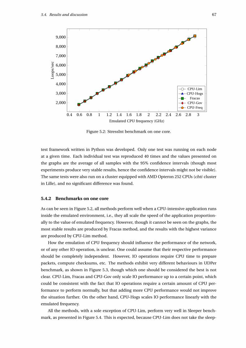
5.4. Results and discussion 67
0.4 0.6 0.8 1 1.2 1.4 1.6 1.8 2 2.2 2.4 2.6 2.8 3
2,000
3,000
4,000
5,000
6,000
7,000
8,000
9,000
Emulated CPU frequency (GHz)
Loo
ps/
sec
CPU-LimCPU-Hogs
FracasCPU-GovCPU-Freq
Figure 5.2: StressInt benchmark on one core.
test framework written in Python was developed. Only one test was running on each node
at a given time. Each individual test was reproduced 40 times and the values presented on
the graphs are the average of all samples with the 95% confidence intervals (though most
experiments produce very stable results, hence the confidence intervals might not be visible).
The same tests were also run on a cluster equipped with AMD Opteron 252 CPUs (chti cluster
in Lille), and no significant difference was found.
5.4.2 Benchmarks on one core
As can be seen in Figure 5.2, all methods perform well when a CPU-intensive application runs
inside the emulated environment, i.e., they all scale the speed of the application proportion-
ally to the value of emulated frequency. However, though it cannot be seen on the graphs, the
most stable results are produced by Fracas method, and the results with the highest variance
are produced by CPU-Lim method.
How the emulation of CPU frequency should influence the performance of the network,
or of any other IO operation, is unclear. One could assume that their respective performance
should be completely independent. However, IO operations require CPU time to prepare
packets, compute checksums, etc. The methods exhibit very different behaviours in UDPer
benchmark, as shown in Figure 5.3, though which one should be considered the best is not
clear. CPU-Lim, Fracas and CPU-Gov only scale IO performance up to a certain point, which
could be consistent with the fact that IO operations require a certain amount of CPU per-
formance to perform normally, but that adding more CPU performance would not improve
the situation further. On the other hand, CPU-Hogs scales IO performance linearly with the
emulated frequency.
All the methods, with a sole exception of CPU-Lim, perform very well in Sleeper bench-
mark, as presented in Figure 5.4. This is expected, because CPU-Lim does not take the sleep-
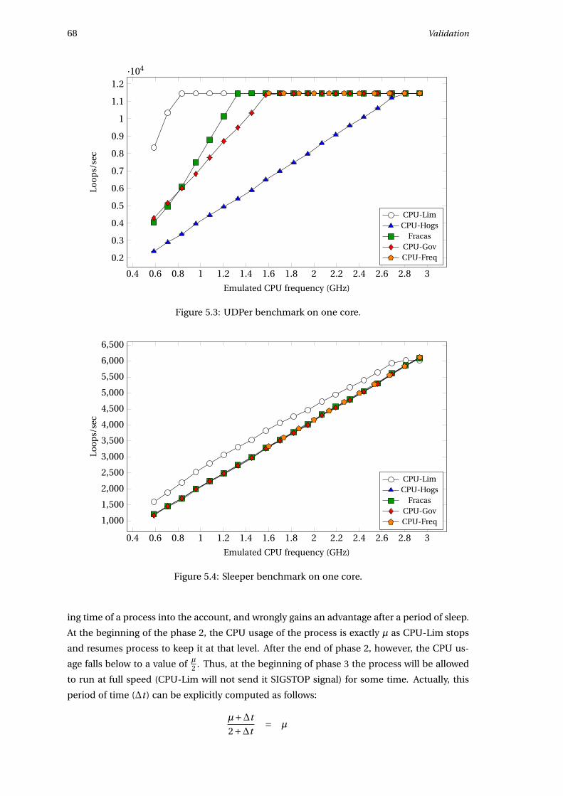
68 Validation
0.4 0.6 0.8 1 1.2 1.4 1.6 1.8 2 2.2 2.4 2.6 2.8 3
0.2
0.3
0.4
0.5
0.6
0.7
0.8
0.9
1
1.1
1.2·104
Emulated CPU frequency (GHz)
Loo
ps/
sec
CPU-LimCPU-Hogs
FracasCPU-GovCPU-Freq
Figure 5.3: UDPer benchmark on one core.
0.4 0.6 0.8 1 1.2 1.4 1.6 1.8 2 2.2 2.4 2.6 2.8 3
1,000
1,500
2,000
2,500
3,000
3,500
4,000
4,500
5,000
5,500
6,000
6,500
Emulated CPU frequency (GHz)
Loo
ps/
sec
CPU-LimCPU-Hogs
FracasCPU-GovCPU-Freq
Figure 5.4: Sleeper benchmark on one core.
ing time of a process into the account, and wrongly gains an advantage after a period of sleep.
At the beginning of the phase 2, the CPU usage of the process is exactly µ as CPU-Lim stops
and resumes process to keep it at that level. After the end of phase 2, however, the CPU us-
age falls below to a value of µ2 . Thus, at the beginning of phase 3 the process will be allowed
to run at full speed (CPU-Lim will not send it SIGSTOP signal) for some time. Actually, this
period of time (∆t ) can be explicitly computed as follows:
µ+∆t
2+∆t= µ
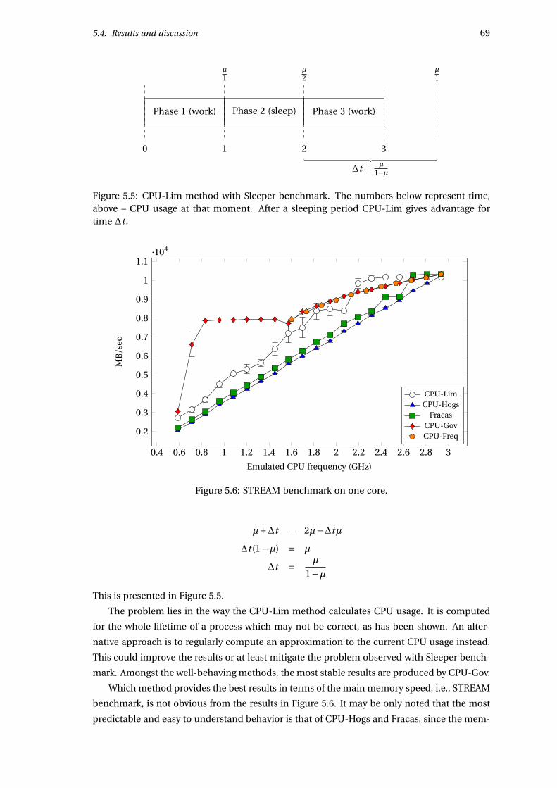
5.4. Results and discussion 69
Phase 1 (work) Phase 2 (sleep) Phase 3 (work)
0 1 2 3
µ1
µ2
µ1
∆t = µ1−µ
Figure 5.5: CPU-Lim method with Sleeper benchmark. The numbers below represent time,above – CPU usage at that moment. After a sleeping period CPU-Lim gives advantage fortime ∆t .
0.4 0.6 0.8 1 1.2 1.4 1.6 1.8 2 2.2 2.4 2.6 2.8 3
0.2
0.3
0.4
0.5
0.6
0.7
0.8
0.9
1
1.1·104
Emulated CPU frequency (GHz)
MB
/sec
CPU-LimCPU-Hogs
FracasCPU-GovCPU-Freq
Figure 5.6: STREAM benchmark on one core.
µ+∆t = 2µ+∆tµ
∆t (1−µ) = µ
∆t = µ
1−µ
This is presented in Figure 5.5.
The problem lies in the way the CPU-Lim method calculates CPU usage. It is computed
for the whole lifetime of a process which may not be correct, as has been shown. An alter-
native approach is to regularly compute an approximation to the current CPU usage instead.
This could improve the results or at least mitigate the problem observed with Sleeper bench-
mark. Amongst the well-behaving methods, the most stable results are produced by CPU-Gov.
Which method provides the best results in terms of the main memory speed, i.e., STREAM
benchmark, is not obvious from the results in Figure 5.6. It may be only noted that the most
predictable and easy to understand behavior is that of CPU-Hogs and Fracas, since the mem-
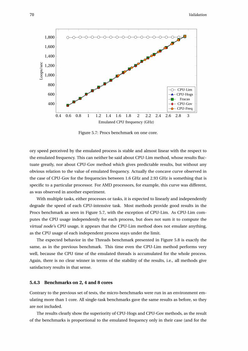
70 Validation
0.4 0.6 0.8 1 1.2 1.4 1.6 1.8 2 2.2 2.4 2.6 2.8 3
400
600
800
1,000
1,200
1,400
1,600
1,800
Emulated CPU frequency (GHz)
Loo
ps/
sec
CPU-LimCPU-Hogs
FracasCPU-GovCPU-Freq
Figure 5.7: Procs benchmark on one core.
ory speed perceived by the emulated process is stable and almost linear with the respect to
the emulated frequency. This can neither be said about CPU-Lim method, whose results fluc-
tuate greatly, nor about CPU-Gov method which gives predictable results, but without any
obvious relation to the value of emulated frequency. Actually the concave curve observed in
the case of CPU-Gov for the frequencies between 1.6 GHz and 2.93 GHz is something that is
specific to a particular processor. For AMD processors, for example, this curve was different,
as was observed in another experiment.
With multiple tasks, either processes or tasks, it is expected to linearly and independently
degrade the speed of each CPU-intensive task. Most methods provide good results in the
Procs benchmark as seen in Figure 5.7, with the exception of CPU-Lim. As CPU-Lim com-
putes the CPU usage independently for each process, but does not sum it to compute the
virtual node ’s CPU usage, it appears that the CPU-Lim method does not emulate anything,
as the CPU usage of each independent process stays under the limit.
The expected behavior in the Threads benchmark presented in Figure 5.8 is exactly the
same, as in the previous benchmark. This time even the CPU-Lim method performs very
well, because the CPU time of the emulated threads is accumulated for the whole process.
Again, there is no clear winner in terms of the stability of the results, i.e., all methods give
satisfactory results in that sense.
5.4.3 Benchmarks on 2, 4 and 8 cores
Contrary to the previous set of tests, the micro-benchmarks were run in an environment em-
ulating more than 1 core. All single-task benchmarks gave the same results as before, so they
are not included.
The results clearly show the superiority of CPU-Hogs and CPU-Gov methods, as the result
of the benchmarks is proportional to the emulated frequency only in their case (and for the
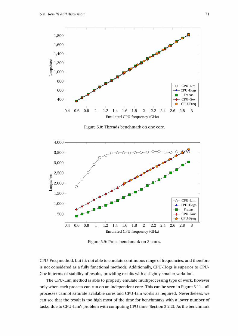
5.4. Results and discussion 71
0.4 0.6 0.8 1 1.2 1.4 1.6 1.8 2 2.2 2.4 2.6 2.8 3
400
600
800
1,000
1,200
1,400
1,600
1,800
Emulated CPU frequency (GHz)
Loo
ps/
sec
CPU-LimCPU-Hogs
FracasCPU-GovCPU-Freq
Figure 5.8: Threads benchmark on one core.
0.4 0.6 0.8 1 1.2 1.4 1.6 1.8 2 2.2 2.4 2.6 2.8 3
500
1,000
1,500
2,000
2,500
3,000
3,500
4,000
Emulated CPU frequency (GHz)
Loo
ps/
sec
CPU-LimCPU-Hogs
FracasCPU-GovCPU-Freq
Figure 5.9: Procs benchmark on 2 cores.
CPU-Freq method, but it’s not able to emulate continuous range of frequencies, and therefore
is not considered as a fully functional method). Additionally, CPU-Hogs is superior to CPU-
Gov in terms of stability of results, providing results with a slightly smaller variation.
The CPU-Lim method is able to properly emulate multiprocessing type of work, however
only when each process can run on an independent core. This can be seen in Figure 5.11 – all
processes cannot saturate available cores and CPU-Lim works as required. Nevertheless, we
can see that the result is too high most of the time for benchmarks with a lower number of
tasks, due to CPU-Lim’s problem with computing CPU time (Section 3.2.2). As the benchmark
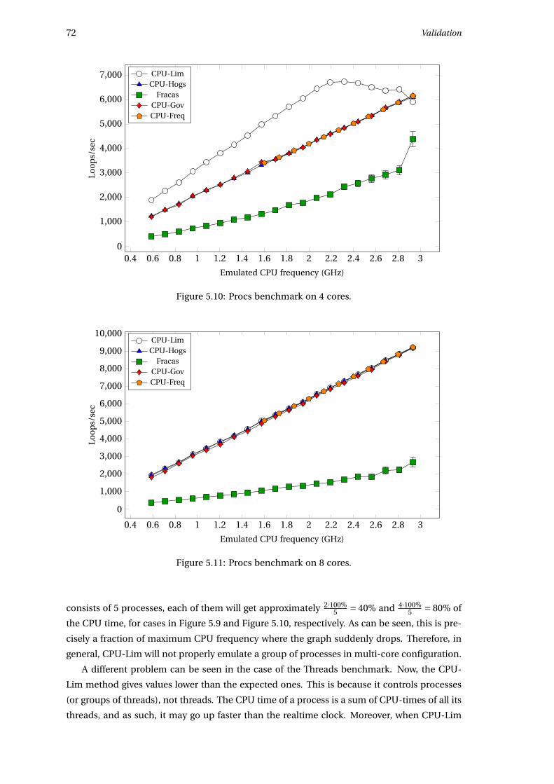
72 Validation
0.4 0.6 0.8 1 1.2 1.4 1.6 1.8 2 2.2 2.4 2.6 2.8 30
1,000
2,000
3,000
4,000
5,000
6,000
7,000
Emulated CPU frequency (GHz)
Loo
ps/
sec
CPU-LimCPU-Hogs
FracasCPU-GovCPU-Freq
Figure 5.10: Procs benchmark on 4 cores.
0.4 0.6 0.8 1 1.2 1.4 1.6 1.8 2 2.2 2.4 2.6 2.8 3
0
1,000
2,000
3,000
4,000
5,000
6,000
7,000
8,000
9,000
10,000
Emulated CPU frequency (GHz)
Loo
ps/
sec
CPU-LimCPU-Hogs
FracasCPU-GovCPU-Freq
Figure 5.11: Procs benchmark on 8 cores.
consists of 5 processes, each of them will get approximately 2·100%5 = 40% and 4·100%
5 = 80% of
the CPU time, for cases in Figure 5.9 and Figure 5.10, respectively. As can be seen, this is pre-
cisely a fraction of maximum CPU frequency where the graph suddenly drops. Therefore, in
general, CPU-Lim will not properly emulate a group of processes in multi-core configuration.
A different problem can be seen in the case of the Threads benchmark. Now, the CPU-
Lim method gives values lower than the expected ones. This is because it controls processes
(or groups of threads), not threads. The CPU time of a process is a sum of CPU-times of all its
threads, and as such, it may go up faster than the realtime clock. Moreover, when CPU-Lim
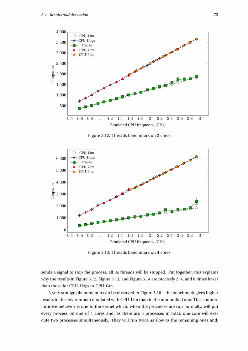
5.4. Results and discussion 73
0.4 0.6 0.8 1 1.2 1.4 1.6 1.8 2 2.2 2.4 2.6 2.8 3
500
1,000
1,500
2,000
2,500
3,000
3,500
4,000
Emulated CPU frequency (GHz)
Loo
ps/
sec
CPU-LimCPU-Hogs
FracasCPU-GovCPU-Freq
Figure 5.12: Threads benchmark on 2 cores.
0.4 0.6 0.8 1 1.2 1.4 1.6 1.8 2 2.2 2.4 2.6 2.8 30
1,000
2,000
3,000
4,000
5,000
6,000
Emulated CPU frequency (GHz)
Loo
ps/
sec
CPU-LimCPU-Hogs
FracasCPU-GovCPU-Freq
Figure 5.13: Threads benchmark on 4 cores.
sends a signal to stop the process, all its threads will be stopped. Put together, this explains
why the results in Figure 5.12, Figure 5.13, and Figure 5.14 are precisely 2, 4, and 8 times lower
than those for CPU-Hogs or CPU-Gov.
A very strange phenomenon can be observed in Figure 5.10 – the benchmark gives higher
results in the environment emulated with CPU-Lim than in the unmodified one. This counter-
intuitive behavior is due to the kernel which, when the processes are run normally, will put
every process on one of 4 cores and, as there are 5 processes in total, one core will exe-
cute two processes simultaneously. They will run twice as slow as the remaining ones and,
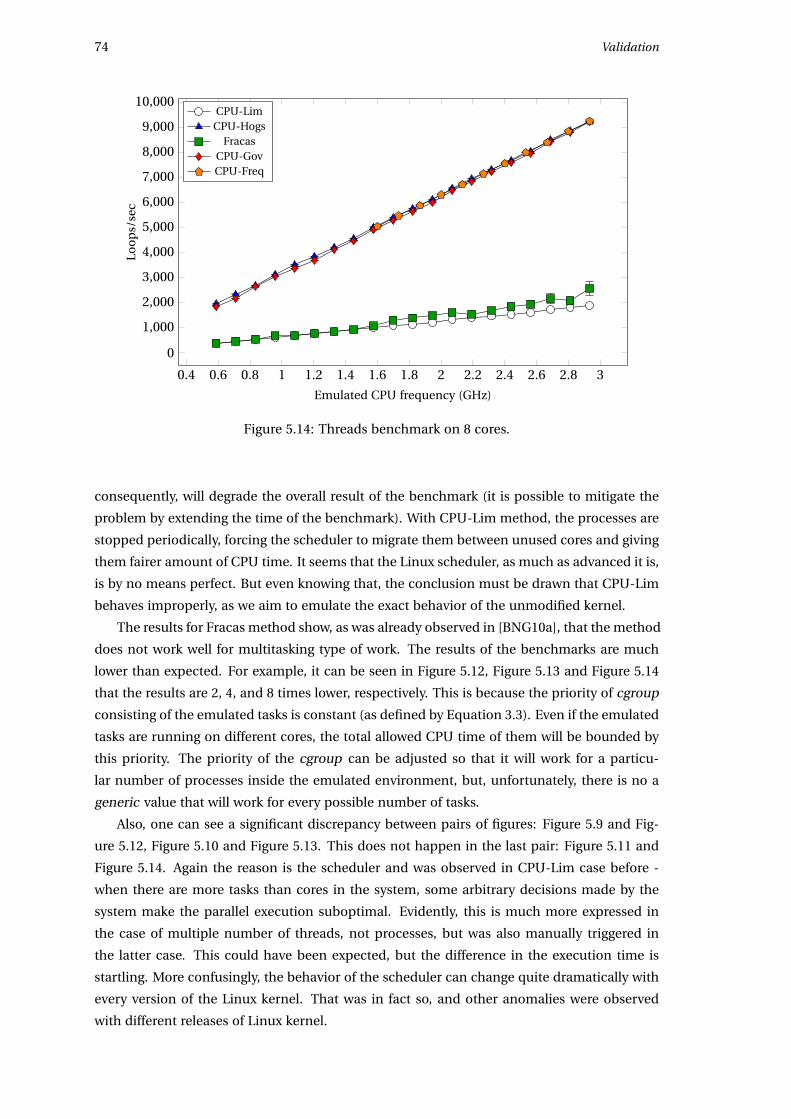
74 Validation
0.4 0.6 0.8 1 1.2 1.4 1.6 1.8 2 2.2 2.4 2.6 2.8 3
0
1,000
2,000
3,000
4,000
5,000
6,000
7,000
8,000
9,000
10,000
Emulated CPU frequency (GHz)
Loo
ps/
sec
CPU-LimCPU-Hogs
FracasCPU-GovCPU-Freq
Figure 5.14: Threads benchmark on 8 cores.
consequently, will degrade the overall result of the benchmark (it is possible to mitigate the
problem by extending the time of the benchmark). With CPU-Lim method, the processes are
stopped periodically, forcing the scheduler to migrate them between unused cores and giving
them fairer amount of CPU time. It seems that the Linux scheduler, as much as advanced it is,
is by no means perfect. But even knowing that, the conclusion must be drawn that CPU-Lim
behaves improperly, as we aim to emulate the exact behavior of the unmodified kernel.
The results for Fracas method show, as was already observed in [BNG10a], that the method
does not work well for multitasking type of work. The results of the benchmarks are much
lower than expected. For example, it can be seen in Figure 5.12, Figure 5.13 and Figure 5.14
that the results are 2, 4, and 8 times lower, respectively. This is because the priority of cgroup
consisting of the emulated tasks is constant (as defined by Equation 3.3). Even if the emulated
tasks are running on different cores, the total allowed CPU time of them will be bounded by
this priority. The priority of the cgroup can be adjusted so that it will work for a particu-
lar number of processes inside the emulated environment, but, unfortunately, there is no a
generic value that will work for every possible number of tasks.
Also, one can see a significant discrepancy between pairs of figures: Figure 5.9 and Fig-
ure 5.12, Figure 5.10 and Figure 5.13. This does not happen in the last pair: Figure 5.11 and
Figure 5.14. Again the reason is the scheduler and was observed in CPU-Lim case before -
when there are more tasks than cores in the system, some arbitrary decisions made by the
system make the parallel execution suboptimal. Evidently, this is much more expressed in
the case of multiple number of threads, not processes, but was also manually triggered in
the latter case. This could have been expected, but the difference in the execution time is
startling. More confusingly, the behavior of the scheduler can change quite dramatically with
every version of the Linux kernel. That was in fact so, and other anomalies were observed
with different releases of Linux kernel.
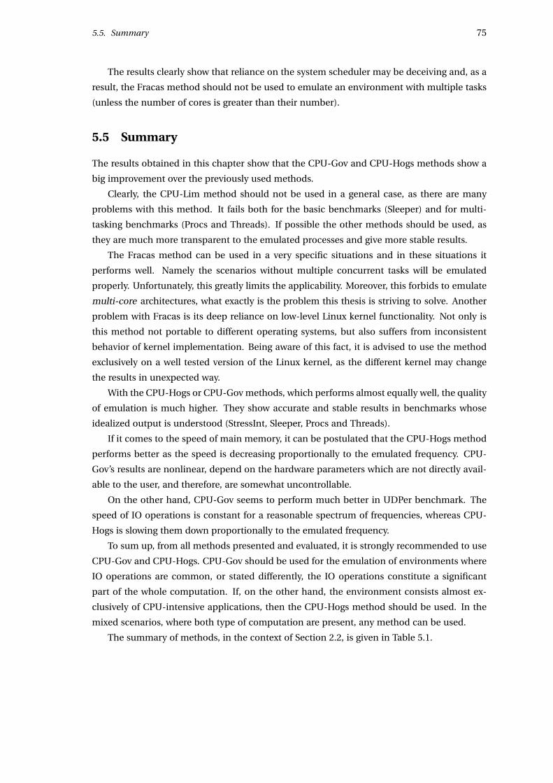
5.5. Summary 75
The results clearly show that reliance on the system scheduler may be deceiving and, as a
result, the Fracas method should not be used to emulate an environment with multiple tasks
(unless the number of cores is greater than their number).
5.5 Summary
The results obtained in this chapter show that the CPU-Gov and CPU-Hogs methods show a
big improvement over the previously used methods.
Clearly, the CPU-Lim method should not be used in a general case, as there are many
problems with this method. It fails both for the basic benchmarks (Sleeper) and for multi-
tasking benchmarks (Procs and Threads). If possible the other methods should be used, as
they are much more transparent to the emulated processes and give more stable results.
The Fracas method can be used in a very specific situations and in these situations it
performs well. Namely the scenarios without multiple concurrent tasks will be emulated
properly. Unfortunately, this greatly limits the applicability. Moreover, this forbids to emulate
multi-core architectures, what exactly is the problem this thesis is striving to solve. Another
problem with Fracas is its deep reliance on low-level Linux kernel functionality. Not only is
this method not portable to different operating systems, but also suffers from inconsistent
behavior of kernel implementation. Being aware of this fact, it is advised to use the method
exclusively on a well tested version of the Linux kernel, as the different kernel may change
the results in unexpected way.
With the CPU-Hogs or CPU-Gov methods, which performs almost equally well, the quality
of emulation is much higher. They show accurate and stable results in benchmarks whose
idealized output is understood (StressInt, Sleeper, Procs and Threads).
If it comes to the speed of main memory, it can be postulated that the CPU-Hogs method
performs better as the speed is decreasing proportionally to the emulated frequency. CPU-
Gov’s results are nonlinear, depend on the hardware parameters which are not directly avail-
able to the user, and therefore, are somewhat uncontrollable.
On the other hand, CPU-Gov seems to perform much better in UDPer benchmark. The
speed of IO operations is constant for a reasonable spectrum of frequencies, whereas CPU-
Hogs is slowing them down proportionally to the emulated frequency.
To sum up, from all methods presented and evaluated, it is strongly recommended to use
CPU-Gov and CPU-Hogs. CPU-Gov should be used for the emulation of environments where
IO operations are common, or stated differently, the IO operations constitute a significant
part of the whole computation. If, on the other hand, the environment consists almost ex-
clusively of CPU-intensive applications, then the CPU-Hogs method should be used. In the
mixed scenarios, where both type of computation are present, any method can be used.
The summary of methods, in the context of Section 2.2, is given in Table 5.1.
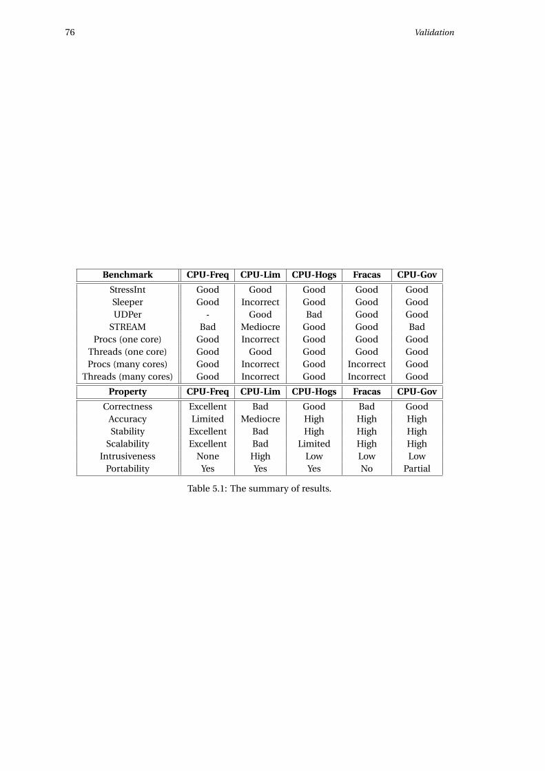
76 Validation
Benchmark CPU-Freq CPU-Lim CPU-Hogs Fracas CPU-Gov
StressInt Good Good Good Good GoodSleeper Good Incorrect Good Good GoodUDPer - Good Bad Good Good
STREAM Bad Mediocre Good Good BadProcs (one core) Good Incorrect Good Good Good
Threads (one core) Good Good Good Good GoodProcs (many cores) Good Incorrect Good Incorrect Good
Threads (many cores) Good Incorrect Good Incorrect Good
Property CPU-Freq CPU-Lim CPU-Hogs Fracas CPU-Gov
Correctness Excellent Bad Good Bad GoodAccuracy Limited Mediocre High High HighStability Excellent Bad High High High
Scalability Excellent Bad Limited High HighIntrusiveness None High Low Low Low
Portability Yes Yes Yes No Partial
Table 5.1: The summary of results.
Chapter 6
Conclusions
6.1 Summary of the work
This work is an effort to cope with the problem of reproducibility of the results scientific re-
sults in computer science. Every scientific result should verifiable, as happens normally in
publications on mathematics, for example. The difficulty of reproducing the experimental
results is a problem that haunts computer science community, as sometimes the results pre-
sented in papers cannot be reproduced by the readers, and sometimes even by the authors
themselves. There is no obvious solution to this, but with CPU emulation and other tech-
niques used together, at least the conditions of the environment can be controlled determin-
istically and reproduced if needed.
Moreover, the multi-core emulation of processors can be used to run experiments that
normally would not be attainable. The idea is to exploit the fact that machines with multiple
processors and cores can be used to emulate multiple machines, effectively enlarging the
scale of the experiments by an order of magnitude with the same hardware.
Additionally, the emulation of CPU performance is an important asset in the context
of the evaluation of applications targeted at heterogeneous systems. In this thesis, existing
methods for this problem were presented: CPU-Freq, CPU-Lim, CPU-Burn and Fracas. All
these methods have been thoroughly described and their advantages and disadvantages have
been explained. As a result the necessity of devising new methods for this particular problem
was established, as no method was satisfactory. Consequently, new methods were devised
and are proposed in this work: CPU-Gov and CPU-Hogs. The CPU-Gov method is a clever
generalization of CPU-Freq method, and the CPU-Hogs method is a multi-core implementa-
tion of the CPU burning technique.
The thesis contains many theoretical definitions in the domain of multi-core emulation
of CPU performance. To authors’ knowledge it happens to be the most complete discourse
on the subject so far.
After description of both the idea and the implementation of all methods, they were eval-
uated to compare their applicability and quality. The validation used a set of carefully pre-
pared micro-benchmarks testing the most important features of the methods. It was shown
very precisely that the existing methods cannot emulate the general case of CPU emulation
problem. On the other hand, the new methods perform exceedingly better in virtually ev-
77
78 Conclusions
ery situation and both can be used to emulate ever more complex scenarios. We believe that
these two methods are nearly optimal solutions to the problem of CPU emulation and can be
considered the current state-of-the-art knowledge in this domain.
6.2 Future work
First, a more complex validation of CPU emulation methods should be done than the one by
means of micro-benchmarks only. They give only a limited insight to the correctness of the
emulation as every one considers an artificial scenario.
Also, and this was an idea at the very beginning of the research, the methods presented
could be integrated in Wrekavoc, which is a tool to emulate complex network topologies with
fine-grained control over parameters of the nodes. Moreover, the methods could be ported to
other operating systems and evaluated there to see if the results are the same.
The emulation of memory speed should be investigated. This can be crucial in some
applications where the speed of main memory is a factor that cannot be neglected. This is
becoming more important as NUMA systems are becoming more popular.
The more complex emulation of processors could be considered. In this work we focus
on the speed of processors, but it would be interesting to control other features of it: size of
caches at different levels, simultaneous multithreading implementations in processors, etc.
This appears to be a very difficult problem, as these parameters of processor are of great
complexity, and very small periods of time are involved. It is even doubtful if this can be
controlled from the software at all.
Finally, some work could be done in the domain of reproducibility and scalability of ex-
periments. Distest framework is an interesting approach to achieve both of them.
Appendix A
Streszczenie
W pracy tej dyskutowane jest zagadnienie emulacji predkosci proceso-
rów wielordzeniowych. Poza przedstawieniem istniejacych rozwiazan
oraz aktualnego stanu wiedzy na ten temat, przedstawione sa dwa nowe
podejscia: CPU-Hogs oraz CPU-Gov, które w załozeniu maja usprawnic
jakosc emulacji. Po krótkim omówieniu metod oraz ich implementacji,
wszystkie one sa poddane testom, które pokazuja, ze nowe propozycje
sa rzeczywiscie lepsze. Praca zamyka sie podsumowaniem, w którym
przedstawiono koncowe wnioski z wyników badan oraz dalsze kierunki
badan.
Podczas prac wykryto w jadrze systemu operacyjnego Linux błedy, do
których poprawki zostały zaakceptowane i zostana właczone do wersji
2.6.37.
Wyniki badan zostały przedstawione równiez w pracy [BNG10a] oraz w
raporcie technicznym [BNG10b].
Wstep
Badanie algorytmów oraz aplikacji przeznaczonych dla rozproszonych srodowisk takich
jak klastry oraz gridy obliczeniowe, platformy cloud computing lub sieci P2P jest bardzo skom-
plikowanym procesem. Przede wszystkim, nie istnieje jednoznaczne rozwiazanie pozwalajace
na przeprowadzanie badan w ramach systemów rozproszonych. W wiekszosci przypadków
oprogramowanie powstałe na potrzeby eksperymentu jest przygotowywane niezaleznie od
pozostałych badan. Czesc funkcjonalnosci z pewnoscia zostaje zawsze przepisana od nowa,
a mimo to rozwiazanie nie jest dostosowane do ponownego uzycia podczas kolejnych ba-
dan. Jest to zmudna, czasochłonna praca, a dodatkowo rzuca cien na poprawnosc takiego po-
stepowania. Powszechnie wiadomo, iz bezpieczniej jest uzywac istniejacego i sprawdzonego
oprogramowania (zwłaszcza w kontekscie bezpieczenstwa systemu) niz napisanego całkowi-
cie od nowa, którego błedy nie miały szansy sie jeszcze ujawnic. Dodatkowo, jak pokazano w
kontekscie eksperymentów dotyczacych sieci BitTorrent [ZIP+10], nawet metodyka zbierania
wyników badan nie jest ani oczywista, ani jedyna. Okazuje sie, ze sam sposób dokonywania
pomiarów, moze wpłynac istotnie na same wyniki badan. Fakt, ze pomiar wpływa na sam
wyniku tego pomiaru był znany od dawna, ale zaskakuje fakt, ze dotyczy on równiez eks-
perymentów przeprowadzanych na deterministycznych maszynach. Co wiecej, gdy mowa o
79
80 Streszczenie
badaniach w dziedzinie systemów rozproszonych, których cecha jest niemoznosc uzyskania
wiedzy o stanie globalnym systemu oraz synchronizacji czasu, nalezy pamietac, ze całkowicie
dokładnych wyników po prostu otrzymac nie mozna.
Kolejnym problemem jest trudnosc kontroli nad tak złozonymi systemami jak klastry, czy
gridy obliczeniowe, gdyz współczesnie składaja sie one z setek, czy nawet tysiecy maszyn.
Prawdopodobienstwo zajscia pojedynczej awarii w takich systemach jest całkiem duze, a roz-
proszony charakter pracy jeszcze bardziej pogarsza sytuacje. Bez watpienia uzyskiwanie wia-
rygodnych wyników eksperymentów w tego rodzaju sytuacjach jest o wiele trudniejsze niz w
przypadku pojedynczych maszyn lub systemów scentralizowanych.
Ale nawet w sytuacjach, gdy kontrola nad eksperymentem jest zapewniona, parametry
samej platformy, na której przeprowadzany jest eksperyment, nie sa całkowicie pod kontrola
badacza. Systemy komputerowe jednorodne (homogeniczne) sa systemami, których czesci
składowe (sprzet, oprogramowanie, siec) sa takie same w kazdym wezle systemu. Przykładem
tego rodzaju systemów sa np. klastry obliczeniowe, które składaja sie z identycznych maszyn
połaczonych siecia. Fakt, ze wszystkie elementy platformy do badan sa identyczne ułatwia
znacznie prace z taka platforma, ale nie odbywa to sie bez kosztów. Przede wszystkim trzeba
zauwazyc, ze nawet systemy homogeniczne sa w pewnym stopniu niejednorodne (heteroge-
niczne). Jest to wynikiem pewnych losowych zdarzen, których kontrolowac nie mozna, m.in.
losowymi obciazeniami systemu, błedami na poziomie sprzetu, itd. Badania przeprowadzane
w takich wyidealizowanych warunkach moga dodatkowo nie ukazac sytuacji, które ujawnia
sie w srodowisku heterogenicznym. Przykładowo moze sie zdarzyc, ze podczas testów nie
wykryta zostanie sytuacja zakleszczenia, a ujawni sie w systemie produkcyjnym. W rezultacie
kontrola nad parametrami srodowiska badawczego powinna pozwolic na uzyskanie bardziej
dogłebnych i ogólnych wyników oraz byc moze, wyników powtarzalnych.
Jako metode przeprowadzania eksperymentu mozna uzyc symulacje, gdzie model apli-
kacji jest badany w srodowisku symulowanym [GJQ09]. Jest to podejscie bardzo syntetyczne
i teoretyczne. Eksperymenty moga byc przeprowadzane na bardzo duza skale, gdyz nie wy-
magaja rzeczywistej platformy. Otrzymane wyniki sa bardzo ogólne, ale moga istotnie odbie-
gac od rzeczywistosci, gdy wykorzystany model bedzie nieadekwatny. Jako druga skrajnosc
mozna badac koncowe aplikacje w srodowisku rzeczywistej platformy (tzw. eksperymenty
in-situ). Niestety rzeczywiste srodowiska moga nie spełniac wymagan badacza: infrastruk-
tura moze byc zbyt mała, a jej cechy nieodpowiednie. Co gorsza, mozliwosc zmiany pod-
stawowych własnosci systemu czesto jest dostepna jedynie administratorom systemu, a nie
jego koncowym uzytkownikom. Z tego powodu eksperymenty in-situ sa istotnie ograniczone:
wyniki nie sa ogólne i moze istniec potrzeba przeprowadzenia eksperymentu w innym sro-
dowisku. Jako trzecie, wywazone podejscie mozna uznac emulacje, która polega na bada-
niu rzeczywistej aplikacji na platformie, której parametry mozna dowolnie konfigurowac, aby
otrzymac odpowiednie warunki eksperymentalne. Mówimy wówczas, ze platforma jest emu-
lowana.
Rozwiazan słuzacych do emulacji dostepnych jest wiele, m.in.: MicroGrid [SLJ+00], Mo-
delnet [VYW+02], Emulab [WLS+02] oraz Wrekavoc [CDGJ10], ale wiekszosc z nich skupia sie
na emulacji sieci, tj. mozna dzieki nim emulowac skomplikowane topologie wraz z warto-
sciami przepustowosci i opóznienia łacz.
Streszczenie 81
Zaskakujacym jest fakt, ze problem emulacji predkosci procesorów zazwyczaj nie jest po-
ruszany w tych rozwiazaniach. Jest to jednak bardzo istotny czynnik w przypadku badan nad
systemami rozproszonymi. To, jak wydajnosc procesora wpływa na wydajnosc aplikacji oraz
jak aplikacja zachowuje sie w ramach systemu heterogenicznego moze byc bardzo wazna.
Współczesnie procesory wielordzeniowe staja sie wszechobecne. Daje to dodatkowe ko-
rzysci - mozna ich uzyc do emulacji wielu maszyn za pomoca tylko jednej. Z mozliwoscia
kontroli predkosci kazdego rdzenia, mozliwe byłoby stworzenie złozonej i powtarzalnej kon-
figuracji mocy obliczeniowej systemu słuzacego do badan. A to zastosowanie moze okazac
sie uzytecznym narzedziem dla badacza, pozwalajac mu na uzyskiwanie wyników bardziej
ogólnych i blizszych prawdy.
Sformułowanie problemu
Jako emulacje wydajnosci procesorów wielordzeniowych rozumiemy emulacje wielu wir-
tualnych maszyn z wykorzystaniem pojedynczego wezła wraz z dokładna kontrola predkosci
procesorów wchodzacych w ich skład (Rysunek 2.4). Kazdy pomiar w emulowanym srodowi-
sku powinien byc powtarzalny i odpowiadac wynikom otrzymanym w srodowisku nieemulo-
wanym o tych samych parametrach. Dodatkowo aplikacje uruchamiane w emulowanym sro-
dowisku nie powinny wymagac zmian w kodzie zródłowym, a sam proces emulacji nie powi-
nien wpływac na ich wykonanie w zaden inny sposób, niz zdefiniowany przez sama emulacje.
Nastepujace własnosci decyduja o jakosci danej metody emulacji:
• Poprawnosc – podział procesorów na wirtualne maszyny jest poprawny oraz ich emu-
lowana predkosc odpowiada oczekiwanej.
• Dokładnosc – predkosc wykonywania procesów w emulowanym srodowisku jest pro-
porcjonalna do emulowanej czestotliwosci procesora.
• Stabilnosc – pomiary dokonane w emulowanym srodowisku sa powtarzalne.
• Skalowalnosc – jakosc emulacji nie zalezy od liczby zadan w emulowanym srodowisku.
• Brak ingerencji – emulowane programy oraz system operacyjny nie wymagaja (zaawan-
sowanych lub niestandardowych) modyfikacji.
• Przenosnosc – metode mozna zaimplementowac na wielu systemach operacyjnych.
Mozliwosc rozwiazania zagadnienia emulacji zalezy od nastepujacych czynników: emu-
lowanej predkosci (musi byc mniejsza niz sprzetowa predkosc procesora), liczby dostepnych
fizycznie rdzeni (ich liczba musi byc odpowiednio duza) oraz ewentualnych zaleznosci mie-
dzy predkoscia rdzeni w systemie (ograniczaja one mozliwosci).
Aktualny stan wiedzy
Istnieje pare podstawowych technik oraz technologii pozwalajacych na wykonywanie apli-
kacji tak, aby odpowiadało to wykonaniu na wolniejszym procesorze.
82 Streszczenie
Dynamiczne skalowanie czestotliwosci procesora (dynamic frequency scaling) (pojawia-
jace sie jako technologia Intel SpeedStep u Intela, jako AMD PowerNow! na procesorach mo-
bilnych AMD i wreszcie jako AMD Cool’n’Quiet na procesorach serwerowych tej firmy) jest
technologia, która pozwala zmieniac parametry pradowe procesora, co idzie w parze z jego
predkoscia. Podstawowym celem jest tutaj oczywiscie oszczednosc poboru pradu, ale moze
równiez słuzyc zmniejszeniu emisji ciepła, co w zastosowaniach serwerowych moze byc przy-
datne. Czestotliwosc procesora moze byc zmieniana w sposób automatyczny przez system
operacyjny, np. w reakcji na aktualne jego obciazenie, ale równie dobrze zmiany mozna do-
konac recznie. Dla przykładu, system operacyjny Linux pozwala na zmiany przy pomocy wir-
tualnego systemu plików sysfs oraz oferuje pare zarzadców (governors), którzy moga zajac
sie tym procesem automatycznie. We wszystkich procesorach liczba mozliwych czestotliwo-
sci jest ograniczona do około 5 wartosci, ale pewne procesory maja nawet 11 takich pozio-
mów (Intel Xeon X5570). Nalezy równiez pamietac, ze zmiana czestotliwosci nie nastepuje
natychmiastowo i jest obarczona pewnym niezerowym czasem. Bedzie to miało znaczenie w
przypadku metody CPU-Gov.
Opis metod
Metoda CPU-Freq (Rozdział 3.2.1) jest bezposrednim wykorzystaniem mozliwosci dyna-
micznej zmiany czestotliwosci pewnych procesorów. Zmieniajac sprzetowe napiecie na pro-
cesorze zmieniamy jednoczesnie czestotliwosc jego pracy i programy wykonuja sie odpo-
wiednio wolniej. Niestety liczba mozliwych czestotliwosci ograniczona jest do małego zbioru
mozliwych wartosci, które moga nie wystarczyc w pewnych zastosowaniach.
Metoda CPU-Lim (Rozdział 3.2.2) została przepisana od nowa na potrzeby niniejszych ba-
dan. W metodzie tej emulowane procesy sa stale monitorowane przez program (Rysunek 3.1),
który w zaleznosci od aktualnego uzycia procesora przez dany proces zatrzymuje go (uzycie
przekracza ustalony próg), badz budzi (uzycie spada ponizej progu). W tym celu wykorzysty-
wane sa sygnały SIGSTOP (zatrzymywanie) oraz SIGCONT (budzenie). Metoda została zapro-
ponowana przez autorów narzedzia Wrekavoc. W praktyce ma ona słuzyc do analizy porów-
nawczej z pozostałymi metodami, gdyz jej braki dyskwalifikuja ja jako rozwiazanie nadajace
sie do wiekszosci zastosowan.
Metoda CPU-Hogs (Rozdział 3.3.1) jest uogólnieniem idei metody CPU-Burn, która zo-
stała zaimplementowana w narzedziu Wrekavoc, ale jest nieprzystosowana do emulacji pro-
cesorów wielordzeniowych. Podstawowa róznica polega na odpowiedniej synchronizacji wat-
ków zajmujacych sie odbieraniem cyklów procesora, której brak w metodzie CPU-Burn po-
zwalał na niekontrolowane migracje procesów miedzy procesorami. Synchronizacja watków
w metodzie CPU-Hogs polega na cyklicznym zatrzymywaniu sie na barierze, dzieki czemu
wszystkie procesory blokowane sa w tym samym momencie. W ten sposób procesy nie moga
zostac przeniesione na inne procesory i uzyskac dodatkowego czasu procesora (Rysunek 3.2).
Metoda Fracas (Rozdział 3.3.2) wykorzystuje tzw. grupy kontrolne procesów (control gro-
ups). Jest to nowatorskie rozwiazanie zaproponowane w systemie Linux, które moze bardzo
przydac sie w pracy administratora. Wykorzystujac je mozna bardzo precyzyjnie przydzielic
czas procesora do grup procesów, w efekcie emulujac inna predkosc wykonywania. Metoda
Streszczenie 83
polega na uruchomieniu grupy procesów wykonujacych intensywna obliczeniowo prace zaj-
mujac odpowiednia ilosc czasu procesora, podczas gdy emulowane procesy znajduja sie w
oddzielnej grupie. Priorytety obu grup dobrane sa tak, ze na grupe procesów emulowanych
przypada tylko wymagana czesc czasu procesora (Rysunek 3.3). Niestety pewne subtelnosci
techniczne implementacji w jadrze oraz niestabilnosc zachowania planisty procesora nie po-
zwalaja uzywac tej metody w kazdym przypadku.
Wreszcie metoda CPU-Gov (Rozdział 3.3.3) jest w pewnym sensie ideowym nastepca me-
tody CPU-Freq. Przełaczajac sie miedzy sasiednimi czestotliwosciami procesora mozna, przy-
najmniej w teorii, uzyskac srednia czestotliwosc na odpowiednim poziomie. W praktyce pro-
blemem jest emulacja czestotliwosci, które sa mniejsze co do wartosci od najmniejszej cze-
stotliwosci oferowanej przez procesor. W tej sytuacji CPU-Gov uzywa kolejnej funkcjonalno-
sci jadra systemu Linux, tj. podsystemu grup kontrolnych o nazwie cgroup freezer. Pozwala
on na zatrzymywanie i wznawianie całych grup procesów. W ten sposób mozna uzyskac
sztuczna „zerowa” czestotliwosc i rozszerzyc działanie metody na całe spektrum czestotliwo-
sci.
Na sam koniec warto dodac, ze korzystajac z cgroup freezer w metodzie CPU-Gov odkryto
błedy, które czesciowo uniemozliwiły jego pełne wykorzystanie. Polegały one na pewnych
szczególnych sytuacjach wyscigu, które ujawniły sie podczas intensywnego korzystania z tej
funkcjonalnosci. Wykryte błedy zostały naprawione przez autorów pracy i zaakceptowane do
głównej gałezi jadra systemu Linux (patrz Rozdział 4.7.2).
Wiekszosc kodów zródłowych została napisana w jezyku Python, ale niektóre krytyczne
fragmenty musiano zaimplementowac w jezyku nizszego poziomu, w tym wypadku C albo
C++.
Srodowisko testowe
Czesc eksperymentalna pracy została przeprowadzona z wykorzystaniem platformy
Grid’5000 [G5K]. Jest to rozproszony grid wykorzystywany przede wszystkim do celów ba-
dawczych, ale słuzy równiez celom obliczeniowym. Jednym z ostatnich spektakularnych za-
stosowan tej platformy było złamanie klucza RSA o długosci 768 bitów [KAF+10] bedacego
czescia RSA Factoring Challenge. Infrastruktura składa sie z 9 lokalizacji we Francji (Rysu-
nek 5.1). Aktualnie rozwojem projektu zajmuje sie INRIA, tj. Institut National de Recherche
en Informatique et en Automatique.
Na te chwile Grid’5000 składa sie:
• 1475 maszyn,
• 2970 procesorów (AMD - 32%, Intel 68%),
• 6906 rdzeni.
Podczas pracy badawczej powstała potrzeba stworzenia narzedzia pozwalajacego na wy-
dajne i powtarzalne wykonywanie testów implementowanych metod. Dodatkowo celem było
zrównoleglenie tego procesu, poniewaz inaczej eksperymenty trwały po prostu za długo. W
84 Streszczenie
ten sposób powstał Distest (Rozdział 4.6.3) - narzedzie do równoległego uruchamiania eks-
perymentów. Idea opiera sie czesciowo na technice MapReduce [DG04], ale jest oczywiscie
nieco prostsza i mniej skalowalna. Chociaz Distest powstał z mysla o usprawnieniu wykony-
wania eksperymentów, to potencjalnie ma jeszcze inne zastosowania. Mozna go na przykład
wykorzystac do obliczen równoległych. Implementacja narzedzia powstała w jezyku Python.
Opis eksperymentu
Przeprowadzone eksperymenty maja na celu sprawdzic jak zachowuja sie metody emula-
cji procesora w pewnych konkretnych sytuacjach emulacji. W tym celu zaprojektowano ze-
staw mikro-testów, których lista jest nastepujaca (Rozdział 5.2):
• StressInt – aplikacja obliczeniowa,
• Sleeper – aplikacja zarówno intensywna obliczeniowo, jak i wykorzystujaca urzadzenie
zewnetrzne,
• UDPer – aplikacja korzystajaca intensywnie z urzadzen zewnetrznych,
• STREAM – test predkosci pamieci operacyjnej,
• Procs – aplikacja wieloprocesowa oraz intensywna obliczeniowo,
• Threads – aplikacja wielowatkowa oraz intensywna obliczeniowo.
Od kazdej metody oczekuje sie konkretnych efektów emulacji dla tych testów. W przypadku
testów Procs i Threads uzywane sa 4 niezalezne procesy lub watki.
Testy wykonano wykorzystujac klaster parapide znajdujacy sie w Rennes. Składa sie on
z 25 identycznych stacji Sun Fire X2270, posiadajacych po dwa procesory Intel Xeon X5570
(architektura Nehalem) i 24 gigabajty pamieci RAM. Procesor Intel Xeon X5570 ma 4 rdzenie
oraz kazdy z nich moze pracowac na 11 róznych poziomach czestotliwosci, tj. 2.93, 2.80, 2.67,
2.53, 2.40, 2.27, 2.13, 2.00, 1.87, 1.73 oraz 1.60 GHz. Dodatkowe technologie, które mogły
zaburzyc deterministyczne działanie zostały wyłaczone. Tym samym technologie Intel Turbo
Boost oraz Hyper-Threading zostały wyłaczone.
Testy przeprowadzono emulujac pojedyncza maszyne o 1, 2, 4 i 8 rdzeniach.
Dla celów eksperymentu uzyto specjalnie przygotowanego obrazu z systemem
Linux 2.6.33.2. Posiadał on równiez dodatkowe aplikacje, które były niezbedne w pracy. Jak
juz wspomniano, do przeprowadzenia samych testów uzyto narzedzia Distest, które automa-
tycznie rozdzieliło eksperyment na jednorodny klaster komputerów. Tym samym tylko jeden
test był uruchamiany na kazdej maszynie w danej chwili. By wyeliminowac błedy pomiaru,
kazdy pomiar został wykonany az 40 razy. Wartosci prezentowane na wykresach to srednia
wartosc ze wszystkich punktów pomiarowych wraz z 95-procentowym przedziałem ufnosci
obliczonym z rozkładu t-Studenta. Identyczny zbiór eksperymentów przeprowadzono na kla-
strze chti w Lille, który w przeciwienstwie do klastra poprzedniego uzywa procesorów AMD
Opteron 252. Istotnych róznic w wynikach nie odnotowano, z wyjatkiem predkosci pamieci
mierzonej w zaleznosci od ustawionej czestotliwosci sprzetowej procesora. Okazuje sie, ze
Streszczenie 85
ta zaleznosc jest charakterystyczna dla producenta oraz prawdopodobnie dla konkretnego
modelu procesora. Predkosc pamieci w przypadku procesorów firmy Intel maleje w sposób
nieliniowy wraz z czestotliwoscia, podczas gdy procesory AMD maja liniowa charakterystyke,
ale o innym nachyleniu niz zmiana czestotliwosci.
Wyniki
Wszystkie metody (Rysunek 5.2) działaja poprawnie w przypadku testu StressInt. Ozna-
cza to, ze predkosc jej wykonania jest wprost proporcjonalna do emulowanej czestotliwosci.
Najbardziej stabilne wyniki otrzymane zostały dla metody Fracas.
W przypadku testu UDPer (Rysunek 5.3) nie mozna jednoznacznie stwierdzic, która me-
toda działa najlepiej. Nalezy jednak zauwazyc, ze trzy metody: CPU-Lim, Fracas oraz CPU-
Gov najlepiej emuluja w przypadku tego testu. Predkosc urzadzen zewnetrznych nie ulega
w ich przypadku zmianom. Co prawda, przy odpowiednio niskiej czestotliwosci emulowanej
predkosc ta spada, ale mozna to uzasadnic wydłuzeniem procesu przygotowywania pakie-
tów do wysyłki przez procesor. Metoda CPU-Hogs natomiast zmniejsza predkosc operacji
wejscia-wyjscia liniowo wraz z emulowana czestotliwoscia.
Z wyjatkiem CPU-Lim, wszystkie metody zachowuja sie odpowiednio w tescie Sleeper
(Rysunek 5.4). CPU-Lim działa niepoprawnie, gdyz jego aproksymacja uzycia procesora przez
kontrolowane procesy jest błedna, gdyz proces konczacy długotrwała operacje wejscia-wyjscia
uzyskuje niesłusznie przewage nad pozostałymi procesami.
Predkosc pamieci w tescie STREAM jest rózna dla kazdej z metod (Rysunek 5.6). Trudno
powiedziec, która zaleznosc jest prawidłowa, ale wydaje sie, ze liniowy spadek predkosci moze
miec miejsce. W zwiazku z tym najlepiej zachowujacymi sie metodami w tym przypadku jest
CPU-Hogs oraz Fracas.
W przypadku testu Procs składajacego sie z wielu procesów (Rysunek 5.7), tylko metoda
CPU-Lim nie daje oczekiwanych wyników. Jest to sytuacja przewidziana wczesniej bedaca
wynikiem tego, ze współbieznie wykonujace sie procesy maja zanizona wartosc uzycia pro-
cesora i CPU-Lim takich procesów nie zatrzymuje. Jednak wszystkie one zuzywaja razem cały
procesor i wynik emulacji jest niepoprawny w tej sytuacji.
Tego problemu nie ma w przypadku testu Threads (Rysunek 5.8), gdyz CPU-Lim kontro-
luje tylko procesy. Watki obliczeniowe w tescie Threads sa zgrupowane w postaci pojedyn-
czego procesu i jego uzycie procesora jest suma uzycia procesora poszczególnych watków. W
rezultacie zachowanie metody CPU-Lim jest identyczne jak w tescie StressInt, czyli poprawne.
W przypadku emulacji procesora o liczbie rdzeni wiekszej niz jeden, rezultaty pokazuja
jasno, ze proponowane metody oferuja o wiele lepsza jakosc emulacji. Rezultaty metody
CPU-Lim nie sa zaskoczeniem, gdyz od poczatku było wiadomo, ze metoda ta nie jest przy-
stosowana do tego rodzaju emulacji. Zawodzi równiez metoda Fracas, która nie jest w stanie
poprawnie emulowac procesora w sytuacji pracy wielozadaniowej, jak pokazano juz wcze-
sniej [BNG10a]. Wynika to z ograniczen interfejsu grup kontrolnych i byc moze szczegółów
technicznych planisty procesora. Co wiecej zachowanie jadra systemu Linux wydaje sie róz-
nic dosyc drastycznie miedzy wersjami, jak zaobserwowano wielokrotnie podczas badan.
Podsumowanie wyników znajduje sie w Tabeli 5.1.
86 Streszczenie
Czesc eksperymentalna dowodzi, ze metody CPU-Gov oraz CPU-Hogs sa lepsze w kazdym
przeprowadzonym tescie i tym samym sa rekomendowanym rozwiazaniem.
Wnioski
Praca ta jest próba rozwiazania problemu powtarzalnosci wyników eksperymentów na-
ukowych w informatyce. Wyniki eksperymentalne powinny byc nie tylko dostepne, ale rów-
niez weryfikowalne przez zainteresowane osoby. Nie istnieje oczywiste rozwiazanie tego pro-
blemu, ale z pomoca metod emulacji procesorów oraz innych technik mozna kontrolowac
warunki doswiadczalne i odtworzyc je ponownie w razie potrzeby.
Co wiecej, emulacji procesorów wielordzeniowych moze zostac wykorzystana do wyko-
nywania eksperymentów, które normalnie byłyby niewykonalne. Idea ta polega na emulacji
wielu maszyn za pomoca jednej maszyny, która dysponuje wieloma rdzeniami. W ten sposób
skala eksperymentu moze byc znacznie wieksza niz pozwala na to dostepny sprzet.
Dodatkowo, emulacja procesorów jest silnym atutem w kontekscie badan nad aplikacjami
przeznaczonymi do pracy w srodowiskach heterogenicznych. W tej pracy przedstawiono ist-
niejace metody dla odnoszace sie do tego zagadnienia: CPU-Freq, CPU-Lim, CPU-Burn oraz
Fracas. Metody te poddane analizie okazały sie niewystarczajace i powstała potrzeba zapro-
jektowania nowych podejsc. W ten sposób powstały dwie nowe propozycje: CPU-Gov oraz
CPU-Hogs. Pierwsza jest rozszerzeniem metody CPU-Freq, natomiast CPU-Hogs jest nowo-
czesna implementacja klasycznej techniki „spalania procesora”.
Wszystkie metody porównano i poddano testom. Pokazano, ze istniejace metody rze-
czywiscie nie moga byc wykorzystane w przypadku ogólnego problemu emulacji procesorów
wielordzeniowych. Z drugiej strony, nowe metody okazały sie o wiele lepsze, zarówno jako-
sciowo (zachowanie jest zgodne z oczekiwaniami), jak i ilosciowo (wyniki emulacji sa stabil-
niejsze).
Kierunki badawcze
Jako bezposrednia kontynuacje badan przedstawionych w tej pracy, nalezałoby przete-
stowac wszystkie zaprezentowane metody w sposób inny niz tylko za pomoca mikro-testów.
Testom opartym na samych mikro-testach mozna zarzucic to, ze daja tylko zawezony obraz
całosci, gdyz nie uwzgledniaja sytuacji praktycznych.
Równie wazna jak emulacja predkosci procesora wydaje sie byc emulacja predkosci pa-
mieci operacyjnej. Moze to byc bardzo istotne w przypadku pewnych zastosowan, zwłaszcza
w swietlne coraz bardziej popularnych systemów NUMA (Non Uniform Memory Access).
Chociaz ta praca skupiła sie na emulacji procesora w kontekscie jego wielordzeniowosci,
równie dobrze mozna rozwazac emulacje innych cech procesorów. Emulacja pamieci pod-
recznych procesora wydaje sie byc szczególnie interesujaca.
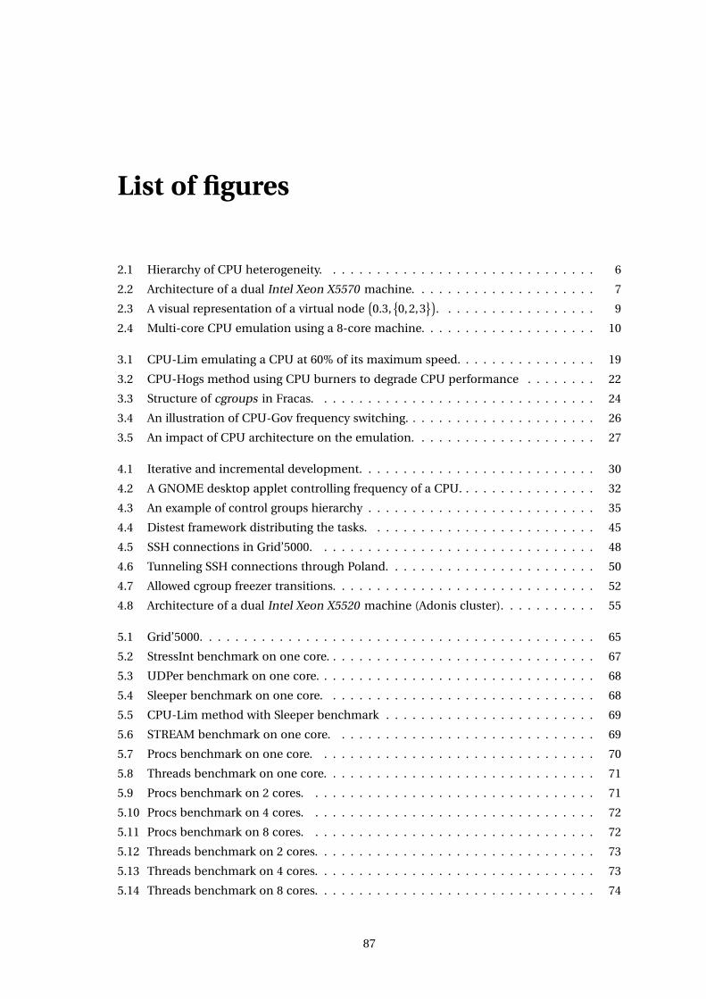
List of figures
2.1 Hierarchy of CPU heterogeneity. . . . . . . . . . . . . . . . . . . . . . . . . . . . . . . 6
2.2 Architecture of a dual Intel Xeon X5570 machine. . . . . . . . . . . . . . . . . . . . . 7
2.3 A visual representation of a virtual node(0.3,
{0,2,3
}). . . . . . . . . . . . . . . . . . 9
2.4 Multi-core CPU emulation using a 8-core machine. . . . . . . . . . . . . . . . . . . . 10
3.1 CPU-Lim emulating a CPU at 60% of its maximum speed. . . . . . . . . . . . . . . . 19
3.2 CPU-Hogs method using CPU burners to degrade CPU performance . . . . . . . . 22
3.3 Structure of cgroups in Fracas. . . . . . . . . . . . . . . . . . . . . . . . . . . . . . . . 24
3.4 An illustration of CPU-Gov frequency switching. . . . . . . . . . . . . . . . . . . . . . 26
3.5 An impact of CPU architecture on the emulation. . . . . . . . . . . . . . . . . . . . . 27
4.1 Iterative and incremental development. . . . . . . . . . . . . . . . . . . . . . . . . . . 30
4.2 A GNOME desktop applet controlling frequency of a CPU. . . . . . . . . . . . . . . . 32
4.3 An example of control groups hierarchy . . . . . . . . . . . . . . . . . . . . . . . . . . 35
4.4 Distest framework distributing the tasks. . . . . . . . . . . . . . . . . . . . . . . . . . 45
4.5 SSH connections in Grid’5000. . . . . . . . . . . . . . . . . . . . . . . . . . . . . . . . 48
4.6 Tunneling SSH connections through Poland. . . . . . . . . . . . . . . . . . . . . . . . 50
4.7 Allowed cgroup freezer transitions. . . . . . . . . . . . . . . . . . . . . . . . . . . . . . 52
4.8 Architecture of a dual Intel Xeon X5520 machine (Adonis cluster). . . . . . . . . . . 55
5.1 Grid’5000. . . . . . . . . . . . . . . . . . . . . . . . . . . . . . . . . . . . . . . . . . . . . 65
5.2 StressInt benchmark on one core. . . . . . . . . . . . . . . . . . . . . . . . . . . . . . . 67
5.3 UDPer benchmark on one core. . . . . . . . . . . . . . . . . . . . . . . . . . . . . . . . 68
5.4 Sleeper benchmark on one core. . . . . . . . . . . . . . . . . . . . . . . . . . . . . . . 68
5.5 CPU-Lim method with Sleeper benchmark . . . . . . . . . . . . . . . . . . . . . . . . 69
5.6 STREAM benchmark on one core. . . . . . . . . . . . . . . . . . . . . . . . . . . . . . 69
5.7 Procs benchmark on one core. . . . . . . . . . . . . . . . . . . . . . . . . . . . . . . . 70
5.8 Threads benchmark on one core. . . . . . . . . . . . . . . . . . . . . . . . . . . . . . . 71
5.9 Procs benchmark on 2 cores. . . . . . . . . . . . . . . . . . . . . . . . . . . . . . . . . 71
5.10 Procs benchmark on 4 cores. . . . . . . . . . . . . . . . . . . . . . . . . . . . . . . . . 72
5.11 Procs benchmark on 8 cores. . . . . . . . . . . . . . . . . . . . . . . . . . . . . . . . . 72
5.12 Threads benchmark on 2 cores. . . . . . . . . . . . . . . . . . . . . . . . . . . . . . . . 73
5.13 Threads benchmark on 4 cores. . . . . . . . . . . . . . . . . . . . . . . . . . . . . . . . 73
5.14 Threads benchmark on 8 cores. . . . . . . . . . . . . . . . . . . . . . . . . . . . . . . . 74
87
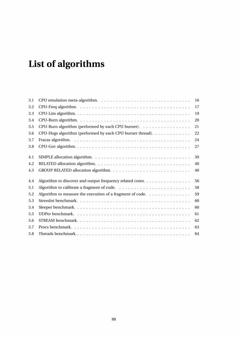
List of algorithms
3.1 CPU emulation meta-algorithm. . . . . . . . . . . . . . . . . . . . . . . . . . . . . . . 16
3.2 CPU-Freq algorithm. . . . . . . . . . . . . . . . . . . . . . . . . . . . . . . . . . . . . . 17
3.3 CPU-Lim algorithm. . . . . . . . . . . . . . . . . . . . . . . . . . . . . . . . . . . . . . . 19
3.4 CPU-Burn algorithm. . . . . . . . . . . . . . . . . . . . . . . . . . . . . . . . . . . . . . 20
3.5 CPU-Burn algorithm (performed by each CPU burner). . . . . . . . . . . . . . . . . 21
3.6 CPU-Hogs algorithm (performed by each CPU burner thread). . . . . . . . . . . . . 22
3.7 Fracas algorithm. . . . . . . . . . . . . . . . . . . . . . . . . . . . . . . . . . . . . . . . 24
3.8 CPU-Gov algorithm. . . . . . . . . . . . . . . . . . . . . . . . . . . . . . . . . . . . . . . 27
4.1 SIMPLE allocation algorithm. . . . . . . . . . . . . . . . . . . . . . . . . . . . . . . . . 39
4.2 RELATED allocation algorithm. . . . . . . . . . . . . . . . . . . . . . . . . . . . . . . . 40
4.3 GROUP RELATED allocation algorithm. . . . . . . . . . . . . . . . . . . . . . . . . . . 40
4.4 Algorithm to discover and output frequency related cores. . . . . . . . . . . . . . . . 56
5.1 Algorithm to calibrate a fragment of code. . . . . . . . . . . . . . . . . . . . . . . . . 58
5.2 Algorithm to measure the execution of a fragment of code. . . . . . . . . . . . . . . 59
5.3 StressInt benchmark. . . . . . . . . . . . . . . . . . . . . . . . . . . . . . . . . . . . . . 60
5.4 Sleeper benchmark. . . . . . . . . . . . . . . . . . . . . . . . . . . . . . . . . . . . . . . 60
5.5 UDPer benchmark. . . . . . . . . . . . . . . . . . . . . . . . . . . . . . . . . . . . . . . 61
5.6 STREAM benchmark. . . . . . . . . . . . . . . . . . . . . . . . . . . . . . . . . . . . . . 62
5.7 Procs benchmark. . . . . . . . . . . . . . . . . . . . . . . . . . . . . . . . . . . . . . . . 63
5.8 Threads benchmark. . . . . . . . . . . . . . . . . . . . . . . . . . . . . . . . . . . . . . . 64
88
Bibliography
[AJ97] Andrzej Jaszkiewicz. Inzynieria oprogramowania. Helion, Gliwice, Poland, 1997.
[BCOM+10] François Broquedis, Jérôme Clet Ortega, Stéphanie Moreaud, Nathalie Furmento, Brice
Goglin, Guillaume Mercier, Samuel Thibault, and Raymond Namyst. hwloc: a Generic
Framework for Managing Hardware Affinities in HPC Applications. In The 18th
Euromicro International Conference on Parallel, Distributed and Network-Based
Computing (PDP 2010), 2010.
[BNG10a] Tomasz Buchert, Lucas Nussbaum, and Jens Gustedt. Accurate emulation of CPU
performance. In 8th International Workshop on Algorithms, Models and Tools for
Parallel Computing on Heterogeneous Platforms - HeteroPar’2010, Ischia Italie, 08 2010.
[BNG10b] Tomasz Buchert, Lucas Nussbaum, and Jens Gustedt. Methods for Emulation of
Multi-Core CPU Performance. Research Report RR-7450, INRIA, 11 2010.
[BOC] Bochs documentation. http://bochs.sourceforge.net/.
[CCD+05] Franck Cappello, Eddy Caron, Michel Dayde, Frederic Desprez, Emmanuel Jeannot, Yvon
Jegou, Stephane Lanteri, Julien Leduc, Nouredine Melab, Guillaume Mornet, Raymond
Namyst, Pascale Primet, and Olivier Richard. Grid’5000: a large scale, reconfigurable,
controlable and monitorable Grid platform. In Grid’2005 Workshop, Seattle, USA, 2005.
[CCR+03] Brent Chun, David Culler, Timothy Roscoe, Andy Bavier, Larry Peterson, Mike
Wawrzoniak, and Mic Bowman. Planetlab: an overlay testbed for broad-coverage
services. SIGCOMM Comput. Commun. Rev., 33(3):3–12, 2003.
[CDGJ10] Louis-Claude Canon, Olivier Dubuisson, Jens Gustedt, and Emmanuel Jeannot.
Defining and Controlling the Heterogeneity of a Cluster: the Wrekavoc Tool. Journal of
Systems and Software, 83:786–802, 2010.
[CEL] Cell (microprocessor) - Wikipedia, the free encyclopedia.
http://en.wikipedia.org/wiki/Cell_(microprocessor).
[CFS] Kernel Documentation of CFS Scheduler. http://lxr.linux.no/linux+v2.6.34/Documentation/scheduler/sched-design-CFS.txt.
[DG04] Jeffrey Dean and Sanjay Ghemawat. Mapreduce: Simplified data processing on large
clusters. In OSDI (Operating System Design and Implementation), pages 137–150, 2004.
[FRE] Kernel Documentation of Freezer Subsystem. http://lxr.linux.no/#linux+v2.6.36/Documentation/cgroups/freezer-subsystem.txt.
[G5K] The Grid’5000 experimental testbed. https://www.grid5000.fr.
89
90 Bibliography
[GJQ09] Jens Gustedt, Emmanuel Jeannot, and Martin Quinson. Experimental Validation in
Large-Scale Systems: a Survey of Methodologies. Parallel Processing Letters, 19:399–418,
2009.
[GVV08] Diwaker Gupta, Kashi V. Vishwanath, and Amin Vahdat. Diecast: testing distributed
systems with an accurate scale model. In Proceedings of the 5th USENIX Symposium on
Networked Systems Design and Implementation, 2008.
[HPC] HPC Challenge Benchmark. http://icl.cs.utk.edu/hpcc/.
[Jon] M. Tim Jones. Inside the Linux 2.6 Completely Fair Scheduler: Providing fair access to
CPUs since 2.6.23. http://www.ibm.com/developerworks/linux/library/l-completely-fair-scheduler/.
[KAF+10] Thorsten Kleinjung, Kazumaro Aoki, Jens Franke, Arjen Lenstra, Emmanuel Thomé,
Joppe Bos, Pierrick Gaudry, Alexander Kruppa, Peter Montgomery, Dag Arne Osvik,
Herman te Riele, Andrey Timofeev, and Paul Zimmermann. Factorization of a 768-bit rsa
modulus. Cryptology ePrint Archive, Report 2010/006, 2010.
http://eprint.iacr.org/.
[McC07] John D. McCalpin. Stream: Sustainable memory bandwidth in high performance
computers. Technical report, University of Virginia, Charlottesville, Virginia, 1991-2007.
A continually updated technical report. http://www.cs.virginia.edu/stream/.
[MPM] mpmath - python library for arbitrary-precision floating-point arithmetic.
http://code.google.com/p/mpmath/.
[OAR] Oar resource manager. http://oar.imag.fr/.
[PH10] Swann Perarnau and Guillaume Huard. Krash: reproducible CPU load generation on
many cores machines. In IPDPS ’10: Proceedings of the 2010 IEEE International
Symposium on Parallel & Distributed Processing, 2010.
[RW73] Horst W. J. Rittel and Melvin M. Webber. Dilemmas in a general theory of planning.
Policy Sciences, 4(2):155–169, June 1973.
[SLJ+00] H. J. Song, X. Liu, D. Jakobsen, R. Bhagwan, X. Zhang, K. Taura, and A. Chien. The
Microgrid: a Scientific Tool for Modeling Computational Grids. In Proceedings of IEEE
Supercomputing, 2000.
[The04] The IEEE and The Open Group. The Open Group Base Specifications Issue 6 – IEEE Std
1003.1, 2004 Edition. IEEE, New York, NY, USA, 2004.
[TOP] TOP500 Supercomputing Sites. http://www.top500.org/.
[VYW+02] Amin Vahdat, Ken Yocum, Kevin Walsh, Priya Mahadevan, Dejan Kostic, Jeff Chase, and
David Becker. Scalability and accuracy in a large-scale network emulator. SIGOPS Oper.
Syst. Rev., 36(SI):271–284, 2002.
[WLS+02] Brian White, Jay Lepreau, Leigh Stoller, Robert Ricci, Shashi Guruprasad, Mac Newbold,
Mike Hibler, Chad Barb, and Abhijeet Joglekar. An integrated experimental environment
for distributed systems and networks. In OSDI’02, Boston, MA, 2002.
[ZIP+10] Boxun Zhang, Alexandru Iosup, Johan A. Pouwelse, Dick H. J. Epema, and Henk J. Sips.
Sampling bias in bittorrent measurements. In Euro-Par (1), pages 484–496, 2010.

© 2010 Tomasz Buchert
Poznan University of TechnologyFaculty of Computing Science and ManagementInstitute of Computing Science
Typeset using LATEX.
BibTEX:
@mastersthesis{ key,author = "Tomasz Buchert",title = "{Methods for Emulation of Multi-Core CPU Performance}",school = "Poznań University of Technology",address = "Pozna{\’n}, Poland",year = "2010",
}