102 3&( 545 6

�� !�#"$%�'&(�*)+��!�,��-�'&(&*� �!).� �$&*�, ��/��102��3&(� �545��6��(� �!��!�.�3&*�879�:&��3��;�&*�*"$;��<�=�>�?"�� @�3&�;.A

BCED F.F�DHG#I+J�K(L B:M N/O J�P!J:Q.K(Q.R�Q.S.L B�M R8T>Q B L�J�PVUXW3G O T�Y�Z9[\J�K(I+L�](]!L%Q N P(Q_^�]!J�`�S.^�K!Ja]�b�P Mcd R�J:]:b M Nfe d K(L%J�ghJ�i B J:K!j�P(],gkK!Q'IlP!m�Ln]+opQ'K!q-L N ] B L�J N P!L%` BrM N�e J e ^ B:M P(L%Q N�M R�opQ'K!qs]tL�]m�J:K!J d U�S.K M N P!J e j�K!Qu>L e J e P(m M P2P!m�Jt]!Q.^�K B J�L�] M.B q N QovR�J e S'J e ZwG N Ur^�]xJtQ g�I M P!J:K!L M RL N P!m�Ln]�opQ'K!q,P!m M PpLn] e J�P(J�K(IHL N J e P!Q d J1yg M L%Kp^�]xJayz^ Nfe J�KvT>J B P!L�Q N/{ F�|1Q'K}P(m M Pv] M P!Ln] c`�Ja]~P(m�J B Q N�e L%P!L�Q N ]�]xj$J B L<`fJ e L N T>J B P!L�Q N�{ F.�tQ g8P(m�J��zZ�T�Zf�pQ.j>U>K(L%S'm'P�� M o�W { |t�2T��2bM ]2K(J�u>L�]!J e d U/[\Z �}Z�� c��'� � Y e Q�Ja] N Q P�K!Ja�'^�L%K(JzP(m�J+TsQ B L%J�PVU�� ]2jfJ:K!I+Ln]!]!L�Q N Z��vJ�j�^ d R�L cB�M P!L�Q N b�]!Us]VP(J�I M P(L B K(J�j�K!Q e ^ B P!L�Q N bsj$Q']xP!L N S�L N J�R�J B P!K(Q N L B gkQ.K(I�Q N ]!J�K(u.J�K*]:b�Q'K#Q P(m�J�K^�]!J:]�Q.g2P(m�Ln]�I M P!J:K!L M R�bwJ�i B J:jsP M ]+J�isJ�I+jsP!J e d U�P!m�J M d Qu.J�]xP M P(J�I+J N P*]�b�K!Ja��^�L%K(J:]ovK(L<P!P!J N j$J�K(IHLn](]xL�Q N Q.KvR�L B J N ]!J1gkK!Q'I�P!m�JzG O T�Z�G e�e L%P!L�Q N�M R e J�P M L�R�] M K!J1j�K(Qu�L e J e L NP!m�J_G O T��pQ'j�U>K(L%S'm�P�[\Q'R%L B L�J:]:b M u M L�R M d R�JHgkK!Q'I�P!m�J�G O T M Pt� { | c D.D'| c D ��D � Q.K M I c]!j�^ d ]�� M I+J�P*]xQ B Z Q'K!SfZ

[\J�K(I+L�](]!L%Q N P!Qtj�R M'B J MtB Q'j>UHQ.g8P!m�L�]�o�Q.K(qHQ N P!m�L�]v]!J�K(u.J:K~m M ] d J�J N j�K(Qu>L e J e d U+P!m�JG O T�Z��wm�J�G O T e Q>J:] N Q PwS.^ M K M.N P(J�JhP!m M P�P(m�J B Q'j�U�j�K!Qu>L e J e m�J�K(J2Ln] M NrM.B:B ^�K M P(JB Q'j>U�Q g�P!m�J�j�^ d R%Ln]!m�J e o�Q.K(q$Z

FEBRUARY 2002 585L I L L Y A N D R H I N E S

q 2002 American Meteorological Society

Coherent Eddies in the Labrador Sea Observed from a Mooring

JONATHAN M. LILLY AND PETER B. RHINES

School of Oceanography, University of Washington, Seattle, Washington

(Manuscript received 17 February 2000, in final form 23 January 2001)

ABSTRACT

During June–November 1994, a mooring in the central Labrador Sea near the former Ocean Weather StationBravo recorded a half-dozen anomalous events that prove to be two different types of coherent eddies. Com-parisons with simple analytical models are used to classify these events as coherent eddies on the basis of theirvelocity signatures. The first clear examples of long-lived convectively generated eddies are reported. Thesefour small (radius ;5–15 km) eddies are exclusively anticyclonic, with cold, fresh middepth potential temperature(u) and salinity (S) cores surrounded by azimuthal currents of ;15 cm s21. Their u/S properties identify themunambiguously as the products of wintertime deep convection in the interior Labrador Sea. Compared witheddies in other regions, these anticyclones are unusual for their strong surface expressions and composite u/Scores. Two warm cyclones are also seen; these are larger (radius ;15 km) than the anticyclones and about asenergetic (currents ;15 cm s21). Their u/S and potential vorticity properties suggest that they are created bystretching a column of water from the Irminger Current, which surrounds the Labrador Sea on three sides.

1. Introduction

The coherent eddy field plays an important role inconvective regions such as the Labrador Sea. Baroclinic,property-carrying eddies are expected to mediate thedispersal of convected water from a well-convectedpatch into the ambient sea (Legg and Marshall 1993;Send and Marshall 1995), as well the restratification ofthe water column following deep convection (Jones andMarshall 1997). Convectively generated deformation-scale eddies have been observed in the Labrador Seausing floats and hydrography by Gascard and Clarke(1983). However, direct measurements of the effects ofsuch eddies, in the Labrador Sea or elsewhere, remainelusive (Marshall and Schott 1999, 107–108). Coherenteddies may be important to deep convection in anotherway: cyclonic eddies can destabilize the upper watercolumn, ‘‘preconditioning’’ it for deep convection (Legget al. 1998; Straneo and Kawase 1999).

The Labrador Sea, the site of deep convection reach-ing a depth of over 2 km during some winters, is ofparticular importance for its influence on the u/S andpotential vorticity structure of the North Atlantic (Talleyand McCartney 1982) and as a potentially sensitive lo-cation for the thermohaline circulation (Hakkinen 1999).Convection there has long been known to account forboth annual and interannual variations in the water-mass

Corresponding author address: Jonathan M. Lilly, School ofOceanography, University of Washington, Box 347940, Seattle, WA98195.E-mail: [email protected]

properties (Lazier 1973, 1980) and to involve organi-zations across a range of scales, from submesoscale tobasin-scale (Clarke and Gascard 1983; Gascard andClarke 1983).

For these reasons a long-term mooring, located at56.758N, 52.58W (Fig. 1) near the site of the formerOcean Weather Station (OWS) Bravo, was establishedto monitor interannual variability in the central LabradorSea. The present work is the second involving the Bravomooring; the first (Lilly et al. 1999, hereafter LS99)described one annual ‘‘cycle’’ of u/S properties and cur-rents for the year June 1994–June 1995. Here we focuson the nonconvecting period June–November 1994 todevelop methods for investigating the structure of co-herent eddies from a mooring.

2. Data and methods

The data used for this paper were described in detailin LS99, but we will summarize here. The primary data(see Table 1) are from six SeaBird SBE 16 SEACATsmeasuring temperature and conductivity, and six Aan-deraa RCM-8 instruments measuring current speed anddirection as well as temperature, all sampling at hourlyintervals. Pressure was measured at two instruments,allowing us construct a pressure record at all depthsthrough the use of a mooring model. All temperaturedata were recast into potential temperature, using a fixedsalinity profile for those instruments that lacked salinity.Temperature and salinity data were calibrated againstendpoint CTD casts.

The inertial wave/semidiurnal tidal band has an am-

586 VOLUME 32J O U R N A L O F P H Y S I C A L O C E A N O G R A P H Y

FIG. 1. Map of the Labrador Sea showing the location of the Bravomooring (triangle) at 56.758N, 52.58W. The station locations of the1994 World Ocean Circulation Experiment (WOCE) AR7W hydro-graphic line are indicated by filled circles. The contour interval forthe bathymetry (gray) is 500 m, the innermost contour intersected bythe AR7W line being the 3500-m isobath.

TABLE 1. Bravo mooring instrumentation 1994–95. Measurementsare ‘‘t’’ for temperature, ‘‘c’’ for conductivity, ‘‘p’’ for pressure,‘‘spd’’ for current speed, and ‘‘dir’’ for current direction.

Depth(m) Instrument Measurement

110260510760

1010126015101760201025103476

Aanderaa RCM-8SeaBird 16 SEACATSeaBird 16 SEACATAanderaa RCM-8SeaBird 16 SEACATAanderaa RCM-8SeaBird 16 SEACATAanderaa RCM-8SeaBird 16 SEACATSeaBird 16 SEACATAanderaa RCM-8

spd, dir, t, pt, ct, cspd, dir, tt, c, pspd, dir, tt, cspd, dir, tt, ct, cspd, dir, t

FIG. 2. A CTD section along the AR7W line between Labrador(left) and Greenland (right). Salinity is shown as shading, with a verynarrow range emphasizing the freshest water in the interior. Contoursof potential density s1500 are also shown. Thin vertical lines denotethe locations of CTD stations, and the location of the Bravo mooringis shown by a dashed white line.

plitude of typically 5 cm s21 (10 cm s21 peak-to-peak)and so is a signal roughly half the magnitude of thatdue to the eddies. All time series are therefore filteredwith a 24-h Hanning filter; this length filter was foundto be the best compromise between removing tidal noiseand keeping high-frequency fluctuations due to eddies.

The density signal of the eddies is small and verysensitive to choice of reference level. At each instrumentwe define a quantity

s 5 r(s, t, p, p)L (1)

where is the average instrument pressure, which weprefer to as the locally referenced potential density. An-other useful quantity is the isopycnal displacement DZs,which we find by interpolating sL within a vertical pro-file derived from CTD data. This is useful for compar-isons across different depths, but has a high noise levelin the central water column owing to the weak strati-fication.

3. Eddylike events in the mooring data

The flow in the interior Labrador Sea (see LS99) isnearly barotropic and highly variable. For the June–November 1994 period that this paper focuses on, themagnitude of the mean vertically averaged current is4.1 cm s21 to the southwest, and its standard deviation

is 11.4 cm s21. Over 90% of the energy can be accountedfor by the barotropic mode. Departures from barotropicflow are found not only in the upper water column butalso and primarily in the lowest kilometer. This shearstructure reflects the stratification (Figs. 2, 3), whichconsists of the weakly stratified Labrador Sea Water(LSW) between about 500 and 2000 m depth sand-wiched between a ;500 m thick stratified layer at thesurface and an ;1 km stratified layer at the bottom.The linear, flat-bottom vertical modes computed fromthe CTD data show that the first baroclinic mode has


FIG. 3. The vertical structure of the interior Labrador Sea, from CTD casts during Jun 1994. (a) Potential temperature u (black) and salinity(gray). (b) Potential density s1500 (black) and buoyancy frequency from vertically smoothed data (gray). The average of all the individualbuoyancy frequency profiles is also shown. (c) The horizontal structure function from a modal decomposition (using the rigid-lid approxi-mation) of section-averaged, 50-m decimated N 2 profiles.

the upper 2 km and lower 1 km out of phase, with acorresponding deformation radius of 7 km. This modedominates the baroclinic signal in the mooring data.

The currents measured during June–November 1994in the central water column contain a number of suddenrotational events, seen in a stick-vector plot (Fig. 4a)and especially in the time series of u and y (Fig. 4b).These transitions in the velocity field tend to be asso-ciated with extrema of the isopycnal displacement ob-served at 2500 m (and other depths), as well as withupper-level temperature anomalies (Figs. 4c,d); similardepressions of the deep stratification associated with u/S anomalies are occasionally observed in the CTD data(Fig. 2). Six events (A–F) are marked, each of whichhas a temperature anomaly (anywhere in the water col-umn) greater than 0.058C, an isopycnal displacementmagnitude greater than 100 m, and a velocity anomalygreater than 10 cm s21; no other events during this timeperiod meet all three criteria. We will argue that thesesix events are advected eddies.

Vertical–temporal ‘‘slices’’ through each of theseevents (Fig. 5) reveal eddylike structures, with a mid-depth u/S core surrounded by a ring of strong currents.

Here the velocity has been rotated into components (up,y n) parallel to and normal to the estimated advectingflow, with the normal component y n shown. As dis-cussed in the following section, the dominant signal ofan advected eddy is expected to be in the normal com-ponent, with y n initially positive (negative) for a cyclone(anticyclone). Events C and D thus appear to be cycloniceddies, while the others are anticyclones.

Figure 6 shows the hodograph (the curve traced outby the tip of the velocity vector with time) and its in-tegral, the progressive vector diagram, for the velocitytime series shown in Figs. 4a and 4b. The shading isthe potential temperature at 1010 m, detrended to re-move a slow warming. The six events A–F are all as-sociated with a 10 cm s21 or larger turning of the ve-locity vector, the edges of which coincide with the edgesof a temperature anomaly. Within the temperature anom-aly the hodograph tends to be relatively straight, and oneither side are found regions having the opposite rota-tion sense from the central region. The progressive vec-tor diagram has bends at the locations of these events,with bends to the right (left) associated with the apparentcyclones (anticyclones).


FIG. 4. Velocity transitions during the 6-month period Jun–Nov1994. (a) Stick vectors at 1260 m with approximately one stick perday shown. The u and y time series shown here as well as all othertime series data in this paper have been smoothed with a 24-h Hanningfilter. Vertical lines mark the locations of sudden rotations of thevelocity that are shown to be due to the advection of small-scaleeddies. (b) Time series of u (solid) and y (dashed) at 1260 m. (c)Isopycnal displacement DZs at 2500 m. (d) Potential temperature uat 1010 m.

The vertical slices as well as the temporal structureof the currents support the diagnosis of these six eventsas advected coherent eddies. This argument is strength-ened by comparison with analytical models in the fol-lowing section. Some readers may wish to turn imme-diately to the physical description of events A–F givenin section 5.

4. Kinematic models of eddy advection

Inferring the two-dimensional (x, y) nature of an eventbased on its (u, y) signature at a single point is inherentlycomplicated and warrants a careful examination of the

expected currents due to an advected eddy and otherbasic structures.

a. An isolated eddy

Let an eddy be advected by a spatially uniform buttime-varying flow � (t) 1 i � (t) so that the eddy’s tra-jectory can be represented by a curve on the complexplane

if (t)h(t) [ r9(t)e [ x9(t) 1 iy9(t) 5 � 1 i � dt.EThe currents observed by a mooring at the origin are

ifj(t) [ � 1 i � 2 ie y (r9)

and the currents due to the eddy only are

ifj9(t) [ j 2 ( � 1 i � ) 5 2ie y (r9), (2)

where (r) describes the radial velocity profile of thisy(azimuthally symmetric) eddy and is positive for cy-clonic currents. Equation (2) states that an eddy’s tra-jectory, modified by the azimuthal velocity profile, trac-es out the currents observed at a mooring. The mag-nitude of the eddy currents is simply given by the dis-tance from the mooring to the eddy center r9(t) throughthe azimuthal velocity profile as

| j9(t) | 5 | y (r9(t)) | .

The orientation of the eddy currents is given by rotatingh, the line from the mooring location to the eddy center,90 degrees counterclockwise through the factor 2ieif(t).An obvious but surprisingly useful consequence of (2)is that the eddy currents are always perpendicular to h.

A very simple model eddy consists of solid-body ro-tation within a core (r , R) and 1/r decay elsewhere,

21VrR , r , Ry (r) 5 (3)

215VRr , r . R,

and is known as the Rankine vortex. Here V is the max-imum azimuthal velocity (positive for a cyclone). If theflow is in quasigeostrophic balance, the Rankine vortexis the solution to a uniform potential vorticity (PV)anomaly within radius R of magnitude q 5 2V/R.

The currents observed by a north–south array ofmoorings as a Rankine vortex is advected past by aconstant eastward flow U (Fig. 7) are even in the parallel(eastward) direction and odd in the normal (northward)direction. The resulting hodographs (Fig. 7b) arestraight lines when the mooring is inside the eddy coreand circles when the mooring is outside the core. Theends of the hodograph return to the value of the meanflow as the distance to the eddy center becomes large.For ‘‘slices’’ that intersect the eddy core, the combi-nation of a straight line with a segment of a circle resultsin a ‘‘D’’ shape with the flat part of the ‘‘D’’ perpen-dicular to the advecting flow. The nearer the slice to the


FIG. 5. Potential temperature u and normal velocity y n cross sections through eddies A–F. Identical time windows and contours are usedfor each event. Black lines are contours of potential temperature, measured at 11 instruments. The contour interval is 0.018C with labelingevery 0.058C. Gray lines are contours of normal velocity y n (measured at six instruments) every 2 cm s21 with labeling every 4 cm s21;negative contours are dashed. Normal velocity is negative for early times for advected anticyclones (A, B, E, F) and positive for advectedcyclones (C, D).

center of the eddy, the more the hodograph collapsesonto a straight line.

The reasons for the straight lines and circles can beseen by considering (2) for the specific case of a Rankinevortex, which becomes

212iR Vh, zh z , Rj9(t) 5 (4)

2152ih* VR, zh z . R.

In the interior of the Rankine vortex, the eddy velocityvector j9 is simply the displacement vector h rotated 90degrees clockwise and rescaled by a constant. Solid-body rotation therefore maps a straight line on the (x, y)plane onto a perpendicular straight line on the (u, y)plane. In particular, for an eddy advected by a constanteastward flow U the eddy location h is

h 5 x9 1 iy9 5 U(t 2 t ) 1 id,o

so that the x location of the eddy center is linear withtime and the y location (denoted d) is constant. It followsfrom (4) that

21 21j9 5 u9 1 iy9 5 R Vd 2 iR VU(t 2 t )o

so that u9 is constant and y9 is linear with time, as canbe seen in Figs. 7c,d. Outside of the eddy’s core, ;yr21, and basic complex analysis applied to (4) showsthat a straight line h 5 U(t 2 to) 1 id maps onto acircle of diameter | d21VR | touching the point U 1 0i.

b. Other features

The D-shaped structures on the hodograph plane re-flect the two-dimensional (x, y) structure of the eddies.By contrast the advection of a feature that is invariantin one dimension, such as a front or a filament, willresult in a straight line on the (u, y) plane, as with thecase of an eddy sliced through its exact center. Since afront can have any orientation with respect to the ad-vecting flow, this straight line on the (u, y) plane neednot be perpendicular to � 1 i � . Hodographs due tocurved filaments are complicated (because a stronglycurved filament will tend to be intersected twice) and


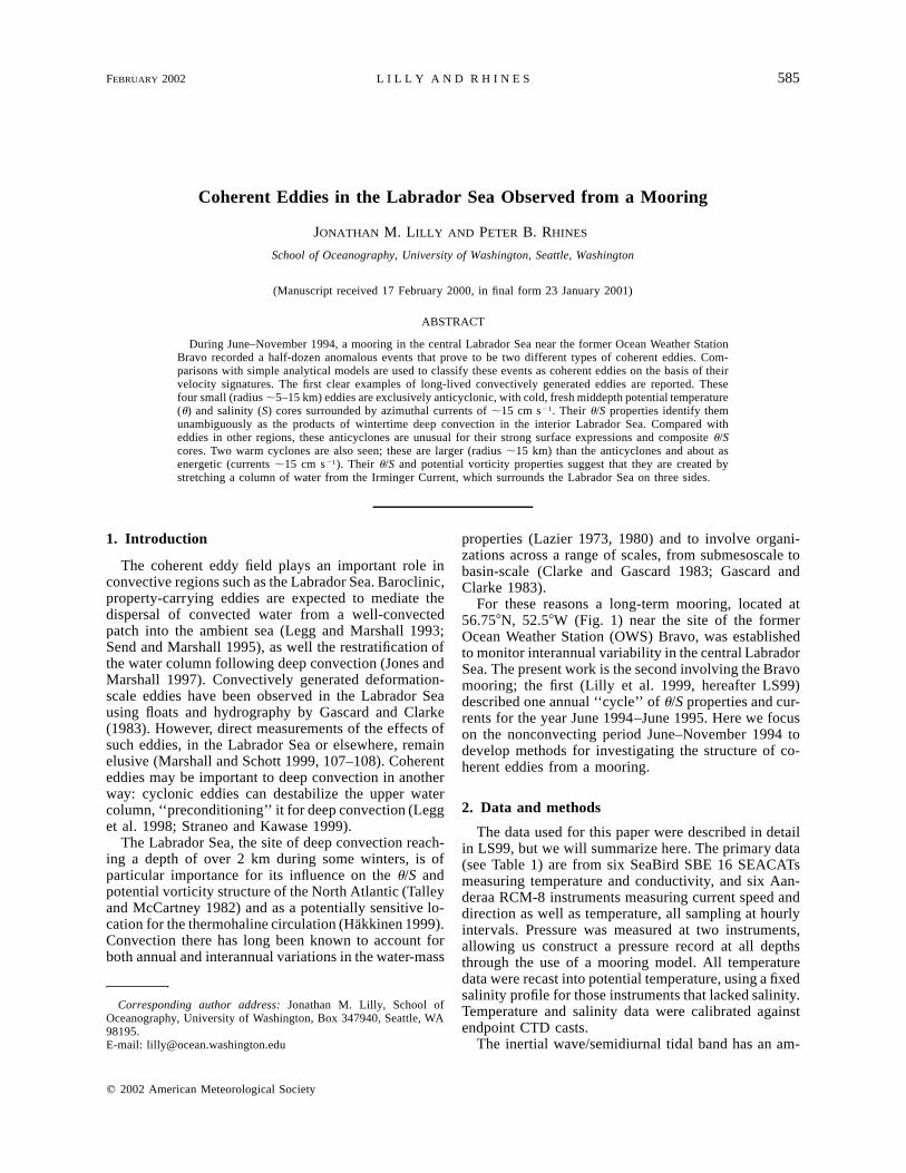
FIG. 6. (a) Hodograph of the currents observed at 1260 m for the time period Jun–Dec. Color denotes potential temperature at 1010 m,detrended over this time period to remove a slow warming. Six events that resemble advected eddies have been marked. The estimatedcenters of these events have been marked with circles (cold anticyclones) and triangles (warm cyclones). (b) Progressive vector diagram for1260 m (upper curve) as well as for 3476 m (lower curve). Color is the same as for (a).

bear little resemblance to those in Fig. 6; neither do thehodographs of a front or filament advected by an os-cillatory flow. In general it seems difficult for fronts orfilaments to result in hodographs similar to those ofadvected eddies sliced off-center.

Different velocity profiles (r) will, obviously, resultyin different hodographs, but the differences are not dra-matic. For an eddy that has a radial velocity profileproportional to (r/R)m for m ± 1 the solid-body line willbecome deformed, and will bow inward for m . 1 oroutward for m , 1. Using a Gaussian streamfunctionprofile, which corresponds to a more diffuse core thanthe observations, results in more gently curving hodo-graphs and an outward bowing of the solid-body line.Similarly, a two-layer model with a PV anomaly in theupper layer only (using realistic parameters for the Lab-rador Sea) results in a more rapid (,r21) decay rateoutside of the core, but for deformation-scale eddies thehodographs are virtually unchanged.

The hodographs for a self-advecting dipole (notshown) are similar to those of an advected monopolareddy only when the dipole is sliced near the location ofone of its vorticity cores and when the background flowis negligible. When a dipole is sliced in between the twocores, the result is an impulsive feature: the currents sud-denly accelerate and then decelerate, with the amount ofrotation decreasing as the location of the slice approachesthe centerline of the dipole. In general, a dipole willpropagate at an angle to the advecting flow due to its

self-advection, leading to ‘‘tilted’’ hodographs that areperpendicular to the direction of net propagation ratherthan to the advecting flow. Event C has a tilted hodographthat may be due to a self-advecting component. Sincethe other eddies observed at the mooring appear to beassociated with an O(10 cm s21) advecting flow but theirsolid-body lines are not tilted, these features are not con-sistent with strongly self-advecting dipoles.

c. An eddy field

The data resemble the model in that roughly straight-line regions of the hodographs perpendicular to the ap-parent background flow (with the exception of event C)are associated with temperature anomalies. The mostnoticeable difference between the data and the constantadvecting flow model is that in the data the hodographsoften do not ‘‘close’’ completely.

In the central Labrador Sea the assumption of a con-stant advecting flow is clearly unrealistic. An alternatemodel is a field of Rankine vortices. As a first approx-imation an eddy is assumed to be advected by the netvelocity felt at its exact center, as in a point vortexmodel. Eddies of similar size and strength, plus a smallrandom component, are initially placed on a grid, againplus a random offset. An example of a hodograph andprogressive vector diagram resulting from this model isshown in Figs. 8a and 8b (see caption for model details).Hodographs no longer decay to a fixed point, but can


FIG. 7. An advected cyclonic model eddy ‘‘sliced’’ by an array of moorings. (a) The eddy currents in plan view in the reference framemoving with the eddy. The maximum speed, at the eddy rim (gray circle), is 10 cm s21. Horizontal lines are the paths the moorings takethrough the eddy, with black and gray lines denoting trajectories passing on opposite sides of the eddy core. (b, c, d) The currents observedat each of the eight moorings as the eddy is advected past them. (b) Hodographs of the observed currents, with the advecting flow (2.5 cms21 to the east) shown by an arrow. (c) Eastward, or parallel, component of the velocity. The eddy rim for a slice through the exact centeris marked with vertical lines in this and the following plot. (d) Northward, or perpendicular, velocity component.

in general be ‘‘open’’ or ‘‘closed.’’ The appearance ofeddies in the eddy-field model can be qualitatively verysimilar to events A–F. Hodographs can therefore be eas-ily deformed through the presence of other eddies orperhaps by other low-frequency flow components intofeatures like those observed at the mooring.

5. Structure of observed eddies

In the previous sections we argued that six majorevents of June–November 1994 were advected coherenteddies. We now describe them in greater detail.

Estimating the structure of a coherent eddy from a


FIG. 8. (a) Hodograph from a realization of an idealized eddy-field model. In this model, at time to 64 Rankine vortices are located on aregular grid plus a small random perturbation. The eddies have | 5 1 G | km radius, where G is a unit variance Gaussian random variable,and maximum azimuthal currents of random sign and magnitude 10 1 2.5G cm s21. The initial spacing is 50 km in both x and y directions,and each eddy’s center is perturbed by 12.5G km in both directions. The eddy field is integrated in time with a time step of 1 h for 2048hours in the forward and reverse directions from t 5 to, with each eddy being advected by the total velocity at its exact center. The hodographis from a mooring at the center of the eddy grid. Black dots denote times when the mooring is inside an eddy’s core; gray dots denote othertimes. (b) The progressive vector diagram for the time series whose hodograph is shown in (a).

TABLE 2. Estimated eddy parameters: DT: the temporal half-duration of an eddy, Ua (Xa): the estimated mean flow speed (eddy apparentradius) using the ‘‘angle’’ method, Uf (Xf): the estimated mean flow speed (eddy apparent radius) using the ‘‘filtering’’ method, Vn (VU): theestimated maximum eddy currents using the ‘‘normal’’ (‘‘U subtraction’’) method, � : the range of estimated Rossby numbers using thevarious values for V and X, Dz: the vertical difference between levels of maximum isopycnal displacement, and the Ds: the eddy’s maximumdensity anomaly. See text for details.

A B C D E F

DT (h)Ua (cm s21)Uf (cm s21)Xa (km)Xf (km)Vn (cm s21)VU (cm s21)

�Dz (km)Ds (1023 g kg21)

536.3

12.511.923.8

217.2217.80.12–0.24

1.25 6 0.2522 6 1

11.512.717.7

5.27.3

212.1213.00.27–0.40

1 6 0.2512 6 1

34.511.811.614.714.416.416.40.18

1 6 0.2516 6 1

2512.619.411.317.415.617.0

0.15–0.251 6 0.25

58 6 1

11.513.018.7

5.47.8

26.128.4

0.13–0.251.5 6 0.2517 6 1

178.67.75.24.7

214.0214.00.44–0.49

1 6 0.255 6 1

mooring is inherently difficult, so our description willbe limited to the relatively simple measures. The esti-mated eddy current strength is V and its estimated ‘‘ap-parent radius’’ is X where X is the half-width of theeddy chord intersected by the mooring; from these aRossby number,

˜2zV z�5 ,

X f

can be formed. Details are discussed in the appendix.Estimates of other important quantities, such as the Bur-ger number or the vorticity, are likely to be of poorquality and will not be used.

a. Cyclones and anticyclones

The basic structures of the six observed eddies aresummarized in Table 2. The four anticyclonic eddies (A,B, E, F) are all similar to each other. All have middepthlenses of cold, fresh water, around which currents of10–15 cm s21 swirl in an anticyclonic sense. The flowextends from the top instrument at 110 m to more than2500 m for all four eddies. Isopycnals bow out aroundthe u/S cores by 150–300 m, with corresponding densityanomalies of 0.01–0.02 g kg21. The u/S cores are lo-calized between ;250 and ;1250 m, with a maximumtemperature anomaly (relative to ambient fluid) of typ-


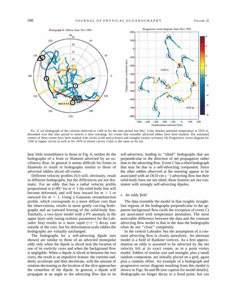
FIG. 9. Potential temperature/salinity diagrams for (a) the cold anticyclones and (b) the warm cyclones, with s1500 contours (contour intervalof 0.01 g kg21). In both panels, the mooring Jun–Nov mean is shown as a thick dashed black line marked by circles, and the shaded regionrepresents the mean plus or minus one standard deviation. The black line is the mean May–Jun 1994 CTD profiles along the WOCE AR7Wline for water depths greater than about 2200 m. In (a), the u/S properties of the eddy cores at 1010 m are given by circled letters. The thickblack line marked by triangles is the mean mooring profile for Mar 1995. In (b), the thin dashed black line is the mean CTD profile fromthe Irminger boundary current on the Greenland side of the Labrador Basin. The mooring profiles through the two warm eddies for the upperfour instruments are shown with thick black lines marked by squares (eddy C) or triangles (eddy D). Mooring instrument depths are 260,510, 1010, 1510, 2010, and 2512 m, with the lowest depth omitted except for the mean profiles.

ically 20.18C at around 500–750 m. Their propertiesare in the approximate range u ; 2.6–2.7, S ; 34.81–38.82 psu. Eddies B, E, and F have apparent radii X ofroughly 5 km so that their true radii are probably com-parable to the deformation radius of 7 km, while eddyA is much larger (X ; 15 km).

A trapping of the eddy currents in the upper 2.5 kmappears to be a general feature of the four anticyclones,with no detectable signal of the eddy currents at thebottom current meter (3476 m). The strong isopycnaldepression (see Fig. 4c) of the stratified lower layerbeneath the eddy core apparently cancels the anticy-clonic flow before it reaches the bottom. Associatedstrong density minima (0.015–0.025 kg m23) observedat 2500 m therefore appear to be a good indication ofsmall-scale anticyclonic eddy activity in the upper layer.In the 1994 CTD section (Fig. 2), two cusplike depres-sions of the deep stratification associated with freshanomalies are probably profiles through cold eddies likethose observed at the mooring. The other cusplike de-pressions with no u/S anomalies may also be due tonearby anticyclones. Similar features are observed inother years.

Rossby number estimates for the anticyclones spanthe range from � ; 0.1 to � ; 0.5, with the two best-observed events (B and F) having relatively high Rossbynumbers (0.25–0.5).

Events C and D are similar to each other in that theyboth have warm, salty u/S anomalies and cyclonic cur-rents. However, event C has a large surface-trapped

bowl of warm, salty water, whereas event D has only aweak and patchy u/S anomaly. These do not match theeddy-advection model as well as the anticyclones. Inparticular, the tilted hodograph of eddy C could meanthat it is part of a self-advecting dipole, and thereforethe size estimate (assuming advection) could be an un-derestimate. Unlike the anticyclones, they both have sig-nificant flow at the bottom. They are at least 12–20 kmradius, substantially larger than the deformation radiusof 7 km, with currents of 10–15 cm s21. Rossby numbersare lower than for the anticyclones, in the range � ;0.1–0.2, owing to the cyclones’ larger size.

b. u/S properties and origin

The u/S properties of the cold anticyclones are shownin Fig. 9a, together with CTD profiles from the centralLabrador Sea during May/June 1994 and the one-stan-dard-deviation envelope of mooring u/S variability dur-ing June–November 1994. The cores of the cold eddiescontain water that is significantly colder (by ;0.05–0.18C) and fresher (by ;0.01–0.02 psu) than the am-bient water. These properties do not match any otherwater masses in the North Atlantic since LSW is alreadycolder and fresher along isopycnals than surroundingwater masses. However, Labrador Sea Water itself un-dergoes an annual cycle in u/S properties (Lazier 1980;LS99). The coldest, freshest waters observed at a givendepth occur as the convective mixed layer passes thatdepth, typically in February–March for depths greater


←

FIG. 10. Details of eddy F. (a, c, e) Time series, offset by an amount proportional to the depth spacing between instruments. Vertical graylines mark the edge of the velocity core, and horizontal gray lines mark the depths of measurements. Note that (a) and (c) have wider timeaxes than (e). (b, d, f ) Vertical profiles, and the vertical gray lines mark the locations of the normal velocity extrema. Horizontal lines againmark the depths of measurements. In (b) and (f ), profiles are shown every 4 h, and thick (thin) lines are for times inside (outside) the eddycore. (a) and (b) The normal velocity y n through the eddy. The perturbation pressure inferred from the velocity data is shown in (c) and (d).The contribution of the geostrophic term fy is the thin line, and the total ( fy 1 y 2r21) is the thick line. Profiles in (d) are through the centerof the eddy. The isopycnal displacement DZs is shown in (e) and (f ).

than 500 m. After deep convection, the water columnbecomes warmer and saltier along isopycnals (by 0.28at 500 m between June and December 1994), apparentlydue to mixing with warm, salty water from the IrmingerCurrent (LS99). Although we have no observations ofu/S properties during March 1994, the u/S propertiesfrom March 1995 were probably comparable (based onone-dimensional mixing applied to the partly restratifiedMay–June CTD sections) and are cold and fresh enoughto account for the u/S properties of the eddies. Therefore,it seems clear that the eddies contain convected waterthat has been insulated from the isopycnal warming andsalinization experienced by the rest of the Labrador Sea.Assuming the eddies were formed around March 1994,we infer that eddies A, B, E, and F are about 3, 4, 5,and 8 months old, respectively.

The u/S diagram for the warm cyclones (Fig. 9b)shows that these eddies are warmer, saltier, and lessdense than the surrounding water, by ;0.1–0.28C,;0.05–0.1 psu, and ;0.02–0.04 g kg21 at ;500 m.CTD casts are also shown from stations in the Irmingerboundary current on the Greenland side of the AR7Wline. The warm eddies are in between the u/S extremesof the boundary current core and the Labrador Sea in-terior, and have identical properties to water from theoffshore edge of the Irminger Current. In contrast, theNorth Atlantic Current (to the southeast of the LabradorSea) contains much more buoyant water, with temper-atures within the same isopycnal band far higher (0.58or more) than those associated with the warm eddies.

A local origin in the Irminger Current is also con-sistent with the potential vorticity structure of the warmeddies. Conservation of potential vorticity states

z 1 f z 1 ff f i i5 , (5)

h hf i

where h is the thickness of an isopycnal layer, z is thevertical relative vorticity, and subscripts i and f denotethe initial and final states of the eddy. The initial large-scale relative vorticity is negligable relative to f (as-suming an 80 cm s21 shear over 50 km). The relativevorticity of the end state can be estimated, assumingsolid-body rotation, as z f 5 2VR21 5 � f f or 0.1–0.2f f . For eddies generated nearby f is approximately con-stant, and we can rewrite (5) as

h 2 hf i5 � , (6)

hi

which means the cyclonic eddies could be explained bya 10%–20% stretching. The warm eddies have u/Sanomalies along isopycnals to a depth of 2000 m (Fig.9b), so the appropriate isopycnal range is between s1.5

5 34.69 and about s1.5 5 34.63. The thickness betweenthese isopycnals increases by about 40% from theboundary current (Fig. 2) to the warm eddies observedat the mooring, which is more than sufficient to accountfor the observed relative vorticity.

c. Detailed structure of an anticyclone

Since eddy F was fortuitously sliced close to its cen-ter, we are able to look at the structure of this event ingreater detail. The vertical structure of the currents andisopycnal displacements associated with eddy F areshown in Figs. 10a–d. As mentioned previously, theflow is nonzero, even at the sea surface, but a middepthmaximum is obvious. However, isopycnal displace-ments decay to zero before reaching the surface; thatis, there are no outcrops associated with the anticyclone.The anticyclonic flow observed near the surface musttherefore be due to an uplift of the sea surface; the sameis true for the other anticyclones.

The magnitude of the sea surface displacement canbe inferred from the momentum equations. The x-in-tegrated x-momentum equation for an azimuthally sym-metric feature located at the origin is

x 2yp9(x) 5 r fy 1 dx9, (7)o E 1 2x90

where p9 is the departure of the pressure field from themotionless hydrostatic state. The estimated advectingflow speed can then be used to substitute U | t 2 to | forx. We find it is necessary to subtract away the stronglylow-passed (240 h) current at each depth so that thepressure signal due to the eddy alone can be isolatedfrom its surroundings. The cyclostrophic term y 2/r isimportant only within about 1/4 radius from the eddycenter (Figs. 10e,f), where it amounts to about a 15%correction to the geostrophic term fy. The pressure fieldis somewhat narrower but stronger at middepths, withthe 110- and 2500 m pressure fields approximately equalin size and magnitude. The magnitude of the high pres-sure region at the surface (100 Pa) is equivalent to a 1cm elevation of the sea surface.

The u/S core of eddy F is not a single lens but has a


composite structure.1 The maximum currents are asso-ciated with a u/S lens near 1 km, above and beneathwhich there are other u/S anomalies. No u/S anomalyis observed at 1.5 km, but at 2 km a lens with u/Sproperties and density similar to the main lens is ob-served. Higher in the water column, a third lens of verydifferent u/S properties is observed, with no distinctvelocity extremum. Its freshness and low density makeit unlikely to have originated in the interior LabradorSea. More likely, it is convectively modified boundarycurrent water. Two other anticyclonic eddies (A and B)show similar, though less pronounced, composite struc-tures.

d. Comparison of the anticyclones with other eddies

To the best of our knowledge, long-lived convectivelyformed eddies have not previously been reported, eitherin the Labrador Sea or elsewhere. Deformation-scaleanticyclones have been observed during active convec-tion in the Labrador Sea (Gascard and Clarke 1983),and it is possible that such eddies eventually evolve intothe anticyclonic eddies we observed 3–8 months fol-lowing the end of deep convection. Similarly eddies ofboth signs have been observed during active convectionin the Mediterranean Sea (Gascard 1978).

The Labrador Sea anticyclones appear to be an ex-ample of a ‘‘submesoscale coherent vortex’’ (SCV) asdefined by McWilliams (1988). In a comparison of anumber of different SCVs from D’Asaro et al. (1994),the range of Rossby numbers for three meddies and twohydrothermal megaplumes is ;0.2–0.6, while the twoArctic Ocean eddies reported have Rossby numbersgreater than 0.6. The range of estimated Rossby numbersfor the cold Labrador Sea eddies (0.1–0.5) makes theanticyclones more similar to meddies and to hydro-thermal megaplumes than to Arctic Ocean eddies. Thisperhaps reflects a common origin: meddies, hydrother-mal megaplumes, and Labrador Sea anticyclones aremost likely all collapse events of some kind, whereasthe Arctic eddies may be generated through lateral fric-tion (D’Asaro 1988).

One distinguishing feature of the anticyclonic eddiesis their strong surface expression. The exact magnitudeof the surface expression of other coherent eddies is stilla matter of debate, but a survey of some meddy literature(Riser et al. 1986; Elliott and Sanford 1986; Kase andZenk 1987; Stammer et al. 1991) suggests that an upperbound on the ratio of surface to maximum flow is one-third, with many potentially having much weaker sur-face expressions. The Labrador Sea anticyclones, bycontrast, typically have a current strength measured at110 m that is one-half the maximum value.

1 Note that this composite structure is not an artifact of interleavingtwo different kinds of temperature instruments (Aanderaas and SEA-CATs) with drastically different accuracy. The cores and the breaksbetween them are all observed by the SEACATs.

The composite nature of the Labrador Sea anticy-clones, most apparent in eddy F (Fig. 5f), is anotherimportant feature. Other observed SCVs tend to have asingle well-defined u/S anomaly in the vertical. This istrue for meddies (Armi and Zenk 1984; Hebert et al.1990; Pingree and LeCann 1993) as well as others (El-liott and Sanford 1986; Riser et al. 1986; D’Asaro etal. 1994), with a notable exception being the doublemeddy observed by Prater and Sanford (1994). Suchcomposite cores may be related to the evolution of bar-oclinic planetary turbulence into a more barotropic state;this effect is seen in layered models (Rhines 1977) aswell as in three-dimensional models (McWilliams et al.1994) of rotating stratified turbulence.

Despite the fact that anticyclonic eddy cores occur atdepths between 500 m and 1500 m, from the point ofview of a two-layer model they represent upper-layerpotential vorticity anomalies. The dynamically impor-tant stratification to the first baroclinic mode is the thickdeep pycnocline beneath 2 km, not the thin surface strat-ification. This is in contrast to many subtropical eddies,which tend to have PV anomalies within or beneath themain pycnocline.

6. Discussion

We identify a number of events observed at the Bravomooring during June–November 1994 as advected ed-dies of two distinct types: two cyclones and four anti-cyclones. Warm cyclones appear to originate in the Ir-minger boundary current, while cold anticyclones areproducts of deep convection.

When compared with other known submesoscale ed-dies, the Labrador Sea anticyclones are characterized bytheir strong barotropic modes and composite cores.Based on their Rossby numbers, the Labrador Sea an-ticyclones appear more closely related to meddies andhydrothermal megaplumes than to Arctic Ocean eddies.

The nature and statistics of the observed eddies areimportant for our understanding of deep convection. Forinstance, in numerical models of deep convection thebaroclinic instability of a convected ‘‘chimney’’ leadsto roughly equal numbers of cyclonic and anticycloniceddies organized into rapidly propagating ‘‘hetons’’(Legg and Marshall 1993; Send and Marshall 1995).Yet, of the six eddies we observed, none are convec-tively generated cyclones; events C and D originate inthe boundary current and not in central Labrador Seadeep convection.

Acknowledgments. Helpful and stimulating commentsfrom the following people are gratefully acknowledged:Eric D’Asaro, Eric Kunze, Mitsuhiro Kawase, CharlieEriksen, Knut Aagaard, Parker MacCready, Jody Kly-mak, and Mark Prater. The vertical mode MATLABcode was cheerfully supplied by Gabe Vecchi and Se-bastian. Hydrographic data was taken during the spring1994 cruise of the C.S.S. Hudson, with John Lazier as


chief scientist. Support for J. Lilly from a NDSEG Grad-uate Student Fellowship was greatly appreciated.

APPENDIX

Estimating the Sizes and Strengths ofAdvected Eddies

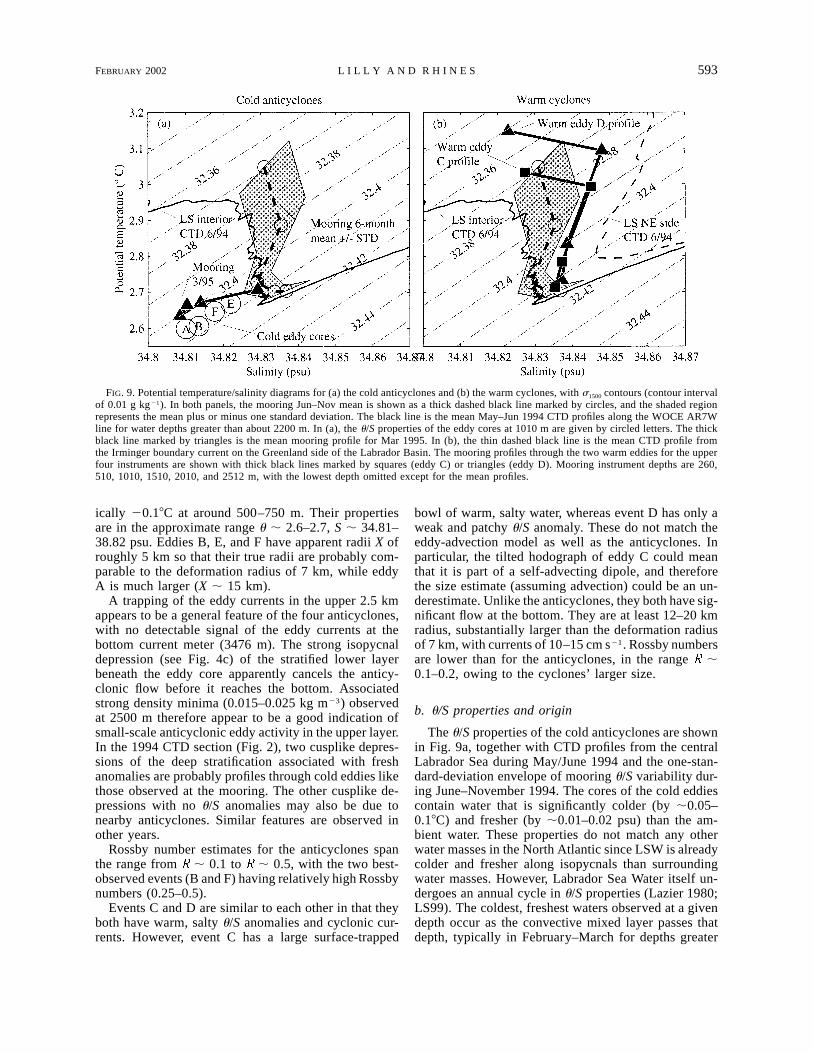
We now define a set of measures used to characterizecoherent eddies. The actual peak azimuthal velocity atany depth is V, the half-width or ‘‘apparent’’ radius isX, and the eddy is moving with a speed U in directionQ. We would like to form estimates of these quantities,denoted V, X, U, and .Q

The edges of an eddy’s velocity core are expected todefine a local maximum of the velocity difference be-tween two points. Given initial guesses for the eddy’scenter to and half-duration DT, refined values are foundthat maximize

V [ | j(t 2 DT) 2 j(t 1 DT) | ,n o o

where j is the complex velocity u 1 iy, over a windowsmall enough to prevent interference from other eddies.Since we also expect the velocity signal to be largestin the direction perpendicular to the advecting flow, theadvection direction (61808) can be estimated as 5Qarg{Vn} 1 p/2.

For a constant background flow advecting an azi-muthally symmetric eddy, Vn will be the velocity com-ponent perpendicular to the advecting flow, which isequivalent to VXR21 where R is the eddy radius and Xis the half-width of the eddy chord intersected by themooring. This measure is expected to underestimate themagnitude of the azimuthal velocity, but has the ad-vantage that aliasing of the advecting flow is minimized.

A second measure of the eddy velocity can be formedby subtracting an estimate of the advecting flow,

1 ˜iQ˜ ˜ wV 5 zj(t 2 DT ) 2 U e zU o w2

1 ˜iQ˜ w1 zj(t 1 DT ) 2 U e z,o w2

where the specific mean flow estimate Uw is defined˜iQwebelow.

The eddy polarity (cyclonic or anticyclonic) is foundfrom the vertical structure of the speed together withthe density structure. Note that Vn and VU are adjustedto be positive for a cyclone and negative for an anti-cyclone.

If the advecting flow is large in magnitude relativeto the eddy, and slowly varying relative to the eddy’sduration, then the advecting flow can be estimated bylow passing the time series. This estimate U f is de-˜iQfefined as the low-passed filtered velocity times series u1 iy at the eddy center t0. The instrument level usedcorresponds to the eddy’s maximum currents, and thefilter is a Hanning window whose width is three timesthe width of the eddy core.

A second way to estimate the advection velocity isto compare the observed currents with the observedshear. For an equivalent barotropic eddy, the eddy cur-rents will be everywhere parallel to the eddy verticalshear. However, the total currents will not be parallel tothe observed shear, since the eddy currents are offsetby the (presumably barotropic) advecting flow but theshear is not. Therefore, the estimate Ua minimizes˜iQaethe angle difference

˜iQ˜ aDQ 5 zarg{j 2 U e } 2 arg{j 2 j }z (A1)z a z zmax max min

over the time window encompassing the eddy, whichwe choose to be (to 2 2DT, to 1 2DT). Here zmax (zmin)is the depth at which the eddy currents are largest (small-est).

These two estimates of the advection flow lead to twocorresponding estimates of the eddy size (Xf and Xa)since UDT 5 X. It should be emphasized that the ap-parent eddy size as observed from the mooring will tendto be smaller than the actual radius, since the eddieswill generally be sliced off-center.

The resulting estimates are shown in Table 2. Agree-ment between the two methods of estimating U is goodexcept for eddy A, which is the longest-duration event.This is encouraging since these two methods are quitedifferent. The two methods for estimating V also agreewell, with only eddy E having a significant differencebetween the two methods.

REFERENCES

Armi, L., and W. Zenk, 1984: Large lenses of highly saline Medi-terranean Water. J. Phys. Oceanogr., 14, 1560–1576.

Clarke, R. A., and J.-C. Gascard, 1983: The formation of LabradorSea Water. Part I: Large-scale processes. J. Phys. Oceanogr., 13,1764–1778.

D’Asaro, E. A., 1988: Generation of submesoscale vortices: A newmechanism. J. Geophys. Res., 93 (C6), 6685–6693.

——, S. Walker, and E. Baker, 1994: Structure of two hydrothermalmegaplumes. J. Geophys. Res., 99 (C10), 20 361–20 373.

Elliott, B., and T. Sanford, 1986: The subthermocline lens D1. PartI: Description of water properties and velocity profiles. J. Phys.Oceanogr., 16, 532–548.

Gascard, J., 1978: Mediterranean deep water formation, baroclinicinstability, and oceanic eddies. Oceanol. Acta, 1, 315–330.

——, and R. A. Clarke, 1983: The formation of Labrador Sea Water.Part II: Mesoscale and smaller-scale processes. J. Phys. Ocean-ogr., 13, 1779–1797.

Hakkinen, S., 1999: A simulation of the effects of a Great SalinityAnomaly. J. Climate, 12, 1781–1795.

Hebert, D., N. Oakey, and B. Ruddick, 1990: Evolution of a Medi-terranean salt lens: Scalar properties. J. Phys. Oceanogr., 20,1468–1483.

Jones, H., and J. Marshall, 1997: Restratification after deep convec-tion. J. Phys. Oceanogr., 27, 2276–2287.

Kase, R. H., and W. Zenk, 1987: Reconstructed Mediterranean saltlens trajectories. J. Phys. Oceanogr., 17, 158–163.

Lazier, J. R. N., 1973: The renewal of Labrador Sea Water. Deep-Sea Res., 20, 341–353.

——, 1980: Oceanographic conditions at Ocean Weather Ship Bravo,1964–1974. Atmos.–Ocean, 18, 227–238.

Legg, S., and J. Marshall, 1993: A heton model of the spreadingphase of open-ocean deep convection. J. Phys. Oceanogr., 23,1040–1056.


——, J. McWilliams, and J. Gao, 1998: Localization of deep oceanconvection by a mesoscale eddy. J. Phys. Oceanogr., 28, 944–970.

Lilly, J. M., P. B. Rhines, M. Visbeck, R. Davis, J. R. Lazier, F.Schott, and D. Farmer, 1999: Observing deep convection in theLabrador Sea during winter 1994/95. J. Phys. Oceanogr., 29,2065–2098.

Marshall, J., and F. Schott, 1999: Open-ocean convection: Obser-vations, theory and models. Rev. Geophys., 37, 1–64.

McWilliams, J. C., 1988: Vortex generation through balanced ad-justment. J. Phys. Oceanogr., 18, 1178–1192.

——, J. B. Weiss, and I. Yavneh, 1994: Anisotropy and coherentvortex structures in planetary turbulence. Science, 264, 410–413.

Pingree, R., and B. LeCann, 1993: Structure of a Meddy (Bobby 92)southeast of the Azores. Deep-Sea Res., 40, 2077–2103.

Prater, M. D., and T. Sanford, 1994: A Meddy off Cape Vincent. PartI: Description. J. Phys. Oceanogr., 24, 1572–1586.

Rhines, P. B., 1977: The dynamics of unsteady currents. The Sea, E.Goldberg, Ed., Marine Modeling, Vol. 6, John Wiley and Sons,189–318.

Riser, S. C., W. B. Owens, H. T. Rossby, and C. C. Ebbesmeyer, 1986:The structure, dynamics, and origin of a small-scale lens of waterin the western North Atlantic thermocline. J. Phys. Oceanogr.,16, 572–590.

Send, U., and J. Marshall, 1995: Integral effects of deep convection.J. Phys. Oceanogr., 25, 855–872.

Stammer, D., H.-H. Hinrichsen, and R. H. Kase, 1991: Can Meddiesbe detected by satellite altimetry? J. Geophys. Res., 96 (C4),7005–7014.

Straneo, F., and M. Kawase, 1999: Comparisons of localized con-vection due to localized forcing and preconditioning. J. Phys.Oceanogr., 29, 55–68.

Talley, L., and M. McCartney, 1982: The distribution and circulationof Labrador Sea Water. J. Phys. Oceanogr., 12, 1189–1205.

102 3&( 545 6

Documents

Transcript of 102 3&( 545 6