0&%'$(&1)213&,.&4(5,) 6$+7$'8)9($.:);($%'&();(& - core.ac.uk · Pelo teorema de Darboux existe...
104
Universidade de Lisboa Faculdade de Ciências Departamento de Matemática Legendrian Varieties and Quasi‐Ordinary Hypersurfaces António Manuel Bandeira Barata Alves de Araújo Doutoramento em Matemática Geometria e Topologia 2011
Transcript of 0&%'$(&1)213&,.&4(5,) 6$+7$'8)9($.:);($%'&();(& - core.ac.uk · Pelo teorema de Darboux existe...

UniversidadedeLisboa
FaculdadedeCiências
DepartamentodeMatemática
LegendrianVarietiesandQuasi‐OrdinaryHypersurfaces
AntónioManuelBandeiraBarataAlvesdeAraújo
DoutoramentoemMatemática
GeometriaeTopologia
2011


UniversidadedeLisboa
FaculdadedeCiências
DepartamentodeMatemática
LegendrianVarietiesandQuasi‐OrdinaryHypersurfaces
AntónioManuelBandeiraBarataAlvesdeAraújo
TeseOrientadapeloProf.DoutorOrlandoManuelBartolomeuNeto
DoutoramentoemMatemática
GeometriaeTopologia
2011


Acknowledgements
I would like to thank, first of all, my PhD supervisor, Prof. Orlando Neto,
not only for all he valiantly tried to teach me about mathematics, but also
and above all else for putting up with my unfailing ability to get hopelessly
distracted by this and that enthusiasm over the years.
A big thank you to my colleague Joao Cabral, for trying to teach me about
the combinatorics of blow ups, and for not exploding in the attempt.
I have to thank my colleagues at Universidade Aberta, for keeping my teach-
ing duties within reasonable bounds at a time of big change (and inevitably
some shared toil and turmoil) at our University.
I would like to thank my close friends, but I wouldn’t know what order
to choose, or if they even are in any meaningful way a totally ordered set
(lexycographic is diplomatic but somehow cold); so I’ll just say you know
who you are and where you stand in my thoughts (especially you who would
blush if mentioned at the top of the list) and leave it at that .
Like so many through the ages, fully acknowledging the cliche and the deep
reasons that justify it, I’d like to thank my parents, for all the same good
reasons for which so many people thank their parents in PhD thesis acknowl-
edgments. Mother won’t mind if I especially thank my dear father, who can
no longer be with us, but who my mind still often conjures up in my dreams,
to give me good advice that I often fail to follow. Thanks anyway, Dad!...
I like to hear it even if I then go out and foolishly do my own thing. This
thesis (for what that may be worth) is dedicated to you.
(next one’s yours, Mom!).
This work was financially supported by Fundacao para a Ciencia e
Tecnologia, Portugal, through a PhD scholarship with reference PRAXIS
XXI/BD/15915/98.

Resumo
Dada uma variedade X de dimensao 2n+1, chama-se forma de contacto de
X a uma forma diferencial ω de grau 1 tal que ω(dω)n = ω ∧ dω ∧ · · · ∧ dωe nao-nula em todos os pontos. Pelo teorema de Darboux existe localmente
um sistema de coordenadas (x1, . . . , xn, p1, . . . , pn−1) tal que ω = dxn −∑n−1i=1 pidxi. Seja L um OX -modulo do feixe das formas diferenciais de grau
1, Ω1X . O feixe L diz-se uma estructura de contacto sobre X se para todo o
o ∈ X existe uma forma de contacto ω definida numa vizinhanca aberta U
de o tal que L |U = OXω. O par (X,L) diz-se uma variedade de contacto.
A geometria de contacto e o equivalente em dimensao ımpar da geome-
tria simplectica. Seja Γ um subconjunto analıtico de uma variedadede de
contacto (X,L) de dimensao 2n − 1. O conjunto Γ diz-se uma variedade
Legendriana se Γ tem dimensao n− 1 e a restricao a parte regular de Γ de
qualquer seccao ω de L se anula identicamente. Uma variedade Legendriana
e o equivalente em geometria de contacto a uma variedade Lagrangeana em
Geometria Simpletica.
Dada uma variedade complexa X de dimensao n, o fibrado cotangente T ∗X
de X esta munido de uma forma diferencial θ de grau 1, a forma canonica
de T ∗X. Vamos denotar por π a projeccao de T ∗X sobre X. A forma dθ
e uma forma simplectica de T ∗X. Na verdade dθn e nao-nula em todos os
pontos. O fibrado projective cotangente P∗X tem uma estructura canonica
de variedade de contacto. Se X = Cn, T ∗X = Cn × Cn onde Cn representa
o dual de Cn. Se considerarmos em Cn as coordenadas (x1, . . . , xn) e em Cn
as coordenadas duais (ξ1, . . . , ξn), θ =∑n
i=1 ξidxi, e dθ =∑n
i=1 dξidxi.
Entao P∗Cn = Cn × Pn, onde Pn denota o espaco projectivo de Cn. Temos
que P∗Cn e a uniao dos abertos Ui = ξi 6= 0, 1 ≤ i ≤ n. Temos em Ui
o sistema de coordenadas (x1, . . . , xn,ξ1ξi, . . . , ξi−1
ξi, ξi+1
ξi, . . . , ξn
ξi). A forma de
contacto ωj =θ
ξj= dξj +
∑j 6=i
ξi
ξjdxi e uma forma de contacto sobre Ui. As
formas diferenciais ωi, 1 ≤ i ≤ n, determinam uma estructura de contacto
L sobre P∗Cn.
Dada uma hipersuperfıcie S = f = 0 sobre um aberto de Cn, temos uma
aplicacao
a 7→(∂f
∂x1(a) : · · · : ∂f
∂xn(a))
i

definida sobre a parte regular de S com valores em Pn. O fecho em P∗Cn
do grafico desta aplicacao diz-se o conormal de S. O conormal de S e
uma variedade Legendriana de P∗Cn. Dado um ponto a ∈ S, o conjunto
Σ = Γ ∩ π−1(a) diz-se o limite de tangentes de S no ponto a.
Seja (S, o) um germe de hipersuperfıcie de uma variedade complexa X
definido por um germe de funcao holomorfa f ∈ OX,o. Dizemos que (S, o)
e uma hipersuperfıcie quasi-ordinaria se existe um sistema de coordenadas
locais (x1, . . . , xn) centrado em o tal que a imagem pela aplicacao
(x1, . . . , xn) 7→ (x1, . . . , xn−1) (0.0.1)
do conjunto f =
∂f
∂xn= 0
(0.0.2)
e igual a
x1 · · ·xx = 0. (0.0.3)
O conjunto (0.0.2) diz-se o contorno aparente de S relativamente a projeccao
(0.0.1) e o conjunto (0.0.3) diz-se o discriminante de S relativamente a
projeccao (0.0.1).
A singularidade quasi-ordinaria caracteriza-se pelo facto de admitir parame-
trizacoes em series de potencias fracionarias do tipo
xn = ϕ(x1, . . . , xn−1). (0.0.4)
Toda a curva (hipersuperfıcie de uma variedade de dimensao 2) e uma
superfıcie quasi-ordinaria. Newton foi o primeiro a descobrir que toda a
curva complexa admite uma parametrizacao do tipo (0.0.4), normalmente
chamada de expansao de Puiseux.
O objectivo central desta tese e o estudo das variedades Legendrianas que
sao conormais de hipersuperfıcies quasi-ordinarias.
O primeiro capıtulo dedica-se ao estudo das curvas Legendrianas. O re-
sultado fundamental e um teorema de classificacao de curvas Legendrianas.
Trata-se de uma versao para curvas Legendrianas de um teorema de Delorme
(ver [7]) para curvas planas. Mostra-se que o conjunto das curvas Legendri-
anas que verificam uma condicao de genericidade associada ao semigrupo da
curva formam um aberto de Zariski de um espaco projectivo pesado.
ii

Um dos instrumentos fundamentais para a prova do teorema consiste num
teorema que descreve todas as transformacoes de contacto de uma variedade
de contacto de dimensao tres. Consideramos em (C3, 0) a estructura de
contacto definida pela forma de contacto dy−pdx. toda a transformacao de
contacto cuja derivada deixe invariante a recta y = p = 0 e a composicao
de transformacoes do tipo
(x, y, p) 7→ (λx, µy,µ
λp) (0.0.5)
e
(x, y, p) 7→ (x+ α, y + β, p+ γ) (0.0.6)
onde α, β, γ pertencem ao ideal maximal do anel Cx, y, p. Dados α ∈Cx, y, p e β0 ∈ Cx, y, temos que β e solucao do problema de Cauchy
∂β
∂x− (p+ γ)
(1 +
∂α
∂x+ p
∂α
∂y
)+ p
(1 +
∂β
∂y
)= 0,
com β − β0 ∈ (p). Alem disso,
γ =(
1 +∂α
∂x+ p
∂α
∂y
)−1(∂β∂x
+ p
(∂β
∂y− ∂α
∂x− p∂α
∂y
)).
Temos que toda a transformacao de contacto de (C3, 0) em (C3, 0) e a com-
posicao de transformacoes do tipo (0.0.5), (0.0.6) e uma transformacao de
contacto paraboloidal (ver [11])
(x, y, p) 7→ (ax+ bp, y − 12acx2 − 1
2bdp2 − bcxp, cx+ dp),
∣∣∣∣∣ a b
c d
∣∣∣∣∣ = 1.
O teorema de classificacao de transformacoes de contacto referido acima e
talvez o mais importante resultado de [1], tendo ja sido citado em [6]. E
tambem citado em dois outros trabalhos actualmente em preparacao.
Como consequencia do teorema fundamental deste capıtulo, e possıvel clas-
sificar explıcitamente em muitas situacoes todas as curvas Legendrianas que
sao os conormais de uma curva plana com um unico par de Puiseux (p, q).
O segundo capıtulo desta tese dedica-se ao estudo dos limites de tangentes
de uma hipersuperfıcie quasi-ordinaria. Podemos encontrar a solucao deste
problema num caso muito particular em [2].
iii
Uma das consequencias fundamentais deste resultado e mostrar que, sempre
que o cone tangente de uma hipersuperfıcie quasi-ordinaria e um hiperplano,
o limite de tangentes e um invariante topologico da hipersuperfıcie.
Este resultado leva-nos a perguntar se podemos esperar que, quando o cone
tangente de uma hipersuperfıcie arbitraria e um hiperplano, o limite de
tangentes e um invariante topologico da hipersuperfıcie.
No terceiro capıtulo da tese aplica-se o resultado fundamental do segundo
capıtulo ao estudo do comportamento por explosao do conormal de uma
hipersuperfıcie quasi-ordinaria. Obtemos desta forma um teorema de res-
olucao de singularidades para superfıcies Legendrianas que sao conormais
de superfıcies quasi-ordinarias.
Seja π : X → X uma explosao de uma variedade de contacto X com um
centro dado D. Dada uma estructura de contacto L em X nao podemos
esperar que exista em X uma estructura de contacto L para a qual π e uma
transformacao de contacto. Na verdade toda a transformacao de contacto
e bijectiva, e π so e bijectiva se D = ∅. Neto mostrou em [18] que existe
uma nocao de variedade de contacto logaritmica que generaliza a nocao de
variedade de contacto. Dada uma variedade Legendriana lisa Λ de X, o
blow up X de X com centro Λ tem uma estructura de variedade de contacto
logaritmica com polos ao longo do divisor excepcional de π. As seccoes
do fibrado cotangente T ∗M sao as formas diferenciais de grau 1 que sao
as seccoes do feixe Ω1M . Dado um divisor com cruzamentos normais N de
M , vamos denotar por Ω1M 〈N〉 o feixe das formas diferenciais logaritmicas
de grau 1 com polos em N . Vamos chamar fibrado cotangente logaritmico
ao fibrado T ∗〈M/N〉 cujo feixe de seccoes e Ω1M 〈N〉. Vamos denotar por
P∗〈M/N〉 a projectivizacao do fibrado T ∗〈M/N〉.Seja L uma subvariedade lisa de M tal que para toda a componente irre-
dutıvel Ni de N , L esta contida em Ni ou L e transversal a Ni. Podemos
definir PL〈M/N〉 de forma semelhante a usada para definir PLM .
O resultado seguinte e um dos instrumentos essenciais na prova do teorema
fundamental deste capıtulo.
Theorem 0.0.1. (i) Seja (X,L) uma variedade de contacto logarıtmica com
polos ao longo de Y . Seja Λ uma subvariedade Legendriana bem comportada
iv

de X. Seja τ : X → X o blow up de X ao longo de Λ. Seja E = τ−1(Λ).
Entao O eX-module O eX (E)τ∗L e uma estructura de contacto logarıtmica em
X com polos ao longo de τ−1(Y ).
(ii) Seja M uma variedade e N um divisor com cruzamentos normais de M .
Seja L uma subvariedade bem comportada de M . O conormal Λ = P∗LM de
L e uma subvariedade Legendriana bem comportada de P ∗〈M/N〉. Seja
ρ : M → M o blow up de M ao longo de L. Seja E = ρ−1(L). Seja
N = ρ−1(N). Entao existe uma transformacao de contacto injectiva ϕ de
um subconjunto aberto denso Ω do blow up X de P ∗〈M/N〉 ao longo de Λ
para P ∗〈M/N〉 tal que o diagrama (0.0.7) comuta.
P ∗〈M/N〉 τ← X ← Ωϕ→ P ∗〈M/N〉
π ↓ ↓ πM
ρ←− M
(0.0.7)
(iii) Seja M uma variedade e N um divisor com cruzamentos normais de M .
Seja L uma subvariedade bem comportada de (M,N). Seja σ a projeccao
canonica de TΛP∗〈M/N〉 sobre TLM . Seja S um germe de um subconjunto
analıtico natural de (M,N) em o ∈ N . Seja Γ = P∗S〈M/N〉. Se S tem limite
de tangentes trivial em o, entao Γ ∩ π−1(o) = λ e CΛ(Γ) ∩ σ−1(L) ⊂ Λ,
Γ ⊂ Ω e ϕ(Γ) = P∗eS〈M/N〉.
A prova do Teorema de resolucao de singularidades depende de um argu-
mento combinatorio baseado no algoritmo de resolucao de singularidades
para superfıcies quasi-ordinarias.
Palavras chave: Espacos de Moduli; Geometria Algebrica; Hipersuperfıcie
quasi-ordinaria; Limites de tangentes; Teoria das singularidades; Variedade
de contacto; Variedade Legendriana.
v


Abstract
This thesis is a study of the Legendrian Varieties that are conormals of
quasi-ordinary hypersurfaces.
In the first chapter we study the analytic classification of the Legendrian
curves that are the conormal of a plane curve with a single Puiseux pair.
Let χm,n be the set of Legendrian curves that are the conormal of a plane
curve with a Puiseux pair (m,n), where g.c.d.(m,n) = 1 and m > 2n, with
semigroup as generic as possible. We show that the quotient of χm,n by
the group of contact transformations is a Zariski open set of a weighted
projective space.
The main tool used in the proof of this theorem is a classification/construction
theorem for contact transformation that has since proved useful in other in-
stances.
In the second chapter we calculate the limits of tangents of a quasi-ordinary
hypersurface. In particular, we show that the set of limits of tangents is, in
general, a topological invariant of the hypersurface.
In the third chapter we prove a desingularization theorem for Legendrian
hypersurfaces that are the conormal of a quasi-ordinary hypersurface. One
of the main ingredients of the proof is the calculation of the limits of tangents
achieved in chapter two.
Keywords: Algebraic Geometry; Contact Variety; Legendrian Variety;
Limits of tangents; Moduli Spaces; Quasi-ordinary Hypersurface; Singu-
larity theory.


Contents
1 Moduli of Germs of Legendrian Curves 3
1.1 Introduction . . . . . . . . . . . . . . . . . . . . . . . . . . . . 5
1.2 Plane curves versus Legendrian curves . . . . . . . . . . . . . 5
1.3 Infinitesimal Contact Transformations . . . . . . . . . . . . . 10
1.4 Examples . . . . . . . . . . . . . . . . . . . . . . . . . . . . . 15
1.5 The generic semigroup of an equisingularity class of irreducible
Legendrian curves . . . . . . . . . . . . . . . . . . . . . . . . 16
1.6 The moduli . . . . . . . . . . . . . . . . . . . . . . . . . . . . 20
2 Limits of tangents of quasi-ordinary hypersurfaces 23
2.1 Introduction . . . . . . . . . . . . . . . . . . . . . . . . . . . . 25
2.2 Limits of tangents . . . . . . . . . . . . . . . . . . . . . . . . 29
3 Desingularization of Legendrian Varieties 47
3.1 Introduction . . . . . . . . . . . . . . . . . . . . . . . . . . . . 49
3.2 Logarithmic differential forms . . . . . . . . . . . . . . . . . . 50
3.3 Logarithmic symplectic manifolds . . . . . . . . . . . . . . . . 52
3.4 Legendrian Varieties . . . . . . . . . . . . . . . . . . . . . . . 59
3.5 Blow up and deformation of the normal cone . . . . . . . . . 62
3.6 Blow ups . . . . . . . . . . . . . . . . . . . . . . . . . . . . . 66
3.7 Resolution of quasi-ordinary surfaces . . . . . . . . . . . . . . 70
3.8 Resolution of Legendrian surfaces . . . . . . . . . . . . . . . . 73


Chapter 1
Moduli of Germs of
Legendrian Curves
In this chapter We construct the generic component of the moduli space of
the germs of Legendrian curves with generic plane projection topologicaly
equivalent to a curve yn = xm.
3


1.1 Introduction
Zariski [23] initiated the construction of the moduli of plane curve singu-
larities. Delorme [7] organized in a systematic way the ideas of Zariski,
obtaining general results o the case of curves with one characteristic expo-
nent in the generic case (see also [20]). Greuel, Laudal and Pfister (see the
bibliography of [8]) stratified the space versal deformations of plane curves,
constructing moduli spaces on each stratum.
In this chapter we initiate the study of the moduli of Legendrian curve sin-
gularities. We construct the moduli space of generic irreducible Legendrian
singularities with equisingularity type equal to the topological type of the
plane curve yn = xm, (n,m) = 1. Our method is based on the analysis of
the action of the group of infinitesimal contact transformations on the set
of Puiseux expansions of the germs of plane curves.
In section 2 we associate to each pair of positive integers n,m such that
(n,m) = 1 a semigroup Γ(n,m). We show that the semigroup of a generic
element of this equisingularity class equals Γ(n,m). In section 3 we classify
the infinitesimal contact transformations on a contact threefold and study
its action on the Puiseux expansion of a plane curve. In section 4 we discuss
some simple examples of moduli of germs of Legendrian curves. In section 5
we show that the generic components of the moduli of germs of Legendrian
curves with fixed equisingularity class are the points of a Zariski open subset
of a weighted projective space.
1.2 Plane curves versus Legendrian curves
Let Λ be the germ at o of an irreducible space curve. A local parametrization
ı : (C, 0) → (Λ, o) defines a morphism ı∗ from the local ring OΛ,o into its
normalization Ct. Let v : OΛ,o → Z ∪ ∞ be the map g 7→ order(ı∗(g)).
We call v(g), g ∈ OΛ,o, the valuation of g. We call Γ = v(OΛ,o) the semigroup
of the curve Λ. There is an integer k such that l ∈ Γ for all l ≥ k. The
smallest integer k with this property is denoted by c and called the conductor
of Γ.
5

Let C be the germ at the origin of a singular irreducible plane curve C
parametrized by
x = tn, y =∞∑
i=m
aiti, (1.2.1)
with am 6= 0 and (n,m) = 1. The pair (n,m) determines the topological
type of C (see for instance [5]).
Example 1.2.1. A monomial space curve is a curve defined by a parametriza-
tion of the type t 7→ (x, y, p) = (a1tn, a2t
m, a3ts), ai ∈ C∗. Let C be
a monomial space curve. The semigroup of any space curve includes the
valuations of all the monomials xiyjpk, i, j, k ∈ N0, which are equal to
order(ι∗(xiyjpk)) = order(tintjmtks) = in + jm + sk. Hence Γ ⊇ in +
jm + ks, i, j, k ∈ N0. Since C is a monomial curve, if u, v are monomials
of OΛ,o, and a, b ∈ C, then order(ι∗(au+ bv)) = min(order(u), order(v)), or
ι∗(au+bv) = 0. Hence, for a monomial curve Γ = in+jm+ks, i, j, k ∈ Z+.The same result applies to monomial plane curves as a particular case, with
the obvious modifications.
Example 1.2.2. Let C be the germ of plane curve germ defined at the
origin of C2 by y3 − x11 = 0. Let ι be the parametrization of C defined by
t 7→ (t3, t11). Then v(xiyj) = order(ι∗(xiyj)) = order(t3i+11j) = 3i + 11j
and, since C is a monomial curve, the semigroup Γ of C is equal to the set
of all such orders for i, j ∈ N0.
It is useful to represent the semigroup of a curve in a table with v(x) columns,
where each place (i, j) of the table represents the valuation iv(x) + j. In
each place of the table we display a monomial that has the corresponding
valuation. Once a monomial u is placed in the table we know that all places
below that monomial along the same column are also in the semigroup, since
moving down one line along a fixed column corresponds to multiplying u by
powers of x. Hence we omit displaying all monomials in (x), except for x
itself. In the current example, we obtain the table (1.1).
Hence, it is easy to see that in this case the semigroup equals
Γ = 3, 6, 9, 11, 12, 14, 15, 17, 18, 20, 21, 22 . . .
In particular, the conductor is c = 20. In general, c = (n− 1)(m− 1) for a
plane curve t 7→ (tn, tm +∑
i>m aiti) such that (n,m) = 1.
6

0 1 2
0
3 x
6 .
9 . y
12 . .
15 . .
18 . .
21 . y2 .
Table 1.1: Semigroup table of Cx, y/(y3 − x11)
Example 1.2.3. Let Λ be the space curve defined in C3x,y,p by the ideal (y3−
x11, y−(3/11)px). A parametrization of Γ is given by ι(t) = (t3, t11, (11/3)t8).
The semigroup is equal to the set of valuations v(xiyjpk), i, j, k ∈ N0. The
semigroup table is
0 1 2
0
3 x
6 . p
9 . y
12 . .
15 . p2 .
18 . py .
21 . y2 .
Table 1.2: Semigroup table of Cx, y, p/(y3 − x11, y − (3/11)px)
Hence the semigroup is the union of 3, 6, 8, 9 with all the integers greater
or equal to 11 except for 13, and the conductor is c = 14.
Example 1.2.4. Consider the family of plane curves defined by t 7→ (t3, t11+∑i>11 ait
i), ai ∈ C. Since (3, 11) = 1, c = (3 − 1)(11 − 1) = 20, and for
k < c, there is at most one monomial with valuation k (the smallest k
7
where two monomials coincide is v(x11) = v(y3) = 33). Hence we still have
Γ = v(xiyj), i, j ∈ N0, and the semigroup table is the same as in example
(1.2.2).
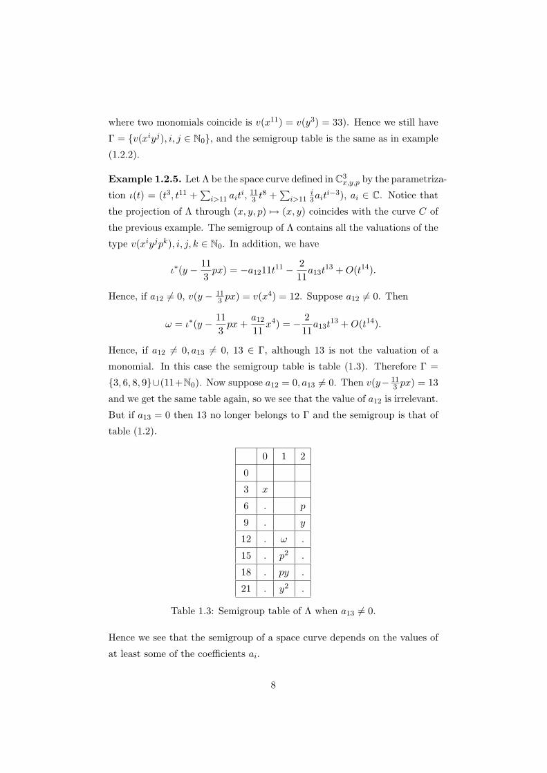
Example 1.2.5. Let Λ be the space curve defined in C3x,y,p by the parametriza-
tion ι(t) = (t3, t11 +∑
i>11 aiti, 11
3 t8 +
∑i>11
i3ait
i−3), ai ∈ C. Notice that
the projection of Λ through (x, y, p) 7→ (x, y) coincides with the curve C of
the previous example. The semigroup of Λ contains all the valuations of the
type v(xiyjpk), i, j, k ∈ N0. In addition, we have
ι∗(y − 113px) = −a1211t11 − 2
11a13t
13 +O(t14).
Hence, if a12 6= 0, v(y − 113 px) = v(x4) = 12. Suppose a12 6= 0. Then
ω = ι∗(y − 113px+
a12
11x4) = − 2
11a13t
13 +O(t14).
Hence, if a12 6= 0, a13 6= 0, 13 ∈ Γ, although 13 is not the valuation of a
monomial. In this case the semigroup table is table (1.3). Therefore Γ =
3, 6, 8, 9∪(11+N0). Now suppose a12 = 0, a13 6= 0. Then v(y− 113 px) = 13
and we get the same table again, so we see that the value of a12 is irrelevant.
But if a13 = 0 then 13 no longer belongs to Γ and the semigroup is that of
table (1.2).
0 1 2
0
3 x
6 . p
9 . y
12 . ω .
15 . p2 .
18 . py .
21 . y2 .
Table 1.3: Semigroup table of Λ when a13 6= 0.
Hence we see that the semigroup of a space curve depends on the values of
at least some of the coefficients ai.
8

Let M be a complex manifold of dimension n. The cotangent bundle πM :
T ∗M → M of M is endowed of a canonical 1-form θ. The differential
form (dθ)∧n never vanishes on M . Hence dθ is a symplectic form on T ∗M .
Given a system of local coordinates (x1, . . . , xn) on an open set U of X,
there are holomorphic functions ξ1, . . . , ξn on π−1M (U) such that θ |π−1
M (U)=
ξ1dx1 + · · ·+ ξndxn.
Let X be a complex threefold. Let ΩkX denote the sheaf of differential
forms of degree k on X. A local section of Ω1X is called a contact form if
ω ∧ dω never vanishes. Let L be a subsheaf of the sheaf Ω1X . The sheaf
L is called a contact structure on X if L is locally generated by a contact
form. A pair (X,L), where L is a contact structure on X, is called a contact
threefold. Let (Xi,Li), i = 1, 2, be two contact threefolds. A holomorphic
map ϕ : X1 → X2 is called a contact transformation if ϕ∗L2 = L1.
Let P∗C2 = C2 × P1 = (x, y, (ξ : η)) : x, y, ξ, η ∈ C, (ξ, η) 6= (0, 0) be
the projective cotangent bundle of C2. Let π : P∗C2 → C2 be the canonical
projection. Let U and V be the open sets of P∗C2 defined respectively by
η 6= 0 and ξ 6= 0. Set p = −ξ/η, q = −η/ξ. The sheaf L defined by
L |U = OU (dy − pdx) and L |V = OV (dx − qdy) is a contact structure on
P∗C2. By the Darboux theorem every contact threefold is locally isomorphic
to (U,OU (dy−pdx)). We call infinitesimal contact transformation to a germ
of a contact transformation Φ : (U, 0) 7→ (U, 0).
A curve Λ on a contact manifold (X,L) is called Legendrian if the restriction
of ω to the regular part of Λ vanishes for each section ω of L. Let C = f =
0 be a plane curve. Let Λ be the closure on P∗C2 of the graph of the Gauss
map G : a ∈ C : df(a) 6= 0 → P1 defined by G(a) = 〈df(a)〉. The set
Λ is a Legendrian curve. We call Λ the conormal of the curve C. If C is
irreducible and parametrized by (1.2.1) then Λ is parametrized by
x = tn, y =∞∑
i=m
aiti, p =
dy
dx=
∞∑i=m
i
nait
i−n. (1.2.2)
Given a Legendrian curve Λ of P∗C2 such that Λ does not contain any fibre
of π, π(Λ) is a plane curve. Moreover, Λ equals the conormal of π(Λ) (see
[21]).
Let (X,L) be a contact threefold. A holomorphic map ϕ : (X, o)→ (C2, 0)
9

is called a Legendrian map if Dϕ(o) is surjective and the fibers of ϕ are
smooth Legendrian curves. The map ϕ is Legendrian if and only if there is a
contact transformation ψ : (X, o)→ (P∗C2, (0, 0, (0 : 1)) such that ϕ = πψ.
Let (Λ, o) be a Legendrian curve of X. Let Co(Λ) be the tangent cone of Λ
at o. We say that a Legendrian map ϕ : (X, o)→ (C2, 0) is generic relatively
to (Λ, o) if it verifies the transversality condition Toϕ−1(0) ∩ Co(Λ) = 0.
We say that a Legendrian curve (Λ, o) of P∗C2 is in strong generic position
if π : (P∗C2, o) → (C2, π(o)) is generic relatively to (Λ, o). The Legendrian
curve Λ parametrized by (1.2.2) is in strong generic position if and only
if m ≥ 2n + 1. Given a Legendrian curve (Λ, o) of a contact threefold X
there is a contact transformation ψ : (X, o)→ (P∗C2, (0, 0, (0 : 1)) such that
(ψ(Λ), o) is in strong generic position (cf [10], section 1).
Example 1.2.6. Let C be the germ of plane curve y2−x3 = 0. The tangent
cone of C is obtained by considering the deformation to the tangent cone
map,
λ 7→ (λ2y2 − λ3x3)λ2
= y2 − λx3,
and setting λ = 0. Hence the tangent cone of C is y = 0.Let Λ be the conormal of C. Λ is the curve parametrized by
t 7→ (x, y, p) = (t2, t3, (3/2)t),
hence Λ verifies the equations y2 − x3 = 0, p2 − (9/4)x = 0. From the first
equation, the tangent cone is contained in y = 0. from the second we get
λp2− (9/4)x = 0, hence x = 0. Hence the tangent cone of Λ is x = y = 0,therefore Λ is not in strong generic position.
We say that two germs of Legendrian curves are equisingular if their images
by generic Legendrian maps have the same topological type.
1.3 Infinitesimal Contact Transformations
Let m be the maximal ideal of the ring Cx, y, p. Let G denote the group of
infinitesimal contact transformations Φ such that the derivative of Φ leaves
invariant the tangent space at the origin of the curve y = p = 0. Let J
10

be the group of infinitesimal contact transformations
(x, y, p) 7→ (x+ α, y + β, p+ γ) (1.3.1)
such that α, β, γ, ∂α/∂x, ∂β/∂y, ∂γ/∂p ∈ m. Set H = Ψλ,µ : λ, µ ∈ C∗,where
Ψλ,µ(x, y, p) =(λx, µy,
µ
λp). (1.3.2)
Let P denote the group of paraboloidal contact transformations (see [11])
(x, y, p) 7→ (ax+bp, y−12acx2−1
2bdp2−bcxp, cx+dp),
∣∣∣∣∣ a b
c d
∣∣∣∣∣ = 1. (1.3.3)
The contact transformation (1.3.3) belongs to G if and only if c = 0. The
paraboloidal contact transformation
(x, y, p) 7→ (−p, y − xp, x) (1.3.4)
Is called the Legendre transformation.
Theorem 1.3.1. The group J is an invariant subgroup of G. Moreover,
the quotient G/J is isomorphic to H.
Proof. . If H ∈ H and Φ ∈ J , HΦH−1 ∈ J . Hence it is enough to show
that each element of G is a composition of elements of H and J . Let Φ ∈ Gbe the infinitesimal contact transformation (x, y, p) 7→ (x′, y′, p′). There is
ϕ ∈ Cx, y, p such that ϕ(0) 6= 0 and
dy′ − p′dx′ = ϕ(dy − pdx). (1.3.5)
Composing Φ with H ∈ H we can assume that ϕ(0) = 1. Let Φ be the germ
of the symplectic transformation (x, y, p; η) 7→ (x′, y′,−ηp′;ϕ−1η). Notice
that Φ(0, 0; 0, 1) = (0, 0; 0, 1). Since DΦ(0, 0; 0, 1) leaves invariant the linear
subspace µ generated by (0, 0; 0, 1), DΦ(0, 0; 0, 1) induces a linear symplectic
transformation on the linear symplectic space µ⊥/µ. There is a paraboloidal
contact transformation P such that DP (0, 0; 0, 1) equals DΦ(0, 0; 0, 1) on
µ⊥/µ. Since D(P−1Φ)(0, 0; 0, 1) induces the identity map on µ⊥/µ, P−1Φ
is an infinitesimal contact transformation of the type (x, y, p) 7→ (x+α, y′, p+
γ), where∂α
∂x,∂α
∂p,∂γ
∂x,∂γ
∂p∈ m. (1.3.6)
11

Set β = y′ − y. It follows from (1.3.5) and (1.3.6) that (∂β/∂y)(0) = 0.
Hence P−1Φ ∈ J . Since Φ and P−1Φ ∈ G, P ∈ G. Therefore p is the
composition of an element of H and an element of J .
Theorem 1.3.2. Let α ∈ Cx, y, p, β0 ∈ Cx, y be power series such that
α, β0,∂β0
∂y∈ m. (1.3.7)
There are β, γ ∈ Cx, y, p such that β−β0 ∈ (p), γ ∈ m and α, β, γ define an
infinitesimal contact transformation Φα,β0 of type (1.3.1). The power series
β and γ are uniquely determined by these conditions. Moreover, (1.3.1)
belongs to J if and only if
∂α
∂x,∂β0
∂x,∂2β0
∂x∂p∈ m. (1.3.8)
The function β is the solution of the Cauchy problem(1 +
∂α
∂x+ p
∂α
∂y
)∂β
∂p− p∂α
∂p
∂β
∂y− ∂α
∂p
∂β
∂x= p
∂α
∂p. (1.3.9)
with initial condition β − β0 ∈ (p).
Proof. . The map (1.3.1) is a contact transformation if and only if there is
ϕ ∈ Cx, y, p such that ϕ(0) 6= 0 and
d(y + β)− (p+ γ)d(x+ α) = ϕ(dy − pdx). (1.3.10)
The equation (1.3.10) is equivalent to the system
∂β
∂p= (p+ γ)
∂α
∂p(1.3.11)
ϕ = 1 +∂β
∂y− (p+ γ)
∂α
∂y(1.3.12)
−pϕ =∂β
∂x− (p+ γ)(1 +
∂α
∂x). (1.3.13)
By (1.3.12) and (1.3.13),
∂β
∂x− (p+ γ)
(1 +
∂α
∂x+ p
∂α
∂y
)+ p
(1 +
∂β
∂y
)= 0, (1.3.14)
By (1.3.11) and (1.3.14), (1.3.9) holds.
12

By the Cauchy-Kowalevsky theorem there is one and only one solution β of
(1.3.9) such that β − β0 ∈ (p). It follows from (1.3.14) that
γ =(
1 +∂α
∂x+ p
∂α
∂y
)−1(∂β∂x
+ p
(∂β
∂y− ∂α
∂x− p∂α
∂y
)). (1.3.15)
Since ∂β0/∂y ∈ m, ∂β/∂y ∈ m. By (1.3.12), ϕ(0) 6= 0.
(ii) Since ∂β0/∂x ∈ m, ∂β/∂x ∈ m. By (1.3.15), γ ∈ m. By (1.3.15),
∂γ
∂p∈(∂2β
∂x∂p+∂β
∂y− ∂α
∂x, p
).
By (1.3.7) and (1.3.8), ∂γ/∂p ∈ m.
Example 1.3.3. Setting α = kk−1p
k−1, k ≥ 2, a ∈ C and β0 = 0, we find
that x′ = x+ k
k−1apk−1
y′ = x+ apk
p′ = p
(1.3.16)
is a contact transformation.
Example 1.3.4. Setting α = kk−1x
iyjpk−1, such that a ∈ C, and either
k ≥ 2 or k ≥ 1 and ij 6= 0, there are ε ∈ m and γ ∈ Cx, y, p, such thatx′ = x+ k
k−1axiyjpk−1
y′ = x+ axiyjpk(1 + ε)
p′ = p+ γ
(1.3.17)
is a contact transformation.
Corollary 1.3.5. The elements of J are the infinitesimal contact transfor-
mations Φα,β0 such that α, β0 verify (1.3.7) and (1.3.8).
Lemma 1.3.6. Given λ ∈ C and w ∈ Γ(m,n) such that w ≥ m + n, there
are α, β0 verifying the conditions of theorem 1.3.2 such that ı∗(β − pα) =
λtw + · · · .
Proof. . By (1.5.1) there is b ∈ Cx, y, p such that ı∗b = λtw + · · · , b =∑k≥0 bkp
k and v(bk) ≥ v(b) − v(x) − kv(p) + 1. Set α = −∂b/∂p, β0 = b0.
Set α =∑
k≥0 αkpk, β =
∑k≥0 βkp
k, where αk, βk ∈ Cx, y. By (1.3.9),
kβk +k−1∑j=1
jβj
(∂αk−j
∂x+∂αk−j−1
∂y
)=
13

= (k − 1)αk−1 + kαk∂β0
∂x+
k−1∑j=1
jαj
(∂βk−j
∂x+∂βk−j−1
∂y
),
for k ≥ 1. Since αl = −(l + 1)bl+1 for l ≥ 1, v(αjpk) ≥ w + 1, if j ≤ k − 2.
Moreover, v(αk−1pk) ≥ w + 1− n and v(αkp
k) ≥ w + 1−m. Therefore
kβkpk +
k−1∑j=1
jβj
(∂αk−j
∂x+∂αk−j−1
∂y
)pk ≡ (k−1)αk−1p
k +(k−1)αk−1∂β1
∂x,
mod(tw+1
)for k ≥ 1. We show by induction in k that
kβkpk ≡ (k − 1)αk−1p
k mod (tw+1), for k ≥ 1.
Hence β − pα ≡ b mod (tw+1).
There is an action of J into the set of germs of plane curves C such that
the tangent cone to the conormal of C equals y = p = 0. Given Φ ∈ J we
associate to C the image by πΦ of the conormal of C. Given integers n,m
such that (m,n) = 1 and m ≥ 2n + 1, J acts on the series of type (1.2.1).
Given an infinitesimal contact transformation (1.3.1) there is s ∈ Ct such
that sn = tn + α and for each i ≥ 1
si = ti
(1 +
i
n
α(t)tn
+i
n
(i
n− 1)(
α(t)tn
)2
+ · · ·
).
Lemma 1.3.7. If v(β0) ≥ v(α) + v(p), the contact transformation (1.3.1)
takes (1.2.1) into the plane curve parametrized by x = sn, y = y(s) + β(s)−p(s)α(s) + ε, where v(ε) ≥ 2v(α) +m− 2n.
Proof. . Since ti = si − (i/n)ti−nα(t) + (i(i− n)/n2)α(t)2ti−2n + · · · ,
y(t) =∑i≥m
aisi − α(t)
∑i≥m
i
nait
i−m + ε′ = y(s)− α(t)p(t) + ε′,
p(t)α(t) = p(s)α(t)− α(t)2∑i≥m
(i
n)2ait
i−2m + ε′′ = p(s)α(s) + ε′′′,
where v(ε′), v(ε′′), v(ε′′′) ≥ 2v(α) +m− 2n.
Example 1.3.8. Recall the family of contact transformationsx′ = x+ k
k−1apk−1
y′ = x+ apk
p′ = p
(1.3.18)
14

from example 1.3.3. A member of this family takes (1.2.1) into the plane
curve parametrized by x = sn, y = y(s)+β(s)−p(s)α(s)+O(t2v(α)+m−2n) =
y(s) − ak−1p
k + ε, where v(ε) > v(pk). Hence these transformations allow
us to eliminate the coeficients ak, k ∈ v(pk) of the parametrization. In a
similar fashion, the transformations of example 1.3.4 allows us to eliminate
coefficients of the type ai, i = v(xiyjpk), k ≥ 2 or k ≥ 1 and ij 6= 0.
1.4 Examples
Example 1.4.1. If m odd all plane curves topologicaly equivalent to y2 =
xm are analyticaly equivalent to y2 = xm (cf. [23]). Hence all Legendrian
curves with generical plane projection y2 = xm are contact equivalent to the
conormal of y2 = xm.
Example 1.4.2. Let m, s, ε be positive integers. Assume that m = 3s+ ε,
1 ≤ ε ≤ 2. Let C3,m,ν be the plane curve parametrized by
x = t3, y = tm + tm+3ν+ε−3.
By [23] a plane curve topologically equivalent to y3 = xm is analyticaly
equivalent to y3 = xm or to one of the curves C3,m,ν , 1 ≤ ν ≤ s − 1. The
infinitesimal contact transformation
(x, y, p) 7→ (x− 2p, y + p2, p)
takes the plane curve C3,m,s−1 into the plane curve C ′ parametrized by
3x = 3t3 −mtm−3 − · · · , y = tm.
By Lemma 1.3.7, the curve C ′ admits a parametrization of the type x = s3,
y = sm + δ, where v(δ) ≥ m+3s+ ε−6. By [23], the curve C ′ is analyticaly
equivalent to the plane curve y3 = xm.
The semigroup of the conormal of the plane curve y3 = xm equals
Γ3,m,0 = 〈3,m − 3〉. The semigroup of the conormal of the curve C3,m,ν
equals Γ3,m,ν = 〈3,m − 3,m + 3ν + ε〉, 1 ≤ ν ≤ s − 1. The map from
0, 1, . . . , s− 2 into P(N) that takes ν into Γ3,m,ν is injective. Hence there
are s−1 analytic equivalence classes of plane curves topologicaly equivalent
15

to y3 = xm and s− 2 equivalence contact classes of Legendrian curves with
generical plane projection y3 = xm. In this case the semigroup of a curve is
an analytic invariant that classifies the contact equivalence classes of Leg-
endrian curves. We will see that in the general case there are no discrete
invariants that can classify the contact equivalence classes of Legendrian
curves.
Given a plane curve
x = t3, y = tm +∑
i≥m+ε
aiti, (1.4.1)
the semigroup of the conormal of (1.4.1) equals Γ3,m,1 if and only if am+ε 6= 0.
It is therefore natural to call Γ(3,m) := Γ3,m,1 the generic semigroup of the
family of Legendrian curves with generic plane projection y3 = xm.
1.5 The generic semigroup of an equisingularity
class of irreducible Legendrian curves
We will associate to a pair (n,m) such that m ≥ 2n + 1 and (m,n) = 1 a
semigroup Γ(n,m). Let 〈k1, . . . , kr〉 be the submonoid of (N,+) generated
by k1, . . . , kr. Let c be the conductor of the semigroup of the plane curve
(1.2.1). Set Γc = 〈n〉∪c, c+1, ....We say that the trajectory of k ≥ c equals
k, k + 1, .... Let us assume that we have defined Γj and the trajectory of
j for some j ∈ 〈n,m − n〉 \ Γc, j ≥ m. Let i be the biggest element of
〈n,m − n〉 \ Γj . Let ]i be the minimum of the cardinality of the set of
monomials of C[x, y, p] of valuation i and the cardinality of i, i+1, . . .\Γj .
Let ωi be the ]i-th element of i, i+ 1, . . .\Γj . We call trajectory of i to the
set τi = i, i+ 1, . . . , ωi \ 〈n〉. Set Γi = τi⋃
Γj . Set Γ(n,m) = Γm−n. The
main purpose of this section is to prove theorem 1.5.2. Let us show that
ωi ≤ i+ n− 2. (1.5.1)
If ωi ≥ i+n−1 , Γi ⊃ i, . . . , i+n−1. Hence Γi ⊃ i, i+1, . . . and i ≥ c.Therefore (1.5.1) holds.
Let X = tn, Y =∑
i≥0 am+itm+i, P =
∑i≥0(µ + i)am+it
m−n+i be power
series with coefficients in the ring Z[am, . . . , ac−1, µ]. Given J = (i, j, l) ∈ N3,
16

set v(J) = v(xiyjpl). Let N = J ∈ N3 : j + l ≥ 1 and v(J) ≤ c − 1. Let
Υ = (ΥJ,k), J ∈ N , m ≤ k ≤ c− 1 be the matrix such that
XiY jP l ≡c−1∑k=m
ΥJ,ktk (mod (tc)). (1.5.2)
Since ∂Y/∂µ = 0 and X∂P/∂µ = Y ,
∂X iY jP l
∂µ= lXi−1Y j+1P l−1 and
∂ΥJ,k
∂µ= lΥ∂J,k, (1.5.3)
where ∂(i+ 1, j, l + 1) = (i, j + 1, l). Moreover,
ΥJ,k =∑
α∈A(k)
∑γ∈G(α,l)
j! l!(α− γ)!γ!
aαµγ , (1.5.4)
where A(k) = α = (αm, ..., αc−1) : |α| = j+l and∑c−1
s=m sαs = k−(i−l)n,G(α, l) = γ : |γ| = l and 0 ≤ γ ≤ α and µγ =
∏c−1s=m(µ −m + s)γs . Let
us prove (1.5.4). We can assume that i = l. Since G(α,N) = α and
XNPN =∑
k≥0 tk∑
α∈A(k)(N !/α!)µαaα , (1.5.4) holds for J = (N, 0, N).
Let us show by induction in j that (1.5.4) holds when j + l = N . Set
es = (δs,r), 0 ≤ s, r ≤ N . Given γ ∈ G(α, l − 1), set γ(s) = γ + es. Set
∆γs = 1 if γ(s) ≤ α. Otherwise, set ∆γ
s = 0. Since
1l
∑γ∈G(α,l)
j!l!(α− γ)!γ!
∂µγ
∂µ=
∑γ∈G(α,l−1)
c−1∑s=m
j!(l − 1)!(α− γ(s))!γ(s)!
(γs + 1)∆γsµ
γ
=∑
γ∈G(α,l−1)
j!(l − 1)!(α− γ)!γ!
µγc−1∑s=m
(αs − γs)
=∑
γ∈G(α,l−1)
(j + 1)!(l − 1)!(α− γ)!γ!
µγ ,
the induction step follows from (1.5.3). We will consider in the polynomial
ring C[am, . . . , ac−1] the order aα < aβ if there is an integer q such that
αq < βq and αi = βi for i ≥ q + 1. Set ω(P ) = supi : ai occurs in P.
Lemma 1.5.1. Let M,N, q ∈ Z such that 0 ≤ M ≤ N and q + N ≥ 0. If
λ = (λl,k), where M ≤ l ≤ N , k ≥ 0, λl,k = ΥJ,k and J = (q + l, N − l, l),the minors of λ with N −M + 1 columns different from zero do not vanish
at µ = m.
17

Proof. . One can assume that q = 0. When we multiply the left-hand
side of (1.5.2) by P the coefficients of Υ are shifted and multiplied by an
invertible matrix. Hence one can assume that M = 0. Set Z = (Zj,k), where
Zj,k =(
jk
)µj−k, 0 ≤ j, k ≤ N . Notice that Z is lower diagonal, det(Z) = 1
and∂Zj,k
∂µ= jZj−1,k = (k + 1)Zj,k+1. (1.5.5)
Let us show that
Z−1λ = λ|µ=0. (1.5.6)
Since λN,k is a polynomial of degree N in the variable µ with coefficients in
the ring Z[am, . . . , ac−1], there are polynomials Zi,k ∈ Q[am, . . . , ac−1] such
that λN,k =∑N
i=0
(Ni
)Zi,kµ
N−i. Set Z = (Zi,k), 0 ≤ i ≤ N , 0 ≤ k ≤ c − 1.
Since Z|µ=0 = Id, it is enough to show that ZZ = λ. By construction,
λj,k =N∑
i=0
Zj,iZi,k (1.5.7)
when j = N . By (1.5.3) and (1.5.5) statement (1.5.7) holds for all j. Remark
that
λl,v(J)+k|µ=0 = 0 if and only if k < l. (1.5.8)
Let θl,k be the leading monomial of λl,k. When k ≥ l,
θl,v(J)+k = aN−1m am+k if l = 0, (1.5.9)
θl,v(J)+k = aN−lm al−1
m+1am+k−l+1 if l ≥ 1. (1.5.10)
Let us prove (1.5.10). Set α0 = j, α1 = l − 1, αk−l+1 = 1 and αs = 0
otherwise. By (1.5.4), α ∈ A(k) and there is one and only one γ ∈ G(α, j)
such that γ0 = 0, the tuple α given by α0 = 0 and αi = αi if i 6= 0. Since
∑γ∈G(α,l)
j!l!µγ
(α− γ)!γ!≡ j!l!µα
(α− α)!α!≡ l
c−m−1∏s=0
sαs = (k − l + 1)l mod µ,
the coefficient of aN−lm al−1
m+1ak−l+1 does not vanish. By (1.5.4), αk−l+r 6= 0
for some r > 1 implies that γ0 > 0 for all γ ∈ G(α, l). Hence (1.5.10) holds.
Let λ′ be the square submatrix of λ with columns g(i) + Nm, 0 ≤ g(0) <
· · · < g(N). By (1.5.6), det(λ′|µ=0) = det(Z−1λ′) = det(Z)−1 detλ′ = detλ′.
18

Hence detλ′ does not depend on µ and det(λ′|µ=m) = det(λ′|µ=0). Set
det(λ′) =∑
π sgn(π)λπ, where λπ =∏N
i=0 λ′i,π(i). If λπ 6= 0, let θπ be the
leading monomial of λπ.
Let ε be the following permutation of 0, . . . , N. Assume that ε is defined
for 0 ≤ i ≤ l − 1. Let pl and ql be respectively the maximum and the
minimum of 0, . . . , N\ε(0, . . . , l − 1). If λl+1,ql= 0, set ε(l) = ql. Otherwise,
set ε(l) = pl. Let us show that (1.5.8) implies that λε 6= 0. It is enough to
show that λi,qi 6= 0 for all i. Since g(0) ≥ 0, λ0,q0 6= 0. Assume that l ≥ 1 and
λi,qi 6= 0 for 0 ≤ i ≤ l− 1. Hence g(ql−1) ≥ l− 1. If λl,ql−16= 0 then λl,ql
6= 0.
If λl,ql−1= 0 then ε(l − 1) = ql−1. Therefore g(ql) = g(ql−1 + 1) ≥ g(ql−1)+1 ≥ l
and λl,ql6= 0.
Let us show that θε is the leading monomial of det(λ′|µ=0). Let π be a
permutation of 1, . . . , N. Assume that π(i) = ε(i) if 0 ≤ i ≤ l − 1 and
π(l) 6= ε(l). If λl,ql−1= 0 then π(l) 6= ql and λπ = 0. If λl,ql−1
6= 0 then
π(l) 6= pl and ω(∏N
i=l λi,π(i)) < ω(∏N
i=l λi,ε(i)). Therefore λπ < λε. The
semigroup of the legendrian curve (1.2.2) only depends on (am, . . . , ac−1).
We will denote it by Γ(am,...,ac−1).
Theorem 1.5.2. There is a dense Zariski open subset U of Cc−m such that
if (am, . . . , ac−1) ∈ U , Γ(am,...,ac−1) = Γ(n,m).
Proof. . Since U is defined by the non vanishing of several determinants, it
is enough to show that U 6= ∅. Let j ∈ 〈n,m − n〉, j ≥ m. Set q = ](τj).
Assume that we associate to j a family of triples I1, . . . , Iq ∈ N such that
v(Is) ≥ j, 1 ≤ s ≤ q, and if E is the linear subspace of C[am, . . . , ac−1]tspanned by ΥIs,k|µ=m, 1 ≤ s ≤ q, v(E) = τj ∪ ∞. Let i be the biggest
element of 〈n,m−n〉\Γj . Assume that τi∩τj 6= ∅. Hence τi contains τj . Since
v(E) = τj ∪ ∞ and ](τj) = q, the determinant D′ of the matrix (ΥIs,k),
1 ≤ s ≤ q, k ∈ τj , does not vanish at µ = m. In order to prove the theorem
it is enough to show that there are Iq+1, . . . , Iq+]i∈ N such that v(Is) = i,
q+1 ≤ s ≤ q+]i, and the determinantD of the matrix (ΥIs,k), 1 ≤ s ≤ q+]i,k ∈ τi, does not vanish at µ = m. Set Iq+s+1 = (M−s, s,N−s), M ≤ s ≤ N ,
where i = v(xMpN ). By (1.5.8), (1.5.9) and (1.5.10),
g(ΥIs,k) < g(ΥIr,k) if k ≥ i and s ≤ q < r. (1.5.11)
19

Set λ′ = (ΥIs,k), q+1 ≤ s ≤ q+]i, k ∈ τi\τj . By lemma 1.5.1, det(λ′|µ=m) 6=0. Set Υε =
∏q+]is=1 ΥIs,ε(i) for each bijection ε : 1, . . . , q + ]i → τi. By
(1.5.11), g(Υε) < g(D′λ′|µ=m) if ε(q + 1, . . . , q + ]i) 6= τi \ τj . Since
D′λ′|µ=m =∑
ε(q + 1, . . . , q + ]i)=τi\τj
sign(ε)Υε,
the product of the leading monomials of D′|µ=m and λ′|µ=m is the leading
monomial of D|µ=m.
1.6 The moduli
Set s = s(n,m) = inf(Γ(n,m)\〈n,m− n〉). We say that (1.2.1) is in Legen-
drian short form if am = 1 and if ai = 0 for i ∈ Γ(n,m), i 6∈ m, s(n,m).If n = 2 or if n = 3 and m ∈ 7, 8, Γ(n,m) = 〈n,m − n〉 ⊃ m, . . . and
x = tn, y = tm is the only curve in Legendrian normal form such that the
semigroup of its conormal equals Γ(n,m). If n = 3 and m ≥ 10 or if n ≥ 4,
〈n, n−m〉 6⊃ m, . . . ,m+ n− 1 and s(m,n) ∈ m, . . . ,m+ n− 1.
Lemma 1.6.1. If (1.2.1) is in Legendrian normal form, Γ(n,m) 6= 〈n,m−n〉and the semigroup of the conormal of (1.2.1) equals Γ(n,m), as(n,m) 6= 0.
Proof. . Each f ∈ Cx, y, p is congruent to a linear combination of the
series
y, nxp−my, xi, pj , v(xi), v(pj) ≤ s (1.6.1)
modulo (ts). Since the series (1.6.1) have different valuations, one of these
series must have valuation s, s ∈ Γ(n,m) \ 〈n,m − n〉 and nxp − my =
sasts + · · · , as 6= 0.
Let Xn,m denote the set of plane curves (1.2.1) such that (1.2.1) is in Leg-
endrian normal form and the semigroup of the conormal of (1.2.1) equals
Γ(n,m). Let Wn be the group of n-roots of unity. There is an action of Wn
on Xn,m that takes (1.2.1) into x = tn, y =∑
i≥m θi−maiti, for each θ ∈Wn.
The quotient Xn,m/Wn is an orbifold of dimension equal to the cardinality
of the set m, ...\(Γ(n,m) \ s(n,m)).
Theorem 1.6.2. The set of isomorphism classes of generic Legendrian
curves with equisingularity type (n,m) is isomorphic to Xn,m/Wn.
20

Proof. . Let Λ be a germ of an irreducible Legendrian curve. There is a
Legendrian map π such that π(Λ) has maximal contact with the curve y =
0 and the tangent cone of the conormal of Λ equals y = p = 0. Moreover,
we can assume that π(Λ) has a parametrization of type (1.2.1), with am = 1.
Assume that there is i ∈ Γ(m,n) such that i 6= m, s(m,n) and ai 6= 0. Let k
be the smallest integer i verifying the previous condition. By lemmata 1.3.6
and 1.3.7 there are a ∈ Cx, y, p and Φ ∈ J such that ı∗a = aktk + · · ·
and Φ takes (1.2.1) into the plane curve x = sn, y = y(s)− a(s) + δ, where
v(δ) ≥ 2v(a) + m − 2n. Hence we can assume that ai = 0 if i ∈ Γ(m,n),
i 6= m, s(m,n), and i is smaller then the conductor σ of the plane curve
(1.2.1). There is a germ of diffeomorfism φ of the plane that takes the curve
(1.2.1) into the curve x = tn, y =∑σ−1
i=m aiti (cf. [23]). This curve is in
Legendrian normal form. The diffeomorphism φ induces an element of G.Let Φ be a contact transformation such Φ(X ) = X . Since the tangent cone
of the conormal of an element of X equals y = p = 0, Φ ∈ G. By theorem
1.3.1, Φ = ΨΨλ,µ, where Ψ ∈ J and λ, µ ∈ C∗. Moreover, λ ∈ Wn and
µ = λm. By lemmata 1.3.6 and 1.3.7, Ψ = Id.
21


Chapter 2
Limits of tangents of
quasi-ordinary hypersurfaces
We compute explicitly the limits of tangents of a quasi-ordinary singularity
in terms of its special monomials. We show that the set of limits of tangents
of Y is essentially a topological invariant of Y .
23

2.1 Introduction
The study of the limits of tangents of a complex hypersurface singularity was
mainly developped by Le Dung Trang and Bernard Teissier (see [13] and its
bibliography). Chunsheng Ban [2] computed the set of limits of tangents Λ
of a quasi-ordinary singularity Y when Y has only one very special monomial
(see Definition 2.1.3).
The main achievement of this chapter is the explicit computation of the
limits of tangents of an arbitrary quasi-ordinary hypersurface singularity
(see Theorems 2.2.17, 2.2.18 and 2.2.19). Corollaries 2.2.20, 2.2.21 and
2.2.22 show that the set of limits of tangents of Y comes quite close to being
a topological invariant of Y . Corollary 2.2.21 shows that Λ is a topological
invariant of Y when the tangent cone of Y is a hyperplane. Corollary 2.2.23
shows that the triviality of the set of limits of tangents of Y is a topological
invariant of Y .
Let X be a complex analytic manifold. Let π : T ∗X → X be the cotangent
bundle of X. Let Γ be a germ of a Lagrangean variety of T ∗X at a point
α. We say that Γ is in generic position if Γ ∩ π−1(π(α)) = Cα. Let Y be
a hypersurface singularity of X. Let Γ be the conormal T ∗YX of Y . The
Lagrangean variety Γ is in generic position if and only if Y is the germ of
an hypersurface with trivial set of limits of tangents.
Let M be an holonomic DX -module. The characteristic variety of M is a
Lagrangean variety of T ∗X. The characteristic varieties in generic position
have a central role in D-module theory (cf. Corollary 1.6.4 and Theorem
5.11 of [10] and Corollary 3.12 of [16]). It would be quite interesting to have
good characterizations of the hypersurface singularities with trivial set of
limits of tangents. Corollary 2.2.23 is a first step in this direction.
After finishing this chapter, two questions arise naturally:
Let Y be an hypersurface singularity such that its tangent cone is an hy-
perplane. Is the set of limits of tangents of Y a topological invariant of
Y ?
Is the triviality of the set of limits of tangents of an hypersurface a topological
invariant of the hypersurface?
25

Let p : Cn+1 → Cn be the projection that takes (x, y) = (x1, . . . , xn, y)
into x. Let Y be the germ of a hypersurface of Cn+1 defined by f ∈Cx1, . . . , xn, y. Let W be the singular locus of Y . The set Z defined
by the equations f = ∂f/∂y = 0 is called the apparent contour of f rela-
tively to the projection p. The set ∆ = p(Z) is called the discriminant of f
relatively to the projection p.
Example 2.1.1. The apparent contour consists of the singular points and of
those points where the surface has a non-generic number of points with the
same ”shadow”, or where the surface ”turns” with regard to the projection
axis. If X = (x1, x2, y) : y2 − x1x32 = 0, then
Sing(X) = (x1, x2, y) : f = ∂f/∂x1 = ∂f/∂x2 = ∂f/∂y = 0 = x2 = y = 0.
Hence the apparent contour with regard to the projection (x1, x2, y) 7→(x1, x2) is
(x1, x2, y) : f =∂f
∂y= 0 = x1x2 = y = 0,
and the discriminant with regard to the projection is (x1, x2) : x1x2 = 0.
Near q ∈ Y \ Z there is one and only one function ϕ ∈ OCn+1,q such that
f(x, ϕ(x)) = 0. The function f defines implicitly y as a function of x.
Moreover,∂y
∂xi=∂ϕ
∂xi= −∂f/∂xi
∂f/∂yon Y \ Z. (2.1.1)
Let θ = ξ1dx1 + . . . ξndxn + ηdy be the canonical 1-form of the cotangent
bundle T ∗Cn+1 = Cn+1 × Cn+1. An element of the projective cotangent
bundle P∗Cn+1 = Cn+1 × Pn i s represented by the coordinates
(x1, . . . , xn, y; ξ1 : · · · : ξn : η).
26

We will consider in the open set η 6= 0 the chart
(x1, . . . , xn, y, p1, . . . , pn),
where pi = −ξi/η, 1 ≤ i ≤ n. Let Γ0 be the graph of the map from Y \Winto Pn defined by
(x, y) 7→(∂f
∂x1: · · · : ∂f
∂xn:∂f
∂y
).
Let Γ be the smallest closed analytic subset of P∗Cn+1 that contains Γ0. The
analytic set Γ is a Legendrian subvariety of the contact manifold P∗Cn+1.
The projective algebraic set Λ = Γ ∩ π−1(0) is called the set of limits of
tangents of Y .
Remark 2.1.2. It follows from (2.1.1) that(∂f
∂x1: · · · : ∂f
∂xn:∂f
∂y
)=(− ∂y
∂x1: · · · : − ∂y
∂xn: 1)
on Y \ Z.
Let c1, . . . , cn be positive integers. We will denote by Cx1/c11 , . . . , x
1/cnn
the Cx1, . . . , xn algebra given by the immersion from Cx1, . . . , xn into
Ct1, . . . , tn that takes xi into tcii , 1 ≤ i ≤ n. We set x1/ci
i = ti. Let
a1, . . . , an be positive rationals. Set ai = bi/ci, 1 ≤ i ≤ n, where (bi, ci) = 1.
Given a ramified monomial M = xa11 · · ·xan
n = tb11 · · · tbnn we set O(M) =
Cx1/c11 , . . . , x
1/cnn .
Let Y be a germ at the origin of a complex hypersurface of Cn+1. We say
that Y is a quasi-ordinary singularity if ∆ is a divisor with normal crossings.
We will assume that there is l ≤ m such that ∆ = x1 · · ·xl = 0.If Y is an irreducible quasi-ordinary singularity there are ramified monomials
N0, N1, . . . , Nm, gi ∈ O(Ni), 0 ≤ i ≤ m, such that N0 = 1, Ni−1 divides Ni
in the ring O(Ni), gi is a unit of O(Ni), 1 ≤ i ≤ m, g0 vanishes at the origin
and the map x 7→ (x, ϕ(x)) is a parametrization of Y near the origin, where
ϕ = g0 +N1g1 + . . .+Nmgm. (2.1.2)
Replacing y by y − g0, we can assume that g0 = 0. The monomials Ni, 1 ≤i ≤ m, are unique and determine the topology of Y (see [15]). They are
called the special monomials of f . We set O = O(Nm).
27

Definition 2.1.3. We say that a special monomial Ni, 1 ≤ i ≤ m, is very
special if Ni = 0 6= Ni−1 = 0.
Let M1, . . . ,Mg be the very special monomials of f , where Mk = Nnk, 1 =
n1 < n2 < . . . < ng, 1 ≤ k ≤ g. Set M0 = 1, ng+1 = ng + 1. There are units
fi of O(Nni+1−1), 1 ≤ i ≤ g, such that
ϕ = M1f1 + . . .+Mgfg. (2.1.3)
Example 2.1.4. If f(x1, x2, y) = y2−x1x32, the ramified series y = x
1/21 x
3/22
is a root of f . The ramification order is 2 and ϕ1 = H(x1/21 , x
1/22 ) with
H(x1, x2) = x1x32. The conjugates of ϕ1 are the series
ϕij = H(εix1/21 , εjx
1/22 ), εi, εj ∈ −1, 1.
That is:
ϕ1,1 := ϕ1,
ϕ1,−1 = H(x1/21 ,−x1/2
2 ) = −x1/21 x
3/22 := ϕ2,
ϕ−1,1 = H(−x1/21 , x
1/22 ) = −x1/2
1 x3/22 := ϕ2,
ϕ−1,−1 = H(−x1/21 ,−x1/2
2 ) = x1/21 x
3/22 := ϕ1.
Therefore f(x1, x2, y) = (y − ϕ1(x1, x2))(y − ϕ2(x1, x2)).
Example 2.1.5. Let X be defined by
y = x2/51 + x
1/21 + x
3/51 + x
6/101 x
1/22 + x3
1x72.
The special monomials of X are
N1 = x2/51 , N2 = x
1/21 , N3 = x
6/101 x
1/22 .
The very special monomials of X are
M1 = x2/51 ,M2 = x
6/101 x
1/22 .
Furthermore, we have
O(N1) = Cx1/51 ,O(N2) = Cx1/10
1
and
O = O(N3) = Cx1/101 , x
1/22
28
2.2 Limits of tangents
After renaming the variables xi there are integers mk, 1 ≤ k ≤ g + 1, and
positive rational numbers akij , 1 ≤ k ≤ g, 1 ≤ i ≤ k, 1 ≤ j ≤ mk such that
Mk =k∏
i=1
mk∏j=1
xakij
ij , 1 ≤ k ≤ g. (2.2.1)
The canonical 1-form of P∗Cn+1 becomes
θ =g+1∑i=1
mi∑j=1
ξijdxij . (2.2.2)
We set pij = −ξij/η, 1 ≤ i ≤ g + 1, 1 ≤ j ≤ mi. Remark that
∂y
∂xij= aiij
Mi
xijσij , (2.2.3)
where σij is a unit of O.
Example 2.2.1. In this notation,
y = x2/51 + x
1/21 + x
6/101 x
1/22
becomes
y = x2/511 + x
1/211 + x
6/1011 x
1/221
and we have∂f
∂x11=M1
x11σ11,
∂f
∂x21=M2
x21σ21.
The following examples motivate a strategy for constructing Λ, by estab-
lishing an ”upper bound” that depends (almost) exclusively on the signal of
the sums of the exponents of the very special monomials.
Example 2.2.2. Let y = x1/21 x
3/22 . The conormal verifies the equations
p1 =∂y
∂x1=
12x− 1
21 x
322 ,
p2 =∂y
∂x2=
12x
121 x
122 .
Setting x = 0 we obtain from squaring both sides of the second equation
that Λ ⊂ ξ2 = 0. We notice that this happens because the x2 is raised to
a power greater than 1. We can’t conclude anything from the first equation.
29
Example 2.2.3. For a slightly trickier case, let y = x1/31 x
4/52 .
Now none of the powers are larger than 1, but their sum is. We have
p1 =∂y
∂x1= −1
3x−2/31 x
4/52 ,
p2 =∂y
∂x2= −4
5x
1/31 x
−1/52 .
The product doesn’t seem to work:
p1p2 =13
45x−1/31 x
3/52 .
But raising p1, p2 to adequate powers c1, c2, maybe we can ensure only posi-
tive powers for x1, x2 (from now on we’ll write the monomials modulo prod-
ucts by non-zero constants). We have
pc11 p
c22 = x
−2/3c1+1/3c21 x
4/5c1−1/5c22 .
Then it is enough to find a solution of the system of inequalities−2/3c1 + 1/3c2 > 0,
4/5c1 − 1/5c2 > 0.
Setting c1 = 1 we get 2 < c2 < 4. Taking c2 = 3 we get:
p1p32 =
13(45)3x1/3
1 x1/52
Then at x = 0 we get p1p32 = 0. Therefore the limit of tangents verifies
p1p2 = 0. It remains to be shown if this procedure can always be made to
work, even with more than one special monomial.
Example 2.2.4. Still trickier: Take
y = x1/211 x
3/212 + x
1/211 x
3/212 x
1/321 x
4/522 .
We have combined the two previous examples into a case with two special
monomials. Can we apply both the previous methods independently? We
have
p12 =∂y
∂x12= −1
2x
1211x
1212φ, φ(0) 6= 0.
Then, setting x = 0, we conclude that Λ ⊂ ξ12 = 0.
30

Furthermore, when we take derivatives on variables x2i we eliminate the first
monomial, and the exponents of the variables of the first monomial present
on those derivatives are always positive. Hence
p21p322 =
13(45)3x1/3
21 x1/522 φ, φ(0) = 0.
Therefore p21p22 = 0 (or ξ21ξ22 = 0) in Λ. So the two monomials can be
handled independently.
Example 2.2.5. Now suppose that∑
i a11i < 1. For example, consider the
case
y = x2/31 x
1/52 .
Then
p1 =∂y
∂x1= x
−1/31 x
1/52 ,
p2 =∂y
∂x2= x
2/31 x
−4/52 .
and
p1p2 = x1/31 x
−3/52 .
We notice that if we raise p1 to a larger power we can make the exponent
of x1 positive in pc11 p
c22 . But we cannot make it arbitrarily large otherwise
x2 will have a negative power, and we want both to be positive. We have
pc11 p
c22 = x
−1/3c1+2/3c21 x
1/5c1−4/5c22
In particular,
p31p2 = x
−1/31 x
−1/52
Then
ξ31ξ2x1/31 x
1/52 = η4
Setting x1 = x2 = 0, we get η = 0 in Λ. It remains to be shown that this
works in general.
Example 2.2.6. Suppose∑
i a11i = 1. For example,
y = ax1/21 x
1/22 + x
1/21 x
1/22 x
1/23 , a ∈ C∗.
31

Then
p1 = (1/2)x−1/21 x
1/22 (a+ x
1/23 ),
p2 = (1/2)x1/21 x
−1/22 (a+ x
1/23 )
and
p1p2 = (1/4)(a2 + 2ax1/23 + x3).
Hence,
ξ1ξ2 = η2(1/4)(a2 + 2ax1/23 + x3).
Therefore
Λ ⊂ ξ1ξ2 = (a2/4)η2.
One can always find powers ci such that the product of the pcii in the first
monomial verifies a homogeneous relation with η. We note that the cone
we obtained depends not only on the special exponents but also on the
coefficient a. Hence the cone is not a topological invariant.
The following theorems show that the previous constructions will work in
general.
Theorem 2.2.7. If∑m1
i=1 a11i < 1, Λ ⊂ η = 0.
Proof. Set m = m1, xi = x1i and ai = a11i, 1 ≤ i ≤ m. Given positive
integers c1, . . . , cm, it follows from (2.2.3) that
m∏i=1
pcii =
m∏i=1
xai
Pmj=1 cj−ci
i φ, (2.2.4)
for some unit φ of O. By (2.1.3) and (2.2.3),
φ(0) = f1(0)Pm
j=1 cj
m∏j=1
acj
j . (2.2.5)
Hence
ηPm
i=1 ci = ψ
m∏i=1
ξcii x
ci−aiPm
j=1 cj
i , (2.2.6)
for some unit ψ. If there are integers c1, . . . , cm such that the inequalities
ak∑m
j=1 cj < ck, 1 ≤ k ≤ m, (2.2.7)
32

hold, the result follows from (2.2.6). Hence it is enough to show that the set
Ω of the m-tuples of rational numbers (c1, . . . , cm) that verify the inequalities
(2.2.7) is non-empty. We will recursively define positive rational numbers
lj , cj , uj such that
lj < cj < uj , (2.2.8)
j=1,. . . ,m. Let c1, l1, u1 be arbitrary positive rationals verifying (2.2.8)1.
Let 1 < s ≤ m. If li, ci, ui are defined for i ≤ s− 1, set
ls =as∑s−1
j=1 cj
1−∑m
j=s aj, us = (as/as−1)cs−1. (2.2.9)
Since∑
j≥s aj < 1 and
us − ls =as
as−1(1−∑m
j=s aj)
(1−m∑
j=s−1
aj)cs−1 − as−1
∑j<s−1
cj
=
as
as−1(1−∑m
j=s aj)
(1−m∑
j=s−1
aj)(cs−1 − ls−1)
,
it follows from (2.2.8)s−1 that ls < us. Let cs be a rational number such
that ls < cs < us. Hence (2.2.8)s holds for s ≤ m.
Let us show that (c1, . . . , cm) ∈ Ω. Since ck < uk, then
ck <ak
ak−1ck−1, for k ≥ 2.
Then, for j < k,
ck <ak
ak−1
ak−1
ak−2· · · aj+1
ajcj =
ak
ajcj .
Hence,
akcj < ajck, for j > k. (2.2.10)
Since lk < ck,
ak
k−1∑j=1
cj < ck −m∑
j=k
ajck.
Hence, by (2.2.10),
ak
k−1∑j=1
cj < ck −m∑
j=k
akcj .
Therefore ak∑m
j=1 cj < ck.
33

Theorem 2.2.8. Let 1 ≤ k ≤ g. Let I ⊂ 1, . . . ,mk. Assume that one of
the following three hypothesis is verified:
1.∑
j∈I akkj > 1;
2. k = 1,∑
j∈I a11j = 1 and∑m1
j=1 a11j > 1;
3. k ≥ 2 and∑
j∈I akkj = 1.
Then Λ ⊂ ∏
j∈I ξkj = 0.
Proof. Case 1: We can assume that I = 1, . . . , n, where 1 ≤ n ≤ mk. Set
ai = akki. Given positive integers c1, . . . , cn, it follows from (2.2.3) that
n∏i=1
ξciki =
n∏i=1
xai
Pnj=1 cj−ci
ki ηPn
i=1 ciε, (2.2.11)
where ε ∈ O. Hence it is enough to show that there are positive rational
numbers c1, . . . , cn such that
ak(n∑
j=1
cj)− ck > 0, 1 ≤ k ≤ n. (2.2.12)
We will recursively define lj , cj , uj ∈ ]0,+∞] such that cj , lj ∈ Q,
lj < cj < uj , (2.2.13)
j=1,. . . ,n, and uj ∈ Q if and only if∑n
i=j ai < 1. Choose c1, l1, u1 verifying
(2.2.13). Let 1 < s ≤ n − 1. Suppose that li, ci, ui are defined for 1 ≤ i ≤s− 1. If
∑nj=s aj < 1, set
ls = (as/as−1)cs−1, us =as∑s−1
j=1 cj
1−∑n
j=s aj. (2.2.14)
Since
us − ls =as
as−1(1−∑n
j=s aj)
as−1
s−2∑j=1
cj − cs−1(1−n∑
j=s−1
aj)
≤ as
as−1(1−∑n
j=s aj)
(1−n∑
j=s−1
aj)(us−1 − cs−1)
,
it follows from (2.2.13)s−1 that ls < us.
34

If∑n
j=s aj ≥ 1, set ls as above and us = +∞.
We choose a rational number cs such that ls < cs < us. Hence (2.2.13)s
holds for 1 ≤ s ≤ n.
Let us show that c1, . . . , cn verify (2.2.12). We will proceed by induction.
First we will show that c1, . . . , cn verify (2.2.12)n. Suppose that an < 1.
Since cn < un, we have that
cn <an∑n−1
j=1 cj
1− an.
Hence an∑n
j=1 cj > cn. If an ≥ 1, then
an
n∑j=1
cj ≥n∑
j=1
cj > cn.
Hence (2.2.12)n is verified. Assume that c1, . . . , cn verify (2.2.12)k, 2 ≤ k ≤n. Since ck > lk,
ak
n∑j=1
cj > ck >ak
ak−1ck−1.
Hence ak−1∑n
j=1 cj > ck−1. Therefore (c1, . . . , cn) verify (2.2.12)k−1.
Case 2: Set aj = a11j and xj = x1j . We can assume that I = 1, . . . , n,where 1 ≤ n ≤ m1. Given positive integers c1, . . . , cn, it follows from (2.1.2)
that
n∏i=1
ξcii =
n∏i=1
xai
Pnj=1 cj−ci
i ηPn
i=1 ciε, (2.2.15)
where ε ∈ O and ε(0) = 0. Hence it is enough to show that there are positive
rational numbers c1, . . . , cn, such that
ak
n∑j=1
cj = ck, 1 ≤ k ≤ n. (2.2.16)
We choose an arbitrary positive integer c1. Let 1 < s ≤ n. If the ci are
defined for i < s, set
cs =as
as−1cs−1. (2.2.17)
Let us show that c1, . . . , cn verify (2.2.16). We will proceed by induction in
k. First let us show that (2.2.16)n holds.
35
Let j < n− 1. By (2.2.17),
cn−1 =an−1
an−2
an−2
an−3· · · aj+1
ajcj =
an−1
ajcj . (2.2.18)
By (2.2.17), and since∑n
j=1 aj = 1,
cn =an
an−1cn−1 =
cn−1
an−1(1−
n−1∑j=1
aj) =cn−1
an−1−
n−1∑j=1
aj
an−1cn−1.
Hence, by (2.2.18)
cn =cn−1
an−1−
n−1∑j=1
cj .
Therefore,∑n
j=1 cj = cn−1/an−1. Hence by (2.2.17),
an
n∑j=1
cj = ancn−1
an−1= cn.
Therefore (2.2.16)n holds.
Assume (2.2.16)k holds, for 2 ≤ k ≤ n. Then
ak
n∑j=1
cj = ck =ak
ak−1ck−1.
Hence, ak−1∑n
j=1 cj = ck−1.
Case 3: We can assume that I = 1, . . . , n, where 1 ≤ n ≤ mk. Given
positive integers c1, . . . , cn, it follows from (2.2.3) that
n∏ı=1
ξciki =
(n∏
i=1
xakki(
Pnj=1 cj)−ci
ki
)η
Pni=1 ciε,
where ε ∈ O and ε(0) = 0. We have reduced the problem to the case 2.
Theorem 2.2.9. If∑m1
k=1 a11j = 1, Λ is contained in a cone.
Proof. Set ai = a11i, i = 1, . . .m1. Given positive integers c1, . . . , cm1 , there
is a unit φ of O such that
m1∏i=1
ξcii = (−1)
Pm1j=1 cjφ
m1∏i=1
xPm1
j=1 cjai−ci
i ηPm1
j=1 cj . (2.2.19)
36

By the proof of case 2 of Theorem 2.2.8, there is one and only one m1-tuple
of integers c1, . . . , cm1 such that (c1, . . . , cm1) = (1), ai∑m1
j=1 cj = ci, 1 ≤ i ≤m1, and Λ is contained in the cone defined by the equation
m1∏i=1
ξcii − (−1)
Pm1j=1 cjφ(0)η
Pm1j=1 cj = 0, (2.2.20)
where φ(0) is given by (2.2.5).
Remark 2.2.10. Set D∗ε = x ∈ C : 0 < |x| < ε, where 0 < ε << 1.
Set µ =∑g+1
k=1mk. Let σ : C → Cµ be a weighted homogeneous curve
parametrized by
σ(t) = (εkitαki)1≤k≤g+1,1≤i≤mk
.
Notice that the image of σ is contained in Cµ \∆. Set θ0(t) = 1 and
θki(t) =∂ϕ
∂xki(σ(t), ϕ(σ(t))), 1 ≤ k ≤ g + 1, 1 ≤ i ≤ mk,
for t ∈ D∗ε . The curve σ induces a map from D∗
ε into Γ defined by
t 7→ (σ(t), ϕ(σ(t)); θ11(t) : · · · : θg+1,mg+1(t) : θ0(t)).
Let ϑ : D∗ε → Pµ be the map defined by
t 7→ (θ11(t) : · · · : θg+1,mg+1(t) : θ0(t)). (2.2.21)
The limit when t → 0 of ϑ(t) belongs to Λ. The functions θki are ramified
Laurent series of finite type on the variable t. Let h a be ramified Laurent
series of finite type. If h = 0, we set v(h) = ∞. If h 6= 0, we set v(h) = α,
where α is the only rational number such that limt→0
t−αh(t) ∈ C \ 0. We
call α the valuation of h. Notice that the limit of ϑ only depends on the
functions θki, θ0 of minimal valuation. Moreover, the limit of ϑ only depends
on the coefficients of the term of minimal valuation of each θij , θ0. Hence the
limit of ϑ only depends on the coefficients of the very special monomials of
f . We can assume that mg+1 = 0 and that there are λk ∈ C\0, 1 ≤ k ≤ g,such that
ϕ =g∑
k=1
λkMk. (2.2.22)
37
Remark 2.2.11. Let L be a finite set. Set CL = (xa)a∈L : xa ∈ C. Let∑a∈L ξadxa be the canonical 1-form of T ∗CL. Let Λ be the subset of PL
defined by the equations ∏a∈I
ξa = 0, I ∈ I, (2.2.23)
where I ⊂ P(L). Set I ′ = J ⊂ L : J ∩ I 6= ∅ for all I ∈ I, I∗ = J ∈ I ′
such that there is no K ∈ I ′ : K ⊂ J,K 6= J. The irreducible components
of Λ are the linear projective sets ΛJ , J ∈ I∗, where ΛJ is defined by the
equations
ξa = 0, a ∈ J.
Example 2.2.12. Suppose that
y = xa11111 xa112
12 + xa21111 xa212
12 xa22121 xa222
22 ,
with a111 + a112 > 1, a211 + a212 > 1. By theorem 2.2.8, we have
Λ ⊂ ξ11ξ12 = 0 ∩ ξ21ξ22 = 0.
Call Λ := ξ11ξ12 = 0 ∩ ξ21ξ22 = 0 the upper bound for Λ. Hence, with
the notation ξ1 := ξ11, ξ2 := ξ12, ξ3 := ξ21, ξ4 := ξ22, we have that
I ′ = 1, 2, 1, 3, 1, 4, (. . .)1, 2, 3, 1, 2, 4, (. . .)1, 2, 3, 4
and
I∗ = 1, 3, 1, 4, 2, 3, 2, 4.
The irreducible components of Λ are:
Λ1,3 = ξ1 = 0 ∧ ξ3 = 0,
Λ1,4 = ξ1 = 0 ∧ ξ4 = 0,
Λ2,3 = ξ2 = 0 ∧ ξ3 = 0,
Λ2,4 = ξ2 = 0 ∧ ξ4 = 0.
Let Y be a germ of hypersurface of (CL, 0). Let Λ be the set of limits of
tangents of Y . For each irreducible component ΛJ of Λ there is a cone
VJ contained in the tangent cone of Y such that ΛJ is the dual of the
projectivization of VJ . The union of the cones VJ is called the halo of Y .
The halo of Y is called ”la aureole” of Y in [13].
38

Remark 2.2.13. If Λ is defined by the equations (2.2.23), the halo of Y
equals the union of the linear subsets VJ , J ∈ I∗ of C L , where VJ is defined
by the equations
xa = 0, a ∈ L \ J.
Example 2.2.14. We have already established a method to find a set that
constitutes an upper bound Λ for Λ. It remains to be seen if that set equals
Λ. The following example sugests a method for ”filling up” the upper bound
of Λ.
Let y = x1/21 x
3/22 . Then, by theorem 2.2.8, Λ ⊂ Λ := ξ1ξ2 = 0. The
irreducible components of Λ are ξ1 = 0 and ξ2 = 0. We have
θ =(∂y
∂x1:∂y
∂x2: −1
)=(
12x−1/21 x
3/22 :
32x
1/21 x
1/22 : −1
).
Set
xi = εitαi , i ∈ 1, 2, αi ∈ Q+, εi ∈ C∗.
Then
θ =(
12ε−1/21 ε
3/22 t−
12α1+ 3
2α2 : ε1/2
1 ε1/22 t
12α1+ 1
2α2 : −1
).
This is valid modulo product by a non-zero constant, since we are working
in P2. In particular we can multiply by powers of t, out of the origin. For
this reason the valuation of the components of θ is defined modulo addition
of a constant. Therefore we can set the valuation of the term of smallest
valuation to zero and the other terms will be O(t) and vanish as t→ 0. The
vector of valuations is then
v(θ) =(−1
2α1 +
32α2 :
12α1 +
12α2 : 0
).
What limits can we obtain? Suppose we want a limit with θ1 and θ2 non-
zero. Then by equaling the valuations of both components we get:
−12α1 +
32α2 =
12α1 +
12α2 ⇔ α1 = α2.
But then θy is the component with smallest valuation:
v(θ1) = v(θ2) = −12α1 +
32α1 = α1 > 0 = v(θy).
Therefore the only limit with v(θ1) = v(θ2) is the trivial limt (0 : 0 : 1).
(as expected since the exponent of x2 is larger than 1, therefore we know
39
that Λ ⊂ ξ2 = 0. Let’s consider then the set irreducible component of Λ
defined by V2 = ξ2 = 0. Can we get all the limits in V2? All such limits
are of the type (ψ1 : 0 : ψy). So we’d like to set v(θ1) = v(θy) and ensure
that v(θ2) is larger than both. We have
v(θ1) = v(θy) = 0⇔ −12α1 +
32α2 = 0⇔ α1 = 3α2.
and with that choice,
v(θ2) =12α1 +
12α2 = 2α2 > 0 = v(θy).
Hence with this choice of αi we are restricted to the set ξ2 = 0. Substi-
tuting into the expression of θ and passing to the limit t→ 0 we get
ψα,ε(t) = limt→0
θ = limt→0
(12ε−1/21 ε
3/22 t0 : ε1/2
1 ε1/22 tα2 : −1
)=(
12ε−1/21 ε
3/22 : 0 : −1
).
Choosing εi adequately we get all the limits in ξ2 = 0.This sugests the following strategy: Considering the map
(α, ε) 7→ ψα(ε) := limt→0
ϑ(t).
we fix a certain J ∈ I∗, that is, an irreducible component VJ of Λ, by fixing
the values of α, and then show that by varying the parameters ε for fixed α
we can get all the limits in VJ (more precisely, that the image of the map
restricted to the choice of α is dense in VJ).
Example 2.2.15. Consider the hypersurface defined by
y = xa11111 xa112
12 + xa21111 xa212
12 xa22121 xa222
22 .
Suppose the two very special monomials are such that a111 + a112 < 1,
a221 + a222 < 1. Then there is a single irreducible component VJ of Λ that
can be identified with ζ = 0 in C5ξ11,ξ12,ξ21,ξ22,η. By fixing adequate values
of αij for the parametrization xij = εijtαij we restrict ourselves to VJ . Set
Mi =∏k
i=1
∏mkj=1 ε
akijij . Then
(ε11, ε12, ε21, ε22) 7→ ψα(ε) =(a111
M1
ε12: a112
M1
ε12: a221
M2
ε21: a222
M2
ε22
)
40
maps each choice of coeficients ε to the limit of tangents obtained through
the corresponding curve. The Jacobian of ψ is∣∣∣∣∣∣∣∣∣∣∣∣∣∣∣∣
a111(a111 − 1)M1
ε211
+m11a111a112M1
ε11ε12+m12 m13 m14
a112a111M1
ε12ε11+m21
a112(a112 − 1)M1
ε212+m22 m23 m24
m31 m32a212(a212 − 1)M2
ε221
a212a222M2
ε21ε22
m41 m42a222a221M2
ε22ε21
a222(a222 − 1)M2
ε222
∣∣∣∣∣∣∣∣∣∣∣∣∣∣∣∣= M2
1M22 (c+ ε), where ε(0) = 0,mij ∈ (M2). The permutations that result
in a minimum valuation monomial (M21M
22 ) are the ones corresponding to
the product of the determinants of the block diagonal (2 × 2 blocks, or, in
the general case, ni×ni, where ni is the number of new variables in the i-th
very special monomial). All other permutations result, as a consequence of
the total ordering of special monomials, in monomials that are in the ideal
generated by the first monomial. It is enough to show that the product of
the diagonal blocks is not identically null in a neighbourhood of the origin.
In each block we have something of the type∣∣∣∣∣∣∣∣a111(a111 − 1)M1
ε211
a111a112M1
ε11ε12a112a111M1
ε12ε11
a112(a112 − 1)M1
ε212
∣∣∣∣∣∣∣∣= M2
1 ε11ε12a111a112
∣∣∣∣∣ a111 − 1 a112
a111 a112 − 1
∣∣∣∣∣= M2
1 ε11ε12a111a112
∣∣∣∣∣ −1 0
0 a111 + a112 − 1
∣∣∣∣∣and this is non-zero since we suppose a111 + a112 < 1. This Jacobian will be
zero only in a closed set which is a divisor with normal crossings.
Lemma 2.2.16. The determinant of the n× n matrix (λi − δij) equals
(−1)n(1−n∑
i=1
λi).
41

Proof. Notice that det(λi − δij) =
=
∣∣∣∣∣∣∣∣∣∣∣
1
−In−1...
1
λ1 · · · λn−1 λn − 1
∣∣∣∣∣∣∣∣∣∣∣=
∣∣∣∣∣∣∣∣∣∣∣
1
−In−1...
1
0 · · · 0∑n
i=1 λi − 1
∣∣∣∣∣∣∣∣∣∣∣.
Theorem 2.2.17. Assume that∑m1
i=1 a11i < 1. Set
L = ∪gk=2k × 1, . . . ,mk, I = ∪g
k=2k × I :∑j∈I
akkj ≥ 1.
The set Λ is the union of the irreducible linear projective sets ΛJ , J ∈ I∗,defined by the equations η = 0 and
ξkj = 0, (k, j) ∈ J. (2.2.24)
The tangent cone of Y equals x11 · · ·x1m1 = 0. The halo of Y is the union
of the cones VJ , J ∈ I∗, where VJ is defined by the equations x1j = 0,
1 ≤ j ≤ m1, and
xkj = 0, (k, j) ∈ L \ J. (2.2.25)
Proof. Let us show that ΛJ ⊂ Λ. We can assume that there are integers
n1, . . . , ng, 1 ≤ nk ≤ mk, 1 ≤ k ≤ g, such that J = ∪gk=1k × nk +
1, . . . ,mk. We will use the notations of Remark 2.2.10.
Set m =∑g
k=1mk, n = m − #J . Assume that there are positive rational
numbers αk, βk, 1 ≤ k ≤ g, such that αki = αk if 1 ≤ i ≤ nk, αki = βk if
nk + 1 ≤ i ≤ mk, and αk > βk, 1 ≤ k ≤ g. Since v(θki) = v(Mk)− v(xki) =
v(Mk)− αki,
limt→0
ϑ(t) ∈ ΛJ .
Let ψ : (C \ 0)n → ΛJ be the map defined by
ψ(εij) = limt→0
ϑ(t). (2.2.26)
The map ψ has components ψki, 1 ≤ i ≤ nk, 1 ≤ k ≤ g. In order to prove
the Theorem it is enough to show that we can choose the rational numbers
42

αk, βk in such a way that the Jacobian of ψ does not vanish identically. We
will proceed by induction in k. Let k = 1. Since∑m1
i=1 a11i < 1, n1 = m1.
Choose positive rationals α1, β1, α1 > β1. There is a rational number v0 < 0
such that v(θ1i) = v0, for all 1 ≤ i ≤ n1.
Assume that there are αk, βk such that v(θki) = v0 for 1 ≤ i ≤ nk and
v(θki) > v0 for nk + 1 ≤ i ≤ mk, k = 1, . . . , u. Set
αu+1 =αu +
∑uk=1
∑mki=1(au+1,k,i − auki)αki
1−∑nu+1
i=1 au+1,u+1,i.
Since the special monomials are ordered by valuation and, by construction
of ΛJ ,∑nk
i=1 akki < 1 for all 1 ≤ k ≤ g, αu+1 is a positive rational number.
Choose a rational number βu+1 such that 0 < βu+1 < αu+1. Set
αu+1 = αu+1 +
∑mu+1
i=nu+1+1 au+1,u+1,iβu+1
1−∑nu+1
i=1 au+1,u+1,i.
Then, v(θu+1,i) = v(Mu+1)− αu+1 = v(Mu)− αu = v0 for 1 ≤ i ≤ nu+1.
Set Mk =∏k
i=1
∏mkj=1 ε
akij
ij , 1 ≤ i ≤ nk, 1 ≤ k ≤ g. With these choices of αki,
we have that
ψki =1εki
∑g
l=kakliMl, 1 ≤ i ≤ mk, 1 ≤ k ≤ g.
Let D be the jacobian matrix of ψ. The matrix D has nr × ns blocks Drs,
1 ≤ r, s ≤ g. If r < s, the entries of Drs are
1εriεsj
∑g
l=sarliasljMl.
Moreover, Drr has entries
Mr
εriεrj
(arri(arrj − δij) +
∑g
l=r+1arriarrj)Ml
).
Let m be the maximal ideal of the ring O(Mg). If r ≤ s the entry (i, j) of
Drs belongs to the ideal generated by Ms/(εriεrj). Hence det(Drr) belongs
to the ideal Ir generated by(Mmr
r
/∏mr
i=1εri
)2, 1 ≤ r ≤ g. (2.2.27)
Moreover, det(D) belongs to the ideal I generated by(∏g
l=1Mml
l
/ g∏l=1
ml∏i=1
εli
)2
. (2.2.28)
43

Let σ be a permutation of (1, 1), . . . , (1,m1), . . . , (g, 1), . . . , (g,mg). If
there are (r, i), (s, j) such that σ(r, i) = (s, j) and r 6= s, the product of
the entries (r, i), σ(r, i) of D belongs to the ideal Im. Therefore det(D) is
congruent modulo Im to the product of the determinants of the diagonal
blocks Drr, 1 ≤ r ≤ g. Moreover, det(Drr) is congruent modulo Irm to the
determinant of the matrix Dr with entries
Mr
εriεrjarri(arri − δij).
By Lemma 2.2.16 det(Dr) equals the product of (2.2.27) by a nonvanishing
complex number. Therefore there are λ ∈ C \ 0 and ε ∈ m such that
det(D) equals the product of (2.2.28) by an unit of O(Mg). Hence det(D)
does not vanish identically and Λ contains an open set of ΛJ . Since Λ is a
projective variety and ΛJ is irreducible, Λ contains ΛJ .
Theorem 2.2.18. Assume that∑m1
i=1 a11i > 1. Set
L = ∪gk=1k × 1, . . . ,mk, I = ∪g
k=1k × I :∑j∈I
akkj ≥ 1.
The set Λ is the union of the irreducible linear projective sets ΛJ , J ∈ I∗,defined by the equations (2.2.24).
The tangent cone of Y equals y = 0. The halo of Y is the union of the
cones VJ , J ∈ I∗, where VJ is defined by the equations y = 0 and (2.2.25).
Proof. The proof is analogous to the proof of Theorem 2.2.17. On the first
induction step we choose
β1 =
(1−
∑n1i=1 a11i∑m1
i=n1+1 a11i
)α1.
Hence β1 < α1, v(θ1i) = v(η) = 0 for 1 ≤ i ≤ n1 and v(θ1i) > 0 for
n1 +1 ≤ i ≤ m1. The rest of the proof proceeds as in the previous case.
Theorem 2.2.19. Assume that∑m1
i=1 a11i = 1. Set
L = ∪gk=2k × 1, . . . ,mk, I = ∪g
k=2k × I :∑j∈I
akkj ≥ 1.
The set Λ is the union of the irreducible projective algebraic sets ΛJ , J ∈ I∗,where ΛJ is defined by the equations (2.2.20) and (2.2.24).
44

There are integers c, di such that a11i = di/c, 1 ≤ i ≤ m1 and c is the l.c.d.
of d1, . . . , dm1. The tangent cone of Y equals
yc − f(0)cm1∏i=1
xdi1i = 0. (2.2.29)
The halo of Y is the union of the cones VJ , J ∈ I∗, where VJ is defined by
the equations (2.2.25) and (2.2.29).
Proof. Following the arguments of Theorem 2.2.17, it is enough to show
that ΛJ ⊂ Λ for each J ∈ I∗. Choose J ∈ I∗. Let ΛJ be the linear
projective variety defined by the equations (2.2.24). We follow an argument
analogous to the one used in Theorem 2.2.17. We have n1 = m1. We choose
positive rational numbers α1, β1 such that β1 < α1. Then v(θ1i) = 0 for all
i = 1, . . . ,m1. The remaining steps of the proof proceed as before. Hence
limt→0
ϑ(t) ∈ ΛJ .
Let ψ : (C \ 0)n → ΛJ be the map defined by (2.2.26). By Theorem 2.2.9
the image of ψ is contained in ΛJ . By Lemma 2.2.16, det(D1) = 0. Let D′1
be the matrix obtained from D1 by eliminating the m1-th line and column.
The argument of the proof of Theorem 2.2.17 works when we replace D1 by
D′1. Hence, ΛJ ⊂ Λ.
Let Y be a quasi-ordinary hypersurface singularity.
Corollary 2.2.20. The set of limits of tangents of Y only depends on the
tangent cone of Y and the topology of Y .
Corollary 2.2.21. If the tangent cone of Y is a hyperplane, the set of limits
of tangents of Y only depends on the topology of Y .
Corollary 2.2.22. Let xα11 · · ·x
αkk be the first special monomial of Y . If
α1 + · · · + αk 6= 1, the set of limits of tangents of Y only depends on the
topology of Y .
Corollary 2.2.23. The triviality of the set of limits of tangents of Y is a
topological invariant of Y .
Proof. The set of limits of tangents of Y is trivial if and only if all the
exponents of all the special monomials of Y are greater or equal than 1.
45


Chapter 3
Desingularization of
Legendrian Varieties
In this chapter we prove a desingularization theorem for Legendrian hyper-
surfaces that are the conormal of a quasi-ordinary hypersurface. One of the
main ingredients of the proof is the logarithmic version of the results on
limits of tangents proved in the previous chapter.
47

48

3.1 Introduction
Neto introduced in [18] the notion of logarithmic contact manifold and con-
structed the blow up of a contact manifold along a Legendrian variety. He
proved in [17] a desingularization theorem for Legendrian varieties and ap-
plied it in [19] to prove a desingularization theorem for regular holonomic
systems of partial differential equations with holomorphic coefficients.
The main idea of the proof of the desingularization theorem is that the blow
up along the conormal of a point o of the conormal of a curve Y equals the
conormal of the blow up of the curve along o. This means that we can use
the algorithm of resolution of singularities of plane curves to desingularize
Legendrian curves.
We cannot expect the same phenomena will always occur when we replace a
curve by a surface S. We need at least to ask that the limit of tangents (or
its logarithmic version) be trivial at each singular point of S. Moreover, we
need to ask for a condition on the normal cone of the conormal of S along
the conormal of each center.
The natural generalization of [17] would be a general theorem for Legendrian
surfaces. We overcame in this chapter most of the problems that we can find
on the way to reaching this goal. Unfortunately we could not find a good
description of the limits of tangents in terms of topological invariants of a
surface, if such a description exists.
The results we obtained in this direction for quasi-ordinary surfaces are
already not completely trivial.
Hironaka [9] proved his celebrated theorem of resolution of singularities in
1964. Bierstone and Milman [3], and Villamayor [22] gave constructive ver-
sions of this result. Lipman [15] proved a desingularization thorem for quasi-
ordinary surfaces and Ban and Mcewan [4] gave an ambedded version of this
result using the invariants of [3].
We follow the algorithm of [3], which allows us to forget about the global
problems and the ”historical” invariants that dealt with them. The main
result of this chapter relies on the commutation between the operations of
blowing up and taking the conormal and the hereditarity of the conditions
that guarantee it. Example 3.8.3 shows that there is at least a case where
49

this hereditarity fails. This fact forces us to prove the theorem through a
case by case combinatorial analysis, that the reader can find in Lemma 3.8.4.
It is common to use the coordinates of Cn when dealing with the projective
space Pn−1 = P(Cn). We call these coordinates the homogeneous coordi-
nates of Pn−1. When dealing with contact manifolds it is common to use the
coordinates of the associated symplectic manifolds within the same spirit.
In particular we will often use the coordinates of T ∗〈M/N〉 when dealing
with P∗〈M/N〉.
3.2 Logarithmic differential forms
Let X be a complex manifold. Let OX denote the sheaf of holomorphic
functions on X. Let Ω∗X denote the sheaf of differential forms on X. A
subset Y of X is called a divisor with normal crossings at o ∈ X if there
is an open neighborhood U of o, a system of local coordinates (x1, . . . , xn)
and a nonnegative integer ν such that xi(o) = 0, i = 1, . . . , n, and
Y ∩ U = x1 · · ·xν = 0. (3.2.1)
We call ν the index of Y at o. We say that Y is a divisor with normal
crossings if Y is a divisor with normal crossings at each point of X. We call
index of Y to the maximum of the indexes of Y at o, o ∈ X. Notice that the
index of Y is smaller or equal to the dimension of X.
A germ of a divisor with normal crossings (Y, o) defines a canonical strat-
ification of (X, o). The k-strata are the connected components of the set
of points of index k of X. A k-stratum is a locally closed submanifold of
codimension k of X.
The closure Z of a k-stratum Z ′ of (X,Y ) is a closed submanifold of X,
the intersection of the irreducible components of Y that contain Z ′. If o has
index k, Z has codimension l and l < k, Y induces in Z the normal crossings
divisor Z − Z ′ of index k − l.
Example 3.2.1. Set X = C3, o = (0, 0, 0). The strata induced in X by the
50

divisor Y = x1x2x3 = 0 are
x1x2x3 6= 0
xk = 0 \ xixj = 0, k = 1, 2, 3, i, j, k = 1, 2, 3.
xi = xj = 0 \ (0, 0, 0), i < j,
(0, 0, 0).
If Z ′ = x1 = 0, x2x3 6= 0, Z = x1 = 0 and Z − Z ′ = x2x3 = 0 ∩ Z.If Z ′ = x1 = x2 = 0, x3 6= 0, Z = x1 = x2 = 0 and Z − Z ′ = x3 =
0 ∩ Z.
Let Y be a divisor with normal crossings of a complex manifold X. Let U be
an open set of X. Let j : U \Y → X be the open inclusion. Let f ∈ OX(U).
If f−1(0) ⊂ Y ∩U let δf denote the section df/f of j∗Ω1U\Y . Otherwise, set
δf = df .
Let Ω∗X〈Y 〉 be the smallest complex of j∗Ω∗
X\Y stable by exterior product
that contains OX and δf for each local section f of OX . The local sections
of Ω∗X〈Y 〉 are called logarithmic differential forms with poles along Y .
Let ΘX be the sheaf of vector fields of X. Let IY be the defining ideal of Y .
We say that a vector field u of X is tangent to Y if uIY ⊂ IY . Let ΘX〈Y 〉be the sheaf of vector fields tangent to Y .
The OX -modules Ω1X〈Y 〉 and ΘX〈Y 〉 are locally free and dual of each other.
Given a system of local coordinates verifying (3.2.1),
Ω1X〈Y 〉|U = OU
dx1
x1⊕ · · · ⊕ OU
dxν
xν⊕OUdxν+1 ⊕ · · · ⊕ OUdxn,
ΘX〈Y 〉|U = OUx1∂
∂x1⊕ · · · ⊕ OUxν
∂
∂xν⊕OU
∂
∂xν+1⊕ · · · ⊕ OU
∂
∂xn.
Definition 3.2.2. Let W be a smooth irreducible component of Y . We can
associate to α ∈ Ω1X〈Y 〉 an holomorphic function ResWα ∈ OW . We call
ResWα the Poincare residue of α along W .
Assume that we are in the situation of (3.2.1),
αU =ν∑
i=1
αidxi
xi+
n∑i=ν+1
αidxi
and W ∩ U = xi = 0, where 1 ≤ i ≤ ν. Then
ResWα|U∩W = αi|U∩W .
51

3.3 Logarithmic symplectic manifolds
Let us recall some definitions and some results introduced in [18].
Definition 3.3.1. LetX be a complex manifold and Y a divisor with normal
crossings of X. Let
π : T ∗〈X/Y 〉 → X (3.3.1)
be the vector bundle with sheaf of sections Ω1X〈Y 〉. We will call (3.3.1) the
logarithmic cotangent bundle of X along Y . Let
τ : T 〈X/Y 〉 → X (3.3.2)
be the vector bundle with sheaf of sections ΘX〈Y 〉. We call (3.3.2) the
logarithmic tangent bundle of X along Y .
Remark 3.3.2. Given a section α of Ω1X(ΘX) we will represent its value at
x0 ∈ X as a section of Ω1X(ΘX) by α(x0) ∈ T ∗x0X(∈ Tx0X). Given a section
α of Ω1X〈Y 〉(ΘX〈Y 〉) we will represent its value at x0 ∈ X as a section of
Ω1X〈Y 〉(ΘX〈Y 〉) by α〈x0〉 ∈ T ∗x0〈X/Y 〉(∈ Tx0〈X/Y 〉).
Definition 3.3.3. Let X be a complex manifold and Y a divisor with nor-
mal crossings of X. We say that a locally exact section σ of Ω2X〈Y 〉 is a
logarithmic symplectic form with poles along Y if σ〈x0〉 is a symplectic form
on Tx0〈X/Y 〉 for any x0 ∈ X.
We say that a complex manifold X endowed with a logarithmic symplectic
form with poles along a divisor with normal crossings Y of X is a logarithmic
symplectic manifold with poles along Y .
If X1, X2 are logarithmic symplectic manifolds with logarithmic symplectic
forms σ1, σ2 and ϕ is a holomorphic map from X1 to X2 such that ϕ∗σ2 = σ1
then ϕ is called a morphism of logarithmic symplectic manifolds. If moreover
ϕ is biholomorphic we say that ϕ is an isomorphism of logarithmic symplectic
manifolds or a canonical transformation.
Remark 3.3.4. (i) If Y is the empty set we get the usual definition of
symplectic manifold.
(ii) A logarithmic symplectic manifold has always even dimension.
52

(iii) Suppose that X has dimension 2n. A locally exact section σ of Ω2X〈Y 〉
is a logarithmic symplectic form with poles along Y if and only if σn is a
generator of Ω2nX 〈Y 〉.
Definition 3.3.5. Given a complex manifold X we say that a C-bilinear
morphism
?, ? : OX ×OX → OX
is a Poisson bracket if it verifies the following conditions:
(i) f, g = −g, f
(ii) fg, h = fg, h+ gf, h
(iii) f, g, h+ g, h, f+ h, f, g = 0
We call f, g the Poisson bracket of f and g. If f is a local section of OX ,
the derivation g 7→ f, g determines a vector field Hf , the Hamiltonian
vector field of f .
We call a complex manifold X endowed with a Poisson bracket a Poisson
manifold.
If (X1, ?, ?1), (X2, ?, ?2) are Poisson manifolds and ϕ : X1 → X2 is
a complex map such that ϕ∗f, ϕ∗g1 = ϕ∗f, g2, for any holomorphic
functions f, g defined in an open set of X2 we call ϕ a morphism of Poisson
manifolds.
Example 3.3.6. A logarithmic symplectic manifold has a canonical struc-
ture of Poisson manifold.
Definition 3.3.7. Let X be a Poisson manifold. An analytic subset V of
X is called involutive if IV , IV ⊂ IV .
Proposition 3.3.8. Let σ be a logarithmic symplectic form on a symplectic
manifold X. Then we can recover σ from the Poisson bracket it determines.
Corollary 3.3.9. Let X1, X2 be logarithmic complex manifolds and ϕ a
biholomorphic map from X1 onto X2. The map ϕ is a canonical transfor-
mation if and only if it is a morphism of Poisson manifolds.
53

Example 3.3.10. IfX is a complex manifold and Y is a divisor with normal
crossings of X then the vector bundle π : T ∗〈X/Y 〉 → X has a canonical
structure of logarithmic symplectic manifold with poles along π−1(Y ).
Actually, there is a canonical section θ of Ω1T ∗〈X/Y 〉〈π
−1(Y )〉. We call θ the
canonical 1-form of T ∗〈X/Y 〉. Given an integer ν and a system of local
coordinates (x1, . . . , xn) on an open set U of X verifying (3.2.1) there is
one and only one family of holomorphic functions ξi, 1 ≤ i ≤ n, defined on
π−1(U) such that
θ|π−1(U) =ν∑
i=1
ξidxi
xi+
n∑i=ν+1
ξidxi.
The functions
x1, . . . , xn, ξ1, . . . , ξn
define a system of local coordinates on π−1(U), called the system of sym-
plectic coordinates with poles along Y associated to the system of local coor-
dinates (x1, . . . , xn).
The 2-form σ = dθ is called the canonical 2-form of T ∗〈X/Y 〉. The canonical
2-form is a symplectic form with poles along π−1(Y ).
Given holomorphic functions f , g, defined on a open set V contained in
π−1(U), we have that
f, g =ν∑
i=1
xi
(∂f
∂ξi
∂g
∂xi− ∂f
∂xi
∂g
∂ξi
)+
n∑i=ν+1
(∂f
∂ξi
∂g
∂xi− ∂f
∂xi
∂g
∂ξi
).
Definition 3.3.11. Let (X,σ) be a logarithmic symplectic manifold with
poles along a divisor with normal crossings Y . Let U be an open set of X
and Y0 a global smooth hypersurface contained in Y ∩ U . A holomorphic
function ξ defined on U is called a residual function along Y0 if
dξ|Y0 = dResY0(σ|U ).
Let X be a complex manifold. A group action α : C∗ × X → X is called
a free group action of C∗ on X if, for each x ∈ X, the isotropy subgroup
t ∈ C∗ : α(t, x) = x equals 1. A manifold X with a free froup action α
54

of C∗ is called a conical manifold. We associate to each free group action α
of C∗ on X a vector field ρ, the radial vector field of α, in the following way:
ρf =∂
∂tα∗t f |t=1, f ∈ OX .
Here αt(x) = α(t, x). We put
OX(λ) = f ∈ OX : ρf = λf
for any λ ∈ C and
OhX = ⊕k∈ZOX(k).
A section f of OX(λ) is called a homogeneous function of degree λ. Given
conic complex manifolds (X1, α1) and (X2, α2), a holomorphic map ϕ : X1 →X2 is called homogeneous if it commutes with the actions α1, α2, that is, if
α2,tϕ = ϕα1,t,
for any t ∈ C∗.
Definition 3.3.12. A logarithmic symplectic manifold (X,σ) with a free
group action α is called a homogeneous symplectic manifold if
α∗tσ = tσ, t ∈ C∗.
If (X1, σ1), (X2, σ2) are homogeneous symplectic manifolds and ϕ : X1 → X2
is a canonical transformation we say that ϕ is a homogeneous canonical
transformation or a contact transformation if it is homogeneous.
Given a homogeneous logarithmic symplectic manifold (X,σ) we call the
logarithmic differential form of degree 1
θ = ι(ρ)σ
the canonical 1-form of (X,σ), where ι(ρ)σ is the contraction of ρ and σ.
We notice that a canonical transformation ϕ : (X1, σ1) → (X2, σ2) is a
homogeneous canonical transformation if and only if ϕ∗θ2 = θ1. Here θi =
ι(ρ)(σi), i = 1, 2.
A homogeneous logarithmic symplectic manifold is locally isomorphic to
T ∗〈X/Y 〉 in the category of homogeneous symplectic manifolds. Given a
vector bundle E over X we denote by E the complex manifold E \X, where
we identify X with the image of the zero section of E.
55

Theorem 3.3.13. Let σ be a homogeneous logarithmic symplectic form on
a complex manifold X with poles along a divisor with normal crossings Y .
Given x0 ∈ X let ν be the number of irreducible components of Y at x0. Then
there is a system of local coordinates (x1, . . . , xn, ξ1, . . . , ξn) on U such that
Y ∩ U = x1 · · ·xν = 0, x1, . . . , xn are homogeneous of degree 0, ξ1, . . . , ξnare homogeneous of degree 1 and
σ|U =ν∑
i=1
dξidxi
xi+
n∑i=ν+1
dξidxi.
Remark 3.3.14. If (X,σ) is a homogeneous logarithmic symplectic man-
ifold and xj , 1 ≤ j ≤ n, ξk, 1 ≤ k ≤ n, is a system of homogeneous
logarithmic symplectic coordinates for σ on an open set U of X then
ρ|U =n∑
i=1
ξi∂
∂ξiand θ|U =
n∑i=1
ξiδxi.
Definition 3.3.15. Let (X,σ) be a homogeneous logarithmic symplectic
manifold with poles along a divisor with normal crossing Y . Let W be the
intersection of the smooth irreducible components Y1, . . . , Yµ of Y . We call
residual submanifold of X along W to the set of points o ∈ W such that
the residual of θ along Yi vanishes at o for 1 ≤ i ≤ µ. We will denote the
residual submanifold of X along W by RWX .
Proposition 3.3.16. Let X be an homogeneous logarithmic symplectic man-
ifold with poles along a smooth divisor Y . Let W be the intersection of the
smooth irreducible components Y1, . . . , Yµ of Y . Then:
(i) X, RWX are involutive submanifolds of X.
(ii) The manifold RWX has a canonical structure of homogeneous sym-
plectic manifold with poles along the divisor induced in W by Y .
Proof. Let o ∈W . There is a system of symplectic coordinates (x1, . . . , xn,
ξ1, . . . , ξn) on a conic open set U that contains o such that
θ |U =ν∑
i=1
ξidxi
xi+
n∑i=ν+1
ξidxi
56

and W = x1 = · · · = xµ = 0. Hence
RWX ∩ U = x1 = · · · = xµ = ξ1 = · · · = ξµ = 0.
The restriction to RWX ∩ U of the Poisson bracket of X is given by
f, g =µ∑
i=ν+1
xi
(∂f
∂ξi
∂g
∂xi− ∂f
∂xi
∂g
∂ξi
)+
n∑i=µ+1
(∂f
∂ξi
∂g
∂xi− ∂f
∂xi
∂g
∂ξi
).
By proposition 3.3.8, RWX ∩ U is endowed with a 1-form
µ∑i=ν+1
ξidxi
xi+
n∑i=µ+1
ξidxi
Definition 3.3.17. LetX be a complex manifold of dimension 2n+1, n ≥ 0,
and Y a divisor with normal crossings of X. A local secton ω of Ω1X〈Y 〉 is
called a logarithmic contact form with poles along Y if ω(dω)n is a local
generator of Ω2n+1X 〈Y 〉.
We say that a locally free sub OX -module L of Ω1X〈Y 〉 is a logarithmic
contact structure on X with poles along Y if it is locally generated by a log-
arithmic contact forms with poles along Y . We say that a complex manifold
with a logarithmic contact structure with poles along a divisor with normal
crossings Y is a logarithmic contact manifold with poles along Y . We call Y
the set of poles of the logarithmic contact manifold (X,L).
Let (X1,L1), (X2,L2) be logarithmic contact manifolds. We say that a
holomorphic map ϕ : X1 → X2 is a contact transformation if for any local
generator of L2 its inverse by ϕ is a local generator of L1.
Let Y0 be a smooth irreducible component of Y . We say that a point x0
of Y is in the residual set of X along Y0 if the residue along Y0 of all the
sections of L vanishes at x0.
Proposition 3.3.18. There is an equivalence of categories between the cat-
egory of logarithmic contact manifolds and the category of homogeneous log-
arithmic symplectic manifolds.
Let X be a homogeneous logarithmic symplectic manifold. Let θ be the
canonical 1-form of X and let Y be the set of poles of X. Let X∗ be the
57

quotient of X by its C∗ action. Then X∗ is a complex manifold and the
canonical epimorphism γ : X → X∗ is a C∗-bundle. Put Y∗ = γ(Y ). Let Lbe the sub OX∗-module of Ω1
X∗〈Y 〉 generated by the logarithmic differential
forms s∗θ, where s is a holomorphic section of γ. Then L∗ is a structure of
logarithmic contact manifold with poles along Y∗.
Let P∗〈X/Y 〉 be the projective bundle associated to T ∗〈X/Y 〉. We call
P∗〈X/Y 〉 the projective logarithmic cotangent bundle of X with poles along
Y .
The projective bundle P∗〈X/Y 〉 has a canonical structure of logarithmic
contact manifold. Moreover the associated homogeneous logarithmic sym-
plectic manifold equals T 〈X/Y 〉.A logarithmic contact manifold of dimension 2n is locally isomorphic to
P∗〈Cn/x1 · · ·xν = 0〉 , for some integer ν.
Theorem 3.3.19. Let X be a complex manifold of dimension 2n+ 1.
(i) Let ω be a logarithmic contact form of X. Given a point x0 on the
domain of ω there are holomorphic functions x1, . . . , xn+1, ζ1, . . . , ζn+1
defined in an open neighbourhood U of X such that
ω|U =n+1∑i=1
ζiδxi. (3.3.3)
Moreover, there is an i such that ζi(x0) 6= 0. For any i0 such that
ζi0(x0) 6= 0 the functions
xi, 1 ≤ i ≤ n+ 1,ζiζi0, 1 ≤ i ≤ n+ 1, i 6= i0
are a local system of coordinates for X on U .
(ii) Let L be a logarithmic contact structure on X with poles along a di-
visor with normal crossings Y . Given a point x0 of X, suppose that
the germ (Y, x0) has irreducible components Y1, . . . , Yν and that the
residual values of x0 along Yi vanish for 1 ≤ 1 ≤ ν. Then there is a
system of coordinates (x1, . . . , xn+1, p1, . . . , pn) in a neighbourhood U
of x0 such that the logarithmic differential form
dxn+1 −ν∑
i=1
pidxi
xi−
n∑i=ν+1
pidxi (3.3.4)
58

is a local generator of L and Yi ∩ U = xi = 0, for 1 ≤ i ≤ ν .
3.4 Legendrian Varieties
Let (X,L) be a contact manifold of dimension 2n+ 1. An analytic subset Γ
of X is a Legendrian variety of X if it verifies the following three conditions:
Γ has dimension n, Γ is involutive and the restriction to the regular part of
Γ of a local generator of L vanishes.
Each two of these three conditions imply the remaining one.
Given a manifold M and an irreducible analytic subset S of M there is one
and only one Legendrian variety P∗SM of P∗M such that π(P∗SM) = S. The
analytic set P∗SM is called the conormal of S (see for instance [12]). If S has
irreducible components Si, i ∈ I, the conormal P∗SM of S equals ∪i∈IP∗SjM.
Let us introduce stratified versions of the definitions above.
Definition 3.4.1. Let X be a logaritmic contact manifold of dimension
2n+1 with set of poles Y . An analytic subset Γ of X is called a Legendrian
variety of X if Γ is involutive and :
1. The intersection of Γ with X \ Y is a Legendrian variety of X \ Y .
2. If an irreducible component of Γ is contained in the closure Z of a
codimension 1 stratum of Y , it is contained in the residual set RZX
of X along Z.
3. If Z is the closure of a codimension 1 stratum of (X,Y ), the irreducible
components of Γ∩Z that are not contained in the singular locus of Y
are Legendrian varieties of the residual set RZX of X along Z.
Remark 3.4.2. Let M be a manifold. Let N be a divisor with normal
crossings of M . Let Γ be a Legendrian variety of P∗〈M/N〉. Let Q be a
codimension 1 stratum of (M,N). Let R the divisor with normal crossings
induced in Q by N . If Γ is contained in π−1(Q), it follows from condition
2) of definition 3.4.1 that Γ is contained in P∗〈Q/R〉.
Example 3.4.3. Let X be a logarithmic contact manifold of dimension
2n + 1 with poles along Y . If n = 0 the irreducible Legendrian varieties of
59

X are the points of X \ Y . If n = 1 the irreducible Legendrian varieties of
X are the points of the residual set of X and the irreducible curves Γ of X
such that Γ \ Y is dense in Γ and Γ \ Y is a Legendrian curve of X \ Y .
An analytic subset S of (X,Y ) is natural if no germ of S is the germ of the
closure of a stratum of (X,Y ). A Legendrian variety of a logarithmic contact
manifold X with poles along Y is a natural analytic subset of (X,Y ).
Definition 3.4.4. Let S be a natural irreducible subset of (M,N). Let Q
be the closure of the stratum Q′ of (M,N) of biggest codimension such that
S is contained in the closure of Q. Set R = Q∩N. We call conormal of S to
the closure P∗S〈Q/R〉 of the conormal of the analytic subset S \ R of Q \ Rin P∗〈Q/R〉.Let S be a natural analytic subset of (M,N). We call conormal of S to the
union P∗S〈M/N〉 of the conormals of its irreducible components.
The two definitions above have even dimensional equivalents: A conic an-
alytic subset Γ of a conic symplectic manifold is called a Lagrangian vari-
ety if γ(Γ) is a Legendrian variety. The conic analytic subset T ∗S〈M/N〉 =
γ−1(P∗S〈M/N〉) of the conic symplectic manifold T ∗〈M/N〉\M is also called
conormal of S.
Theorem 3.4.5. The conormal of a natural analytic set is a Legendrian
variety.
Proof. Let S be a germ of a natural analytic subset of (M,N). We can
assume that S is irreducible and that M is the closure of the stratum of
(M,N) of biggest codimension that contains S. The intersection of Γ with
π−1(M \N) is the Legendrian variety P∗S\N (M \N) of the contact manifold
P∗(M \N). Hence condition 1) is verified. Since Γ is the closure of P∗S\M (M \N), Γ is involutive. Condition 2) follows from the definition of conormal
variety.
Let us prove statement 3) by induction in the dimension of M . State-
ment 3) is trivial if dimM = 1. Let Z be the closure of a 1-stratum Z ′ of
P∗〈M/N〉, π−1(N)). Since Z ′ is invariant, Z is invariant. The set Q = π(Z)
is the closure of a 1-stratum of (M,N) and Z = π−1(Q). Let R be the
60

divisor induced in Q by N . Let Γ0 be an irreducible component of Γ ∩ Zthat is not contained in the singular locus of π−1(N). Let us show that
Γ0 ⊂ P∗〈Q/R〉. (3.4.1)
It is enough to show that γ−1(Γ0) is contained in the residual set of T ∗〈M/N〉.Let o ∈ γ−1(Γ0 ∩ Z ′). There is an open conic neighborhood U of o and a
system of local coordinates (x1, . . . , xn, ξ1, . . . , ξn) on U such that
θ |U = ξ1dx1
x1+
n∑i=2
ξidxi
and γ−1(Z ′) ∩ U = x1 = 0.There is a holomorphic map
δ : t ∈ C : |t| < 1 → γ−1(Γ0)
such that
γ(δ(0)) = o and δ−1(γ−1(π−1(N))) = 0.
Set δi = xi δ, 1 ≤ i ≤ n. Since θ vanishes on γ−1(Γ0 \ Z ′),
ξ1(δ(t))δ′1(t)δ1(t)
+n∑
i=2
ξi(δ(t))δ′i(t) = 0 if t 6= 0. (3.4.2)
Hence
ξ1(o) = 0, (3.4.3)
and (3.4.1) holds.
Since Z is invariant, Γ∩Z is an involutive submanifold of P ∗〈M/N〉. Hence
Γ∩Z is an involutive submanifold of P∗〈Q/R〉. Hence its irreducible compo-
nents are involutive. Since the dimΓ0 = dimΓ−1, Γ0\π−1(R) is a Legendrian
subvariety of P∗(Q0 \ R0). Let S0 be the closure in Q of the projection of
Γ0 \ π−1(R). Then Γ0 is the conormal of S0. By the induction hypothesis,
Γ0 is a Legendrian variety of P∗〈Q/R〉.
Theorem 3.4.6. An irreducible Legendrian subvariety of a projective loga-
rithmic cotangent bundle is the conormal of its projection.
Proof. The result is known for Legendrian subvarieties of a projective cotan-
gent bundle (see for instance [21]). The theorem is an immediate conse-
quence of this particular case.
61

3.5 Blow up and deformation of the normal cone
We recall that the blow up CnD of the set D = x1 = · · · = xk = 0 of Cn is
the glueing of k open affine sets Uxi , 1 ≤ i ≤ k, where Uxi is a copy of Cn
with coordinates(x1xi, . . . , xi−1
xi, xi,
xi+1
xi, . . . , xk
xi, xk+1, . . . , xn
)and the restriction to Uxi of the blow up map π : Cn
D → Cn is given by
π(
x1xi, . . . , xi, . . . ,
xkxi, xk+1, . . . , xn
)=(xi
x1xi, . . . , xi, . . . , xi
xkxi, xk+1, . . . , xn
)The charts Uxj and Uxk
are glued by the change of coordinates
xixk
= xixj
(xkxj
)−1, 1 ≤ i ≤ k1, i 6= j, k,
xj
xk= (xk
xj)−1, xj = xk(xk
xj)−1,
xi = xi, k + 1 ≤ i ≤ n.
Let M be a complex manifold of dimension n and D a closed submanifold of
codimension k of M . We can cover M with open sets endowed with charts
adapted to D and construct the blow up of M with center D,
π : MD →M.
We call E = π−1(D) the exceptional divisor of the blow up.
Let us recall the construction of the normal cone of an analytic set S rela-
tively to a submanifold D. See [12].
Consider in Cn+1 the coordinates (s, x1, . . . , xk, xk+1, . . . , xn). Let τ : Cn+1\x1 = · · · = xk = 0 → Cn be the map defined by
τ(s, x1, . . . , xk, xk+1, . . . , xn) = (sx1, . . . , sxk, xk+1, . . . , xn).
Let π : Cn → Cn be the blow up of Cn with center x1 = · · · = xk =
0. Let Ui, 1 ≤ i ≤ k, be the affine open set of Cn with coordinates(x1xi, . . . , xi, . . . ,
xkxi, xk+1, . . . , xn
). Let Φi : Cn+1 \ xi = 0 → Ui be the
map defined by
Φi(s, x1, . . . , xk, xk+1, . . . , xn) =(x1
xi, . . . , sxi, . . . ,
xk
xi, xk+1, . . . , xn
).
62

There is a map Φ : Cn+1 \ x1 = · · · = xk = 0 → Cn such that
Φ|Cn+1\exi=0 = Φi
and
π Φ = τ.
Let M be an open set of Cn that contains the origin. Set D = x1 =
· · · = xk = 0 ∩M . We call MD = τ−1(M) the deformation of the normal
cone with center D. There is a canonical map Φ : MD → MD such that
π Φ = τ . We can identify the subset s = 0 of MD with TDM . Here
TDM is the normal bundle of M along D, defined by the exact sequence of
vector bundles
0→ TD → D ×M TM → TDM → 0.
Notice that
MD = TDM tM \D.
Moreover, Φ( TDM) equals the exceptional divisor E of MD. Hence Φ
induces an isomorphism of manifolds between the projective normal bundle
PDM and E.
Assume that M is the polydisc of Cn. Let S be a hypersurface of M defined
by f ∈ O(M). We can write f =∑
l≥m fl, where fl ∈ Cx1, . . . , xn and
fl is homogeneous of degree l in the variables x1, . . . , xk. We assume that
fm 6= 0. Note that f τ is divisible by sm and
f(τ(s, x1, . . . , xk, xk+1, . . . , xm))/sm ≡ fm(x1, . . . , xk, xk+1, . . . , xn) mod (s).
Hence
closurecMD(τ−1(S) \ s = 0) ∩ s = 0 = fm = 0.
Remark that when we fix xo = (xok+1, . . . , x
on) ∈ D, fm = 0 ∩ xi =
xoi , k + 1 ≤ i ≤ n is a cone of the vector space (TDM)xo .
Definition 3.5.1. We call
CD(S) = closurefMD(τ−1(S) \ s = 0) ∩ s = 0
63

the normal cone of S along D. We call
CD(S) = closurefMD(τ−1(S) \ s = 0)
the deformation of the normal cone of S along D.
Remark that:
(i) The image by Φ of the deformation of the normal cone of S equals the
proper inverse image S of S by π.
(ii) The image by Φ of CD(S) equals S ∩ E.
(iii) The map Φ induces an isomorphism between the analytic sets CD(S)/C∗
and S ∩ E.
Let M be a complex manifold and D a closed submanifold of M . We can
generalize the construction of MD in the following way:
(i) We cover M with open sets Mi endowed with charts adapted to Di =
Mi ∩D.
(ii) We construct maps τi : MiDi→Mi.
(iii) We glue the manifolds MDi and the maps τi.
This construction is quite similar to the construction of the blow up of a
manifold M along a closed submanifold D.
Set X = Ca+b+c with coordinates
(x1, . . . , xa, y1, . . . , yb, z1, . . . , zc).
Set x = (x1, . . . , xa), x = (x1, . . . , xa) and so on.
Set Λ = x = y = 0,
L = (x, y, z) ∈ TΛX : x = 0.
The blow up of X along Λ is the union of the affine open sets Uxi , 1 ≤ i ≤a, Uyj , 1 ≤ j ≤ b.
Lemma 3.5.2. Let Γ be the germ of a closed analytic subset of X. If
CΛ(Γ) ∩ L ⊂ x = y = 0,
Γ ∩ E ⊂ ∪ai=1Uxi .
64

Proof. Let E be the exceptional divisor of the blow up of X along Λ. Notice
that E = Pa+b−1 × Cc and a point of E has coordinates
(x1 : · · · : xa : y1 : · · · : yb; z1, . . . , zc).
Moreover,
(E ∩ Uxi) = τ(s = 0, xi 6= 0),
E \ Uxi = τ(s = 0, xi = 0).
Hence,
E \ ∪ai=1Uxi = τ(s = 0, x = 0),
(Γ ∩ E) \ ∪ai=1Uxi = τ(CΛ(Γ) ∩ x = 0).
Therefore the following statements are equivalent:
Γ ∩ E ⊂ ∪ai=1Uxi ,
(Γ ∩ E) \ ∪ai=1Uxi = ∅,
CΛ(Γ) ∩ L ⊂ x = y = 0.
Lemma 3.5.3. Let f : X → Y be a holomorphic map between complex
manifolds. Let A [B] be a submanifold of X [Y ]. If f(A) = B and f and
f |A : A→ B are submersions, there is a canonical holomorphic map σ from
TAX into TBY .
Proof. Given a ∈ X, Df(a) defines maps from TaX onto Tf(a)Y and from
TaA onto Tf(a)B. Hence Df(a) induces a map from TaX/TaA onto
Tf(a)X/Tf(a)B. Therefore Df induces a map σ : TAX → TBY . Locally
there are coordinates
(x1, . . . , xa, y1, . . . , yb, z1, . . . , zc, w1, . . . , wd)
on X and (u1, . . . , ua, v1, . . . , vc) on Y such that
A = z = w = 0, B = v = 0
65

and f(x, y, z, w) = (x, z). Hence there are local coordinates
(x1, . . . , xa, y1, . . . , yb, z1, . . . , zc, w1, . . . , wd)
on TAX and (u1, . . . , ua, v1, . . . , vc) on TBY such that A and B are respec-
tively the zero sections z = w = 0 of TAX and v = 0 of TBY and
σ(x, y, z, w) = (x, z).
3.6 Blow ups
Theorem 3.6.1. Let (X,L) be a logarithmic contact manifold with poles
along Y . Let Z be the closure of a stratum of Y contained in the singular
locus of Y . Let τ : X → X be the blow up of X along Z. Then the O eX-
module τ∗L is a logarithmic contact structure on X with poles along τ−1(Y ).
Let M be a manifold and let N be a divisor with normal crossings of M .
Let Q be the closure of a stratum of N contained in the singular locus of
N . The set π−1(Q) is the closure of a nowhere dense stratum of the set
of poles of P∗〈M/N〉. Let ρ : M → M be the blow up of M along Q. Set
N = ρ−1(N). Then the blow up of P∗〈M/N〉 along π−1(Q) is a logarithmic
contact manifold isomorphic to P∗〈M/N〉 and diagram (3.6.1) commutes.
P∗〈M/N〉 ← P∗〈M/N〉↓ ↓M ← M
(3.6.1)
If S is a natural analytic subset of M , the proper inverse image of the
conormal of S equals the conormal of the proper inverse image of S.
Proof. Let θ be the logarithmic symplectic form of X. The blow up of
X along Z is a conic manifold. Let us show that τ∗θ is a homogeneous
logarithmic symplectic form with poles along τ−1(Y ). We can assume that
X is an open set of C2n with coordinates (x1, . . . , xn, ξ1, . . . , ξn) and Y and
Z equal respectively
x1 · · ·xν = 0 and x1 = · · · = xk = 0, where 2 ≤ k ≤ ν. (3.6.2)
66

The blow up of X is the union of k open set X1, . . . , Xk. Let 1 ≤ j ≤ k.
There is a system of local coordinates (x′1, . . . , x′n, ξ
′1, . . . , ξ
′n) on Xj such
that τ∗xj = x′j , τ∗xi = x′jx
′i, 1 ≤ i ≤ k, i 6= j, τ∗xi = x′i, k + 1 ≤ i ≤ n, and
τ∗ξi = ξ′i, 1 ≤ i ≤ n. Hence τ∗θ equals k∑i=1,i6=j
ξ′i
dx′jx′j
+ν∑
i=1,i6=j
ξ′idx′ix′i
+n∑
i=ν+1
ξ′idx′i. (3.6.3)
Set X = T ∗〈M/N〉 \M and set Z = π−1(Q) \Q. Let E be the exceptional
divisor of ρ. By the universal property of the blowing up there is a map π
from the blow up of X onto M such that the even dimensional version of
diagram (3.6.1) commutes when we replace T ∗〈M/N〉 by the blow up of X.
Moreover, π|eπ−1(fM\E)equals π|eπ−1(fM\E)
. By (3.6.3) the canonical 1-form of
the blow up of X along Z equals the canonical 1-form of T ∗〈M/N〉 \ M .
Set Γ = P∗S〈M/N〉. By the definitions of proper inverse image and conormal,
the proper inverse image Γ of Γ is the conormal of the proper inverse image
of S. By theorem 3.4.5, Γ is a Legendrian variety of X.
Let X be a manifold and let Y be a closed hypersurface of X. We will denote
by OX (Y ) the sheaf of meromorphic functions f such that fIY ⊂ OX .
Theorem 3.6.2. Let N be the normal crossings divisor of a complex man-
ifold M . Let L be a well behaved submanifold of (M,N). Let τ be the blow
up of X along Λ = P∗L〈M/N〉. Set E = τ−1(Λ). Let ρ : M →M be the blow
up of M along L. Set N = ρ−1(N).
(i) If L is the canonical contact structure of P∗〈M/N〉, the O eX-module
O eX(E)τ∗L is a structure of logarithmic contact manifold on X with poles
along τ−1(π−1(M)).
(ii) There is an injective contact transformation ϕ from a dense open subset
Ω of X onto P ∗〈M/N〉 such that diagram (3.6.4) commutes.
P ∗〈M/N〉 τ← X ← Ωϕ→ P ∗〈M/N〉
π ↓ ↓ πM
ρ←− M
(3.6.4)
(iii) Let S be a germ of a natural analytic subset of (M,N) at o ∈ N . Set
Γ = P∗S〈M/N〉. Let S be the proper inverse image of the blow up of M along
67

L. If S has trivial limits of tangents at o and CΛ(Γ) ∩ σ−1(L) ⊂ Λ, then
Γ ⊂ Ω and ϕ(Γ) = P∗eS〈M/N〉, where σ denotes the canonical projection
from TΛP∗〈M/N〉 onto TLM introduced in Lemma 3.5.3.
Proof. We can assume that there is an open neighbourhood U of o and a
system of local coordinates
(x1, . . . , xn+1, ξ1, . . . , ξn+1)
on π−1(U) such that
θ |π−1(U) =ν∑
i=1
ξidxi
xi+
n+1∑i=ν+1
ξidxi
and there is ι ∈ 1, . . . , ν such that
L = xι = · · · = xk = xn+1 = 0.
Hence,
Λ = xι = · · · = xk = p1 = · · · = pν = pk+1 = · · · = pn = xn+1 = 0.
Therefore Λ is contained in the open subset X of π−1(U) defined by the
condition ξn+1 6= 0. Hence
ω = dxn+1 −ν∑
i=1
pidxi
xi−
n∑i=ν+1
pidxi
generates the logarithmic contact structure of P∗〈M/N〉 on X.
The blow up of X along Λ is the glueing of the open affine sets Uj , j =
ι, . . . , k, n + 1, and Vj , j = 1, . . . , ν, k + 1, . . . , n. The open sets Ui, Vj are
associated to the generators xi, pj of the defining ideal of Λ.
If ν ≤ j ≤ k, τ∗ω/xj equals
dxn+1
xj+
(xn+1
xj−
ν∑i=ι
pi
xj−
k∑i=ν+1
pixixj
)dxj
xj
−ι−1∑i=1
pi
xj
dxi
xi−
ν∑i=ι
pi
xj
d xixj
xixj
−k∑
i=ν+1
pidxi
xj−
n∑i=k+1
pi
xjdxi.
68

If 1 ≤ j ≤ ν, τ∗ω/pj equals
dxn+1
pj+
(xn+1
pj−
ν∑i=ι+1
pi
pj
)dpj
pj
−ν∑
i=1
pi
pj
dxi
xi−
ν∑i=ι+1i6=j
pi
pj
dxipj
xipj
−n∑
i=k+1
pi
pjdxi.
If k + 1 ≤ j ≤ n, τ∗ω/pj equals
dxipje
xn+1pj
xipje
xn+1pj
−
(ν∑
i=ι+1
pi
pj− xn+1
pj
)dpj
pj
−ν∑
i=1
pi
pj
dxi
xi−
ν∑i=ι+1i6=j
pi
pj
dxipj
xipj
−n∑
i=ν+1
pi
pjdxi.
(ii) Assume that M ⊂ Cn+1, N = x1 · · ·xν = 0 and X = P∗〈M/N〉.The canonical 1-form θ of T ∗〈M/N〉 equals
ν∑i=1
ξidxi
xi+
n+1∑i=ν+1
ξidxi.
Let X be the homogeneous symplectic manifold associated to X. Let θ be
the canonical 1-form of X. By the argument of (i) X is the union of open
set Uj , j = ι, · · · , k, n+ 1 and Vj , j = 1, . . . , ν, k + 1, · · · , n.
Set Ω = ∪jUj . Set θj = θ |bUj. Endow C2n with the coordinates
x1, . . . , xι−1,xιxj, xι+1, . . . , xj , . . . , xν−1,
xνxj, xν+1, . . . , xn+1, η1, . . . , ηn+1.
We can assume that
Uj = (η1, . . . , ηn+1) 6= (0, · · · , 0)
and
θj =ι−1∑i=1
ηidxi
xi+
ν∑i=ι
ηi
d xixj
xixj
+ ηjdxi
xj+
k∑i=ν+1
ηidxixj
+n+1∑
i=k+1
ηidxi.
The blow up of M along L is the glueing of the open affine sets Mj , j =
ι, . . . , k, n+1 where Mj is associated to the generator xj of the defining ideal
69

L. Hence T ∗〈M/N〉 is the glueing of the open affine sets T ∗〈Mj/N∩Mj〉, j =
ι, . . . , k, n+ 1.
Set Wj = T∗〈Mj/N ∩Mj〉. Let θ be the canonical 1-form of T ∗〈M/N〉. Set
θj = θ∣∣∣cWj
. Endow C2n+2 with the coordinates
x1, . . . , xι−1,xιxj, xι+1, . . . , xj , . . . , xν−1,
xνxj, xν+1, . . . , xn+1, ζ1, . . . , ζn+1.
We can assume that
Wj = (ζ1, . . . , ζn+1) 6= (0, · · · , 0)
and
θj =ι−1∑i=1
ζidxi
xi+
ν∑i=ι
ζid xi
xj
xixj
+ ζjdxi
xj+
k∑i=ν+1
ζidxi
xj+
n+1∑i=k+1
ζidxi.
Since
X ← T ∗〈M \ L/N \ L〉 = T ∗〈M \ ρ−1(L)/N \ ρ−1(L)〉 → T ∗〈M \ N〉
There is a bimeromorphic contact transformation
ϕ−1 : X → T∗〈M/N〉.
It is enough to show that the domain of ϕ contains Ω and its image equals
T∗〈M/N〉.
Since
Uj \ π−1(L) = Vj \ π−1(ρ−1(L)),
ηi = ζi on a dense open set of their domain. Hence ηi = ζi everywhere and
the domain of ϕ contains Uj for j = ι, . . . , k, n+ 1.
(iii) The result follows from the Lemma 3.5.2 and the arguments of the proof
of theorem 3.6.1.
3.7 Resolution of quasi-ordinary surfaces
Quasi-ordinary surface singularities have a property that distinguishes them
from other hypersurfaces singularities: they are stable by explosion of ad-
missible centers. Lipman [14] used this fact to achieve the first algorithmic
70

proof of the existence of a desingularization procedure for this type of sin-
gularities. We will follow the procedure presented in [4]. Theorem 3.6.1 and
?? show that as long as its hypothesis are hereditary by explosion along
admissible centers, we can reduce the algorithm of desingularization of the
conormal of a quasi-ordinary surface to the algorithm of desingularization
of the surface. Since the surface of the blow up in P∗〈M/N〉 is invariantly
defined by the center of the blow up im (M/N), we only have to consider
the local situation.
Let (M,o) be the germ of a complex manifold of dimension 3 and (S, o) the
germ of a quasi-ordinary surface of M with characteristic pairs (λi, µi), i =
1, · · · , s. We will assume always that the characteristic pairs are labeled
such that λ1 ≤ λ2 . . . ≤ λs and µ1 ≤ µ2 . . . ≤ µs. Let (x, y, z) be a system of
local coordinates such that f(x, y, z) = zm +am−1(x, y)zm−1 + . . .+a0(x, y),
(S, o) = f = 0, and the discriminant of f relative to z is contained in
xy = 0. If ζi, i = 1, . . . ,m are the roots of f , f =∏m
i=1(z − ζi). Set
ζ = ζ1 = H(x1/n, y1/n),H ∈ Cx, y. We call ζ a parametrization of (S, o).
We say that a parametrization is normalized in (x, y, z) if
(i) λ1 6= Z or µ1 6∈ Z;
(ii) λ1 + µ1 < 1 implies λ1, µ1 6= 0
We say that a normalized parametrization is strongly normalized if
(λ1, . . . , λs) ≥ (µ1, . . . , µs) (3.7.1)
for the lexicographic order.
Assume that we fix the hypersurface Y ′ = z = 0 and that the discriminant
of f relatively to the projection (x, y, z) 7→ (x, y) is contained in xy = 0.Now we cannot perform changes of coordinates that take z into z − h. In
this situation we say that the parametrization ζ is normalized if there is a
polynomial p and a unit H of Cx, y such that
ζ = p(x, y) + xλ1yµ1H(x1/n, y1/n)
where (λ1, µ1) 6∈ Z2 and λ1 +µ1 is greater than the degree of p. If p 6= 0, let
xλyµ be the monomial of smallest degree of p.
71

We say that ζ is strongly normalized if λ > µ or λ = µ and (3.7.1) holds.
Assume that µ = 0. If∂ζ
∂y6= 0,
let xayb be the monomial of smallest degree of ζ that depends on y. Other-
wise set b = +∞.
Lipman presented a desingularization procedure for a quasi-ordinary hyper-
surface (c.f. [14]). Ban and McEwan have shown in [4] that the invariants
of Bierstone and Milman constructive desingularization procedure depend
only on the first characteristic pair and the history of the desingulariza-
tion procedure. From now on, all sequences of blow-ups come from this
constructive procedure. We will also give some information about the sys-
tem of exceptional divisors. Let o be a point of S, the strict transform of
(S, o) by a sequence of blow-ups. Let (x, y, z) be a system of local coor-
dinates centered at o such that (S, o) is defined by a strongly normalized
parametrization with characteristic pairs (λi, µi), i = 1, . . . , s. Assume that
o is a point where the maximum multiplicity has just dropped. Following
[4] the exceptional divisors that pass through o are contained in the set
x = 0, y − q(x, z − p(x, y)) = 0, z − q(x, y) = 0,
where y − q(x, z − p(x, y))|z=0 = y·unit or xλ1yµ1 divides q(x, y) or q(x, y) =
xayb · unit, for some a, b positive integers such that xayb divides xλ1yµ1 .
Let (S, o) be a quasi-ordinary surface. Let S be the strict transform of S
with center L. Let E be the exceptional divisor. Let (x, y, z) be a system of
local coordinates centered at o such that (S, o) admits a strongly normalized
parametrization relatively to this system of local coordinates.
Assume L = x = y = z = 0. Notice that Ux ∩ E = (x, yx ,
zx) : x = 0,
(Ux ∩ E) \ (Uy ∪ Uz) = (0, 0, 0).We call (0, 0, 0) the non-generic point of E in the affine open set Ux ∩ E.
We call the other points of U ∩ E the generic points of Ux ∩ E.
Assume that L = x = y = 0. Notice that
Ux ∩ E = (x, yx , z) : x = 0
(Ux ∩ E) \ Uy = (x, yx , z) : x = 0, y
x = 0 (3.7.2)
We call the points of 3.7.2 the non-generic points of Ux ∩ E.
72

Theorem 3.7.1. [4] The special exponents of S are affected by the blow up
with center at the origin according to the following table:
o non-generic o generic chart
λ1 + µ1 ≥ 1, µ1 6= 0(λi + µi − 1, µi) (λi + µi − 1, 0) Ux
(λi, λi + µi − 1) (0, λi + µi − 1) Uy
λ1 + µ1 < 1
(λi + (1+µi)(1−λ1)µ1
− 2, 1+µi
µ1− 1) (λi + (1+µi)(1−λ1)
µ1− 2, 0) Ux
(µi + (1+λi)(1−µ1)λ1
− 2, 1+λiλ1− 1) (µi + (1+λi)(1−µ1)
λ1− 2, 0) Uy
(λi(1−µ1)+µiλ1
1−(λ1+µ1) , µi(1−λ1)+λiµ1
1−(λ1+µ1) ) - Uz
λ1 > 2 ,µ1 = 0(λi + µi − 1, µi) (λi + µi − 1, 0) Ux
(λi, λi + µi − 1) (0, λi + µi − 1) Uy
λ1 < 2 , µ1 = 0(λi+µi
λ1−1 − 1, µi) (λi+µi
λ1−1 − 1, 0) Ux
(λi, λi + µi − 1) (0, λi + µi − 1) Uy
Table 3.1:
The special characteristic exponents of S are affected by the blow up with
center at a curve according to the following table:
center conditions o non-generic o generic chart
x = z = 0
λ1 ≥ 1 and µ1 6= 0 (λi − 1, µi) (λi − 1, 0) Ux
λ1 > 2 and µ1 = 0 (λi − 1, µi) (λi − 1, 0) Ux
λ1 < 2 and µ1 = 0 ( λiλ1−1 − 1, µi) ( λi
λ1−1 − 1, 0) Ux
y = z = 0 µ1 ≥ 1 (λi, µi − 1) (0, µi − 1) Uy
Table 3.2:
3.8 Resolution of Legendrian surfaces
Theorem 3.8.1. Let N be a normal crossings divisor of a germ of complex
manifold (M,o) of dimension 3, let (x, y, z) be a system of local coordinates
of M centered at o. Let (S, o) be a germ of surface of M such that the
discriminant of S relatively to the projection (x, y, z) 7→ (x, y) is contained
in xy = 0 = 0. Let Σ be the logarithmic limit of tangents of S relatively
to N . Let (λi, µi) be the very special characteristic exponents of S. Assume
that the parametrization of S is in strong normal form.
73

(i) If N = ∅, Σ is trivial if and only if
(v1) µ1 ≥ 1 or
(v2) µ1 = 0 and µ2 ≥ 1.
(ii) If N = x = 0, Σ is trivial if and only if
(x1) µ1 ≥ 1 or
(x2) µ1 = 0 and µ2 ≥ 1.
(iii)If N = y = 0, Σ is trivial if and only if
(y1) λ1 ≥ 1.
(iv)If N = xy = 0,Σ is always trivial.
(v)If N = z = 0, Σ is trivial if and only if
(z1) µ = 0 and b ≥ 1
(vi)If N = xz = 0, Σ is trivial if and only if
(xz1) µ 6= 0 or
(xz2) µ = 0 and b ≥ 1.
(xz3) µ = 0 and b < 1, a = λ.
(vii)If N = yz = 0,Σ is always trivial
(viii)If N = xyz = 0,Σ is always trivial.
Proof. (i) This case is treated in chapter 2.
(ii) Set θ = ξdx
x+ ηdy + ζdz = ζ(dz − pdx
x− qdy).
Assume that 0 < µ1 < 1. There is an integer m > 0 and there are units εiof Cx
1m , y
1m , 1 ≤ i ≤ 3, such that z = xλ1yµ1ε1 is a parametrization of S
and
z = xλ1yµ1ε1, p = xλ1yµ1ε2, q = xλ1yµ1−1ε3.
defines a parametrization of the regular part of Γ.
Set
β =λ1α
1− µ1,
74

where α is a positive integer. There are A,B ∈ C∗, and units δi of Ct,1 ≤ i ≤ 3, such that
t 7→(Atα, Btβ , Aλ1Bµ1tαλ1+βµ1δ1, A
λ1Bµ1tαλ1+βµ1δ2, Aλ1Bµ1−1tαλ1+β(µ1−1)δ3
)is a curve of Γ. Since αλ1 + βµ1 > 0 and αλ1 + β(µ1 − 1) = 0,(
Aλ1Bµ1tαλ1+βµ1δ2 : Aλ1Bµ1−1tαλ1+β(µ1−1)δ3 : 1)
converges to (0 : Aλ1Bµ1−1δ3(0) : 1). Hence Σ is not trivial.
Assume that µ1 = 0 and µ2 < 1. There are units ε1 of Cx1m , ε2, ε3, ε4 of
Cx1m , y
1m such that
z = xλ1ε1 + xλ2yµ2ε2, p = xλ1δ2, q = xλ2yµ2−1δ3
defines a parametrization of Γreg. Hence we can repeat the previous argu-
ment.
Assume that µ1 ≥ 1. There are units εi of Cx1m , y
1m , 1 ≤ i ≤ 2, such that
z = xλ1yµ1ε1 defines a parametrization of S and
q = xλ1yµ1−1ε2
defines a parametrization of a hypersurface that contains Γ.
Hence Σ ⊂ η = 0. By (3.4.3), Σ ⊂ ξ = 0.If µ1 = 0 and µ2 ≥ 1 we can obtain a proof of the triviality of Σ combining
the arguments of the previous cases.
(iii) Set θ = ξdx+ ηdy
y+ ζdz = ζ
(dz − pdx− q dy
y
).
By (3.4.3), Σ ⊂ η = 0.If µ1 = 0, λ1 > 1. By the arguments of case (ii), Σ ⊂ ξ = 0. The same
arguments hold if λ1 ≥ 1 and µ1 > 0.
If λ1 < 1, the argument of the first case considered in (ii) shows that Σ is
not trivial.
(iv) By arguments very similar to the previous cases, Σ is always trivial.
(v) Set θ = ξdx+ ηdy + ζdz
z= ζ(
dz
z− pdx− qdy).
Assume that µ 6= 0. There are units εi of Cx1m , y
1m , 1 ≤ i ≤ 3, such that
z = xλyµε1, p = xλ−1yµ ε2z, q = xλyµ−1 ε3
z
75

defines a parametrization of Γreg. Hence there are units δi of Ct, 1 ≤ i ≤ 3,
such that
t 7→(Atα, Btα, AαBαtα(λ+µ)δ1,
δ2Atα
,δ3Btα
)is a curve of Γ. Since(
δ2Atα
:δ3Btα
: 1)
= (Bδ1 : Aδ2 : ABtα)
converges to (Bδ1(0) : Aδ2(0) : 0), Σ = ζ = 0.Assume that µ = 0 and b < 1. Setting
β =α+ 1− λ
1− bα
we can show that Σ = ζ = 0.Assume that µ = 0 and 1 ≤ b ≤ +∞. There are units ε1, of Cx
1m , εi of
Cx1m , y
1m , 2 ≤ i ≤ 5, such that
z = xλε1 + xaybε2 = xλε3
defines a parametrization of S and
z = xλε3, p =ε4x, q = xa−λyb−1ε5
defines a parametrization of Γreg. Moreover, Γ is contained in the hypersur-
faces defined by the equations
xξ + ε4ζ = 0, η + xa−λyb−1ε5ζ = 0.
Hence Σ = η = ζ = 0.If µ = 0 and b = +∞, Σ ⊂ η = 0. By the argument above, Σ ⊂ ζ = 0.
(vi) Set θ = ξdx
x+ ηdy + ζ
dz
z= ζ(
dz
z− pdx
x− qdy).
Assume that µ = 0. Then b ≥ 1, and this case is quite similar to the previous
one.
Assume that µ 6= 0. Then there are units εi of Cx1m , y
1m , 1 ≤ i ≤ 3, such
that
z = xλyµε1, p = ε2, q =ε3y.
defines a parametrization of Γreg. Hence Γ is contained in the hypersurfaces
ξ + ε2ζ = 0, yη + ε3ζ = 0.
76

Therefore Σ = ξ = ζ = 0.Assume that µ = 0, b < 1, a = λ. There are units εi of Cx
1m , y
1m , 1 ≤ i ≤
3, such that
z = xλε1, p = ε2, q = yb−1ε3
defines a parametrization of Γreg. Hence Γ is contained in the hypersurfaces
determined by
ξ + ε2ζ = 0, y1−bη + ε3ζ = 0.
Therefore Σ = ξ = ζ = 0.Assume that µ = 0, b < 1, a > λ. Then, setting
β = α(a− λ)/(1− b),
it can be shown by the previous methods that there is a u ∈ C∗ such that
Σ ⊃ (u : v : 1) : v ∈ C∗.
(vii) This case is symmetric with the previous one, except that, because we
are assuming a parametrization in strong normal form, Σ is always trivial.
(viii) Set
θ = ξdx
x+ η
dy
y+ ζ
dz
z= ζ(
dz
z− pdx
x− q dy
y).
Assume that µ 6= 0. There are units εi of Cx1m , y
1m , 1 ≤ i ≤ 3, such that
Γ is contained in the hypersurfaces with parametrizations defined by
p = λxλyµ ε2z
and q = µxλyµ ε3z,
where ε1(0) = ε2(0) = ε3(0). Hence
Σ = (λ : µ : 1).
A similar argument shows that we arrive to the same conclusion when µ =
0.
77

Table 3.3 summarizes the results of the previous theorem and indicates what
is in each case the admissible center chosen by the resolution algorithm. In
some cases different centers can be chosen, depending on the previous history
of the resolution procedure. We set
σ0 = x = y = z = 0, σx = x = z = 0 and σy = y = z = 0.
Divisor Conditions Label Center
∅µ1 ≥ 1 v1 σ0
µ1 = 0 and µ2 ≥ 1 v2 σx
x = 0µ1 ≥ 1 x1 σ0, σy
µ1 = 0 and µ2 ≥ 1 x2 σx
y = 0 λ1 ≥ 1 and µ1 6= 0 y1 σx, σ0
xy = 0xy1 σ0 if λ1 < 1 or µ1 = 0.
xy2 σx if λ1 ≥ 1.
xy3 σy if µ1 ≥ 1.
z = 0 µ = 0 and b ≥ 1 z1 σx
xz = 0
µ 6= 0 xz1 σ0
µ = 0 and b ≥ 1 xz2 σx
µ = 0, b < 1, and a = λ xz3 σx
µ ≥ 1 xz4 σy
yz = 0yz1 σ0 if λ < 1.
yz2 σ0, σx if λ ≥ 1.
xyz = 0xyz1 σ0
xyz2 σx if λ ≥ 1.
xyz3 σy if µ ≥ 1.
Table 3.3: List of conditions for generic position and admissible centers.
Table (3.3) is a compilation of tables (3.4) - (3.11), that describe the desin-
gularization procedure considered in [4]. We do not transcribe here the
notations that describe the history of the procedure since we make no use
of them.
78
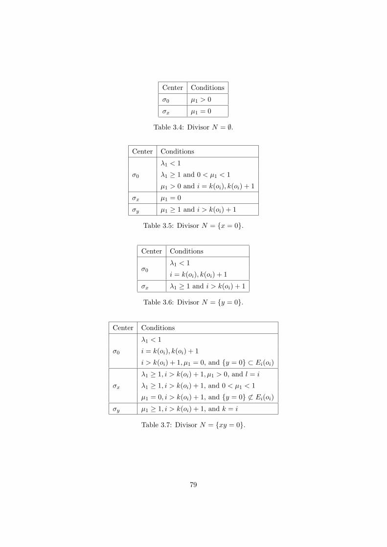
Center Conditions
σ0 µ1 > 0
σx µ1 = 0
Table 3.4: Divisor N = ∅.
Center Conditions
σ0
λ1 < 1
λ1 ≥ 1 and 0 < µ1 < 1
µ1 > 0 and i = k(oi), k(oi) + 1
σx µ1 = 0
σy µ1 ≥ 1 and i > k(oi) + 1
Table 3.5: Divisor N = x = 0.
Center Conditions
σ0
λ1 < 1
i = k(oi), k(oi) + 1
σx λ1 ≥ 1 and i > k(oi) + 1
Table 3.6: Divisor N = y = 0.
Center Conditions
σ0
λ1 < 1
i = k(oi), k(oi) + 1
i > k(oi) + 1, µ1 = 0, and y = 0 ⊂ Ei(oi)
σx
λ1 ≥ 1, i > k(oi) + 1, µ1 > 0, and l = i
λ1 ≥ 1, i > k(oi) + 1, and 0 < µ1 < 1
µ1 = 0, i > k(oi) + 1, and y = 0 6⊂ Ei(oi)
σy µ1 ≥ 1, i > k(oi) + 1, and k = i
Table 3.7: Divisor N = xy = 0.
79
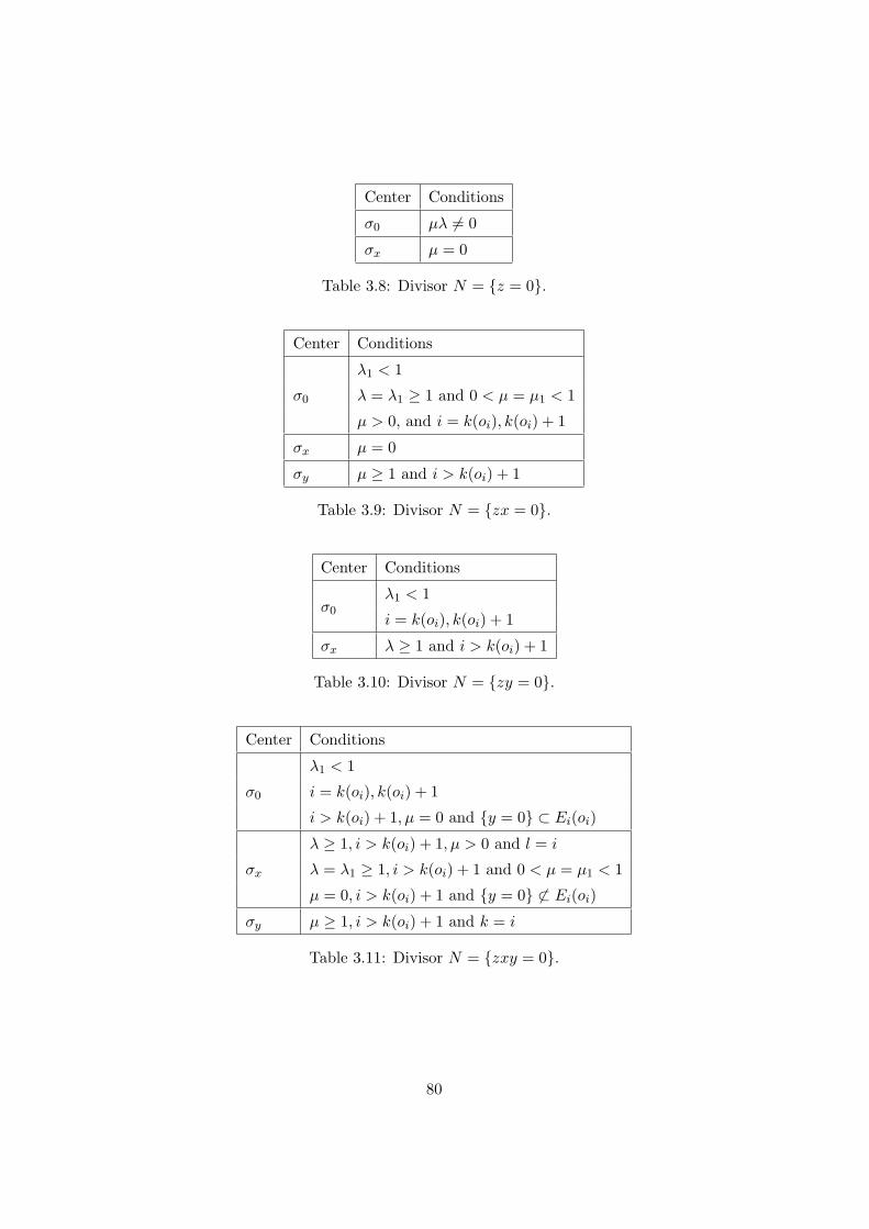
Center Conditions
σ0 µλ 6= 0
σx µ = 0
Table 3.8: Divisor N = z = 0.
Center Conditions
σ0
λ1 < 1
λ = λ1 ≥ 1 and 0 < µ = µ1 < 1
µ > 0, and i = k(oi), k(oi) + 1
σx µ = 0
σy µ ≥ 1 and i > k(oi) + 1
Table 3.9: Divisor N = zx = 0.
Center Conditions
σ0
λ1 < 1
i = k(oi), k(oi) + 1
σx λ ≥ 1 and i > k(oi) + 1
Table 3.10: Divisor N = zy = 0.
Center Conditions
σ0
λ1 < 1
i = k(oi), k(oi) + 1
i > k(oi) + 1, µ = 0 and y = 0 ⊂ Ei(oi)
σx
λ ≥ 1, i > k(oi) + 1, µ > 0 and l = i
λ = λ1 ≥ 1, i > k(oi) + 1 and 0 < µ = µ1 < 1
µ = 0, i > k(oi) + 1 and y = 0 6⊂ Ei(oi)
σy µ ≥ 1, i > k(oi) + 1 and k = i
Table 3.11: Divisor N = zxy = 0.
80

Theorem 3.8.2. Let N be a normal crossings divisor of a germ of a complex
manifold (M,o) of dimension 3. Let S be the germ of a quasi-ordinary
surface at o with trivial limit of tangents. Set Γ = P∗S〈M/N〉. Let L be one
of the admissible centers for S considered in table (3.3). Set Λ = P∗L〈M/N〉.Let Γ be the proper inverse image of Γ by the blow up of P∗〈M/N〉 with
center Λ. Then
Γ ⊂ Ω and Γ = P∗eS〈M/N〉.
Proof. Let λ be the only limit of tangents of S at o. By Lemma 3.5.2 it is
enough to prove that
CΛ(Γ) ∩ σ−1(L) ⊂ Λ. (3.8.1)
holds in order to prove that Γ ⊂ Ω.
(i) Set θ = ξdx+ ηdy + ζdz = ζ(dz − pdx− qdy).(v1) Set L = x = y = z = 0. Hence Λ = x = y = z = 0. We identify L
with the zero section x = y = z = 0 of PLM . We identify Λ with the zero
section x = y = z = 0 of PΛP∗〈M/N〉. Near λ,
σ : PΛP∗〈M/N〉 → PLM
is given by
σ(x, y, z, p, q) = (x, y, z).
Hence, σ−1(L) = Λ.
(v2) Set L = x = z = 0. Hence Λ = x = z = q = 0 and σ(x, y, z, p, q) =
(x, y, z). Since µ1 = 0,
λ2 ≥ λ1 ≥ 1. (3.8.2)
Since
z = aλ10xλ1 + . . .+ aλ2µ2x
λ2yλ2 + · · ·
there is a unit ε of Cx1m , y
1m such that
q =∂z
∂y= xλ2yµ2−1ε (3.8.3)
for some integer m. It follows from (3.8.2) and (3.8.3) that Γ is contained
in a hypersurface
qn +n−1∑i=0
aiqi = 0
81

where ai ∈ Cx, y and ai ∈ (x)n−i. Hence there are ai ∈ (x) such that
CΛ(Γ) is contained in an hypersurface
qn +n−1∑i=0
aiqi = 0
and (3.8.1) holds.
(ii) Set N = x = 0, hence
θ = ξdx
x+ ηdy + ζdz = ζ(dz − pdx
x− qdy).
(x1) Assume that µ1 ≥ 1. If L = x = y = z = 0, Λ = x = y = z = p = 0and σ(x, y, z, p, q) = (x, y, z).
Since there is a unit ε such that z = xλ1yµ1ε, there is a unit δ such that
p = xλ1yµ1δ. Since λ1 + µ1 > 2,
CΛ(Γ) ⊂ p = 0.
Hence, (3.8.1) holds.
Assume L = y = z = 0. Hence Λ = y = z = p = 0. If µ1 > 1, the
argument is similar to the previous one. Assume µ1 = 1.
There are units ε1, ε2 of Cx1m , y
1m such that
z = xλ1yε1, p = xλ1yε2.
Hence CΛ(Γ) ∩ σ−1(L) ⊂ p = 0.(x2) Since L = x = z = 0, Λ = x = z = p = q = 0. There are units ε of
Cx1m , y
1m , ε1, . . . , ε4 of Cx
1m , y
1m such that
z = xλ1ε1 = xλ1ε+ xλ2yµ2ε2, p = xλ1ε3, q = xλ2yµ2−1ε4.
Since µ1 = 0, λ1 > 1. Therefore CΛ(Γ) ⊂ p = 0.Since λ2 ≥ λ1 > 1, µ2 ≥ 1. Therefore CΛ(Γ) ⊂ q = 0.(iii) This case is similar to the previous one.
(iv) If N = xy = 0,
θ = ξdx
x+ η
dy
y+ ζdz = ζ(dz − pdx
x− q dy
y).
Set L = x = y = z = 0. Hence Λ = x = y = z = p = q = 0.
82

There are units εi of Cx1m , y
1m , 1 ≤ i ≤ 3, such that
z = xλ1yµ1ε1, p = zλ1yµ1ε2, q = xλ1yµ1ε3
defines a parametrization of Γreg. Hence there are units ε4, ε5 of Cx1m , y
1m
such that
z = xλ1yµ1ε1, p = zε4, q = zε5
define a parametrization of Γreg. Therefore Γ is contained in the hypersur-
faces with parametrizations given by p = zε4, q = zε5. Hence Γ is contained
in hypersurfaces of the type
pk +k−1∑i=0
aipi = 0, ql +
l−1∑i=0
biqi = 0,
where ai ∈ (zk−i), bi ∈ (zl−i).
Assume that µ1 = 0, L = x = z = 0 or µ1 ≥ 1, L = y = z = 0. In both
cases CΛ(Γ) ⊂ p = q = 0 by the standard arguments.
(v) If N = z = 0,
θ = ξdx+ ηdy + ζdz
z= ζ
(dz
z− pdx− qdy
)= ξ
(dx− rdy − sdz
z
).
(z1) Assume that µ = 0, b ≥ 1 and L = x = z = 0. Hence Λ = x = z =
r = s = 0. There are units ε1, ε2 of Cx1m , ε1, . . . , ε8 of Cx
1m , y
1m such
that
z = xλε1 + xaybε3 = xλε4 (3.8.4)
p =xλ−1
zε2 =
ε5x
=1xε6
(3.8.5)
q =xayb−1
zε7 = xa−λyb−1ε8. (3.8.6)
Hence xε6ξ + ζ = 0, η + xa−λyb−1ε8ζ = 0.
Therefore Γ is contained in the hypersurfaces with parametrizations given
by
s = ε6x, r + xa−λyb−1ε8s = 0.
Hence CΛ(Γ) ∩ x = z = 0 ⊂ r = s = 0.(vi) If N = xz = 0,
θ = ξdx
x+ ηdy + ζ
dz
z= η(dy − rdx
x− sdz
z).
83

Assume that µ 6= 0. Set L = x = y = z = 0. Hence Λ = x = y = z =
r = s = 0. Notice that
z = xλyµε1, p =xλyµ
zε2 = ε3, q =
xλyµ−1
zε4 =
1ε5y
.
ξ + ε3ζ = 0, yε5η + ζ = 0.
u = ε3s = 0, s = yε5.
Hence CΛ(Γ) ∩ ρ−1(L) ⊂ (r = s = 0).
If µ 6= 0 and L = y = z = 0, then Λ = y = z = r = s = 0, and this case
is solved in a similar fashion.
Assume that µ = 0. In this case L = Λ = x = z = 0. This situation is
solved by theorem 3.6.1.
(vii) Set N = yz = 0.If µ 6= 0, we are in the situation of (xz1).
Assume that µ = 0. Set θ = ξdx+ η dyy + ζ dz
z = ξ(dx− r dyy − s
dzz ).
Following the scheme of the previous cases,
z = xλε1 = xλε2 + xaybε3, where∂ε2∂y
= 0
p =xλ−1
zε4 =
1xε5
, q =xayb
zε6 = xa−λybε7,
xε5ξ + ζ = 0, η + aa−λybε7ζ = 0,
s = xε5, r + xa−λybε7s = 0. (3.8.7)
It follows from 3.8.7 that CΛ(Γ) ∩ ρ−1(L) ⊂ r = s = 0 if L = x = y =
z = 0 or L = x = z = 0.
Example 3.8.3. Given δ ∈ Cx1m , ε ∈ Cx
1m , y
1m , λ > 1 and 0 < b < 1,
the surface S with parametrization
z = xλδ + xλybε
verifies the condition (xz3) of Theorem 3.8.1. Hence its logarithmic limits
of tangents relatively to the divisor xz = 0 is trivial. The proper inverse
84

image of S by the blow up with center x = z = 0 admits the parametriza-
tionzx = xλ−1δ1 + xλ+b−1ybε1.
By theorem 3.8.1, the logarithmic limit of tangents of S relatively to the
divisor x zx = 0 is not trivial.
Example (3.8.3) shows that the triviality of limits of tangents is not heredi-
tary by blowing up. Lemma 3.8.4 solves this problem.
Lemma 3.8.4. Let N be the normal crossings divisor of a germ of complex
manifold (M,o) of dimension three. Let S be a surface of M such that the
logarithmic limit of tangents of S along N is trivial. Let π : M → M be
the blow up of M along an admissible center for S and N . Let E be the
exceptional divisor of π. Let p ∈ S ∩ E. If S,N do not verify condition
(xz3) of table (3.3) at o
(i) S has trivial logarithmic limit of tangents along N at p.
(ii) S, N do not verify condition (xz3) at p.
Proof. We will denote by εi a unit of Cx1m , y
1m and by δi a unit of Cx
1m ,
for a convenient m. We will denote by (xy), (yz), (xyz) the situations (xyi),
(yzi), (xyzi) for each i.
(v1) We can assume that z = xλ1yµ1ε1. On the chart (x, yx ,
zx),
zx = xλ1+µ1−1 y
xµ1ε2.
Since λ1 ≥ µ1 ≥ 1 and (λ1, λ2) 6∈ Z2, we are in situation (x1) at each point
of N = x = 0. The same happens in the chart (xy , y,
zy ).
(v2) We can assume that z = xλ1δ1 + xλ2yµ2ε1. On the chart (x, y, zx),
N = x = 0 andzx = xλ1−1δ2 + xλ2−1yµ2ε2.
If λ1 > 2 we are in situation (x2). Assume λ1 < 2. By table (3.2), S admits
the parametrization
x = ( zx)
λ1λ1−1 + ( z
x)λ2
λ1−1 yµ2ε4.
Hence we are in situation (z1).
The cases (x1),(x2),(y1) are similar to the previous cases.
85

(xy1) Assume that λ1 + µ1 ≥ 1. In the chart (x, yx ,
zx), N = x y
x = 0 and
S admits the parametrization
zx = xλ1+µ1−1 y
xµ1ε2.
Let o be a point of N where x 6= 0. If µ1 = 0, S is smooth at o. Otherwise
yx = ( z
x)1
µ1 ε3.
Hence we are in situation (z1). The same holds at a point of N where yx 6= 0.
The situation is similar in the chart (xy , y,
zy ).
Assume that λ1 + µ1 < 1. In the chart (xz ,
yz , z), N = x
zyz z = 0 and S
admits the parametrization
z = (xz )
λ11−λ1−µ1 (y
z )µ1
1−λ1−µ1 ε2.
We are in the situation (xyz) at (0, 0, 0). Let o be a point of N where xz 6= 0.
If µ1 = 0 or 2λ1 + µ1 = 1, S is smooth at o. If µ1 6= 0 and 2λ1 + µ1 6= 1, we
are in situation (x2) or in situation (z1). The situation is similar at a point
of N where yz 6= 0.
The cases (xy2) and (xy3) are quite similar.
(z1) The blow up produces situation (z1) if λ ≥ 2 and (x1) if λ < 2.
(xz1) Assume that we blow up σ0. Assume that λ + µ ≥ 1. In the chart
(x, yx ,
zx), N = x z
x = 0 and S admits the parametrization
zx = xλ+µ−1 y
xµε2.
Assume that λ + µ > 1. We are in situation (xz1) at (0, 0, 0). Let o be a
point of N . If x 6= 0, S is in situation (yz) at o.
Assume that λ + µ = 1. Setting x = zx , y = x, z = y
x , S admits the
parametrization
z = x1µ ε4 and N = xy = 0.
We are in situation (xy) at (0, 0, 0). Let o be a point of N . If y 6= 0 we are
in situation (x2) at o.
The case λ+ µ < 1 is similar to the case λ+ µ > 1.
(xz2) We can assume that z = xλδ1 + xaybε1. On the chart (x, y zx), N =
x zx = 0 and
zx = xλ−1δ2 + xa−1ybε2.
86
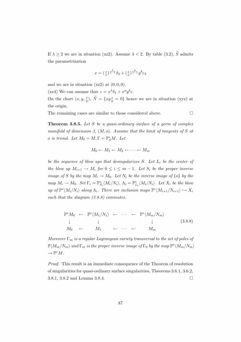
If λ ≥ 2 we are in situation (xz2). Assume λ < 2. By table (3.2), S admits
the parametrization
x = ( zx)
λλ−1 δ3 + ( z
x)a
λ−1 ybε3
and we are in situation (xz2) at (0, 0, 0).
(xz4) We can assume that z = xλδ1 + xaybε.
On the chart (x, y, zy ), N = xy z
y = 0 hence we are in situation (xyz) at
the origin.
The remaining cases are similar to those considered above.
Theorem 3.8.5. Let S be a quasi-ordinary surface of a germ of complex
manifold of dimension 3, (M,o). Assume that the limit of tangents of S at
o is trivial. Let M0 = M,Γ = P∗SM . Let
M0 ←M1 ←M2 ← · · · ←Mm
be the sequence of blow ups that desingularizes S. Let Li be the center of
the blow up Mi+1 → Mi for 0 ≤ i ≤ m − 1. Let Si be the proper inverse
image of S by the map Mi →M0. Let Ni be the inverse image of o by the
map Mi →M0. Set Γi = P∗Si〈Mi/Ni〉, Λi = P∗Li
〈Mi/Ni〉. Let Xi be the blow
up of P∗〈Mi/Ni〉 along Λi. There are inclusion maps P∗〈Mi+1/Ni+1〉 → Xi
such that the diagram (3.8.8) commutes.
P∗M0 ← P∗〈M1/N1〉 ← · · · ← P∗〈Mm/Nm〉↓ ↓ ↓M0 ← M1 ← · · · ← Mm
(3.8.8)
Moreover Γm is a regular Lagrangean variety transversal to the set of poles of
P〈Mm/Nm〉 and Γm is the proper inverse image of Γ0 by the map P∗〈Mm/Nm〉→ P∗M .
Proof. This result is an immediate consequence of the Theorem of resolution
of singularities for quasi-ordinary surface singularities, Theorems 3.6.1, 3.6.2,
3.8.1, 3.8.2 and Lemma 3.8.4.
87

Bibliography
[1] A. Araujo, O. Neto, Moduli of Germs of Legendrian Curves , Ann.
Fac. Sci. Toulouse Math., Vol. XVIII, 4, 2009, 645-657.
[2] C. Ban, Aureole of a quasi-ordinary singularity, Proc. Amer. Math.
Soc., 120 (1994), 393-404.
[3] E. Bierstone and P. Milman, A simple constructive proof of canoni-
cal resolution of singularities.Effective methods in algebraic geometry
(Castiglioncello, 1990), Progr. Math. 94, Birkhauser, Boston, MA,
(1991), 11-30
[4] C. Ban and L. Mcewan, Canonical resolution of a quasi-ordinary sur-
face singularity , Canadian Journal of Mathematics , Vol. 52(6) (2000),
1149-1163.
[5] E. Brieskorn and H. Knorrer, Plane Algebraic Curves, Birkhauser
(1986).
[6] J. Cabral, O. Neto, Microlocal versal deformations of the plane curves
yk = xn, C.R. Acad Sci. Paris 340 (2005), no. 2, 141-146.
[7] C. Delorme, Sur les modules des singularites des courbes planes, Bull.
Soc. Math. France, 106, (1978) 417-446.
[8] G.-M. Greuel and G. Pfister, Moduli for singularities, J.-P. Brasselet
(ed.), Singularities, Lond. Math. Soc. Lect. Note Ser., 201, (1994)
119-146.
[9] H. Hironaka, Resolution of singularities of an algebraic variety over a
field of characteristic zero: I, II , Ann. of Math. (2) 79 (1964), 109-326.
88

[10] M. Kashiwara and T. Kawai, On holonomic systems of microdifferen-
tial equations. III: Systems with regular singularities. Publ. Res. Inst.
Math. Sci. 17, (1981) 813-979.
[11] M. Kashiwara, Systems of microdifferential equations, Progress in
Mathematics, 34. Birkhauser.
[12] M. Kashiwara, Schapira, P., Sheaves on Manifolds, (Grundlehren Der
Mathematischen Wissenschaften), Springer Verlag (2002).
[13] D.T. Le and B. Teissier, Limites d’espaces tangentes en geometrie
analitique, Comment. Math. Helv., 63, (1988), 540-578.
[14] J. Lipman, Quasi-ordinary singularities of embedded surfaces, Ph.D.
thesis, Harvard University, 1965.
[15] J. Lipman, Topological invariants of quasi-ordinary singularities,
Mem. Amer. Math. Soc., No. 74, Amer. Math. Soc., Providence, RI,
1988, 1-107.
[16] O. Neto, A microlocal Riemann-Hilbert correspondence., Compositio.
Math., 127, (2001), No. 3, 229-241.
[17] O. Neto, Equisingularity and Legendrian curves, Bull. London Math.
Soc. 33 (2001), 527-534.
[18] O. Neto, Blow up for a holonomic system.Publ. Res. Inst. Math. Sci.
29 (1993), no. 2, 167-233.
[19] O. Neto, Systems of meromorphic microdifferential equations. Singu-
larities and differential equations (Warsaw, 1993), 259-275, Banach
Center Publ., 33, Polish Acad. Sci., Warsaw, 1996.
[20] R. Peraire, Moduli of plane curve singularities with a single character-
istic exponent, Proc. Am. Math. Soc. 126, No.1, (1998), 25-34.
[21] F. Pham, Singularites des Systemes Differentiels de Gauss-Manin,
(Progress in Mathematics), Birkhauser (1979).
89

[22] O. Villamayor, Constructiveness of Hironaka’s resolution. Ann. Sci.
Ecole Norm. Sup. (4) 22 (1989), no. 1, 1-32.
[23] O. Zariski , Le probleme des modules pour les branches planes, Her-
mann (1970).
90