Tidewater glaciers of Svalbard: Recent changes and ...polish.polar.pan.pl/ppr30/PPR30-085.pdf ·...
58
Tidewater glaciers of Svalbard: Recent changes and estimates of calving fluxes Małgorzata BŁASZCZYK 1,2 , Jacek A. JANIA 1 and Jon Ove HAGEN 3 1 Wydział Nauk o Ziemi, Uniwersytet Śląski, Będzińska 60, 41−200 Sosnowiec, Poland <[email protected]> <[email protected]> 2 Instytut Geofizyki PAN, Księcia Janusza 64, 01−452 Warszawa, Poland 3 Department of Geosciences, University of Oslo, POBox 1047 Blindern, N−0316 Oslo, Norway <[email protected]> Abstract: The purpose of this study is to describe the current state of tidewater glaciers in Svalbard as an extension of the inventory of Hagen et al. (1993). The ice masses of Svalbard cover an area of ca 36 600 km 2 and more than 60% of the glaciated areas are glaciers which terminate in the sea at calving ice−cliffs. Recent data on the geometry of glacier tongues, their flow velocities and front position changes have been extracted from ASTER images acquired from 2000–2006 using automated methods of satellite image analysis. Analyses have shown that 163 Svalbard glaciers are of tidewater type (having contact with the ocean) and the total length of their calving ice−cliffs is 860 km. When compared with the previous inventory, 14 glaciers retreated from the ocean to the land over a 30–40 year period. Eleven formerly land−based glaciers now terminate in the sea. A new method of assessing the dy− namic state of glaciers, based on patterns of frontal crevassing, has been developed. Tide− water glacier termini are divided into four groups on the basis of differences in crevasse pat− terns and flow velocity: (1) very slow or stagnant glaciers, (2) slow−flowing glaciers, (3) fast−flowing glaciers, (4) surging glaciers (in the active phase) and fast ice streams. This classification has enabled us to estimate total calving flux from Svalbard glaciers with an accuracy appreciably higher than that of previous attempts. Mass loss due to calving from the whole archipelago (excluding Kvitøya) is estimated to be 5.0–8.4 km 3 yr −1 (water equiv− alent – w.e.), with a mean value 6.75 ± 1.7 km 3 yr −1 (w.e.). Thus, ablation due to calving con− tributes as much as 17–25% (with a mean value 21%) to the overall mass loss from Svalbard glaciers. By implication, the contribution of Svalbard iceberg flux to sea−level rise amounts to ca 0.02 mm yr −1 . Also calving flux in the Arctic has been considered and the highest an− nual specific mass balance attributable to iceberg calving has been found for Svalbard. Key words: Arctic, Svalbard, tidewater glaciers, calving flux, ASTER. Introduction Climate warming is more pronounced in the Arctic than in the mid−latitudes (cf. ACIA 2005, IPCC 2007). The response of glaciers to climate change is a good mea− Pol. Polar Res. 30 (2): 85–142, 2009 vol. 30, no. 2, pp. 85–142, 2009
Transcript of Tidewater glaciers of Svalbard: Recent changes and ...polish.polar.pan.pl/ppr30/PPR30-085.pdf ·...

Tidewater glaciers of Svalbard:Recent changes and estimates of calving fluxes
Małgorzata BŁASZCZYK1,2, Jacek A. JANIA1 and Jon Ove HAGEN3
1 Wydział Nauk o Ziemi, Uniwersytet Śląski, Będzińska 60, 41−200 Sosnowiec, Poland<[email protected]> <[email protected]>
2 Instytut Geofizyki PAN, Księcia Janusza 64, 01−452 Warszawa, Poland3 Department of Geosciences, University of Oslo, POBox 1047 Blindern, N−0316 Oslo, Norway
Abstract: The purpose of this study is to describe the current state of tidewater glaciers inSvalbard as an extension of the inventory of Hagen et al. (1993). The ice masses of Svalbardcover an area of ca 36 600 km2 and more than 60% of the glaciated areas are glaciers whichterminate in the sea at calving ice−cliffs. Recent data on the geometry of glacier tongues,their flow velocities and front position changes have been extracted from ASTER imagesacquired from 2000–2006 using automated methods of satellite image analysis. Analyseshave shown that 163 Svalbard glaciers are of tidewater type (having contact with the ocean)and the total length of their calving ice−cliffs is 860 km. When compared with the previousinventory, 14 glaciers retreated from the ocean to the land over a 30–40 year period. Elevenformerly land−based glaciers now terminate in the sea. A new method of assessing the dy−namic state of glaciers, based on patterns of frontal crevassing, has been developed. Tide−water glacier termini are divided into four groups on the basis of differences in crevasse pat−terns and flow velocity: (1) very slow or stagnant glaciers, (2) slow−flowing glaciers, (3)fast−flowing glaciers, (4) surging glaciers (in the active phase) and fast ice streams. Thisclassification has enabled us to estimate total calving flux from Svalbard glaciers with anaccuracy appreciably higher than that of previous attempts. Mass loss due to calving fromthe whole archipelago (excluding Kvitøya) is estimated to be 5.0–8.4 km3 yr−1 (water equiv−alent – w.e.), with a mean value 6.75 ± 1.7 km3 yr−1 (w.e.). Thus, ablation due to calving con−tributes as much as 17–25% (with a mean value 21%) to the overall mass loss from Svalbardglaciers. By implication, the contribution of Svalbard iceberg flux to sea−level rise amountsto ca 0.02 mm yr−1. Also calving flux in the Arctic has been considered and the highest an−nual specific mass balance attributable to iceberg calving has been found for Svalbard.
Key words: Arctic, Svalbard, tidewater glaciers, calving flux, ASTER.
Introduction
Climate warming is more pronounced in the Arctic than in the mid−latitudes (cf.ACIA 2005, IPCC 2007). The response of glaciers to climate change is a good mea−
Pol. Polar Res. 30 (2): 85–142, 2009
vol. 30, no. 2, pp. 85–142, 2009

sure of long−term climate trends and the environmental consequences of warming.There is much evidence that Svalbard glaciers are very sensitive to climatic change,presumably because the influence of the North Atlantic ocean current system(Walczowski and Piechura 2006). The ice masses of Svalbard cover an area of ca 36600 km2 and are among the largest glaciated areas in the Arctic (Hagen et al. 1993;Dowdeswell and Hambrey 2002). Glaciers that flow into the sea and terminate in anice cliff from which icebergs are discharged are called tidewater glaciers (Van derVeen 1996) and the breakage of icebergs from the cliff is termed “calving”. The termcalving glaciers is also used; these are defined as glaciers calving brash and icebergsinto lakes, fiords or open sea (Post and Motyka 1995). Tidewater glaciers are a char−acteristic feature of the Svalbard environment. They constitute more than 60% of thetotal ice−covered area. A recent study by Dowdeswell et al. (2008) indicates thatcalving from the Austfonna ice cap (8120 km2) on Nordaustlandet, NE Svalbardalone amounts to 2.5 km3 yr−1. This represents as much as 30–40% of the annual ab−lation from this ice cap. This is a general indication of the importance of tidewaterglaciers for the mass budget of Svalbard ice masses.
Climate warming affects tidewater glaciers through changes in the surfacemass balance components, the dynamic response of glaciers, and the influence ofwarmer water on the ice cliff – ocean water interface. Generally, without takinginto account active surges of glaciers discussed later in this paper, increased pro−duction of icebergs is a result of the dynamic response of glaciers terminating inthe ocean to a warmer environment. Such a process has been evident in Greenlandover the last few years (e.g. Dowdeswell 2006; Rignot and Kanagaratnam 2006;Nettles et al. 2008). The greater the transfer of glacier ice from land to the sea, thegreater the eustatic sea level rise. We consider that this effect was underestimatedby the last IPCC Report (IPCC 2007).
Svalbard glaciers contribute to global sea level rise because of their negativemass balance. Mass loss due to calving is still not properly studied. Existing esti−mates of the volume of icebergs lost by calving are both rather crude (Dowdeswell1989; Lefauconnier and Hagen 1991; Hagen et al. 2003a; Dowdeswell and Hagen2004) and variable, presumably due to the limited availability of data. To better es−timate the mass of ice calved by tidewater glaciers in Svalbard, more data about theglaciers themselves and processes responsible for calving are needed.
A detailed glacier inventory of the Svalbard archipelago was compiled byHagen et al. (1993) in the “Glacier Atlas of Svalbard and Jan Mayen”. But almostall of the data presented there were derived from topographic maps at a scale of1:100 000 (prepared from aerial photos taken in 1936) and more recent aerial pho−tographs taken before 1990. As a result of the retreat and thinning of tidewater gla−ciers in Svalbard observed since the beginning of the 20th century (e.g. Koryakin1975; Jania 1988a, 2002; Hagen et al. 1993, 2005) this inventory needs to be up−dated. The aim of this paper is to document the current status of tidewater glaciersin Svalbard, especially in terms of the nature of their calving fronts and present dy−
86 Małgorzata Błaszczyk, Jacek A. Jania and Jon Ove Hagen

namic state. The paper aims to continue the work of Hagen et al. (1993) focusingonly on the tidewater glaciers. Glaciers draining into lakes with no contact with thesea are not considered.
Recent data on the geometry of glacier tongues, their flow velocities and frontposition changes have been extracted from satellite imagery. Characteristics of alltidewater glaciers of Svalbard were examined (see Appendix) and compared withdata presented by Hagen et al. (1993). A more precise estimate of ice mass loss bycalving from the whole archipelago is another objective of this work. The calcula−tion of ice fluxes is based upon observations of calving glaciers on satellite imagesand very sparse ground survey data (published and unpublished). The main sourcesof data used are ASTER images acquired from 2000–2006, mainly in July and Au−gust (cf. Table 1). The relatively long intervals between acquisition dates for manyASTER image pairs are due to the infrequent breaks in the cloud cover in the abla−tion season.
Tidewater glaciers of Svalbard 87
Table 1ASTER and Landsat 7 imagery (granules) used in this studies; No. – number of the scene as
presented on Fig. 2; D – acquisition date: dd−mm−yyyy.
No. Data Granule ID D No. Data Granule ID D
ASTER ASTER
1 AST_L1A.003:2007905507 24.07.2002 23 AST_L1A.003:2025232924 7.08.2004
2 AST_L1A.003:2003624865 25.07.2001 24 AST_L1A.003:2036235228 15.08.2006
3 AST_L1A.003:2007910399 25.07.2002 25 AST_L1A.003:2030183765 23.07.2005
4 AST_L1A.003:2008754102 23.07.2002 26 AST_L1A.003:2035266221 20.07.2006
5 AST_L1A.003:2007905506 24.07.2002 27 AST_L1A.003:2029911899 6.07.2005
6 AST_L1A.003:2015776657 5.08.2003 28 AST_L1A.003:2007780347 11.07.2002
7 AST_L1A.003:2015776686 5.08.2003 29 AST_L1A.003:2003775114 5.08.2001
8 AST_L1A.003:2025232928 7.08.2004 30 AST_L1A.003:2030201287 24.07.2005
9 AST_L1A.003:2025232921 7.08.2004 31 AST_L1A.003:2008563292 5.07.2002
10 AST_L1A.003:2030183769 23.07.2005 32 AST_L1A.003:2007780343 11.07.2002
11 AST_L1A.003:2025232939 7.08.2004 33 AST_L1A.003:2007780342 11.07.2002
12 AST_L1A.003:2009046994 17.08.2000 34 AST_L1A.003:2007780344 11.07.2002
13 AST_L1A.003:2009046998 17.08.2000 35 AST_L1A.003:2007714526 12.07.2002
14 AST_L1A.003:2015312591 13.07.2003 36 AST_L1A.003:2003304043 16.06.2001
15 AST_L1A.003:2035244797 19.07.2006 37 AST_L1A.003:2003304045 16.06.2001
16 AST_L1A.003:2030183768 23.07.2005 38 AST_L1A.003:2030171638 18.07.2005
17 AST_L1A.003:2030183770 23.07.2005 39 AST_L1A.003:2030171637 18.07.2005
18 AST_L1A.003:2035364191 23.07.2006 40 AST_L1A.003:2003775127 5.08.2001
19 AST_L1A.003:2025153126 25.07.2004 LANDSAT 7
20 AST_L1A.003:2025153125 25.07.2004 41 l71211004_00419990709 09.07.1999
21 AST_L1A.003:2025153146 25.07.2004 42 l71215002_00220010710 10.07.2001
22 AST_L1A.003:2016494057 27.07.2003 43 l72218003_00319990710 10.07.1999

The Svalbard glaciers
The Svalbard archipelago is located at the NW limit of the European continen−tal shelf between 76.50–80.80�N and 10–34�E. It consists of four main islands:Spitsbergen, Nordaustlandet, Barentsøya, Edgeøya (Fig. 1) and ca 150 smaller is−lands. The total area of Svalbard is 62 800 km2 and ca 60%, or about 36 600 km2 ofthis area is covered by glaciers (Hagen et al. 1993). Various types of glacier arefound. Dominant by area are the large continuous ice masses that are divided intoindividual ice streams by mountain ridges and nunataks. Small cirque glaciers arealso numerous, especially in the alpine regions of western Spitsbergen. Severallarge ice caps are located in the relatively flat areas of eastern Svalbard. These icecaps calve into the sea. The total length of calving ice fronts in Svalbard is about1000 km. All margins are grounded (Dowdeswell 1989). Maximum ice thick−nesses of 500–600 m occur in Amundsenisen in South Spitsbergen and theAustfonna ice cap in Nordaustlandet. The total ice volume of Svalbard is estimatedto be ca 7 000 km3 (Hagen et al. 1993).
Permafrost conditions prevail in Svalbard and the depth of permafrost variesfrom 50 to several hundred meters. However, the glaciers in Svalbard are oftenpolythermal, which means that some parts of the ice masses are temperate (at thepressure melting point) while other parts are at sub−freezing temperatures. In generalthe lower and thinner parts of the glaciers are frozen, to a depth of as much as 100 m.The consequence of this is that the thinner glaciers are often frozen to the ground.The thicker glaciers have temperate parts from which water drains throughout theyear. Large icings are often formed in front of land−terminating polythermal glacierswhen meltwater slowly drains out of the glacier during winter and freezes on thecold frozen ground. Winter drainage can often be observed in front of tidewater gla−ciers as an upwelling of water at the calving front.
Owing to the low ice temperatures and fairly low accumulation rates, the flowrate of Svalbard glaciers is generally low. In general, glaciers that terminate onland flow much more slowly than tidewater glaciers. Typical surface velocities areless than 10 m yr−1 close to the equilibrium line altitude of glaciers that terminateon land, whereas some calving glaciers have much higher velocities – 100 m yr−1 ormore. Kronebreen in Kongsfjorden is by far the fastest flowing glacier in Svalbard,having a velocity of about 2 m d−1, or 700–800 m yr−1 at the calving front.
Surging glaciers are common in Svalbard (Liestøl 1969; Jania 1988a; Lefau−connier and Hagen 1991; Hagen et al. 1993; Dowdeswell et al. 1991; Jiskoot et al.2000). A surge event results in a large ice flux from the higher to the lower regionsof a glacier, usually accompanied by a rapid advance of the glacier front and, in thecase of tidewater glaciers, by increased iceberg production. For instance, the 1250km2 Hinlopenbreen, which surged in 1970, calved about 2 km3 of icebergs in a sin−gle year (Liestøl 1973).
88 Małgorzata Błaszczyk, Jacek A. Jania and Jon Ove Hagen

Tidewater glaciers of Svalbard 89
Fig. 1. Location map of Svalbard and glaciated area of the archipelago as visible on mosaic of ASTERand Landsat 7 images used in this study (cf. Table 1 and Fig. 2).

90 Małgorzata Błaszczyk, Jacek A. Jania and Jon Ove Hagen
Fig. 2. Sketch of coverage of Svalbard by ASTER (solid frame) and Landsat 7 (dashed frame) imag−ery used in this inventory (Nos. of scenes correspond to Nos. in Table 1).

Observations of front positions indicate a general retreat of glaciers in Sval−bard over the last 80 years. The Little Ice Age ended in Svalbard about 100 yearsago, when most glaciers reached their maximum Holocene extent.
Annual mass−balance measurements have been made on several (<1%) Sval−bard glaciers for up to 40 years. Consistent with the general recession, most ofthese glaciers have a negative mass balance, but with no discernible change intrend. The winter accumulation undergoes an inter−annual variations but they arefairly small. The mean summer ablation is also stable with no obvious trend. How−ever, there are large inter−annual variations in the annual net mass balance and thesummer ablation clearly controls these variations. While low−altitude glaciers areshrinking steadily, glaciers with high−altitude accumulation areas have mass bal−ances closer to zero or even positive in some years.
Estimates of the total mass balance of Svalbard glaciers vary between −5 to −14km3 yr−1 or a specific net mass balance of −0.12 to −0.38 m yr−1, equivalent to a sealevel rise of 0.01 to 0.04 mm yr−1 (Hagen et al. 2003a, b). There are thus still largeuncertainties about the overall mass balance and the calving flux. In this paper wewill attempt to improve the latter estimate.
Methods
The optical sensor ASTER (Advanced Spaceborne Thermal Emission and Re−flection Radiometer) on board the Terra satellite has proved to be a useful tool forglacier mapping and monitoring (e.g. Paul et al. 2002; Paul and Kääb 2005;Svoboda and Paul 2007; Bolch et al. 2008; Molnia 2008; http://www.glims.org/).ASTER imagery has relatively high spatial resolution in the visible and near visi−ble IR bands (15 m and 30 m), and ASTER’s along−track stereo sensor allowsphotogrammetric DEM generation. ASTER images have previously been used forstudies of Svalbard glaciers (e.g. Dowdeswell and Benham 2003; Kääb et al. 2005;Kääb 2005). Owing to a dearth of cloud− and snow−free ASTER images ofSvalbard, however, three Landsat 7 images were also used in this study. The im−ages used are listed in Table 1 and shown on Figs 1 and 2, and were acquired over7 summer ablation seasons.
The most important morphometric features of all tidewater glaciers are: (1)glacier area, (2) length of centerline, (3) glacier mean slope, (4) length of crevassedzone, (5) area of crevassed zone close to the active calving front, and (6) length ofice cliff. These features were measured on the geocoded ASTER and Landsat 7 im−ages using ArcGIS software. The surface velocity fields of glacier termini were de−rived from ASTER image pairs and from published and unpublished ground sur−vey data.
The delineation of glacier basins is crucial for a proper glacier inventory. Theboundaries of the Svalbard tidewater glaciers were mapped automatically (Fig. 3a)
Tidewater glaciers of Svalbard 91
using the ratio of ASTER bands 3 (15 m resolution) and 4 (30 m resolution) to gen−erate a glacier mask, and by automated raster line to vector conversion. A panchro−matic False Colour Composite (FCC) of ASTER bands 432 was used to manuallydelineate those glaciers for which expert knowledge was needed (Fig. 3b).
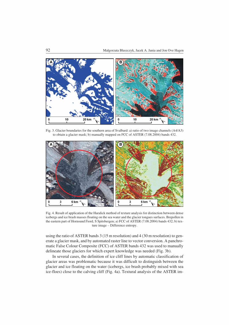
In several cases, the definition of ice cliff lines by automatic classification ofglacier areas was problematic because it was difficult to distinguish between theglacier and ice floating on the water (icebergs, ice brash probably mixed with seaice−floes) close to the calving cliff (Fig. 4a). Textural analysis of the ASTER im−
92 Małgorzata Błaszczyk, Jacek A. Jania and Jon Ove Hagen
Fig. 3. Glacier boundaries for the southern area of Svalbard: a) ratio of two image channels (A4/A3)to obtain a glacier mask; b) manually mapped on FCC of ASTER (7.08.2004) bands 432.
Fig. 4. Result of application of the Haralick method of texture analysis for distinction between denseicebergs and ice brash masses floating on the sea water and the glacier tongues surfaces. Brepollen inthe eastern part of Hornsund Fiord, S Spitsbergen; a) FCC of ASTER (7.08.2004) bands 432; b) tex−
ture image – Difference entropy.

ages (using MaZda software; Haralick et al. 1973; Rudnicki 2002) was used to dis−tinguish the ice floating in the ocean from the glacier body (Fig. 4b).
DEMs prepared from the ASTER stereo bands (in PCI Orthoengine software)were used to delineate boundaries between individual glacier basins. Definition ofglacier boundaries was achieved by visual supervision of the “watershed” proce−dure in the ArcGIS software system and other methods such as slope and aspectanalysis (Fig. 5). In cases where slopes are low, as in the vicinity of ice divides andin ice cap interiors, the delineation of any particular glacier basin is difficult. Thesame is true in respect of glacier tributaries and confluences. In such cases, delin−eation is necessarily subjective (cf. Jania 1988b; Hagen et al. 1993). The length ofthe glacier along its centre−line, the length of the active calving front and the lengthof the terminal ice cliff were derived manually using ArcGIS software. Other spe−cific methods applied in this study are outlined in subsequent paragraphs.
Inventory of tidewater glaciers
The inventory of tidewater glaciers listed in the Appendix contains an identifi−cation number for each glacier, the name of the glacier unit, information on the sat−ellite imagery employed to map the glacier, data on the length and area of the gla−cier, the length and area of the terminal crevassed zone, the length of the terminalice−cliff, the average ice−marginal retreat rate (area of glacier retreat divided by thelength of the ice cliff), the retreat rate measured along the glacier center−line, asymbol for the glacier front type, and an estimate of the calving intensity (Table Iin the Appendix).
Tidewater glaciers of Svalbard 93
Fig. 5. Three dimensional view of glacier basins in SE Spitsbergen, processed from stereoscopic AS−TER images (7.08.2004); vertical scale exaggerated 5x. The boundaries of basins are marked by solid
lines. H – peak of Hornsundtind mountain 1431 m a.s.l.

The system used for the identification of glaciers in this work is the same as thatused in Hagen’s et al. (1993) inventory. It includes the number of regions ofSvalbard (see Appendix: Fig. 12), the glacier identification number from the WorldGlacier Inventory (WGI) and the name of glacier basin. Some glaciers which wereformerly confluent are now separated, owing to significant recession (Fig. 6a, b).Other glaciers that are still confluent have very different dynamics, in which casethey are classified separately for the purpose of our inventory. They still have thecommon WGI identification number (Appendix – Table I), but are given either sepa−rate names derived from topographic maps (see an example on Fig. 6b) or consecu−tive numbers (for instance Vasilievbreen 1, Vasilievbreen 2, cf. Fig. 6c).
94 Małgorzata Błaszczyk, Jacek A. Jania and Jon Ove Hagen
Fig. 6. Left: Hambergbreen (121 04) now separated into two components after retreat: Hamberg−bereen and Sykorabreen; a) front position in 1936, a portion of the topographic map 1:100 000, sheetC12 Markhambreen, courtesy of the NPI; b) ASTER image (7.08.2004); c) Vasilievbreen (121 04)now separated into three components following different dynamics of particular segments (ASTER,
7.08.2004).
The inventory includes data on the area of the glaciers. It must be emphasised,however, that the “area of tidewater glacier” is defined differently from that of its“total basin”. When a tidewater glacier has a compound basin, only that part of itfeeding the calving front was taken into consideration and presented here as the “gla−cier area”. This implies that tributary glaciers clearly separated from the main basinby moraines were not included in the “glacier area” measurements. Similarly, mar−ginal sections of tidewater glaciers that terminate on land were not included in thearea calculation. This reflects the general objective of this paper, which is the assess−ment of the dynamics of tidewater glaciers and the calculation of iceberg fluxes fromthem. As a result, data on the glacier area presented in the atlas of Hagen et al. (1993)are not directly comparable with the values presented in this inventory.
For the large ice caps of Nordaustlandet, the “areas of glacier basins” were takenfrom Hagen et al. (1993). Owing to incomplete ablation season coverage by ASTERscenes, Landsat 7 images were substituted for these areas. A consequence of this wasthat it was not possible to define ice divides and glacier borders by the method de−scribed earlier. The other parameters for that island were updated using the methodsdescribed earlier. Low−resolution ASTER images (150×150 m) available in the LPDAAC inventory (http://edcimswww.cr.usgs.gov/pub/imswelcome/) were used inthe categorization of Kvitøyjøkulen (on the small island Kvitøya, NE Svalbard).
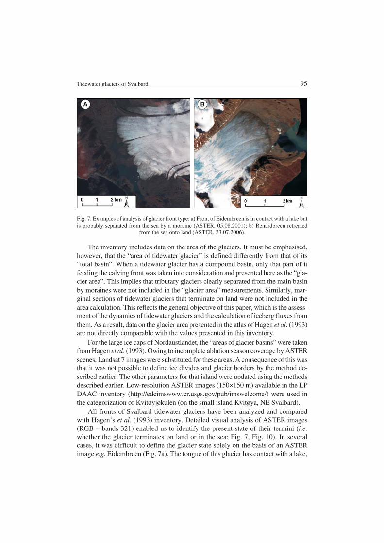
All fronts of Svalbard tidewater glaciers have been analyzed and comparedwith Hagen’s et al. (1993) inventory. Detailed visual analysis of ASTER images(RGB – bands 321) enabled us to identify the present state of their termini (i.e.whether the glacier terminates on land or in the sea; Fig. 7, Fig. 10). In severalcases, it was difficult to define the glacier state solely on the basis of an ASTERimage e.g. Eidembreen (Fig. 7a). The tongue of this glacier has contact with a lake,
Tidewater glaciers of Svalbard 95
Fig. 7. Examples of analysis of glacier front type: a) Front of Eidembreen is in contact with a lake butis probably separated from the sea by a moraine (ASTER, 05.08.2001); b) Renardbreen retreated
from the sea onto land (ASTER, 23.07.2006).

but no canal can be identified between lake and sea on the 2001 ASTER image.Therefore this glacier was not identified as a tidewater glacier.
All glaciers terminating in the ocean at an ice−cliff longer than 150 m wereclassified as tidewater glaciers. Owing to shading by mountain ridges the fronts ofsome very small glaciers were hard to identify on ASTER images. Snow cover on,and the presence of sea−ice close to glacier fronts on some June images caused fur−ther classification problems.
In total, 163 glaciers were classified as tidewater glaciers in this study (Appen−dix – Fig. 12). This number includes 11 glaciers that were characterized as “landbased” in Hagen’s inventory, but which are now in contact with the sea. Presum−ably these glaciers either advanced into the sea or have retreated from a frontal mo−raine shoal or peninsula into deeper water. 14 glaciers characterized as “calvingglaciers” by Hagen et al. (1993) no longer extend into the sea (Fig. 7b).
Fluctuations and dynamics of glaciers
ASTER image pairs acquired a minimum of one year apart provide a goodoverview of glacier front fluctuations. Nevertheless, inter−annual variations in therate of terminus position changes of tidewater glaciers have to be surveyed care−fully and their effects separated from those of seasonal fluctuations (winter ad−vance and summer retreat). Our data analysis provides snapshots of margin posi−tion changes and confirms that most Svalbard calving glaciers are now in reces−sion. We measured the average front fluctuation of 39 glaciers, for which pairs ofsummer ASTER images separated by several years are available (cf. Fig. 8). Re−sults are shown in Table I (Appendix). Two methods of measurement were used:(1) front retreat along the glacier center−line and (2) average terminus retreat (areaof that part of the glacier which has retreated, divided by the length of ice−cliffmeasured on the first image). The majority of glaciers in our survey have retreatedat an average rate of 30–150 m yr−1. Changes in the margin position of 9 glacierswere close to zero, while two glaciers have advanced (Vestre Torellbreen by 80 min 2005–2006 and Chydeniusbreen by 200 m in 2001–2002).
Published data confirm a general recession of tidewater glaciers in Svalbard.The retreat of Hansbreen, for example, is as much as 40 m yr−1 (Jania 2006). Otherglaciers flowing into Hornsund Fiord have retreated by 30–50 m yr−1 during thelast few decades (Głowacki and Jania 2008), as have those draining Austfonna.Individual drainage basins of this ice cap retreated a few tens of meters per yearon average, whereas the ice−cliff of Etonbreen retreated at an average rate of120 m yr−1 (Dowdeswell et al. 2008). The front of Nathorstbreen retreated 14 km(ca 135 m yr−1) between 1898 and 2002, with rates varying from 77 to 250 m yr−1
(Carlsen et al. 2003). The terminus recession of Aavatsmarkbreen was as much as700 m (100 m yr−1) during the period 2000–2006. Other glaciers in the Forland−
96 Małgorzata Błaszczyk, Jacek A. Jania and Jon Ove Hagen

sundet area (NW Spitsbergen): Konowbreen, Osbornebreen and Dahlbreen arealso retreating relatively quickly (Grześ et al. 2008).
Nevertheless, several glaciers have surged at relatively rapid rates in recenttimes (e.g. Tunabreen, which advanced about 1400 m during the period 1999–2004). According to Dowdeswell and Benham (2003), the terminus of Perseibreenadvanced at rate over 400 m yr−1 between June 2000 and May 2001 and this rate in−creased to over 750 m yr−1 between May and August 2001. From 1995 to 1998 theice−front of Fridtjovbreen advanced 4000 m in 33 months (Lønne 2003). The aver−age recession rate for the entire population of Svalbard tidewater glaciers was esti−mated as about 30 m yr−1.
The flow velocities of tidewater glaciers vary on different time scales (diurnal,seasonal and interannual). Therefore, the time interval between measurements isan important influence on the results. Certainly, velocity data acquired over shorttime periods (e.g. by InSAR) are not necessarily representative of the annual meanvelocity. There are few direct measurements of the velocity of Svalbard tidewaterglaciers. Owing to a dearth of repeat ground survey measurements for areas closeto glacier termini, a feature−tracking technique was applied to sequential ASTERimagery from 2000–2006 in order to determine surface velocities near several gla−cier fronts (Table 2).
Tidewater glaciers of Svalbard 97
Fig. 8. Annual flow velocities on the Austre Torellbreen tongue derived from displacement of cre−vasses on a pair of ASTER images (2005 and 2006): black lines – location of crevasses in 2005, whitelines – location of crevasses in 2006, blue line – front position in 2005. The background image is a
portion of the FCC of ASTER scene (acquired on 23.07.2006).
98 Małgorzata Błaszczyk, Jacek A. Jania and Jon Ove Hagen
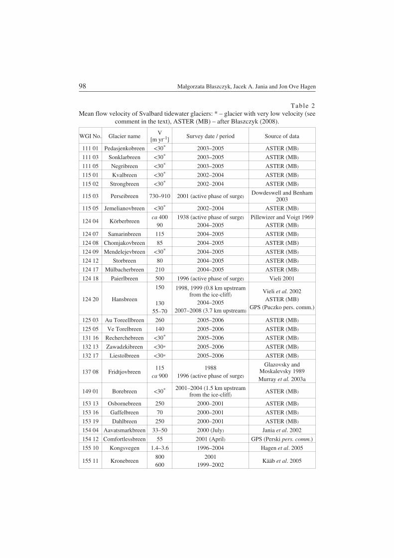
Table 2Mean flow velocity of Svalbard tidewater glaciers: * – glacier with very low velocity (see
comment in the text), ASTER (MB) – after Błaszczyk (2008).
WGI No. Glacier name V[m yr−1] Survey date / period Source of data
111 01 Pedasjenkobreen <30* 2003–2005 ASTER (MB)
111 03 Sonklarbreen <30* 2003–2005 ASTER (MB)
111 05 Negribreen <30* 2003–2005 ASTER (MB)
115 01 Kvalbreen <30* 2002–2004 ASTER (MB)
115 02 Strongbreen <30* 2002–2004 ASTER (MB)
115 03 Perseibreen 730–910 2001 (active phase of surge)Dowdeswell and Benham
2003
115 05 Jemelianovbreen <30* 2002–2004 ASTER (MB)
124 04 Körberbreenca 400
901938 (active phase of surge)
2004–2005Pillewizer and Voigt 1969
ASTER (MB)
124 07 Samarinbreen 115 2004–2005 ASTER (MB)
124 08 Chomjakovbreen 85 2004–2005 ASTER (MB)
124 09 Mendelejevbreen <30* 2004–2005 ASTER (MB)
124 12 Storbreen 80 2004–2005 ASTER (MB)
124 17 Mülbacherbreen 210 2004–2005 ASTER (MB)
124 18 Paierlbreen 500 1996 (active phase of surge) Vieli 2001
124 20 Hansbreen
150
13055–70
1998, 1999 (0.8 km upstreamfrom the ice−cliff)
2004–20052007–2008 (3.7 km upstream)
Vieli et al. 2002ASTER (MB)
GPS (Puczko pers. comm.)
125 03 Au Toreellbreen 260 2005–2006 ASTER (MB)
125 05 Ve Torelbreen 140 2005–2006 ASTER (MB)
131 16 Recherchebreen <30* 2005–2006 ASTER (MB)
132 13 Zawadzkibreen <30* 2005–2006 ASTER (MB)
132 17 Liestolbreen <30* 2005–2006 ASTER (MB)
137 08 Fridtjovbreen115
ca 9001988
1996 (active phase of surge)
Glazovsky andMoskalevsky 1989Murray et al. 2003a
149 01 Borebreen <30* 2001–2004 (1.5 km upstreamfrom the ice−cliff)
ASTER (MB)
153 13 Osbornebreen 250 2000–2001 ASTER (MB)
153 16 Gaffelbreen 70 2000–2001 ASTER (MB)
153 19 Dahlbreen 250 2000–2001 ASTER (MB)
154 04 Aavatsmarkbreen 33–50 2000 (July) Jania et al. 2002
154 12 Comfortlessbreen 55 2001 (April) GPS (Perski pers. comm.)
155 10 Kongsvegen 1.4–3.6 1996–2004 Hagen et al. 2005
155 11 Kronebreen800600
20011999–2002
Kääb et al. 2005

Several previous studies of the velocities of Svalbard glaciers have used thisfeature−tracking method (Lefauconnier et al. 1994; Rolstad et al. 1997; Dowde−swell and Benham 2003; Kääb et al. 2005). However, they only relate to fast−flow−ing and surging−glaciers, and used image pairs acquired only a short time apart.Only Kääb et al. (2005) derived an annual surface velocity field for the lowermost10 km of the fast−flowing Kronebreen. For the present work, the available imageswere of sufficient quality and the time periods between successive ASTER imageacquisitions were long enough that the frontal velocity fields of 27 glaciers couldbe measured for one−year and two−year periods.
The annual surface velocities of glaciers were derived from measurements ofhorizontal displacements of surface features (crevasses, supraglacial moraine ele−ments) that could be unambiguously recognized on successive images. An exam−ple is shown in Fig. 8. In the absence of ground control−points, one ASTER imagewas used as the reference co−ordinate system for a second image. Dowdeswell andBenham (2003) suggested that the velocity error from this source is probablywithin a half to one ASTER pixel (7.5–15 m yr−1). The estimated accuracy of ve−locity measurements derived from repeat ASTER images in this study is probablybetter than ± 30 m yr−1.
For 16 very slow or stagnant tidewater glaciers, very small terminal crevassedareas were noted. For these glaciers there was no measurable surface velocity onASTER images (15 m resolution) in the region near the glacier fronts, even over atwo−years interval (marked with stars in Table 2). Such glaciers are probably in thequiescent phase of a surge cycle.
Tidewater glaciers of Svalbard 99
162 11 Monacobreen 700–800 1995–1996(active phase of surge)
Murray et al. 2003b
172 14 Odinjokulen N <30* 2001–2002 ASTER (MB)
172 15 Tommelbreen <30* 2001–2002 ASTER (MB)
173 02 Sven Ludvigbreen <30* 2001–2002 ASTER (MB)
174 04 Moltkebreen <30* 2003–2006 ASTER (MB)
174 06 Hochstatterbreen <30* 2003–2006 ASTER (MB)
211 08 nameless 238 1995 (winter) Sharov and Etzold 2005
221 02 Palanderbreen 36–49 1996 (winter) Sharov and Etzold 2005
222 08 Aldousbreen 95–142 1996 (winter) Sharov and Etzold 2005
222 09 Frazerbreen 307 1996 (winter) Sharov and Etzold 2005
222 10 Idunbreen 232 1996 (winter) Sharov and Etzold 2005
232 03 S Franklinbreen 35–74 1995/1996 (winter) Sharov and Etzold 2005
232 04 N Franklinbreen 14–49 1995/1996 (winter) Sharov and Etzold 2005
241 03 Sabinebreen <11 1995 (winter) Sharov and Etzold 2005
242 01 Rijpbreen 128 1995 (winter) Sharov and Etzold 2005
251 06 Duvebreen 170–205 1995 (winter) Sharov and Etzold 2005
252 02 Nilsenbreen 84 1995 (winter) Sharov and Etzold 2005

100 Małgorzata Błaszczyk, Jacek A. Jania and Jon Ove Hagen
Fig. 9. Distribution of surges of calving glaciers in Svalbard during last 150 years (cf. Table 3): gla−ciers with registered surge (dots) and glaciers with evidence of surge in their morphology (triangles).
Glacier numbers as used in the inventory (see Appendix) are indicated.

Tidewater glaciers of Svalbard 101
Table 3Registered surges of tidewater glaciers in Svalbard (information sources: Jania 1988a,2006; Lankauf and Wójcik 1987; Lefauconnier and Hagen 1991; Hagen et al. 1993;Rolstad et al. 1997; Dowdeswell et al. 1999; Dowdeswell and Benham 2003; Jania et al.2003; Murray et al. 2003a, b; Kääb et al. 2006; Nuth et al. 2007; Adamek 2007 – personalcomunication); No. – glacier number according to the WGI system (cf. Appendix – Table Iand Figs 12–30), ca – circa, b – between, # – glaciers, which were calving in the past, but
now terminate on land.
No. Glacier name Surgeyear / period No. Glacier name Surge
year / period
111 01 Pedasjenkobreen b. 1925–35 144 03 Tunabreen 1930, 1970,2003–?
111 03 Sonklarbreen ca 1910 147 16 Sefströmbreen 1896
111 05 Negribreen 1935–36 148 05 Wahlenbergbreen 1908
112 01 Hayesbreen 1901 149 02 Nansenbreen 1947
112 06 Ulvebreen b. 1896–1900 153 13 Osbornebreen 1987–90
114 06 Inglefieldbreen 1952 154 04 Aavatsmarkbreen 1982–85
114 07 Arnesenbreen b. 1925–35 155 10 Kongsvegen 1948
114 11 Richardsbreen b. 1990–2002 155 11 Kronebreen 1869
114 12 Thomsonbreen b. 1950–60 155 15 Blomstrandbreen 1960
115 02 Strongbreen b. 1870–76 162 11 Monacobreen ca 1991–97
115 03 Perseibreen 2000–? 172 14 Odinjokulen N b. 1965–70
115 05 Jemelianovbreen 1971 173 05 Kosterbreen ca 1930,b. 1956–70
115 06# Anna Margrethebreen 1970 173 10 Hinlopenbreen 1969–72
115 08 Skimebreen 1970 174 02 Alfarvegen b. 1970–80
115 09 Davisbreen ca 1960 174 06 Hochstatterbreen b. 1895–1900
121 01 Crollbreen b. 1936–61 211 08 nameless b. 1850–1873,1992–94
121 02 Markhambreen b. 1930–36 211 10 Brasvellbreen 1937–38
121 03# Staupbreen ca 1960 221 01 Glitnefonna Ne 1938
121 04 Hambergbreen ca 1890, ca 1960 221 02 Palanderbreen 1969–70
122 02 Vasilievbreen ca 1961 222 03 Etonbreen 1938
124 04 Körberbreen 1938, ca 1960 222 06 Bodleybreen 1973–80
124 09 Mendelejevbreen ca 2000 232 03 S Franklinbreen 1956
124 18 Paierlbreen 1993–99 242 01 Rijpbreen 1938, 1992
131 16 Recherchebreen 1838, 1945 313 18 Stonebreen b. 1936 – 1971,b. 1850–60
132 13 Zawadzkibreen 2006–? 313 19 Kong Johans Bre b. 1925–1930
134 10# Bakaninbreen 1985–90 321 01 Freemanbreen 1955–56
137 08 Fridtjovbreen 1861, ca 1991–97 321 02 Duckwitzbreen 1918
144 02 # Von Postbreen 1870, 1980

Glacier surges are an important element of the dynamics of many Svalbard icemasses. In the active phase of a surge, the ice flow velocity increases by several or−ders of magnitude. Fast down−glacier transfer of ice is observed, the glacier surfacebecomes badly crevassed (cf. Fig. 10d), and frontal advance is often noted (Meierand Post 1969). After a surge, glaciers may stagnate for periods of decades or evencenturies. Thinning of the glacier tongue and frontal retreat have commonly beenobserved during the quiescent phase of a surge cycle.
The active phase of surging affects the ice flux from tidewater glaciers (cf. Ta−ble 2) and the calving rate is naturally increased. Based on published data, 55 tide−water glaciers (33% of all tidewater glaciers) have been considered as surge−type(Table 3, Fig. 9). However, a new approach to the evaluation of the number ofsurge−type glaciers within the population of Svalbard tidewater glaciers has beenmade in this study. On the basis of publications, unpublished reports, personalcommunications and interpretations of aerial photographs and satellite images(e.g. folded foliation and looped medial moraines visible on glacier surfaces), up to43% of Svalbard tidewater glaciers could be classified as surge type (Fig. 9). Theseglaciers were probably actively surging at some time during the 20th century.
Iceberg calving from Svalbard glaciers
The calculation of the volume of ice lost by calving of icebergs from a tidewa−ter glacier is possible when the following quantities are known: (1) the velocity ofthe glacier averaged over the cross sectional area of the glacier terminus, (2)ice−cliff area, (3) glacier front advance or retreat. It can be described by:
Q V C H X C HC � � � � � � (1)
where: Qc is the volumetric flux of icebergs, V is the mean ice flow velocity, C isthe cliff length, H is the ice thickness and X is front retreat (positive) or advance(negative).
The estimation of iceberg production from the whole Svalbard archipelago re−quires these data for every tidewater glacier on the archipelago but we have no dataof any kind for most glaciers. Therefore, we have tried to approximate the annualrate of ice movement from the pattern and size of the zone of crevasses on eachtidewater glacier in Svalbard.
Our classification of tidewater glaciers according to their dynamics is based onthe size of the crevassed zone close to the glacier termini. A relationship betweenglacier velocity and the occurrence of crevasses was used to estimate the dynamicsof all tidewater glaciers in Svalbard. This approach is predicted upon a simple as−sumption: when glacier speed is high, more crevasses are noted in the frontal partof a glacier and the area of crevassing is larger (i.e. a fast glacier produces a largercrevasse system near its front).
102 Małgorzata Błaszczyk, Jacek A. Jania and Jon Ove Hagen

Crevasses on tidewater glaciers are generally parallel or semi−parallel to theice−cliff and their origin is related to the increase of tensile stresses in the lowerreaches of the glacier (cf. Van der Veen 1999), as longitudinal gradient in flow ve−locity rises when the ice approaches the glacier terminus. Although undulations inthe underlying bedrock surface may influence the size and pattern of a crevassefield to some extent, flow velocity is assumed to be the primary influence. In activephase of a surge cycle, a substantial part of glacier is usually heavily crevassed (cf.Fig. 10d).
As linear features, crevasses are easily identified on the surface of glaciers reg−istered on Terra−ASTER satellite images (even when their width is less than 15 m).It is possible to define the distribution and patterns of crevasses semi−automati−
Tidewater glaciers of Svalbard 103
Fig. 10. Examples of ASTER geocoded images (321 bands) of glaciers classified into differentgroups of flow dynamics: a) Negribreen – very slow or stagnant glacier (5.08.2003); b) Storbreen –slow−flowing glacier (7.08.2004); c) Austre Torellbreen – fast−flowing glacier (23.07.2005);
d) Perseibreen – active surge glacier (7.08.2004).

cally using the remote sensing texture analysis (MaZda, cf. Fig. 4b) and GIS soft−ware (e−Cognition, ArcGIS) supported by manual digitization of crevassed areas.
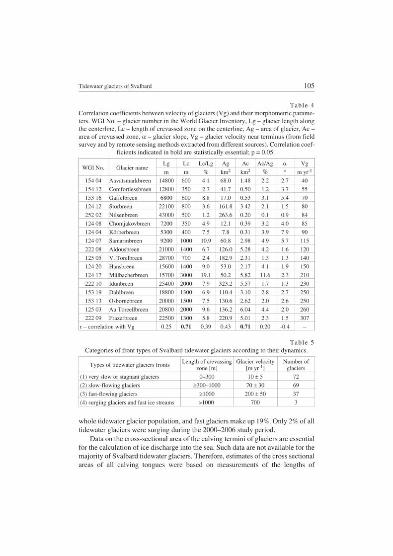
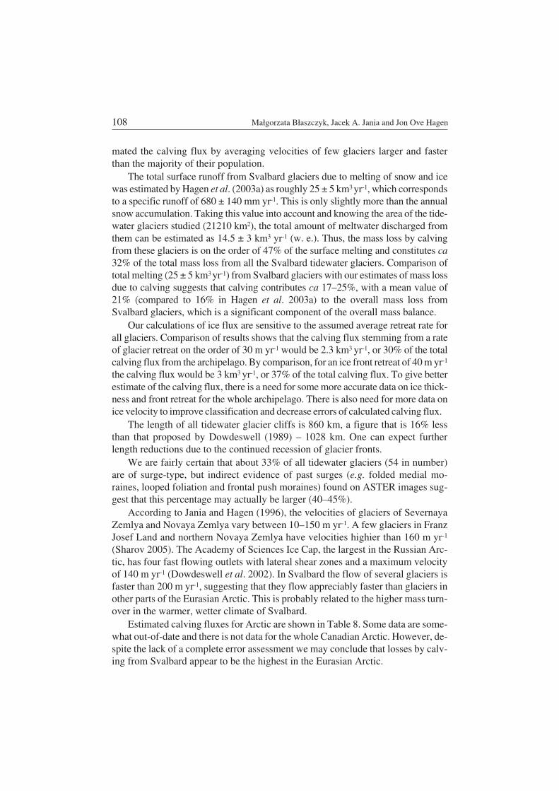
Data on the near terminus velocity of different types of glaciers were requiredfor classification of glaciers according to their dynamics. Flow velocity measure−ments for 46 glaciers were obtained (Table 2). From these measurements madeover the last two decades we used velocity data from only 33 glaciers. Analysis ofthe dynamic status of tidewater glaciers was based on several characteristics:length of glacier, length of crevassed zone, area of glacier, area of crevassed zoneand length of cliff, as acquired from satellite imagery. Owing to the difficultieswith determining of crevasses zone due to snow cover on glacier front, some of thevelocity information was rejected. 16 apparently stagnant glaciers that currentlyhave very small crevassed areas and no discernible motion (cf. Table 2) fall intofirst category of “very slow or stagnant glaciers”. The morphometric features of afurther 17 glaciers were compared with their mean annual flow velocity (Table 4).
The highest correlation coefficient (r = 0.71) was found between 17 glacier ve−locities and the length and area of crevassed zones. In practice, it is easier to measurethe linear extent of the crevassed zone upstream from the ice−cliff along the center−line than to measure its area. A multiple regression with use of both parameters,length and area of crevassed zones, was also calculated, but correlation coefficient ofregression equation was too low (r = 0.56). Therefore parameter “length of thecrevassed zone” was used for further velocity and calving flux assessments. In orderto estimate the velocities of all the tidewater glaciers in the archipelago, the glacierswere classified into four groups with different dynamics (Table 5): (1) very slow orstagnant glaciers with velocities (Vg) in the range 10 ± 5 m yr−1 and length ofcrevassed zone (Lc) of 0–300 m, (2) slow−flowing glaciers with Vg of 70 ± 30 m yr−1
and Lc of 300–1000 m, (3) fast−flowing glaciers with Vg of 200 ± 50 m yr−1 and Lc of� 1000 m, (4) surging glaciers (in the active phase) and fast ice streams with Vg > ca700 m yr−1 and Lc of a few kilometers. Ranges (estimated errors) in velocities in indi−vidual groups are assumed on the basis of sparse data on glacier motion. Examplesof the different dynamic categories of glaciers are presented in Fig. 10.
Every tidewater glacier on Svalbard was assigned to one of the above groupsand an average velocity for a given dynamic type was applied to all glaciers of thattype. Special attention was paid to those glaciers that have recently surged. Theirsurfaces are heavily crevassed but they are slow moving or even stagnant. Thus,every glacier with traces of a surge on its surface was examined individually by ap−plying the feature tracking method to ASTER images from different years to deter−mine its velocity. Other sources of data (publications, unpublished information)were also used for this purpose.
The classification presented allowed us to approximate the average flow ve−locity of every tidewater glacier in the archipelago on the basis of length of thecrevassed zone. As a result of classification, very slow or stagnant glaciers consti−tute 49% of Svalbard tidewater glaciers, while slow glaciers make up 30% of the
104 Małgorzata Błaszczyk, Jacek A. Jania and Jon Ove Hagen
whole tidewater glacier population, and fast glaciers make up 19%. Only 2% of alltidewater glaciers were surging during the 2000–2006 study period.
Data on the cross−sectional area of the calving termini of glaciers are essentialfor the calculation of ice discharge into the sea. Such data are not available for themajority of Svalbard tidewater glaciers. Therefore, estimates of the cross sectionalareas of all calving tongues were based on measurements of the lengths of
Tidewater glaciers of Svalbard 105
Table 4Correlation coefficients between velocity of glaciers (Vg) and their morphometric parame−ters. WGI No. – glacier number in the World Glacier Inventory, Lg – glacier length alongthe centerline, Lc – length of crevassed zone on the centerline, Ag – area of glacier, Ac –area of crevassed zone, � – glacier slope, Vg – glacier velocity near terminus (from fieldsurvey and by remote sensing methods extracted from different sources). Correlation coef−
ficients indicated in bold are statistically essential; p = 0.05.
WGI No. Glacier nameLg Lc Lc/Lg Ag Ac Ac/Ag � Vg
m m % km2 km2 % � m yr−1
154 04 Aavatsmarkbreen 14800 600 4.1 68.0 1.48 2.2 2.7 40
154 12 Comfortlessbreen 12800 350 2.7 41.7 0.50 1.2 3.7 55
153 16 Gaffelbreen 6800 600 8.8 17.0 0.53 3.1 5.4 70
124 12 Storbreen 22100 800 3.6 161.8 3.42 2.1 1.5 80
252 02 Nilsenbreen 43000 500 1.2 263.6 0.20 0.1 0.9 84
124 08 Chomjakovbreen 7200 350 4.9 12.1 0.39 3.2 4.0 85
124 04 Körberbreen 5300 400 7.5 7.8 0.31 3.9 7.9 90
124 07 Samarinbreen 9200 1000 10.9 60.8 2.98 4.9 5.7 115
222 08 Aldousbreen 21000 1400 6.7 126.0 5.28 4.2 1.6 120
125 05 V. Torelbreen 28700 700 2.4 182.9 2.31 1.3 1.3 140
124 20 Hansbreen 15600 1400 9.0 53.0 2.17 4.1 1.9 150
124 17 Mülbacherbreen 15700 3000 19.1 50.2 5.82 11.6 2.3 210
222 10 Idunbreen 25400 2000 7.9 323.2 5.57 1.7 1.3 230
153 19 Dahlbreen 18800 1300 6.9 110.4 3.10 2.8 2.7 250
153 13 Osbornebreen 20000 1500 7.5 130.6 2.62 2.0 2.6 250
125 03 Au Toreellbreen 20800 2000 9.6 136.2 6.04 4.4 2.0 260
222 09 Frazerbreen 22500 1300 5.8 220.9 5.01 2.3 1.5 307
r – correlation with Vg 0.25 0.71 0.39 0.43 0.71 0.20 −0.4 –
Table 5Categories of front types of Svalbard tidewater glaciers according to their dynamics.
Types of tidewater glaciers fronts Length of crevassingzone [m]
Glacier velocity[m yr−1]
Number ofglaciers
(1) very slow or stagnant glaciers 0–300 10 � 5 72
(2) slow−flowing glaciers �300–1000 70 � 30 69
(3) fast−flowing glaciers �1000 200 � 50 37
(4) surging glaciers and fast ice streams >1000 700 3

ice−cliffs and assumptions about the mean thickness of glaciers in contact with seawater. The length of all tidewater glacier cliffs was measured using geocoded AS−TER images (Table 6). This amounts to 860 km, a figure which is 16% shorter thanthat proposed by Dowdeswell (1989) – 1028 km. This may simply reflect reduc−tion of seaward margins of tidewater glaciers in around last 40 years.
The average ice thickness near the terminus was estimated from airborne andground−based radio echo soundings of some dozens of glaciers and from the verysparse data on ocean depth close to the present ice front positions (Dowdeswell etal. 1984; Drewry and Liestøl 1985; Hagen et al. 2003a). From this data averagethickness of glacier fronts in the archipelago is estimated to be about 100 m ± 10 m.
An extensive analysis of images has enabled us to obtain other data necessaryto estimate the annual calving flux of ice from Svalbard glaciers to the ocean in thefirst years of the 21st century. The calving loss from glaciers with stable ice frontpositions was estimated to be about 5.2 km3 yr−1 ± 1.5 km3 yr−1 (Table 7).
Terminus position changes of about 30 tidewater glaciers were measured and,for the purposes of calculation of the calving flux, an average retreat rate by
106 Małgorzata Błaszczyk, Jacek A. Jania and Jon Ove Hagen
Table 6The length of ice cliffs on the main islands of Svalbard: L1 – Dowdeswell (1989); L2 – from
ASTER satellite images.
IslandLength of ice cliffs
L1 [km] L2 [km]Spitsbergen 484 388.4
Nordaustlandet 306 272.3
Edgeøya 79 68.7
Prins Karls Forland 17 8.9
Barentsøya 23 8.8
Storøya 13 12
Kvitøya 106 100
Sum 1028 km 859.1 km
Table 7The calving losses from different types of glacier (without taking into the consideration re−cession of termini); Qc – mean annual calving flux; Qc – sum of calving estimation errors
with assumption of a stable front position.
Types of tidewater glaciers Qc[km3 yr−1]
Qc[km3 yr−1]
(1) very slow or stagnant glaciers 0.4 0.2(2) slow−flowing glaciers 1.8 0.8(3) fast−flowing glaciers 2 0.5(4) surging glaciers and fast ice streams 1 –Total for Svalbard 5.2 1.5

30 m yr−1 was assigned to the whole population. Taking into account the mean re−cession rate of all the tidewater glaciers, the total length of ice−cliffs (860 km) andthe average thickness of glaciers at the terminus (100 m), the additional calving iceflux as a result of glacier retreat was estimated to be 2.28 km3 yr−1. The total calvingflux from Svalbard glaciers (excluding Kvitøya) was estimated to be 7.5 km3 yr−1.
Overall uncertainty on the calving flux is derived assuming: average ice thick−ness of 100 m ± 10 m, mean ice flow velocity and error of velocity according to Ta−ble 5, the average front retreat of 30 m yr−1 ± 10 m yr−1, the cliff length from Table I(Appendix) and error of the cliff length of ±15 m. These quantities are the best pos−sible values based on our observations. Sum of individual errors of calving flux ofall glaciers amounts to 1.9 km3 yr−1.
Thus, the total calving flux from Svalbard glaciers was estimated to be in therange 5.6–9.4 km3 yr−1 of ice (5.0–8.4 km3 yr−1 water equivalent – w.e.) with thebest estimate of 7.5 ± 1.9 km3 yr−1 (6.75 ± 1.7 km3 yr−1 w.e.).
Discussion and conclusions
The present analysis of tidewater glaciers in Svalbard is based on examination ofASTER satellite images from the period 2000–2006, while data in Hagen’s et al.(1993) inventory were collected from sources of different origin and age. Recentdata have shown that there are 163 tidewater glaciers in Svalbard. Compared to theprevious inventory, 14 glaciers have retreated from the sea to land during the last30–40 years, and 11 formerly land−based glaciers are now in contact with the sea.
In this inventory, tidewater glaciers were classified into four groups on the ba−sis of their dynamic state and frontal crevasse patterns: (1) very slow or stagnantglaciers, (2) slow−flowing glaciers, (3) fast−flowing glaciers, (4) surging glaciers(in the active phase) and fast ice streams.
Our estimates of total mass loss due to calving from Svalbard glaciers (exclud−ing Kvitøya) yield values of 5.0–8.4 km3 yr−1 (w.e.) with the best estimate being6.75 ± 1.7 km3 yr−1 (w.e.), which is substantially more than the calving flux of 4 ± 1km3 yr−1 (w.e.) given by Hagen et al. (2003a) and significantly less than the valueestimated by Lefauconnier et al. (1993), 7.44–9.94 km3 yr−1.
The differences between these estimates stem from assuming general velocityfor the whole archipelago. Hagen et al. (2003a) estimated the average velocity ofcalving fronts through the archipelago at 20–40 m yr−1, and general retreat of gla−cier fronts at 10 m yr−1. Lefauconnier et al. (1993) calculated linear calving (flowvelocity plus retreat of the front) on 75 m per year for Spitsbergen and 100 metersper year for the islands of the eastern Svalbard. Therefore, Hagen et al. (2003a) re−sult is smaller because they assumed too low velocity for all Svalbard glaciers. Re−sults of Lefauconnier et al. (1993) are giving too high values, because they esti−
Tidewater glaciers of Svalbard 107
mated the calving flux by averaging velocities of few glaciers larger and fasterthan the majority of their population.
The total surface runoff from Svalbard glaciers due to melting of snow and icewas estimated by Hagen et al. (2003a) as roughly 25 ± 5 km3 yr−1, which correspondsto a specific runoff of 680 ± 140 mm yr−1. This is only slightly more than the annualsnow accumulation. Taking this value into account and knowing the area of the tide−water glaciers studied (21210 km2), the total amount of meltwater discharged fromthem can be estimated as 14.5 ± 3 km3 yr−1 (w. e.). Thus, the mass loss by calvingfrom these glaciers is on the order of 47% of the surface melting and constitutes ca32% of the total mass loss from all the Svalbard tidewater glaciers. Comparison oftotal melting (25 ± 5 km3 yr−1) from Svalbard glaciers with our estimates of mass lossdue to calving suggests that calving contributes ca 17–25%, with a mean value of21% (compared to 16% in Hagen et al. 2003a) to the overall mass loss fromSvalbard glaciers, which is a significant component of the overall mass balance.
Our calculations of ice flux are sensitive to the assumed average retreat rate forall glaciers. Comparison of results shows that the calving flux stemming from a rateof glacier retreat on the order of 30 m yr−1 would be 2.3 km3 yr−1, or 30% of the totalcalving flux from the archipelago. By comparison, for an ice front retreat of 40 m yr−1
the calving flux would be 3 km3 yr−1, or 37% of the total calving flux. To give betterestimate of the calving flux, there is a need for some more accurate data on ice thick−ness and front retreat for the whole archipelago. There is also need for more data onice velocity to improve classification and decrease errors of calculated calving flux.
The length of all tidewater glacier cliffs is 860 km, a figure that is 16% lessthan that proposed by Dowdeswell (1989) – 1028 km. One can expect furtherlength reductions due to the continued recession of glacier fronts.
We are fairly certain that about 33% of all tidewater glaciers (54 in number)are of surge−type, but indirect evidence of past surges (e.g. folded medial mo−raines, looped foliation and frontal push moraines) found on ASTER images sug−gest that this percentage may actually be larger (40–45%).
According to Jania and Hagen (1996), the velocities of glaciers of SevernayaZemlya and Novaya Zemlya vary between 10–150 m yr−1. A few glaciers in FranzJosef Land and northern Novaya Zemlya have velocities highier than 160 m yr−1
(Sharov 2005). The Academy of Sciences Ice Cap, the largest in the Russian Arc−tic, has four fast flowing outlets with lateral shear zones and a maximum velocityof 140 m yr−1 (Dowdeswell et al. 2002). In Svalbard the flow of several glaciers isfaster than 200 m yr−1, suggesting that they flow appreciably faster than glaciers inother parts of the Eurasian Arctic. This is probably related to the higher mass turn−over in the warmer, wetter climate of Svalbard.
Estimated calving fluxes for Arctic are shown in Table 8. Some data are some−what out−of−date and there is not data for the whole Canadian Arctic. However, de−spite the lack of a complete error assessment we may conclude that losses by calv−ing from Svalbard appear to be the highest in the Eurasian Arctic.
108 Małgorzata Błaszczyk, Jacek A. Jania and Jon Ove Hagen

The contribution of Svalbard iceberg flux to sea−level rise may be as much as0.02 mm yr−1 and it is certainly greater than the value of 0.01 mm yr−1 presented byHagen et al. (2003a). Although it is a small part of the total sea−level rise from gla−ciers and ice caps (estimated at 1.1 mm yr−1; Meier et al. 2007) and minuscule com−pared with the contributions of Greenland to sea−level rise (0.5 mm yr−1; Rignotand Kanagaratnam 2006), the annual specific mass loss due to calving from theSvalbard Archipelago appears to be the largest in the Arctic (Fig. 11). One mayreasonably predict that some present−day tidewater glaciers will retreat to the land
Tidewater glaciers of Svalbard 109
0
0.05
0.10
0.15
0.20
0.25
Sva
lba
rd
Fra
nz
Jo
se
fL
an
d
Se
ve
rna
ya
Ze
mly
a
No
va
ya
Ze
mly
a
Gre
en
lan
d
De
vo
nIc
eC
ap
Elle
sm
ere
Isla
nd
Fig. 11. Annual specific mass balance attributable to the calving flux (calving flux/area) [m yr−1].
Table 8Estimations of volume of ice lost by calving in Eurasian and North Atlantic Arctic area(data sources: 1 Błaszczyk 2008, 2 Govorukha 1989, 3 Abramov 1996, 4 Dowdeswell et al.2002, 5 Rignot and Kanagaratnam 2006, 6 Burgess et al. 2005, 7 Willamson et al. 2008,
8 Short and Gray 2005, 9 http://nsidc.org/data/docs/noaa/g01130_glacier_inventory/).
Island Calving flux[km3 yr−1]
Glaciers area[km2]
Annual specific mass balanceattributable to iceberg calving
[m yr−1]
Svalbard1 7.5 36 600 0.20
Novaya Zemlya2 2 23 600 0.087
Franz Josef Land3 2.26 13 700 0.16
Academy of Sciences Ice Cap(Severnaya Zemlya)4
0.65 5 500 0.12
Greenland5 150 1 640 000 0.09
Devon Ice Cap (Devon Island)6 0.53 14 000 0.04
Agassiz Ice Cap7
Otto Glacier7
Prince of Wales Icefield8
(Ellesmere Island)
0.67 � 0.150.26 � 0.132.81 � 0.69
19 5002 0001 3709
0.030.132.05
and that the lengths of the remaining ice cliffs will be reduced. Therefore, in thecoming decades, a decrease in the calving flux may be expected.
In conclusion, we suggest that area and pattern of crevasses near tidewater gla−cier termini seems to be a simple and reliable indicator of the dynamics of theseglaciers. It also enables the estimation of the likely flow velocity and calving fluxof individual glaciers in Svalbard.
Acknowledgements. — These studies were financed by the Ministry of Science and HigherEducation, Republic of Poland under terms of the special research grant No. IPY−269/2006(PL−GLACIODYN), coordinated by JAJ. This work was also supported by the Rector of theUniversity of Silesia (BW−JMR grant for JAJ). The ASTER data were received by the distribu−tion of the Land Processes Distributed Active Archive Center (LP DAAC), by the U.S.Geologi−cal Survey Earth Resources Observation and Science (EROS) Center (lpdaac.usgs.gov). Wethank in particular Dr. Leszek Kolondra and Dr. Wojciech Drzewiecki for discussions on meth−ods and Dr. Habil. Peter T. Walsh for his linguistic assistance. Valuable remarks by ProfessorMartin Sharp are greatly appreciated.
References
ACIA 2005. Arctic Climate Impact Assessment. Cambridge University Press, Cambridge: 1460 pp.ABRAMOV V.A. 1996. Atlas of Arctic Icebergs, The Greenland, Barents, Kara, Laptev, East−Sibe−
rian seas, and the Arctic Basin. Backbone Publishing Company, NJ: 70 pp.BŁASZCZYK M. 2008. Zastosowanie metod teledetekcyjnych dla określenia intensywności cielenia lo−
dowców Svalbardu. Unpublished Ph.D. thesis. University of Silesia, Sosnowiec: 196 pp. (in Polish)BOLCH T., BUCHROITHNER M., PIECZONKA T. and KUNERT A. 2008. Planimetric and volumetric
glacier changes in the Khumbu Himal, Nepal, since 1962 using Corona, Landsat TM andASTER data. Journal of Glaciology 54 (187): 592–600.
BURGESS D.O., SHARP M., MAIR D.W.F., DOWDESWELL J.A. and BENHAM T.J. 2005. Flow dynam−ics and iceberg calving rates of the Devon Ice Cap, Nunavut, Canada. Journal of Glaciology 51(173): 219–230.
CARLSEN M., HAGEN J.O. and LØNNE I. 2003. Glacier front retreat in Van Keulenfjorden, Svalbard,during the last 100 years. In: S. Bondevik, M. Hald, E. Isaksson, N. Koc and T. Vorren (eds)33rd Annual Arctic Workshop Polar Environmental Centre, Tromsø, Norway, 3–5 April 2003.Norsk Polarinstitutt Internrapport 13: 63.
DOWDESWELL J.A. 1989. On the nature of Svalbard icebergs. Journal of Glaciology 35 (120): 224–234.DOWDESWELL J.A. 2006. The Greenland Ice Sheet and Global Sea−Level Rise. Science 311 (5763):
963–964.DOWDESWELL J.A. and BENHAM T.J. 2003. A surge of Perseibreen, Svalbard, examined using aerial
photography and ASTER high−resolution satellite imagery. Polar Research 22 (2): 373–383.DOWDESWELL J.A. and HAGEN J.O. 2004. Arctic ice masses. Chapter 15. In: J.L. Bamber and A.J.
Payne (eds) Mass Balance of the Cryosphere. Cambridge University Press, Cambridge: 644 pp.DOWDESWELL J.A., HAGEN J.O., GLAZOVSKY A. and JANIA J. 2001. GISICE – Glaciological Data−
base of the Eurasian High Arctic. CD. University of Bristol, UK.DOWDESWELL J.A. and HAMBREY M. 2002. Islands of the Arctic. Cambridge University Press,
Cambridge: 280 pp.DOWDESWELL J.A., BASSFORD R.P., GORMAN M.R., WILLIAMS M., GLAZOVSKY A.F., MACHERET
Y.Y., SHEPHERD A.P., VASILENKO Y.V., SAVATYUGUIN L.M., HUBBERTEN H.−W. and MILLER
H. 2002. Form and flow of the Academy of Sciences Ice Cap, Severnaya Zemlya, Russian HighArctic. Journal of Geophysical Research 107, 2076, doi:10.1029/2000/JB000129.
110 Małgorzata Błaszczyk, Jacek A. Jania and Jon Ove Hagen
DOWDESWELL J.A., BENHAM T. J., STROZZI T. and HAGEN J.O. 2008. Iceberg calving flux and massbalance of the Austfonna ice cap on Nordaustlandet, Svalbard. Journal of Geophysical Research113, F03022, doi:10.1029/2007JF000905.
DOWDESWELL J.A., DREWRY D.J., LIESTØL O. and ORHEIM O. 1984. Airborne radio echo soundingof sub−polar glaciers in Spitsbergen. Norsk Polarinstitutt Skrifter 182: 42 pp.
DOWDESWELL J.A., HAMILTON G. and HAGEN J.O. 1991. The duration of the active phase onsurge−type glaciers: contrasts between Svalbard and other regions. Journal of Glaciology 37(127): 86–98.
DOWDESWELL J.A., UNWIN A., NUTTALL M. and WINGHAM D.J. 1999. Velocity structure, flow in−stability and mass flux on a large Arctic ice cap from satellite radar interferometry. Earth andPlanetary Science Letters 167 (3): 131–140.
DREWRY D.J. and LIESTØL O. 1985. Glaciological investigations of surging ice caps in Nordaust−landet, Svalbard, 1983. Polar Record 22 (139): 357–378.
GLAZOVSKY A.F. and MOSKALEVSKY M.Y. 1989. Issledovaniya lednika Fritiof na Shpitsbergene v1988 godu. Materialy Glyatsiologicheskikh Issledovaniy 65: 148–152. (in Russian)
GŁOWACKI P. and JANIA J.A. 2008. Nature of rapid response of glaciers to climate warmingin South−ern Spitsbergen, Svalbard. In: Drastic Change under the Global Warming. Extended abstracts,The First International Symposium on the Arctic Research – ISAR−1, Tokyo: 257–260.
GOVORUKHA L.S. 1989. Modern glaciation of the Soviet Arctic. Hydrometeoizdat, Leningrad: 256 pp.GRZEŚ M., KRÓL M. and SOBOTA I. 2008. Glacier geometry change in the Forlandsundet area (NW
Spitsbergen) using remote sensing data. In: C.H. Tijm−Reijmer (ed.) The Dynamics and MassBudget of Arctic Glaciers. Extended abstracts. Workshop and GLACIODYN (IPY). 29–31 Janu−ary 2008, Obergurgl (Austria). IASC Working group on Arctic Glaciology: 50–52.
HAGEN J.O., EIKEN T., KOHLER J. and MELVOLD K. 2005. Geometry changes on Svalbard glaciers:mass−balance or dynamic response? Annals of Glaciology 42: 255–261.
HAGEN J.O., LIESTØL O., ROLAND E. and JØRGENSEN T. 1993. Glacier Atlas of Svalbard and JanMayen. Norsk Polarinstitutt Meddelelser 129, Oslo: 141 pp.
HAGEN J.O., MELVOLD K., PINGLOT F. and DOWDESWELL J.A. 2003a. On the Net Mass Balance ofthe Glaciers and Ice Caps in Svalbard, Norwegian Arctic. Arctic, Antarctic, and Alpine Research35 (2): 264–270.
HAGEN J.O., KOHLER J., MELVOLD K. and WINTHER J.G. 2003b. Glaciers in Svalbard: mass bal−ance, runoff and freshwater flux. Polar Research 22 (2): 145–159.
HARALICK R.M., SHANMUGAN K. and DINSTEIN I. 1973. Textural Features for Image Classification.IEEE Transaction on Systems, Man and Cybernetics 3: 610–621.
IPCC 2007. Climate Change 2007: The Physical Science Basis. Contribution of Working Group I tothe Fourth Assessment. Report of the Intergovernmental Panel on Climate Change. CambridgeUniversity Press, United Kingdom and New York, NY.
JANIA J. 1988a. Dynamiczne procesy glacjalne na południowym Spitsbergenie (w świetle badań foto−interpretacyjnych i fotogrametrycznych). Prace Naukowe Uniwersytetu Śląskiego w Katowicach,Katowice: 258 pp. (in Polish)
JANIA J. 1988b. Klasyfikacja i cechy morfometryczne lodowców otoczenia Hornsundu, Spitsbergen.In: J. Jania and M. Pulina (eds) Wyprawy Polarne Uniwersytetu Śląskiego 1980–1984, t. 2,Uniwersytet Śląski, Katowice: 12–47. (in Polish)
JANIA J. 2002. Calving intensity of Spitsbergen glaciers. In: J.B. Ørbæk, K. Holmén, R. Neuber, H.P.Plag, B. Lefauconnier, G. Prisco and H. Ito (eds) The Changing Physical Environment. Proceed−ings from the Sixth Ny−Ålesund International Scientific Seminar. Tromsø, Norway, 8–10 Octo−ber 2002. Norsk Polarinstitutt, Internrapport 10: 117–120.
JANIA J. 2006. Charakter i skala zmian pokrywy zlodowacenia w Arktyce. Konferencja Zmianyklimatyczne w Arktyce i Antarktyce w ostatnim pięćdziesięcioleciu XX wieku i ich implikacjeśrodowiskowe. 11–13 maja 2006. Program, Abstrakty, Akademia Morska, Gdynia, http://ocean.am.gdynia.pl/sem/konf−global.html (in Polish)
Tidewater glaciers of Svalbard 111

JANIA J. and HAGEN J.O. (eds) 1996. Mass Balance of Arctic Glaciers. IASC Report 5, University ofSilesia, Sosnowiec–Oslo: 62 pp.
JANIA J., GŁOWACKI P., KOLONDRA L., PERSKI Z., PIWOWAR B., PULINA M., SZAFRANIEC J.,BUKOWSKA−JANIA E. and DOBIŃSKI W. 2003. Lodowce otoczenia Hornsundu. In: A. Kostrzewskiand Z. Zwoliński (eds) Funkcjonowanie dawnych i współczesnych geoekosystemów Spitsbergenu.Stowarzyszenie Geomorfologów Polskich, Poznań–Longyearbyen: 190 pp. (in Polish)
JANIA J., PERSKI Z. and STOBER M. 2002. Changes of geometry and dynamics of NW Spitsbergenglaciers based on the ground GPS survey and remote sensing. In: J.B. Ørbæk, K. Holmén, R.Neuber, H.P. Plag, B. Lefauconnier, G. Prisco and H. Ito (eds) The Changing Physical Environ−ment. Proceedings from the Sixth Ny−Ålesund International Scientic Seminar, Tromsø, Norway,8–10 October 2002. Norsk Polarinstitutt Internrapport 10: 137–140.
JISKOOT H., MURRAY T. and BOYLE P. 2000. Controls on the distribution of surge−type glaciers inSvalbard. Journal of Glaciology 46 (154): 412–422.
KÄÄB A. 2005. Remote Sensing of Mountain Glaciers and Permafrost Creep. Physical GeographySeries 48. University of Zürich, Zürich: 264 pp.
KÄÄB A., HAGEN J.O., HUMLUM O., CHRISTIANSEN H., KRISTENSEN L. and BENN D. 2006. Recentglacier surges in Svalbard measured from repeat ASTER satellite optical stereo images. Geo−physical Research Abstracts 8, European Geosciences Union.
KÄÄB A., LEFAUCONNIER B. and MELVOLD K. 2005. Flow field of Kronebreen, Svalbard, using re−peated Landsat7 and ASTER data. Annals of Glaciology 42: 7–13.
KORYAKIN V.S. 1975. Kolebanya lednikov. In: L.S. Troitsky, E.M. Singer, V.S. Koryakin, V.A.Markin and V.I. Mikhaliov (eds) Oledenenyie Spitsbergena (Svalbarda). Nauka, Moskva:165–184. (in Russian)
LANKAUF K.R. and WÓJCIK G. 1987. Zmiany zasięgu czół lodowców Ziemi Oskara II (NWSpitsbergen). Wyniki badań VIII Toruńskiej Wyprawy Polarnej Spitsbergen '89. UMK Toruń:113–129. (in Polish)
LEFAUCONNIER B. and HAGEN J.O. 1991. Surging and calving glaciers in Eastern Svalbard. NorskPolarinstitutt Meddelelser 116, Oslo: 130 pp.
LEFAUCONNIER B., HAGEN J.O. and RUDANT J.P. 1994. Flow speed and calving rate of Kronebreenglacier, Svalbard, using SPOT images. Polar Research 13 (1): 59–65.
LEFAUCONNIER B., VALLON M., DOWDESWELL J., HAGEN J.O., PINGLOT J.F. and PURCHET M.1993. Global balance of Spitsbergen ice masses and prediction of its change due to climaticchange. EPOCH 0035 Scientific Report: 18 pp.
LIESTØL O. 1969. Glacier surges in West Spitsbergen. Canadian Journal of Earth Sciences 6 (4):895–987.
LIESTØL O. 1973. Glaciological work in 1971. Norsk Polarinstitutt Årbok 1971, Oslo: 67–76.LØNNE I. 2003. Fridtjovbreen on Svalbard – evolution of the two last surge events. In: S. Bondevik,
M. Hald, E. Isaksson, N. Koc and T. Vorren (eds) 33rd Annual Arctic Workshop Polar Environ−mental Centre, Tromsø, Norway 3–5 April 2003. Norsk Polarinstitutt Internrapport 13: 42.
MEIER M.F. and POST A.S. 1969. What are glacier surges? Canadian Journal of Earth Sciences 6:807–817.
MEIER M.F., DYURGEROV M.B., RICK U.K., O'NEEL S., PFEFFER W.T., ANDERSON R.S., ANDERSON
S.P. and GLAZOVSKY A.F. 2007. Glaciers dominate eustatic sea−level rise in the 21st century. Sci−ence 317 (5841): 1064–1067.
MOLNIA B.F. 2008. Glaciers of North America – Glaciers of Alaska. In: R.S. Williams, Jr and J.G.Ferrigno (eds) Satellite image atlas of glaciers of the world. U.S. Geological Survey Profes−sional Paper 1386−K: 525 pp.
MURRAY T., LUCKMAN A., STROZZI T. and NUTTALL A.M. 2003a. The initiation of glacier surgingat Fridtjovbreen, Svalbard. Annals of Glaciology 36: 110–116.
MURRAY T., STROZZI T., LUCKMAN A., JISKOOT H. and CHRISTAKOS P. 2003b. Is there a singlesurge mechanism?: Contrast in dynamics between glacier surges in Svalbard and other regions.Journal of Geophysical Research 108 (B5), 2237, doi:10.1029/2002JB001906.
112 Małgorzata Błaszczyk, Jacek A. Jania and Jon Ove Hagen

NETTLES M., LARSEN T.B., ELÓSEGUI P., HAMILTON G.S., STEARNS L.A., AHLSTRØM A.P.,DAVIS J.L., ANDERSEN M.L., DE JUAN J., KHAN S.A., STENSENG L., EKSTRÖM G. andFORSBERG R. 2008. Step−wise changes in glacier flow speed coincide with calving and gla−cial earthquakes at Helheim Glacier, Greenland. Geophysical Research Letters 35, L24503,doi:10.1029/2008GL036127.
NUTH C., KOHLER J., AAS H.F., BRANDT O. and HAGEN J.O. 2007. Glacier geometry and elevationchanges on Svalbard (1936–90): a baseline dataset. Annals of Glaciology 46: 106–116.
PAUL F. and KÄÄB A. 2005. Perspectives on the production of a glacier inventory from multi−spectral satellite data in Arctic Canada: Cumberland Peninsula, Baffin Island. Annals of Glaciol−ogy 42: 59–66.
PAUL F., KÄÄB A., MISCH M., KELLENBERGER T. and HAEBERLI W. 2002. The new remote sensingderived Swiss glacier inventory: I. Methods. Annals of Glaciology 34: 355–361.
PILLEWIZER W. and VOIGT U. 1969. Block movement of glaciers. Die wissenschaftlichen Ergebnisseder deutschen Spitzbergenexpedition 1964–1965, Geodatische und Geophysikalische Veröffent−lichungen 111 (9): 1–138.
POST A. and MOTYKA R.J. 1995. Taku and Leonte Glaciers, Alaska: Calving speed Control ofLate−Holocene Asynchronous Advances and Retreats. Physical Geography 16 (1): 59–82.
RIGNOT E. and KANAGARATNAM P. 2006. Changes in the velocity structure of the Greenland IceSheet. Science 311 (5763): 986–990.
ROLSTAD C., AMLIEN J., HAGEN J.O. and LUNDÉN B. 1997. Visible and near−infrared digital imagesfor determination of ice velocities and surface elevation during a surge on Osbornebreen, a tide−water glacier in Svalbard. Annals of Glaciology 24: 255–261.
RUDNICKI Z. 2002. Wybrane metody przetwarzania i analizy cech obrazów teksturowych. Infor−matyka w Technologii Materiałów 2 (1): 1–18. (in Polish)
SHAROV A.I. 2005. Studying changes of ice coasts in the European Arctic. Geo−Marine Letters 25:153–166.
SHAROV A.I. and ETZOLD S. 2005. Upgrading interferometric models of European tidewater gla−ciers with altimetry data. 1st International CRYOSAT Workshop, ESA ESRIN, Frascati, Italy,8–10 March, 2005.
SHORT N.H. and GRAY A.L. 2005. Glacier dynamics in the Canadian high Arctic from RADARSAT−1speckle tracking. Canadian Journal of Remote Sensing 31: 225–239.
SVOBODA F. and PAUL F. 2007. A new glacier inventory for Cumberland Peninsula, Canadian Arc−tic, from ASTER data with assessment of changes since 1975 and the Little Ice Age extent. In:C.H. Tijm−Reijmer (ed.) The Dynamics and Mass Budget of Arctic Glaciers. Workshop andGLACIODYN (IPY) Meeting, 15–18 January 2007, Pontresina (Switzerland). IASC Workinggroup on Arctic Glaciology. Extended abstracts. Utrecht: 127–129.
VIELI A. 2001. On the dynamics of tidewater glaciers. Ph.D. thesis, Naturwissenschaften ETH Zürich14100: 103 pp.
VIELI A., JANIA J. and KOLONDRA L. 2002. The retreat of a tidewater glacier: observations andmodel calculations on Hansbreen, Spitsbergen. Journal of Glaciology 48 (163): 592–600.
WALCZOWSKI W. and PIECHURA J. 2006. New evidence of warming propagating toward the ArcticOcean. Geophysical Research Letters 33, L12601, doi:10.1029/2006GL025872.
WILLIAMSON S., SHARP M., DOWDESWELL J. and BENHAM T. 2008. Iceberg calving rates fromnorthern Ellesmere Island ice caps, Canadian Arctic, 1999–2003. Journal of Glaciology 54(186): 391–400.
VAN DER VEEN C.J. 1996. Tidewater calving. Journal of Glaciology 42 (141): 375–385.VAN DER VEEN C.J. 1999. Crevasses on glaciers. Polar Geography 23 (3): 213–245.
Received 19 February 2009Accepted 27 April 2009
Tidewater glaciers of Svalbard 113

Appendix
Svalbard tidewater glaciers inventory
Table IInventory of tidewater glaciers of Svalbard. List of glaciers in regions of archipelago ac−cording to Hagen et al. (1993). Compare with the corresponding general location map
(Fig. 12) and maps of regions (Figs 13–30).
Ident The identification number for each ice stream (according to World Glacier Inven−tory). The first digit gives the region, the second the major drainage basin, the thirdthe secondary drainage basin, and the fourth and fifth give the ice stream.
Glacier name The name of the glacier unit, if it has one.
Region Regions of Svalbard distinguished by Hagen et al. (1993).
Image Nb Numbers of ASTER and LANDSAT 7 images (according to Table 1); * – GISICE –Glaciological Database of the Eurasian High Arctic; CD−ROM (Dowdeswell et al.2001).
Lg Length of glacier.
Ag Area of glacier.
Ac Area of crevassed zone.
Ice cliff Length of cliff.
Lc Length of crevassed zone.
R1 Average ice−cliff position change (area of glacier retreat/advance divided by thelength of the ice cliff); positive values for advance, negative values for retreat.
R2 Ice−cliff position change (measured along center−line); positive values for advance,negative values for retreat.
Front positionchange (years)and source Source and year of ice front change measurements.
Ft Front type of Svalbard tidewater glaciers: (1) very slow or stagnant glaciers,(2) slow−flowing glaciers, (3) fast−flowing glaciers, (4) surging glaciers (in theactive phase) and fast ice streams.
Qc Estimated calving intensity.
114 Małgorzata Błaszczyk, Jacek A. Jania and Jon Ove Hagen

N 4
W1
SPIT
SBE
RG
EN
Reg
ion
11 –
SP
ITSB
ER
GE
N S
E
Iden
tG
laci
er n
ame
Reg
ion
Imag
e N
bL
g[m
]A
g[k
m2 ]
Ac
[km
2 ]Ic
e−cl
iff
[m]
Lc
[m]
R1
[m]
R2
[m]
Fron
t pos
ition
cha
nge
(yea
rs)
and
sour
ceFt
Qc
[km
3yr
−1]
111
01Pe
dasj
enko
bree
n11
7, 6
6700
36.2
023
500
0A
STE
R, 2
003–
2005
10.
0024
111
03So
nkla
rbre
en11
713
500
207.
20
1706
00
10.
0171
111
05N
egri
bree
n11
751
000
916.
20.
5121
240
200
−73
−50
AST
ER
, 200
3–20
051
0.02
12
111
06Jo
hans
enbr
een
117
1050
039
.80
1030
00
AST
ER
, 200
3–20
051
0.00
10
Pete
rman
nbre
en11
16, 7
, 20,
41
1920
011
4.8
1.45
3390
600
−22
−40
AST
ER
, 200
3–20
052
0.02
38
112
01H
ayes
bree
n11
16, 4
121
000
119.
71.
3739
5040
02
0.02
77
112
06U
lveb
reen
1116
1540
054
.70.
1519
6018
01
0.00
20
114
05N
ords
ysse
lbre
en11
1718
820
45.9
042
00
10.
0004
114
06In
glef
ield
bree
n11
1720
170
59.3
046
200
10.
0046
114
07A
rnes
enbr
een
1117
1182
021
.01.
6323
0011
003
0.04
60
114
08B
eres
niko
vbre
en11
1782
0023
.20
1760
01
0.00
18
114
11R
icha
rdsb
reen
1123
, 17
1220
055
.132
.19
2150
1220
10.
0022
114
12T
hom
sonb
reen
111
2369
0019
.50
1200
01
0.00
14
Tho
mso
nbre
en 2
1123
9200
18.9
0.15
1360
280
10.
0012
115
01K
valb
reen
111
1500
062
.00.
9736
7030
0−6
7−8
5A
STE
R, 2
002–
2004
20.
0257
115
02St
rong
bree
n11
17, 2
315
500
49.7
0.06
3850
80−3
6−4
3A
STE
R, 2
002–
2005
10.
0038
Mor
sjne
vbre
en11
17, 2
320
200
92.3
0.16
4820
200
−41
−67
AST
ER
, 200
2–20
051
0.00
48
115
03Pe
rsei
bree
n11
23, 1
1500
057
.357
.31
6930
7000
+70
0A
STE
R, 2
002–
2004
40.
4848
115
05Je
mel
iano
vbre
en11
1, 5
1540
039
.80
2230
0−1
15−1
00A
STE
R, 2
002–
2004
10.
0022
Kva
stbr
een
1123
9800
8.6
041
00
10.
0004
115
08Sk
imeb
reen
1123
6550
8.5
014
200
0A
STE
R, 2
002–
2004
10.
0014
115
09D
avis
bree
n11
989
0033
.92.
0735
5090
0−4
8−6
0A
STE
R, 2
002–
2004
20.
0249
Tidewater glaciers of Svalbard 115

Reg
ion
12 –
SP
ITSB
ER
GE
N S
Iden
tG
laci
er n
ame
Reg
ion
Imag
e N
bL
g[m
]A
g[k
m2 ]
Ac
[km
2 ]Ic
e−cl
iff
[m]
Lc
[m]
R1
[m]
R2
[m]
Fron
t pos
ition
cha
nge
(yea
rs)
and
sour
ceFt
Qc
[km
3yr
−1]
121
01C
rollb
reen
129
7700
16.4
0.31
2340
250
10.
0023
121
02M
arkh
ambr
een
129
8500
46.3
1.18
2080
650
−46
−50
AST
ER
, 200
2–20
042
0.01
45
121
04Sy
kora
bree
n12
912
480
57.0
1.60
1890
1000
30.
0378
Ham
berg
bree
n12
940
0034
.44.
9027
1017
003
0.05
42
122
02
Vas
iliev
bree
n112
912
400
116.
41.
7889
4028
01
0.00
89
Vas
iliev
bree
n212
991
0032
.31.
1356
1040
02
0.03
93
Vas
iliev
bree
n312
987
0018
.10.
4736
6028
01
0.00
37
123
03O
lsok
bree
n12
9, 1
116
600
100.
21.
6349
7070
02
0.03
48
124
04K
örbe
rbre
en12
953
007.
80.
3110
6040
02
0.00
74
124
05Pe
ters
bree
n12
922
801.
10.
0334
010
01
0.00
03
124
07Sa
mar
inbr
een
129
9200
60.8
2.98
3180
1000
30.
0636
124
08C
hom
jako
vbre
en12
972
0012
.10.
3910
7035
02
0.00
75
124
09M
ende
leje
vbre
en12
910
500
29.4
29.3
918
2010
501
0.00
18
124
10Sv
alis
bree
n12
911
000
30.2
2.83
3020
1600
30.
0604
124
11H
ornb
reen
129
2623
013
8.7
2.65
3880
600
20.
0271
124
12St
orbr
een
129
2210
016
1.8
3.42
7690
800
20.
0538
124
13H
yrne
rbre
en12
925
004.
10.
0392
060
10.
0009
124
15W
ibeb
reen
129
4300
4.6
059
00
10.
0006
124
16K
valf
anga
rbre
en12
952
0012
.50.
2211
2025
01
0.00
11
124
17M
ühlb
ache
rbre
en12
915
700
50.2
5.83
1620
3000
30.
0324
124
18Pa
ierl
bree
n12
9, 1
022
000
92.6
1.33
1610
2000
−106
−135
AST
ER
, 200
4–20
063
0.03
21
124
20H
ansb
reen
129,
10
1560
053
.02.
1719
0014
00−4
0Ja
nia
(200
6), 1
989–
2000
30.
0381
125
03A
u T
orel
lbre
en12
1020
800
136.
26.
0452
8020
00−7
5−1
20A
STE
R, 2
005–
2006
30.
1056
125
05V
e T
orel
bree
n12
1028
700
182.
92.
3147
9070
0+
80A
STE
R, 2
005–
2006
20.
0335
116 Małgorzata Błaszczyk, Jacek A. Jania and Jon Ove Hagen

Reg
ion
13 –
BE
LL
SUN
D
Iden
tG
laci
er n
ame
Reg
ion
Imag
e N
bL
g[m
]A
g[k
m2 ]
Ac
[km
2 ]Ic
e−cl
iff
[m]
Lc
[m]
R1
[m]
R2
[m]
Fron
t pos
ition
cha
nge
(yea
rs)
and
sour
ceFt
Qc
[km
3yr
−1]
131
16R
eche
rche
bree
n13
1022
800
120.
20
2110
0−7
1−5
0A
STE
R, 2
005–
2006
10.
0021
132
13Z
awad
zkib
reen
1310
2000
083
.10
1710
00
AST
ER
, 200
5–20
061
0.00
17
132
14N
atho
rstb
reen
1310
, 9, 5
, 125
000
318.
81.
7062
3016
00−7
7C
arls
enet
al.
(200
3) 1
976–
2002
20.
0436
132
17L
iest
olbr
een
131
2280
099
.00.
6447
0025
01
0.00
47
132
18D
okto
rbre
en13
1, 1
7, 1
028
700
95.0
019
00
10.
0002
134
09Pa
ulab
reen
1317
1700
056
.40
1030
01
0.00
10
137
08Fr
idtjo
vbre
en13
1514
100
39.8
0.30
2410
300
20.
0169
Reg
ion
14 –
ISF
JOR
DE
N
Iden
tG
laci
er n
ame
Reg
ion
Imag
e N
bL
g[m
]A
g[k
m2 ]
Ac
[km
2 ]Ic
e−cl
iff
[m]
Lc
[m]
R1
[m]
R2
[m]
Fron
t pos
ition
cha
nge
(yea
rs)
and
sour
ceFt
Qc
[km
3yr
−1]
144
03T
unab
reen
1419
, 20
2520
013
7.6
46.8
434
9017
40+
229
L, A
STE
R,1
999–
2004
40.
2440
145
06N
orde
nski
öldb
reen
1420
, 19
1360
024
.80.
4542
010
003
0.00
85
Nor
dens
kiöl
dbre
en14
20, 1
922
300
144.
77.
4836
5015
003
0.07
29
147
16Se
fstr
ömbr
een
1412
1900
011
7.5
0.59
6400
350
10.
0064
148
03Sv
eabr
een
1412
2933
015
6.6
7.06
4150
2200
30.
0830
148
05W
ahle
nber
gbre
en14
21, 1
226
700
104.
20.
7516
1040
02
0.01
13
149
01B
oreb
reen
1421
, 13,
12
2010
087
.00.
1351
3015
0−4
5−6
7A
STE
R, 2
001–
2004
10.
0051
149
02N
anse
nbre
en14
2111
700
31.1
0.42
2830
150
−32
−50
AST
ER
, 200
1–20
041
0.00
28
149
03E
smar
kbre
en14
2112
100
33.4
0.16
3630
240
10.
0036
Tidewater glaciers of Svalbard 117

Reg
ion
15 –
SP
ITSB
ER
GE
N N
W
Iden
tG
laci
er n
ame
Reg
ion
Imag
e N
bL
g[m
]A
g[k
m2 ]
Ac
[km
2 ]Ic
e−cl
iff
[m]
Lc
[m]
R1
[m]
R2
[m]
Fron
t pos
ition
cha
nge
(yea
rs)
and
sour
ceFt
Qc
[km
3yr
−1]
151
07So
Buc
hana
nise
n15
2631
0014
.20.
2343
0022
01
0.00
43
151
08N
o B
ucha
nani
sen1
1526
3800
5.7
0.77
1350
500
20.
0094
No
Buc
hana
nise
n215
2623
002.
60.
1272
023
01
0.00
0715
1 10
Mur
rayb
reen
1526
5000
9.1
025
700
10.
0026
153
12V
inte
rveg
en15
12, 1
311
500
30.7
0.10
760
150
−47
−33
AST
ER
, 200
0–20
061
0.00
0815
3 13
Osb
orne
bree
n15
12, 1
320
000
130.
62.
6223
9015
00−7
3−1
10A
STE
R, 2
000–
2006
30.
0478
153
14K
onow
bree
n15
12, 1
311
500
39.9
0.51
1550
450
−55
−67
AST
ER
, 200
0–20
062
0.01
0815
3 16
Gaf
felb
reen
1513
6800
17.0
0.53
1200
600
−27
−33
AST
ER
, 200
0–20
062
0.00
8415
3 19
Dah
lbre
en15
12, 1
318
800
110.
43.
1029
8013
00−1
6−3
0A
STE
R, 2
000–
2006
30.
0595
154
04A
avat
smar
kbre
en15
1314
800
68.0
1.48
3680
600
−50
−75
AST
ER
, 200
0–20
062
0.02
5815
4 12
Com
fort
less
bree
n15
12, 1
312
800
41.7
0.50
2390
350
0A
STE
R, 2
000–
2006
20.
0167
155
10K
ongs
vege
n15
1225
500
153.
90
400
01
0.00
04
155
11K
rone
bree
n115
12, G
ISIC
E*
4470
040
6.9
37.2
032
1012
504
0.22
47K
rone
bree
n215
12, G
ISIC
E39
000
302.
914
.88
4280
5000
30.
0856
155
12C
onw
aybr
een
1512
, 43,
14
1572
034
.51.
5814
5012
503
0.02
9015
5 15
Blo
mst
rand
bree
n15
14, 4
317
500
65.7
1.35
1950
900
20.
0137
156
01Fj
orte
nde
Julib
reen
1514
1620
052
.52.
6218
4014
003
0.03
6815
6 07
Tin
ayre
bree
n15
1411
700
42.3
9.48
640
7500
30.
0128
156
11M
ayer
bree
n15
1411
900
34.6
1.11
950
1200
30.
0189
156
12K
olle
rbre
en15
1496
2020
.50.
6617
2045
02
0.01
21
156
14L
illie
höök
bree
n 1
1514
1030
040
.11.
6334
6045
02
0.02
42L
illie
höök
bree
n 2
1514
2074
014
2.8
4.68
3970
1100
30.
0794
Lill
iehö
ökbr
een
315
1413
350
28.9
0.55
2410
250
10.
0024
156
15Fo
rbes
bree
n15
1450
009.
00.
3210
6020
01
0.00
1115
7 05
And
rebr
een
1514
6720
11.4
0.31
1410
300
20.
0099
157
06T
redj
ebre
en15
1490
0020
.20.
2410
9020
01
0.00
1115
7 08
Fem
tebr
een
1514
3950
4.4
072
00
10.
0007
157
09Sj
ette
bree
n15
1412
100
56.4
1.98
4640
600
20.
0325
118 Małgorzata Błaszczyk, Jacek A. Jania and Jon Ove Hagen

157
10M
unth
ebre
en15
1430
502.
70
380
01
0.00
0415
7 11
Sjub
reen
1514
4680
5.3
0.38
900
500
20.
0063
157
16G
ully
bree
n 1
1514
, 43
1720
1.5
071
00
10.
0007
Gul
lybr
een
215
1444
407.
30.
4895
045
02
0.00
6615
7 18
Wag
gonw
aybr
een
1514
1000
029
.15.
0711
1043
003
0.02
2215
8 01
Kva
sspi
ggbr
een
1543
2400
2.1
083
00
10.
0008
158
02Sc
heib
reen
1543
5300
8.1
011
700
10.
0012
158
04Sm
eere
nbur
gbre
en 1
1543
, 14
1600
090
.71.
9236
0080
02
0.02
52Sm
eere
nbur
gbre
en 2
1543
, 14
5000
4.3
063
00
10.
0006
158
06M
arst
ranb
reen
1543
, 22
1000
4.3
060
00
10.
0006
158
09Se
llstr
ömbr
een
1522
5200
8.1
0.43
1060
480
20.
0074
158
10Fr
ambr
een
1522
3700
4.7
0.19
920
200
10.
0009
158
11K
enne
dybr
een
1522
3700
6.2
0.54
1440
500
20.
0101
158
12Sv
itjod
bree
n15
2212
200
40.8
1.40
2820
700
20.
0197
158
14H
olm
iabr
een
1522
2200
2.0
063
00
10.
0006
Reg
ion
16 –
WO
OD
/WIJ
DE
FJO
RD
EN
Iden
tG
laci
er n
ame
Reg
ion
Imag
e N
bL
g[m
]A
g[k
m2 ]
Ac
[km
2 ]Ic
e−cl
iff
[m]
Lc
[m]
R1
[m]
R2
[m]
Fron
t pos
ition
cha
nge
(yea
rs)
and
sour
ceFt
Qc
[km
3yr
−1]
161
02
Ham
ilton
bree
n 1
1622
1850
1.8
055
00
10.
0005
Ham
ilton
bree
n 2
1622
5300
8.1
0.47
580
600
20.
0041
Ham
ilton
bree
n 3
1622
2200
1.5
0.07
340
180
10.
0003
Ham
ilton
bree
n 4
1622
1330
0.4
013
00
10.
0001
161
03A
rnel
iusb
reen
1622
2300
2.1
038
00
10.
0004
161
04Sm
ithbr
een
1622
4500
11.5
0.33
2040
350
20.
0143
161
05na
mel
ess
1622
3300
2.7
051
00
10.
0005
161
07T
inde
bree
n16
2231
501.
50
500
01
0.00
0516
1 08
Sklia
1622
3150
3.4
0.25
730
400
20.
0051
161
10C
hauv
eaub
reen
1614
, 22
6200
8.7
0.66
1910
620
20.
0134
161
11R
audf
jord
bree
n16
22, 1
416
700
53.8
1.35
1980
700
20.
0139
162
07Id
abre
en16
14, 2
232
006.
31.
1816
9065
02
0.01
18
Tidewater glaciers of Svalbard 119

162
08E
mm
abre
en16
14, 2
260
505.
60.
1264
020
01
0.00
0616
2 10
Selig
erbr
een
1614
8700
34.1
6.55
1800
3500
30.
0360
162
11M
onac
obre
en16
14, 2
240
170
344.
54.
1345
4015
003
0.09
0716
8 20
Mitt
ag−L
effl
erbr
een
1619
, 20
2770
016
8.4
1.40
3150
500
20.
0221
168
22St
uben
dorf
fbre
en16
1922
200
29.0
018
200
10.
0018
169
07M
idtb
reen
163,
GIS
ICE
1700
060
.70.
9410
6070
02
0.00
7416
9 09
Nor
dbre
en16
3, G
ISIC
E15
600
86.6
2.38
1790
1300
30.
0357
Reg
ion
17 –
SP
ITSB
ER
EG
N N
E
Iden
tG
laci
er n
ame
Reg
ion
Imag
e N
bL
g[m
]A
g[k
m2 ]
Ac
[km
2 ]Ic
e−cl
iff
[m]
Lc
[m]
R1
[m]
R2
[m]
Fron
t pos
ition
cha
nge
(yea
rs)
and
sour
ceFt
Qc
[km
3yr
−1]
171
05V
alha
lfon
na17
4, G
ISIC
E15
500
261.
10
2479
00
10.
0248
172
08K
antb
reen
174,
GIS
ICE
2500
018
5.2
0.13
1650
250
10.
0016
172
14O
dinj
okul
en N
117
453
5023
.30
3720
00
AST
ER
, 200
1–20
021
0.00
37
Odi
njok
ulen
N 2
174
4080
15.5
0.36
1690
250
10.
0017
172
15T
omm
elbr
een
174
9000
31.9
055
300
0A
STE
R, 2
001–
2002
10.
0055
173
02Sv
en L
udvi
gbre
en17
471
5032
.20.
1021
5012
00
AST
ER
, 200
1–20
021
0.00
21
173
05K
oste
rbre
en17
411
700
44.6
0.57
1260
700
20.
0088
173
07C
hyde
nius
bree
n17
4, 1
9, 4
341
000
200.
51.
3118
6080
0+
200
AST
ER
, 200
1–20
022
0.01
31
173
08Po
lari
sbre
en17
19, 2
920
000
90.3
0.04
540
100
10.
0005
173
09L
oder
bree
n17
2962
0011
.20
640
01
0.00
06
173
10H
inlo
penb
reen
117
24, 1
958
300
807.
220
.15
7650
3500
−158
−150
AST
ER
, 200
1–20
063
0.15
30
Hin
lope
nbre
en 2
1719
, 24,
43,
GIS
ICE
3640
024
7.0
016
500
10.
0016
174
01V
aiga
ttbre
en17
24,1
992
0067
.50
6160
01
0.00
62
174
02A
lfar
vege
n17
2410
700
65.6
027
600
10.
0028
174
04M
oltk
ebre
en17
6, 7
5000
7.9
0.08
1950
170
−8−1
7A
STE
R, 2
003–
2006
10.
0020
174
06H
ochs
tatte
rbre
en17
6, 2
4, 1
9, 7
3160
058
9.2
0.64
1205
015
0−3
8−5
0A
STE
R, 2
003–
2006
10.
0120
174
07na
mel
ess
176
9100
36.1
0.26
2170
150
−50
−27
AST
ER
, 200
3–20
061
0.00
22
174
08K
oris
tkab
reen
176
1430
050
.00
1720
01
0.00
17
174
09H
annb
reen
176
9200
22.8
098
00
0A
STE
R, 2
003–
2005
10.
0010
120 Małgorzata Błaszczyk, Jacek A. Jania and Jon Ove Hagen
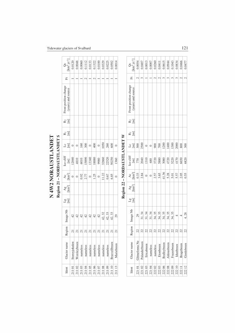
N 4
W2
NO
RA
UST
LA
ND
ET
Reg
ion
21 –
NO
RD
AU
STL
AN
DE
T S
Iden
tG
laci
er n
ame
Reg
ion
Imag
e N
bL
g[m
]A
g[k
m2 ]
Ac
[km
2 ]Ic
e−cl
iff
[m]
Lc
[m]
R1
[m]
R2
[m]
Fron
t pos
ition
cha
nge
(yea
rs)
and
sour
ceFt
Qc
[km
3yr
−1]
211
01St
oroy
joku
len
2142
012
040
01
0.01
2021
1 02
Wor
sley
bree
n21
420
4810
01
0.00
4821
1 03
nam
eles
s21
420.
9260
1016
01
0.00
6021
1 04
nam
eles
s21
422.
7715
890
300
20.
1112
211
05na
mel
ess
2142
013
340
01
0.01
3321
1 06
nam
eles
s21
421.
2518
880
400
20.
1322
211
07na
mel
ess
2142
099
800
10.
0100
211
08na
mel
ess
2142
, 32
11.2
232
860
1050
10.
0329
211
09na
mel
ess
2142
, 33
0.67
2252
026
01
0.02
2521
1 10
Bra
svel
lbre
en21
42, 3
36.
8550
250
600
10.
0502
211
13M
arie
bree
n21
290
1360
01
0.00
14
Reg
ion
22 –
NO
RD
AU
STL
AN
DE
T W
Iden
tG
laci
er n
ame
Reg
ion
Imag
e N
bL
g[m
]A
g[k
m2 ]
Ac
[km
2 ]Ic
e−cl
iff
[m]
Lc
[m]
R1
[m]
R2
[m]
Fron
t pos
ition
cha
nge
(yea
rs)
and
sour
ceFt
Qc
[km
3yr
−1]
221
01G
litne
fonn
a N
e22
290.
3377
050
02
0.00
5422
1 02
Pala
nder
bree
n22
31, 3
42.
8420
4025
003
0.04
0722
1 03
Eri
cabr
een
2231
, 34
013
100
10.
0013
221
04na
mel
ess
2231
, 34
068
00
10.
0007
222
02na
mel
ess
2234
, 35
2.57
3720
900
20.
0260
222
03E
tonb
reen
2234
, 35
3.65
5880
700
20.
0411
222
06B
odle
ybre
en22
34, 3
541
.36
3080
1200
30.
0615
222
08A
ldou
sbre
en22
34, 3
55.
2847
2014
003
0.09
4422
2 09
Fraz
erbr
een
2234
, 35
5.01
5220
1300
30.
1043
222
10Id
unbr
een
224
5.57
4170
2000
30.
0834
222
11B
rage
bree
n22
42.
0566
5080
02
0.04
6622
2 12
Gim
lebr
een
224,
28
0.55
6820
300
20.
0477
Tidewater glaciers of Svalbard 121

Reg
ion
23 –
NO
RD
AU
STL
AN
DE
T N
W
Iden
tG
laci
er n
ame
Reg
ion
Imag
eN
bL
g[m
]A
g[k
m2 ]
Ac
[km
2 ]Ic
e−cl
iff
[m]
Lc
[m]
R1
[m]
R2
[m]
Fron
t pos
ition
cha
nge
(yea
rs)
and
sour
ceFt
Qc
[km
3yr
−1]
232
03S
Fran
klin
bree
n23
2714
.29
5330
5300
30.
1065
232
04N
Fra
nklin
bree
n23
271.
0115
9080
02
0.01
11
Reg
ion
24 –
NO
RD
AU
STL
AN
DE
T N
Iden
tG
laci
er n
ame
Reg
ion
Imag
eN
bL
g[m
]A
g[k
m2 ]
Ac
[km
2 ]Ic
e−cl
iff
[m]
Lc
[m]
R1
[m]
R2
[m]
Fron
t pos
ition
cha
nge
(yea
rs)
and
sour
ceFt
Qc
[km
3yr
−1]
241
03Sa
bine
bree
n24
420
3540
01
0.00
35
242
01R
ijpbr
een
2431
, 42
8.16
2960
5600
20.
0207
Reg
ion
25 –
NO
RD
AU
STL
AN
DE
T N
E
Iden
tG
laci
er n
ame
Reg
ion
Imag
eN
bL
g[m
]A
g[k
m2 ]
Ac
[km
2 ]Ic
e−cl
iff
[m]
Lc
[m]
R1
[m]
R2
[m]
Fron
t pos
ition
cha
nge
(yea
rs)
and
sour
ceFt
Qc
[km
3yr
−1]
251
05na
mel
ess
2536
1.44
1400
1000
30.
0280
251
06D
uveb
reen
2536
1.13
1900
1000
30.
0380
252
01Sc
hwei
gaar
denb
reen
2536
, 42
3.33
5250
2000
30.
1049
252
02N
ilsen
bree
n25
360.
2034
7050
02
0.02
43
252
04L
eigh
bree
n25
425.
7225
880
600
20.
1812
122 Małgorzata Błaszczyk, Jacek A. Jania and Jon Ove Hagen

N 4
W3
SVA
LB
AR
D S
E
Reg
ion
31 –
EG
DE
ØY
A
Iden
tG
laci
er n
ame
Reg
ion
Imag
e N
bL
g[m
]A
g[k
m2 ]
Ac
[km
2 ]Ic
e−cl
iff
[m]
Lc
[m]
R1
[m]
R2
[m]
Fron
t pos
ition
cha
nge
(yea
rs)
and
sour
ceFt
Qc
[km
3yr
−1]
311
06D
elta
bree
n31
214
300
133.
90
5780
0−3
8A
STE
R, 2
001–
2004
10.
0058
313
18St
oneb
ren
3130
3720
063
2.1
7.17
5621
050
02
0.39
35
313
19K
ong
Joha
ns B
re31
3014
000
81.6
1.30
6720
300
20.
0471
Reg
ion
32 –
BA
RE
NT
SØ
YA
Iden
tG
laci
er n
ame
Reg
ion
Imag
e N
bL
g[m
]A
g[k
m2 ]
Ac
[km
2 ]Ic
e−cl
iff
[m]
Lc
[m]
R1
[m]
R2
[m]
Fron
t pos
ition
cha
nge
(yea
rs)
and
sour
ceFt
Qc
[km
3yr
−1]
321
01Fr
eem
anbr
een
328
1660
072
.20.
1220
6015
01
0.00
21
321
02D
uckw
itzbr
een
3225
1800
072
.60
230
01
0.00
02
322
02B
esse
lsbr
een
3225
2000
012
8.6
0.66
6460
300
10.
0065
Tidewater glaciers of Svalbard 123

124 Małgorzata Błaszczyk, Jacek A. Jania and Jon Ove Hagen
Fig. 12. Location map showing regions of Svalbard distinguished by Hagen et al. (1993) and numbersof sheets of maps where tidewater glaciers are present (Figs 13–30).
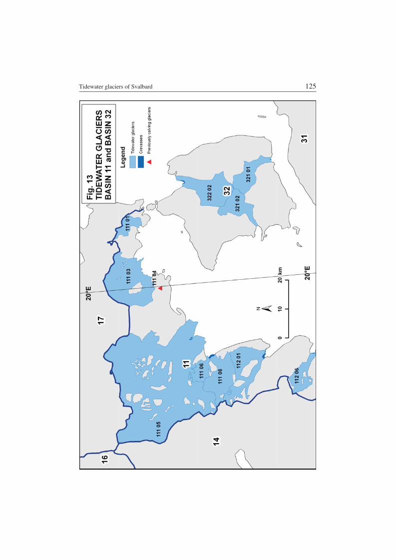
Tidewater glaciers of Svalbard 125

126 Małgorzata Błaszczyk, Jacek A. Jania and Jon Ove Hagen
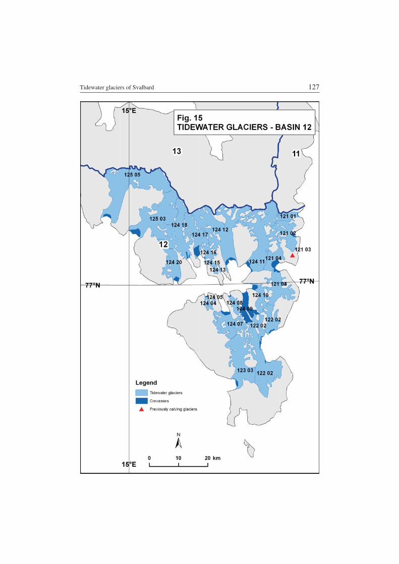
Tidewater glaciers of Svalbard 127

128 Małgorzata Błaszczyk, Jacek A. Jania and Jon Ove Hagen

Tidewater glaciers of Svalbard 129

130 Małgorzata Błaszczyk, Jacek A. Jania and Jon Ove Hagen

Tidewater glaciers of Svalbard 131

132 Małgorzata Błaszczyk, Jacek A. Jania and Jon Ove Hagen
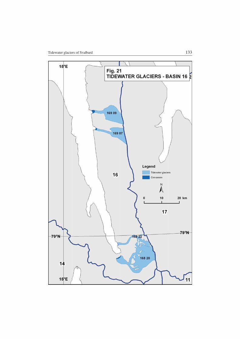
Tidewater glaciers of Svalbard 133

134 Małgorzata Błaszczyk, Jacek A. Jania and Jon Ove Hagen

Tidewater glaciers of Svalbard 135

136 Małgorzata Błaszczyk, Jacek A. Jania and Jon Ove Hagen

Tidewater glaciers of Svalbard 137
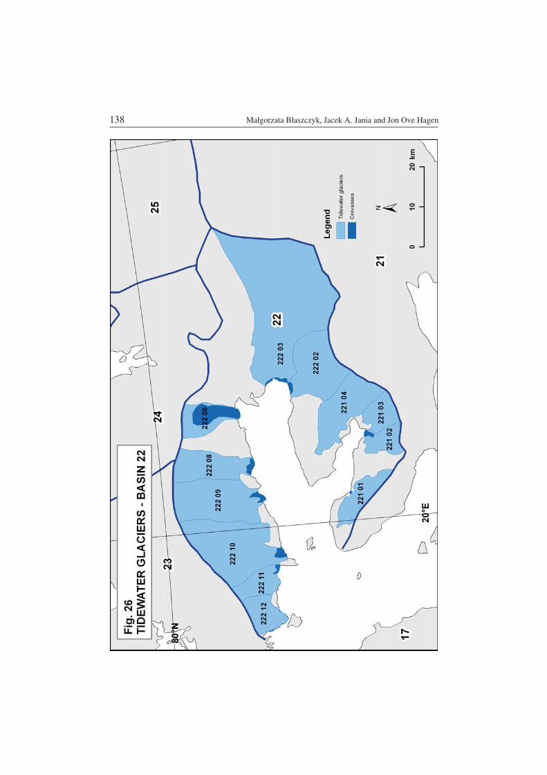
138 Małgorzata Błaszczyk, Jacek A. Jania and Jon Ove Hagen
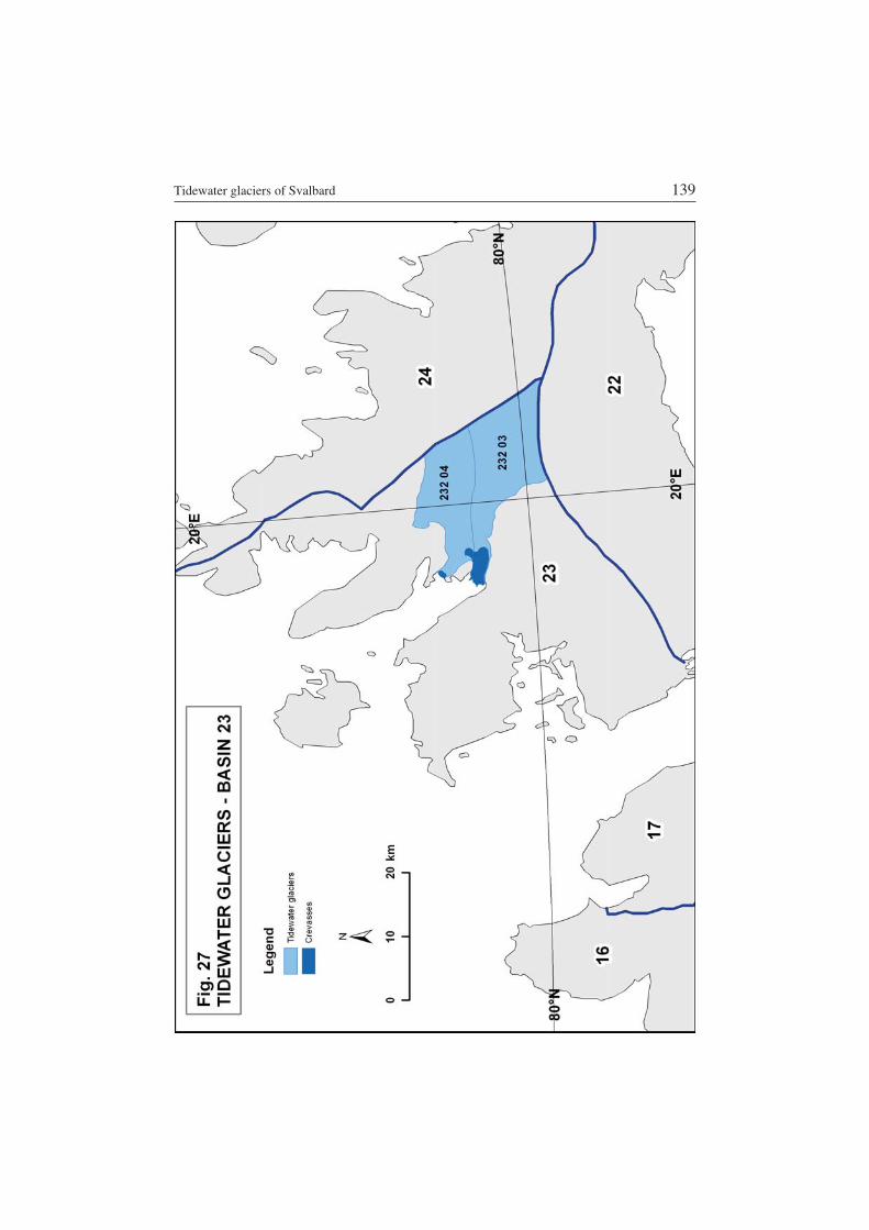
Tidewater glaciers of Svalbard 139

140 Małgorzata Błaszczyk, Jacek A. Jania and Jon Ove Hagen
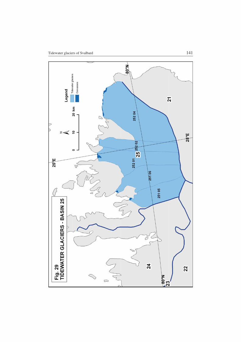
Tidewater glaciers of Svalbard 141

142 Małgorzata Błaszczyk, Jacek A. Jania and Jon Ove Hagen