
SURVEY SAMPLING IN ECONOMIC AND SOCIAL RESEARCH · Lorenzo Fattorini, Mario Glowik, Miloš Král,...
106
SURVEY SAMPLING IN ECONOMIC AND SOCIAL RESEARCH
Transcript of SURVEY SAMPLING IN ECONOMIC AND SOCIAL RESEARCH · Lorenzo Fattorini, Mario Glowik, Miloš Král,...

SURVEY SAMPLING IN ECONOMIC AND SOCIAL RESEARCH

„Studia Ekonomiczne”
ZESZYTY NAUKOWE WYDZIAŁOWE
UNIWERSYTETU EKONOMICZNEGO
W KATOWICACH
SURVEY SAMPLING IN ECONOMIC AND SOCIAL RESEARCH
Edited by
Janusz L. Wywiał and Tomasz Żądło
Katowice 2012

Komitet Redakcyjny Krystyna Lisiecka (przewodnicząca), Anna Lebda-Wyborna (sekretarz),
Florian Kuźnik, Maria Michałowska, Antoni Niederliński, Irena Pyka, Stanisław Swadźba, Tadeusz Trzaskalik, Janusz Wywiał, Teresa Żabińska
Komitet Redakcyjny Wydziału Zarządzania Janusz Wywiał (redaktor naczelny), Wojciech Gamrot (sekretarz),
Teresa Żabińska, Jacek Szołtysek, Włodzimierz Rudny
Rada Programowa Lorenzo Fattorini, Mario Glowik, Miloš Král, Bronisław Micherda,
Zdeněk Mikoláš, Marian Noga, Gwo-Hsiu Tzeng
Redaktor Elżbieta Spadzińska-Żak
© Copyright by Wydawnictwo Uniwersytetu Ekonomicznego w Katowicach 2012
ISBN 978-83-7875-040-6 ISSN 2083-8611
Wersją pierwotną „Studiów Ekonomicznych” jest wersja papierowa
Wszelkie prawa zastrzeżone. Każda reprodukcja lub adaptacja całości bądź części niniejszej publikacji, niezależnie od zastosowanej
techniki reprodukcji, wymaga pisemnej zgody Wydawcy
WYDAWNICTWO UNIWERSYTETU EKONOMICZNEGO W KATOWICACH ul. 1 Maja 50, 40-287 Katowice, tel. 32 257-76-30, fax 32 257-76-43
www.wydawnictwo.ue.katowice.pl, e-mail: [email protected]

CONTENT
INTRODUCTION ............................................................................... 7 Czesław Domański FIRST ASSOCIATIONS OF POLISH STATISTICIANS ................................ 11 Streszczenie ........................................................................................ 17 Wojciech Gamrot ON POOL-ADJACENT-VIOLATORS ALGORITHM AND ITS PERFORMANCE FOR NON-INDEPENDENT VARIABLES.................................................... 18 Streszczenie ........................................................................................ 29 Anna Imiołek, Janusz Gołaszewski, Dariusz Załuski, Zbigniew Nasalski PRACTICAL STATISTICAL AND ECONOMIC ASPECTS OF USING SURVEY STUDIES FOR IDENTIFICATION OF THE KEY PLANT CULTIVATION TECHNOLOGY FACTORS ...................................................................... 31 Streszczenie ........................................................................................ 44 Arkadiusz Kozłowski THE USEFULNESS OF PAST DATA IN SAMPLING DESIGN FOR EXIT POLL SURVEYS..................................................................... 45 Streszczenie ........................................................................................ 57 Jan Kubacki, Alina Jędrzejczak THE COMPARISON OF GENERALIZED VARIANCE FUNCTION WITH OTHER METHODS OF PRECISION ESTIMATION FOR POLISH HOUSEHOLD BUDGET SURVEY ............................................................. 58 Streszczenie ........................................................................................ 68 Dorota Raczkiewicz SOME ASPECTS OF POST ENUMERATION SURVEYS IN POPULATION CENSUSES IN POLAND AND GERMANY.................................................. 70 Streszczenie ........................................................................................ 76

Ondřej Vilikus OPTIMIZATION OF SAMPLE SIZE AND NUMBER OF TASKS PER RESPONDENT IN CONJOINT STUDIES USING SIMULATED DATASETS ..... 77 Streszczenie ........................................................................................ 83 Janusz L. Wywiał ON LIMIT DISTRIBUTION OF HORVITZ-THOMPSON STATISTIC UNDER THE REJECTIVE SAMPLING .................................................................. 84 Streszczenie ........................................................................................ 96 Tomasz Żądło ON ACCURACY OF TWO PREDICTORS FOR SPATIALLY AND TEMPORALLY CORRELATED LONGITUDINAL DATA ......................... 97 Streszczenie ........................................................................................ 105 AUTHORS ......................................................................................... 106

INTRODUCTION
Sample surveys provide one of the most challenging fields for applying the statistical methodology. They confront the researcher with a vast diversity of unique practical problems encountered in the course of studying populations. They include, but are not limited to: non-sampling errors, specific population structures, contaminated distributions of study variables, non-satisfactory sample sizes, incorporation of the auxiliary information available on many levels, simultaneous estimation of characteristics in various subpopulations, integration of data from many waves or phases of the survey and incompletely specified sampling procedures. Omnipresent constraints on time and cost additionally complicate the process of designing a survey. Dealing with such conditions brings about the need for formulating sophisticated statistical procedures dedicated to specific conditions of a sample survey. It gives birth to wide variety of approaches, methodologies and procedures borrowing the strength from virtually all branches of statistics.
This monograph was prepared on the basis of the papers that were presented during the seventh conference “Survey Sampling in Economic and Social Research” that took place on 18-20 September 2011 in Katowice, Poland. The chapters are extended and improved versions of the conference papers. Their authors deal with various theoretical and practical issues. The common motive of all papers is their relation to sample surveys.
The paper of Czesław Domański is devoted to the first three most valuable achievements of Polish statisticians and their influence on the development of international statistics. Firstly, the Author discusses the role of Tadeusz Pilat (1844-1923) professor of statistics and administration at the Lvov University as a co-founder of the International Statistical Institute. Secondly, the idea of the first Polish census conducted in 1789 is presented, which was devised and executed by a member of Parliament Fryderyk Józef earl Moszyński (1737- -1817). Thirdly, the establishment of the first Polish Chair of Statistics in the Warsaw School of Law and Administration is discussed, which was headed by Wawrzyniec Surowiecki (1769-1827) – professor of statistics and economics.
Wojciech Gamrot concentrates on the Pool-Adjacent-Violators algorithm sometimes abbreviated as PAVA. The original algorithm is formulated under the assumption of independence between random variables whose expectations are to be estimated. Several modifications of this procedure were developed in the literature but under independence. Hence, in this paper a simulation study is carried out to assess properties of PAVA-based ordered probability estimates under correlation.

INTRODUCTION 8
Anna Imiołek, Janusz Gołaszewski, Dariusz Załuski and Zbigniew Nasalski discuss practical statistical and economic aspects of using survey studies for identification of the key plant cultivation technology factors. They consider survey study carried out in 2008 in order to determine the key elements in a plant production technology and to calculate unit production costs of growing winter rye (Secale cereale L.) for grain. The surveys covered rye grain producers in northeastern Poland, who grow rye on an acreage of over 1 ha. The economic analysis was performed based on direct outlays on production; unit costs and direct margin were calculated and the structure of costs as well as profitability of winter rye production were determined.
Arkadiusz Kozłowski studies usefulness of past data in sampling design for exit poll surveys. The main stress is put on the use of widely available databases containing details of past elections results. By means of simulation experiments the effectiveness of technique of connecting the selection of new sample with past results (tied sample procedure) is evaluated and optimal parameters for this technique are indicated. A modification of the procedure is also proposed. The best results are obtained for stratified sampling with the use of elements of tied sample procedure. The possibilities of cost reduction of surveys without prejudice to the effectiveness by means of the right selection of solely large precincts are also indicated.
Jan Kubacki and Alina Jędrzejczak compare Generalized Variance Function with other methods of precision estimation for Polish Household Budget Survey. A starting point was the estimation of Balanced Repeated Replication variances or bootstrap variances in the situation where using BRR was not applicable. To evaluate the GVF model the hyperbolic function was used. The computation was done using WesVAR and SPSS software and some special procedures prepared for R-project environment. The assessment of estimates consistency for counties was also conducted by means of small area models.
Dorota Raczkiewicz presents some aspects of post enumeration surveys in population censuses in Poland and Germany. The Author begins with comparison of population censuses in Poland and Germany. Next attention is paid to data quality and potential errors in population censuses. Comparison is made of principles of post-enumeration surveys in censuses in Poland and Germany. What is more, international recommendation on quality assessment of population censuses according to the UN and EUROSTAT is presented.
Ondřej Vilikus dicussed optimization of sample size and number of tasks per respondent in conjoint studies using simulated datasets. The Author presents an approach based on analyzing batches of simulated datasets with given characteristics. The article includes overview of the results for choice-based conjoint studies with usual level of complexity. Search for an optimal combination

INTRODUCTION
9
of sample size and number of tasks per respondent that allows us to achieve required accuracy of our outputs with optimal cost is of main focus but sensitivity of the recommendations with respect to changes in fixed parameters of the datasets is also included.
Janusz L. Wywiał studies limit distribution of Horvitz-Thompson statistic under the rejective sampling. On the basis of the papers by Berger and Skinner (2005) and Hájek (1964) he considers the limit distribution of H-T statistic standardized by its sample variance. Moreover, the variance of the H-T estimator is considered under the assumption that the auxiliary variable value is the observation of the variable under study but with measuring error.
Tomasz Żądło compares accuracy of two predictors for spatially and temporally correlated longitudinal data based on Monte Carlo simulation study using R package. The first predictor under study is the empirical best linear unbiased predictor (EBLUP) derived for some special case of the General Linear Mixed Model where spatial and temporal correlations are taken into account. The second predictor is EBLUP derived under the assumption of lack of spatial and temporal correlation.


Czesław Domański
FIRST ASSOCIATIONS
OF POLISH STATISTICIANS
1. Initial Remarks
The year 2012 will witness the celebrations of the 100th anniversary of founding the Polish Statistical Society – the first association of statisticians in Poland. The present conference offers an excellent opportunity to present the contribution made by Polish statisticians towards an overall development of statistics as a discipline of science and didactics. The conference will also commemorate the jubilee of the Chair of Statistics which was established 60 years ago, first as a part of the Higher School of Economics, then the Academy of Economics and presently the Economic University in Katowice. It is worth presenting here three most valuable achievements of Polish statisticians and their influence on the development of international statistics, long before the Polish Statistical Society came into existence. 1. Conducting in 1789 the first-ever national census, which was devised and
executed by a member of Parliament Fryderyk Józef earl Moszyński (1737-1817).
2. Establishing in 1811 the Chair of Statistics in the Warsaw School of Law and Administration, which was headed by Wawrzyniec Surowiecki (1769-1827) – professor of statistics and economics.
3. Co-founding the International Statistical Institute by professor of statistics and administration at the Lvov University – Tadeusz Pilat (1844-1923).
4. Statistical congresses.
2. Statistical Congresses Before the International Statistical Institute was founded in 1840 it
became customary for scholars representing one branch of science to meet at congresses whose main aim was develop methods of posing and solving important problems. The first idea of statistical congresses was conceived in London in 1851 by Lambert Adolphe Jacques Quételet (1796-1874), the
Czesław Domański 12
chairman of the central Belgian Statististical Commission. The congresses were held in co-operation with the government of the respective country where the next session was scheduled. Standardizing of administrative statistics and adopting a general methodology of conducting censuses were the main problems discussed during subsequent statistical congresses. Altogether nine sessions of such congresses were convened in the following cities: Brussels (1853), Paris (1855), Vienna (1857), London (1860), Berlin (1863), Florence (1867), the Hague (1869), St. Petersburg (1872), Budapest (1876). At St. Petersburg Congress in 1872 a commission was set up in order to supervise works on the unification of the international statistics. In 1878 the commission proposed that a special international body, fostering cooperation between national statistical offices should be formed. However, the proposal was rejected by Germany and Switzerland who were of the opinion that such a body would unnecessarily interfere with the internal affairs of individual countries. As a result of this opposition congresses ceased to be convened, yet the idea of making statistics an international discipline was not abandoned. Following a series of meetings in Paris and London, a convention was held on June 24, 1885 in London, where the International Statistical Institute was brought into being. The convention, attended by 22 participants, was called session and from that time onwards all the regular meetings of members have become known as sessions of the International Statistical Institute (ISI).
Polish statisticians were among those statisticians who took an active part in founding the International Statistical Institute and were the Institute members. The most eminent representative of the Polish statistics of the time was August Cieszkowski (1814-1894). A. Cieszkowski, who attended the Statistical Congress in Paris in 1855, was the main speaker of one of the sessions of the Congress. The name of Tadeusz Zygmunt Pilat should also be brought here, as the first Polish member of the Institute among its 100 statutory representatives. Tadeusz Pilat (1844-1923) graduated from the University of Lvov and and continued his education in Berlin where he specialized in statistics under the scientific supervision of a renowned scholar dr Edmund Engel. In 1867 he earned his doctor’s degree in law on the basis of the doctoral dissertation Practice in all political and legal skills. Two years later Pilat obtained a postdoctoral degree having written the habilitation thesis entitled Ueber den Begriff des wirtschaftlichen Werthes and became a private associate professor in the Chair of Social Economics of the Lvov University. He was conferred his second postdoctoral degree in administrative law (1870) and developed further his knowledge of statistics during his studies in the Prussian Statistical Office in Berlin (1871). In 1872 Tadeusz Pilat was appointed assistant professor of University of Lvov and became the head of the Chair of Statistics

FIRST ASSOCIATIONS OF POLISH STATISTICIANS 13
and Administration, and a few years later (1878) he became a full professor. He was elected to be the dean of the Faculty of Law and Administration (four terms of office i.e. 1880/1881, 1884/1885, 1889/1890, 1900/1901), the President of the University (1886/1887), the Vice-President (1887/1888). Since 1909 he was an honorary professor. In the years 1876-1914 Pilat served several terms of office as a deputy for the Galicia Parliament. He headed the Statistical Office of the National Department in Lvov for over four decades (1874-1920), and worked as a deputy marshal of the National Department (1901-1920). In 1888 he was appointed a corresponding member of the Academy of Learning in Cracow, and since 1918 a member of the Polish Academy of Learning. He was also a member of the Board (1874-1902) and vice-president of the Galician Economic Society, a corresponding member of the Central Statistical Commission in Vienna (since 1876), and a full member of the Scientific Society in Lvov (since 1920). The extensive scientific output of the Author includes inter alia: Methods of Collecting Data for Harvest Statistics (1872), On Municipal Statistical Offices (1871), Composition of Commune Representation in Cities and Towns of Galicia (1874), Statistical Presentation of Communal Structure in Galicia and Results of Local Elections (1874), The Textbook of Statistics of Galicia (1900), and Statistics (1923). In his studies Pilat presented methodological problems, focusing on agricultural statistics. Among methods used in statistics of vegetable production he proposed estimation methods as an important source of statistical information. 3. First General Census in Poland
The beginnings of statistical activities on the Polish territories coincide
with the proceedings of the so called Four Year Parliament Session i.e. the years 1788-1792. The Parliament adopted a resolution on carrying out in 1789 the first national population census combined with smoke registration. The Census results were to help the Parliament to pass a bill on imposing a new tax, which was supposed to provide money towards expenses on permanent, one-hundred- -thousand army. The author of the statistical tables of the 1789 Census and a statistical method of the military tax calculation was a deputy Fryderyk Józef earl Moszyński (1737-1817). It is worth noting that although the population and smoke registration of 1789 was the first state census, numerous other registers, inventories and censuses appeared in Poland as early as 16th century (e.g. population census of the Cracow Diocese (1747-1749) and the Plock Diocese of the years 1773, 1776 and 1778) and they were conducted for tax, economic, military and church reasons. The numerical data contained in these registers
Czesław Domański 14
remain valuable source of statistical information for all kinds of estimations and analyses.
Moszyński pointed out that “the wealth of the state cannot be measured by the affluence of several aristocratic families and a couple of thousands of rich citizens, but it rather should be measured by settlements, the wealth of townspeople and countrymen, prosperous trade and flourishing crafts”. The statistical method of the military tax assessment proposed by Moszynski in the Parliament “was of absolutely unique character and it was used nowhere else either before or after that time”. In order to measure the value of land and property in a given poviat (district) in an objective way he proposed a statistical method based on the following data: – value of land and property in the poviat assessed on the basis of deeds of sales
for the period of last 11 years as recorded in district books; it was seen as representative enough for making calculations,
– number of smokes obtained from treasure tariffs; both alienated for the period of last 11 years and those which were not subject to purchase or sale.
The obtained information allowed the Treasure Commissions to make calculations based on the value of alienated goods, thanks to smoke numbers, and assess precisely the value of properties in a given poviat taking into account the proportion between smokes of alienated goods and the total.
Fryderyk Józef Moszyński supported the idea of the so-called „co- -equation” that is a fair fiscal system which made the gentry and the church pay taxes based on profits derived from their land and property.
As a result of Moszyński’s intensive efforts the Four Year Parliament (1788-1792) passed a legislative act of great importance and extremely interesting for the history of statistics in Poland – a constitution of 22 June, 1789 known as Smoke Inspection and Population Register which was in fact the first population census in the history of Poland. The census included the rural and the urban population and excluded the gentry and the clergy. It encompassed the following categories: sex, occupation and social status – observing the difference between sons (in two age groups – up to 15 years and above 15 years) and daughters.
The first estimations of the population number in Poland were produced by some of the above-mentioned statisticians. Józef Wybicki provided in 1777 the estimated number of population of 5 391 364 people; Aleksander Buching in 1772 gave the number of 8.5 million; Stanisław Staszic in 1785 estimated the population at the level of 6 million; Fryderyk Moszyński, after the first census of 1789 produced the number of 7 354 620 people; the figure did not include the gentry and the clergy, who were not the subject of the census, yet their number was estimated at the level of 750-800 thousand.

FIRST ASSOCIATIONS OF POLISH STATISTICIANS 15
4. First Chair of Statistics
The growth of interest in statistics in Poland was marked by the foundation of the first centre of statistical knowledge – the Chair of Statistics at the Warsaw School of Law and Administration in 1811. Heading the Chair was entrusted to a statistician and economist Wawrzyniec Surowiecki (1769-1827). After the first Chair of Statistics had been established, there was an upsurge in the interest in statistics as a separate branch of science and not as a tool to be used in administration. It is worth taking a closer look at the profile of the first Polish professor of statistics. He was born in Gniezno province in a gentry family of moderate means. Having completed his studies Surowiecki started professional career as a private tutor what helped him to get to know academic centres of Vienna and Dresden. In 1807 he became a member of the Warsaw Society of Friends of Sciences and at the time he already built his reputation as an expert in social issues. Although he only gave lectures in statistics for one year, he was engaged in educational and scientific activities for most of his life. In 1812 he was appointed as a secretary general in the Ministry of Education and resigned from pedagogical duties. In the Congress Kingdom of Poland he took the post in the Council for administrative affairs and educational funds.
The list of most important studies of W. Surowiecki is quite long and includes among others: On the fall of industry and towns in the old Poland (1810), On rivers and floating of the Grand Duchy of Warsaw (1810), On statistics of the Grand Duchy of Warsaw (1812-1813).
Surowiecki also took interest in the population problems and examined different reasons for population development. As a statistician he perceived wars, illiteracy, non-productive calamities and maladministration as factors which adversely affected population development.
Wawrzyniec Surowiecki together with Ignacy Stawiarski and Dominik Krysiński were the first Polish scholars to define the subject and tasks of statistics. I. Stawarski and D. Krysiński expressed their views at the meetings of the Warsaw Society of Friends of Sciences. The former voiced his opinions in September 1809 but his presentation was published in the Annals of the Society in 1812 while the latter presented them in April 1814. W. Surowiecki not only created a broad framework for statistics but also worked to develop this relatively new field of science by giving lectures in the Academy of Law and Administration in the academic year 1811/1812.

Czesław Domański 16
5. Final Remarks
Two sessions of the International Statistical Institute were held in Poland. In August 1929 Warsaw was the host of the 18th Session of the
International Statistical Institute. The fact that Poland was the organizer of the session expressed respect of the international statistical community for the achievements of Polish statistics. Six Polish representatives gave presentations in the course of the Session: – E. Szturm de Sztrem: Statistical method for examination of indices of
economic development; – E. Lipiński: Remarks on working methods of the Polish Institute of Economic
and Price Research; – S. Rzepkiewicz: On possibility of comparing crime statistics in different
countries; – S. Szulc: On the so-called standardization or improving coefficients; – J. Neyman: Contribution to the theory of reliability of statistical hypotheses; – J. Piekałkiewicz: Expenditure and revenue of public-legal associations. In September 1975 the 40th Session of the International Statistical Institute was organized in Warsaw. During the Session Polish statisticians presented the following papers: – W. Maciejewski, W. Welfe: Forecasting models for the national economy
planning and the relevance of the national information system; – K. Zagórski: Socio-demographic statistics in the system of central socio-
economic planning; – R. Bartoszyński: A model for risk of rabies; – T. Walczak: The role of modern statistical information system for management
and planning; – E. Krzeczkowska: An integrated system of international statistical comparisons; – J. Kudrycka: The possibilities of applying input-output relations to the
econometric macromodels. References Domański, Cz. (2011) Setna rocznica powstania Polskiego Towarzystwa
Statystycznego (100 years of the Polish Statistical Society). „Wiadomości Statystyczne” nr 9(604), wrzesień 2011, 1-10.
Domański, Cz. (2004) Jubileusz Polskiego Towarzystwa Statystycznego „Tradycje i obecne zadania statystyki w Polsce” (Jubilee of the Polish Statistical Society. Tradition and the present-day tasks of statistics in Poland), red. A. Zeliaś, Wydawnictwo AE Kraków.

FIRST ASSOCIATIONS OF POLISH STATISTICIANS 17
Kleczyński, J. (1886) Międzynarodowy Instytut Statystyczny (International Statistical Institute). „Przegląd Polski” rocznik XI, t. II, 354-371.
Łukaszewicz, J. (1995) Polska historiografia a statystyka (Polish historiography and statistics ). Biblioteka Wiadomości Statystycznych, t. 46, 58-68.
Romaniuk, K. (1975) Udział Polski w pracach Międzynarodowego Instytutu Statystycznego (Contribution of Poland to the work of the International Statistical Institute). „Wiadomości Statystyczne” nr 8.
PIERWSZE ZRZESZENIE POLSKICH STATYSTYKÓW
Streszczenie
W 2012 roku przypada 100. rocznica powstania pierwszego zrzeszenia statystyków polskich – Polskiego Towarzystwa Statystycznego. Warto na tej konferencji zaznaczyć wkład statystyków polskich w rozwój statystyki jako dyscypliny naukowej i dydaktycznej. Konferencja ta ma również charakter jubileuszowy, związany z 60-leciem Katedry Statystyki, działającej wcześniej w ramach Wyższej Szkoły Ekonomicznej, potem Akademii Ekonomicznej, a obecnie Uniwersytetu Ekonomicznego w Katowicach.
Wspomnijmy jedynie o trzech osiągnięciach polskich statystyków, które mają oddziaływanie międzynarodowe: 1. Przeprowadzenie w 1789 roku pierwszego spisu państwowego, którego
pomysłotwórcą i głównym realizatorem był poseł hr. Fryderyk Józef Moszyński (1737-1817).
2. Powołanie w 1811 roku Katedry Statystyki w Szkole Prawa i Administracji w Warszawie, której kierownictwo powierzono profesorowi statystyki i eko-nomii Wawrzyńcowi Surowieckiemu (1769-1827).
3. Współudział w tworzeniu Międzynarodowego Instytutu Statystycznego profesora statystyki i administracji Uniwersytetu Lwowskiego Tadeusza Pilata (1844-1923).

Wojciech Gamrot
ON POOL-ADJACENT-VIOLATORS ALGORITHM
AND ITS PERFORMANCE
FOR NON-INDEPENDENT VARIABLES
1. Introduction
Estimation of ordered expectations is a problem that has attracted attention of researchers for more than fifty years. This interest is reflected by a wide literature starting with papers of Ayer at al (1955), Brunk (1955) and van Eeden (1956, 1957, 1958), Katz (1963) as well as Hanson et al (1973), Sackrowitz and Strawderman (1974) and then developed among others by Sackrowitz (1982), Lee (1983), Best and Chakravarti (1990), Charras and van Eeden (1991), Qian (1992), Block et al (1994), Ahuja and Orlin (2001), Burdakov et al (2004), Jewel and Kalbfleisch (2004) and Hansohm (2007). A good summary of the state of knowledge is presented in monographs of Robertson et al. (1988) and van Eeden (2006).
Somehow, it appears that approaches of all these authors share a common feature. Namely, it is always assumed that random variables for which one desires to compute estimates satisfying ordering constraints are independent. This author is not aware of any estimation procedure that accounts for possible correlation between such variables. Hence two possible choices are: constructing a procedure dedicated to correlated data or investigating the properties of existing estimation strategies when independence assumption is dropped. In this paper the original Pool-Adjacent-Violators algorithm (PAVA) of Ayer et al (1955) is revisited and its properties in the case of non-zero correlation are assessed in a simulation study. 2. Pool-Adjacent-Violators algorithm
Let π1, π2, ... , πn be unknown probabilities satisfying a simple order:
π1 ≤ π2 ≤ ... ≤ πn (1)

ON POOL-ADJACENT-VIOLATORS ALGORITHM… 19
Let Ni independent trials be made of an event with probability πi for i = 1,...,n. Let yi denote the number of successes in the i-th trial and let
ii*i N/yp = for i = 1,...,n. The PAVA procedure computes estimates p1, ... , pn of
π1, ... ,πn satisfying (1) by iteratively grouping (merging) initial estimates *n
*1 p,...,p into blocks and averaging them within each block. The procedure
works through repeating following steps (see Härdle (1992), Ayer et al (1955) and de Leeuw et al (2009)). 1) Assign each component πi for i = 1,...,n to a separate group so initially n groups )0(
n)0(
1 G,...,G exist. Set initial estimate of mean probability in each i-th group to *
g)0(
g pp~ = for g = 1,...,n
2) While there exist some groups in the k-th step of algorithm such that associated estimates of mean probability violate the ordering constraint, find maximum-length sequence of such groups (say )()(
1)( ,...,, k
hk
gk
g GGG + ) and merge them
into a single group )k(h
)k(1g
)k(g
)1k(g G...GGG ∪∪∪= ++ while )k(
ghj)1k(
j GG −++ =
for j>g and assign a mean probability estimate ∑∑++ ∈∈
+ =)1k(
g)1k(
g Gii
Gii
)1k(g Nyp~ to the
group )1k(gG + while )k(
ghj)1k(
j p~p~ −++ = for j>g
3) When iteration stops after the last – say K-th – step (where K∈{0,1,...}), with H groups remaining assign a mean probability estimate computed for a group to each of its member components so that the final estimate for the component πi is
)k(gi p~p = for i∈Gg, g = 1,2,...,H
If y1,...,yn are independent, this procedure leads to a vector of restricted
maximum likelihood estimates for probabilities π1, π2, ... , πn. We will now abandon the independence assumption and allow for some correlation among yi’s. 3. A simple correlation model
To investigate properties of PAVA estimator in the case when variables are correlated we will assume a simple model stating that correlation coefficient between individual binary variables is the same for all pairs of subsequent variables: (y1, y2), (y2, y3), (y3, y4),...,(yk-1, yk). Hence a procedure generating binary random vectors in the form y = [y1,...,yk]’ satisfying E(y) = m and Cov(yi,yi-1) / V0.5(yi)V0.5(yi-1) = r for i = 2,...,k and some arbitrarily chosen

Wojciech Gamrot 20
m∈(0,1)k, r∈(0,1) is needed. Let a vector U = [U1,...,Uk]’ consist of independent components: Ui~Unif(0,1) and denote:
p11 = r (mi mi-1 (1-mi) (1-mi-1) )0.5 + mi mi-1 (2) p01= mi – p11 (3)
The first component of y may be generated as y1=J1(m1) and subsequent
components are obtained according to the formula:
⎪⎪⎩
⎪⎪⎨
⎧
=⎟⎟⎠
⎞⎜⎜⎝
⎛−
=⎟⎟⎠
⎞⎜⎜⎝
⎛
=
−−
−−
0yform1
pJ
1yformpJ
y
1i1i
01i
1i1i
11i
i (4)
where
⎩⎨⎧
≥<
=aUfor0aUfor1
)a(Ji
ii
(5)
for i = 1,...,k so that E(Ji(a)) = a.
Such a simple procedure yields a vector y satisfying desired constraints since:
i11i1101111i1i
011i
1i
11
1i1i
01i1i
1i
11i
1i1ii1i1iii
m)pm(ppp)m1(m1
pm
mp
)m1(m1
pJEm
mp
JE
)0yPr()0y|y(E)1yPr()1y|y(E)y(E
=−−=−=−−
+=
=−⎟⎟⎠
⎞⎜⎜⎝
⎛⎟⎟⎠
⎞⎜⎜⎝
⎛−
+⎟⎟⎠
⎞⎜⎜⎝
⎛⎟⎟⎠
⎞⎜⎜⎝
⎛=
===+===
−−
−−
−−
−−
−−−−
and
)y(V)y(rV) )m-(1 )m-(1m(mr mmp
mmmmp
mm)1y(P)1y|1y(P
mm)1y,1y(P)y(E)y(E)yy(E)y,y(Cov
i5.0
1i5.00.5
1-ii1-iii1i11
i1i1i1i
11i1i1i1ii
i1ii1ii1ii1ii1i
−−
−−−
−−−
−−−−−
==−=
=−=−====
=−===−=
The procedure depends on the ability to generate pseudo-random numbers U1,...,Uk imitating independent random variables having uniform distribution on (0,1). Many such generators are widely available including the fast implementation of Mersenne-Twister algorithm by Matsumoto and Nishimura (1998) implemented in the R package. This generator will be used in

ON POOL-ADJACENT-VIOLATORS ALGORITHM… 21
our study. Some sample output of the proposed procedure will now be presented. For m = [1/40, 2/40, 3/40,...,1] and r = 0 we got a typical realization of a binary random vector: y1=[0 0 0 0 0 1 0 0 0 1 0 0 0 0 1 1 0 0 1 1 1 1 0 1 1 1 1 0 1 0 0 1 1 1 1 1 1 1 1 1] For m = [0.5,...,0.5] and r = 0 we got a typical realization: y2=[1 0 0 1 1 0 0 1 0 1 0 0 1 0 1 0 0 0 1 0 1 1 0 0 1 1 1 0 0 0 0 1 1 0 0 0 1 1 1 1] For m = [0.5,...,0.5] and r = 0.8 we got a typical realization: y3=[1 1 1 1 1 0 0 0 0 0 0 0 0 0 0 0 0 0 0 0 0 0 0 0 0 1 1 1 1 1 1 1 1 1 1 1 1 1 1 1] For m = [0.5,...,0.5] and r = -0.8 we got a typical realization: y4 = [0 1 0 1 0 1 0 1 0 1 0 1 0 1 0 1 0 1 1 0 1 0 1 0 1 1 1 0 0 1 0 1 0 1 0 1 0 1 1 0] 4. Simulation results
A simulation study was carried out in order to assess how the bias and mean square error of PAVA estimates for ordered probabilities depend on the sample size when variables are correlated. Three simulation experiments were carried out. In each experiment the sequence of n = 20,40,...,200 binary vectors was generated independently h = 30000 times using the procedure described in previous section. All the experiments were carried out using scripts in R (R Development Core Team (2011)). PAVA estimates were computed using the ‘gpava’ function implemented in the R ‘isotone’ package (see de Leeuw et al (2009) for a description). In the first experiment marginal probabilities were set to:
m1 = [0.48, 0.49, 0.5, 0.51,0.52] with r = 0.0, 0.2, 0.5, 0.8. In the second experiment they were set to
m2 = [0.33, 0.33, 0.35, 0.37,0.37] with r = 0.0, 0.2, 0.5, 0.8. In the third experiment marginal probabilities amounted to:
m3 = m1 = [0.48, 0.49, 0.5, 0.51,0.52]

Wojciech Gamrot 22
with r = 0.0, -0.2, -0.5, -0.8. Marginal probabilities were chosen close to each other in order to make the effects of correcting breached constraints by PAVA clearly visible. The bias and mean square error observed in the first experiment are shown in figures 1 and 2. The bias and mean square error observed in the second experiment are shown in figures 3 and 4. The bias and mean square error observed in the third experiment are shown in figures 5 and 6.
50 100 150 200
-0.0
40.
000.
04
r= 0
Bia
s(...
)
50 100 150 200-0
.04
0.00
0.04
r= 0.2
Bia
s(...
)
50 100 150 200
-0.0
40.
000.
04
r= 0.5
Bia
s(...
)
50 100 150 200
-0.0
40.
000.
04
r= 0.8
Bia
s(...
)
p1p2
p3p4p5
Fig. 1. The bias of PAVA estimates for m = m1 and r = 0.0, 0.2, 0.5, 0.8
In all three experiments the scope of observed bias depends on the position of a variable in the simple order (1). The bias for estimates p4 and p5 of rightmost probabilities π4 and π5 tends to be positive while for leftmost probabilities π1 and π2 the bias of estimators p1 and p2 tends to be negative.

ON POOL-ADJACENT-VIOLATORS ALGORITHM… 23
Meanwhile, estimator p3 of the innermost probability π3 seems to be approximately unbiased. The introduction of strong positive correlation in the first and second experiment seems to reduce the bias to some extent. The effect of negative correlation assessed in the third experiment is more complex: estimates of outermost variables π1 and π5 seem to be unaffected while the bias of estimates for π2 and π4 is slightly reduced. Anyway, in all experiments and for all parameters π1,..., π5 the bias of estimates apparently tends to zero when sample size n increases. Hence there is no evidence that the asymptotic unbiasedness of PAVA estimates which was proven by Ayer et al (1955) under assumption of independence ceases to hold in the presence of correlation.
50 100 150 200
5e-0
42e
-03
1e-0
2
r= 0
MS
E(..
.)
50 100 150 200
5e-0
42e
-03
1e-0
2
r= 0.2
MS
E(..
.)p1p2p3p4p5
50 100 150 200
5e-0
42e
-03
1e-0
2
r= 0.5
MS
E(..
.)
50 100 150 200
5e-0
42e
-03
1e-0
2
r= 0.8
MS
E(..
.)
Fig. 2. The MSE of PAVA estimates for m = m1 and r = 0.0, 0.2, 0.5, 0.8

Wojciech Gamrot 24
50 100 150 200
-0.0
40.
000.
04
r= 0
Bia
s(...
)
50 100 150 200
-0.0
40.
000.
04
r= 0.2
Bia
s(...
)
50 100 150 200
-0.0
40.
000.
04
r= 0.5
Bia
s(...
)
50 100 150 200
-0.0
40.
000.
04
r= 0.8
Bia
s(...
)p1p2
p3p4p5
Fig. 3. The bias of PAVA estimates for m = m2 and r = 0.0, 0.2, 0.5, 0.8
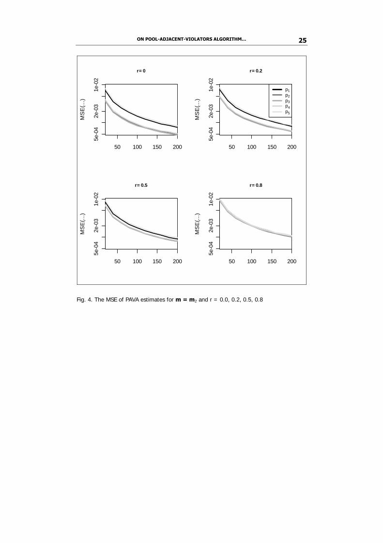
The mean square error of estimates depends on a position of a variable in the order (1) as well. In all three experiments the MSE for estimators p1 and p5 is clearly the highest of all the five and only in the second experiment the observed difference between these two is more pronounced (with p1 being somehow more accurate than p5). Anyway, in all experiments the MSE of all estimators p1,...,p5 apparently tends to zero with growing sample size which suggests that consistency is retained under correlation.
ON POOL-ADJACENT-VIOLATORS ALGORITHM… 25
50 100 150 200
5e-0
42e
-03
1e-0
2
r= 0
MS
E(..
.)
50 100 150 200
5e-0
42e
-03
1e-0
2
r= 0.2
MS
E(..
.)
p1p2p3p4p5
50 100 150 200
5e-0
42e
-03
1e-0
2
r= 0.5
MS
E(..
.)
50 100 150 200
5e-0
42e
-03
1e-0
2
r= 0.8
MS
E(..
.)
Fig. 4. The MSE of PAVA estimates for m = m2 and r = 0.0, 0.2, 0.5, 0.8
Wojciech Gamrot 26
50 100 150 200
-0.0
50.
05
r= 0
Bia
s(...
)
50 100 150 200
-0.0
50.
05
r= -0.2
Bia
s(...
)
50 100 150 200
-0.0
50.
05
r= -0.5
Bia
s(...
)
50 100 150 200
-0.0
50.
05
r= -0.8
Bia
s(...
)p1p2
p3p4p5
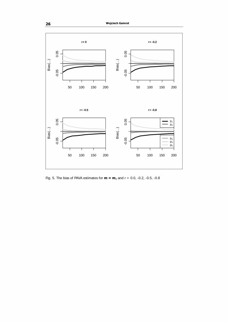
Fig. 5. The bias of PAVA estimates for m = m3 and r = 0.0, -0.2, -0.5, -0.8

ON POOL-ADJACENT-VIOLATORS ALGORITHM… 27
50 100 150 200
2e-0
42e
-03
2e-0
2
r= 0
MS
E(..
.)
50 100 150 200
2e-0
42e
-03
2e-0
2
r= -0.2
MS
E(..
.)
50 100 150 200
2e-0
42e
-03
2e-0
2
r= -0.5
MS
E(..
.)
50 100 150 200
2e-0
42e
-03
2e-0
2
r= -0.8
MS
E(..
.)p1p2p3p4p5
Fig. 6. The MSE of PAVA estimates for m = m3 and r = 0.0, -0.2, -0.5, -0.8 5. Conclusion
Simulation experiments carried out during this study covered several multivariate distributions of a binary vector y, involving dependencies between its individual components. Even for very strong correlations, no evidence of any departures from the consistency property was found. Hence, presented results suggest that PAVA estimates may retain consistency in the situation when binary variables are correlated. Obviously, those promising simulation results do not constitute a formal proof of consistency as they cover only a few of infinitely many possible combinations of parameters. However they justify theoretical efforts aimed at establishing properties of PAVA-based estimates under correlation. Such efforts may significantly widen the range of possible applications for the PAVA procedure.

Wojciech Gamrot 28
References Ahuja, R.K., Orlin, J.B. (2001) A fast scaling algorithm for minimizing
separable convex functions subject to chain constraints. “Operations Research” 49, 784-789.
Ayer, M., Brunk, H.D., Ewing, G.M., Reid, W.T., Silverman, E. (1955) An empirical Distribution function for Sampling with Incomplete Information. “The Annals of Mathematical Statistics” 6(4), 641-647.
Best, M.J., Chakravarti, N. (1990) Active Set Algorithms for Isotonic Regression; A Unifying Framework. “Mathematical Programming” 47, 425-439.
Block, H., Qian, S., Sampson, A. (1994) “Journal of Computational and Graphical Statistics” 3(3), 285-300.
Brunk, H.B., (1955) Maximum likelihood estimates of monotone parameters. “The Annals of Mathematical Statistics” 26, 607-616.
Burdakov, O., Grimwall, A., Hussian, M. (2004) A Generalized PAV Algorithm for Monotonic Regression in Several Variables. COMPSTAT Proceedings in Computational Statistics. Physica-Verlag/Springer, Heidelberg, 761-767.
Charras, A., van Eeden, C. (1991) Bayes and admissibility properties of estimators in truncated parameter spaces. “Canadian Journal of Statistics” 19, 121-134.
van Eeden, C. (1956) Maximum likelihood estimation of ordered probabilities. Proc. Kon. Nederl. Akad. Wetensch. Ser. A. 60, 128-136.
van Eeden, C. (1957) Maximum likelihood estimation of partially or completely ordered probabilities. Proc. Kon. Nederl. Akad. Wetensch. Ser. A. 59, 444-455.
van Eeden, C. (1958) Testing and estimating ordered parameters of probability distributions. Ph.D. thesis, University of Amsterdam.
van Eeden, C. (2006) Restricted Parameter Space Estimation Problems: Admissibility and Minimaxity Results. Springer. New York.
de Leeuw, J., Hornik, K., Mair, P. (2009) Isotone optimization in R: Pool-adjacent-violators algorithm (PAVA) and active set methods. “Journal of Statistical Software” 32(5), 1-24.
Hansohm, J. (2007) Algorithms and error estimations for monotone regression on partially preordered sets. “Journal of Multivariate Analysis” 98, 1043-1050.

ON POOL-ADJACENT-VIOLATORS ALGORITHM… 29
Hanson, D.L., Pledger G.., Wright F.T. (1973) On Consistency in Monotonic Regression. “The Annals of Statistics” 1(3), 401-421.
Härdle W. (1992) Applied Nonparametric Regression. Cambridge University Press.
Jewel, N.P., Kalbfleisch, J.D. (2004) Maximum likelihood estimation of ordered multinomial probabilities, “Biometrics” 5(2), 291-306.
Katz, M.W. (1963) Estimating ordered probabilities. “Annals of Mathematical Statistics” 34, 967-972.
Lee, C.C. (1983) The min-max algorithm and isotonic regression. “Annals of Statistics” 11, 467-477.
Matsumoto, M., Nishimura, T. (1998) Mersenne twister: a 623-dimensionally equidistributed uniform pseudo-random number generator. “ACM Transactions on Modeling and Computer Simulation” 8 (1), 3-30.
Qian, S. (1992) Minimum lower sets algorithm for isotonic regression. “Statistical Probability Letters” 15, 31-35.
R Development Core Team (2010) A language and environment for statistical computing. R Foundation for Statistical Computing, Vienna.
Robertson, T., Wright, F.T., Dykstra, R.L. (1988) Order restricted statistical inference. Wiley, New York.
Sackrowitz, H. (1982) Procedures for improving the MLE for ordered binomial parameters. “Journal of Statistical Planning and Inference” 6, 287-296.
Sackrowitz, H., Strawderman, W. (1974) On the admissibility of the M.L.E. for ordered binomial parameters. “Annals of Statistics” 2, 822-828.
O WŁASNOŚCIACH ALGORYTMU PAVA DLA ZMIENNYCH ZALEŻNYCH
Streszczenie
Algorytm PAVA (od ang. Pool-Adjacent-Violators Algorithm) jest po-pularnym narzędziem estymacji wykorzystywanym do szacowania wartości oczekiwanych ciągu zmiennych losowych w sytuacji, gdy dostępna informacja dodatkowa pozwala stwierdzić, że między tymi wartościami oczekiwanymi zachodzi relacja porządku. Uzyskane za pomocą tego algorytmu oszacowania maksymalizują (warunkowo) funkcję wiarogodności przy założeniu, że relacja ta

Wojciech Gamrot 30
jest spełniona oraz poszczególne zmienne są niezależne. Wydaje się, że żadna z przedstawionych w literaturze przedmiotu modyfikacji tej procedury estymacji nie uwzględnia możliwości wystąpienia zależności pomiędzy poszczególnym zmiennymi. W niniejszym artykule przedstawiono rezultaty eksperymentów symulacyjnych których celem było zbadanie własności oszacowań uzyskanych za pomocą tej procedury gdy zmienne są skorelowane.

Anna Imiołek Janusz Gołaszewski Dariusz Załuski Zbigniew Nasalski
PRACTICAL STATISTICAL AND ECONOMIC
ASPECTS OF USING SURVEY STUDIES
FOR IDENTIFICATION OF THE KEY PLANT
CULTIVATION TECHNOLOGY FACTORS
1. Introduction Survey studies are a research method that is widespread in social sciences
but less common in agro-technical studies. Among the publications which have appeared in Poland, mainly concerned with the methodology of using surveys for evaluation of plant cultivation technologies and agro-technical factors, noteworthy are papers written by Krzymuski (1982), Krzymuski et al.(1995), Laudański et al. (2007a, 2007b) and Imiołek et al. (2010).
Plant production is governed by certain, well-defined cultivation recommendations, especially important when quality standards imposed by contract agreements are to be met. Due to technical and economic conditions, a farmer is not always able to adhere to such recommendations in practice, but at the same time changes on the farm produce market enforce producers to either change or modify a production technology. Selecting an adequate combination of agro-technical factors depends on the qualitative and quantitative parameters of a market product (yield), but the decision is also shaped by such organization of plant production which enables the farmer to minimize production costs and maximize the profit. The volume and quality of yield are a product of many factors, which comprise elements of plant agro-technology and random events. A general problem in all research methods is the identification of factors which can be named as the key ones in a given technology. In the present study, it has been assumed that creating a new cultivation technology or modifying an existing begin through the recognition of the technological foundations of

Anna Imiołek, Janusz Gołaszewski, Dariusz Załuski, Zbigniew Nasalski 32
production. In respect of the methodology, a decision to use surveys has been made.
Because the research covered a large area, it was rather difficult to have the survey completed by all agricultural producers. Survey studies are significantly affected by the time which elapses from events which a survey investigates to the time when respondents are interviewed and the form of questions (Conrad et al. 2009). Winter crops cultivation is characterized by relatively long duration. For the respondents’ replies to be reliable, a survey should be completed as soon as possible after the termination of a production process and before a new cycle begins. Another difficulty in survey-based studies is the general unwillingness of agricultural producers to reveal detailed information about the agro-technical factors of the production they conduct (except situations when monitoring production on a given farm is compulsory). Therefore, the results of surveys, even when applied to a representative sample, can be burdened with an error and although they are a valuable material for scientific research, they should not be used for making production recommendations. When planning this survey study, the authors presumed that it should generate a general view of the configuration of factors involved in rye cultivation technology and enable economic evaluation of the production as well as selection of factors for further examination in strict experiments.
This paper is therefore an attempt at using survey data for evaluation of a technology of rye cultivation, making an economic evaluation and selecting key agro-technical factors. 2. Methodology of survey studies
The present survey on the technology of growing winter rye covered the area of northeastern Poland, the provinces of Warmia and Mazury, Podlasie and Mazowsze. In order to reflect the current economic status of agricultural producers, our selection of respondents was intentional and the size of a winter rye plantation over 1 ha was the selection criterion. Most of the surveyed farms grew rye under contracts with rye processing plants (mainly mills). During direct interviews at farms, survey questionnaires were completed. The questionnaire was divided into four groups of questions, which were to determine the value of a plantation, pre-sowing treatments, quality of seed material, agro-technical aspects of grain sowing, plantation treatments and harvest.
Statistical analysis of the surveys. The preliminary stage of statistical analysis of the data provided by the questionnaires consisted of coding the data. The factors were divided into natural categories (e.g. forecrops) or class ranges (e.g. levels of nitrogen fertilization) according to the technological guidelines for rye cultivation given in the references.

PRACTICAL STATISTICAL AND ECONOMIC ASPECTS OF USING SURVEY STUDIES… 33
The next step in our analysis consisted of creating a linear model and analyzing grain yields per ha for the whole sample population and divided into biological forms of cultivars, i.e. hybrid and population. For the particular types of cultivars, the model included only such agro-technical factors that were involved in a technology of growing those cultivars.
For assessment of the main effects of the factors and de-composition of the contribution of particular production factors into the variability of grain yield, type III sums of squares were used and the coefficient 2η (eta-square) was determined, which reflected the relative contribution of an examined production factor to the volume of yield.
..2 / OgEf SSSS=η
where: .EfSS is the sum of squares of the variability of a given effect, and .OgSS is the sum of squares of the general variability of a model.
In the later part of statistical analysis, a hierarchy of the cultivation
technology factors was established (evaluation of the importance of factors) via an application of classification trees – analyses were made for the whole population and divided into cultivar forms. The classification trees were constructed from a learning set, which consisted of the upper and lower quartile of the population, corresponding, respectively, to low and high yields. The C&RT (Classification and Regression Trees) method was applied to constructing a tree that exhausted the search for one-dimensional divisions. This method verifies all possible divisions for each predictive variable in order to find out a division for which the best improvement of the goodness of fit (or else the highest reduction in the lack of fit) appears. The goodness of fit was determined with the Gini coefficient, which reaches the value 0 when only one class appears in a given node. For stopping the division, the option ‘cut at an error of wrong classification’ was chosen, so that a tree was divided until the moment when all the nodes were clear (containing objects from only one class) or having no more than a specified maximum number of objects. This number was set as 5. The size of a tree was set according to V-fold cross-validation. All statistical analyses were performed with the aid of the computer software STATISTICA ® 9.0.
The economic analysis of the results. The inventory of treatments and applied equipment was used for determination of labour, tractive power and technological devices as well as material outlays used for cultivation of rye. The costs of exploitation of technical means were computed with the method suggested by the Institute of Economics and Agricultural machinery Exploitation, the Institute of Civil Engineering and Agricultural Machinery in Warsaw (Muzalewski 2010). The material costs (e.g. mineral fertilizers, plant

Anna Imiołek, Janusz Gołaszewski, Dariusz Załuski, Zbigniew Nasalski 34
protection chemicals) were determined as a product of their use and price per unit. For the calculations, the market prices as of June 2010 were taken. The parity rate per 1 hour of labour was computed according to the average pay in the whole Polish economy (www.stat.gov.pl.), assuming that – as the EUROSTAT claims – 1 person can work no more than 1 annual work unit (AWU), even if they actually work longer. The annual work unit (AWU) is an equivalent of the time taken to perform the work done by 1 person employed on a full-time basis at a farm. In Poland, it is assumed that 2,120 hours of work per year are an equivalent of a full-time job in agriculture (www.stat.gov.pl.). The value of outlays originating from own production (seed material) was estimated with the own costs method. The cost of mineral fertilizers was assessed by the comparative method, transferring the average market value of the fertilizer’s mineral components onto the analogous components found in FYM, taking into consideration the amount of nitrogen applicable in a given year. The direct costs also include the surcharge of indirect costs. The production profitability index, understood as a ratio of the value of production which is a potential commodity to the total costs of the production outlays, was applied as a synthetic economic measure which regarded the effectiveness of the outlays (Nasalski et al. 2004).
The costs have been presented in a functional pattern, distinguishing particular outlays related with a given treatment, i.e. pre-sowing soil tillage, sowing, fertilization, application of plant protection chemicals. The costs of the treatments include the outlays on exploitation of machines, labour outlays and expenditures on material production means.
3. The results
The survey study encompassed 73 villages in ten administrative districts
lying in three province: Warmia and Mazury, Podlasie and Mazowsze. During face-to-face interviews, 201 questionnaires were filled in; they covered environmentally different variants of rye production on 153 farms, which had at least 1 ha of winter rye grown for grain in their structure of crops sown in 2007/2008.
When the data from all the plantations were collected, the analysis of variance of the rye grain yields demonstrated the significance of all the main effects, except pre-sowing tillage and pre-sowing fertilization. In turn, the analysis of the production technology applied to hybrid cultivars proved that the pre-sowing tillage, seed dressing and weed and fungus control treatments were non-significant, but when population rye was grown, the non-significant factors included pre-sowing tillage, seed certification grade, sowing technique, row spacing, fungal control and application of a retardant.

PRACTICAL STATISTICAL AND ECONOMIC ASPECTS OF USING SURVEY STUDIES… 35
Fig. 1. The area covered by the surveys and number of surveys in the administrative districts of northeastern Poland
Table 1 Analysis of variance of grain yield of rye
Hybrid cultivars Population cultivars Specification
df SS III p df SS III p
Organic fertilization 1 17.09 0.00 1 4.56 0.00
Pre-sowing cultivation 1 0.01 0.70 1 0.61 0.22
Pre-sowing fertilization 1 1.55 0.00 2 21.39 0.00
Cultivars 3a 20.28 0.00 5a 64.21 0.00
Seed certification 2 0.94 0.00 3 2.55 0.10
Seed dressing 1 0.08 0.30 1 7.83 0.00
Sowing technique 1 0.34 0.03 1 0.00 0.95
Date of sowing 2 0.54 0.02 2 3.73 0.01
Sowing rate 2 9.03 0.00 1 17.83 0.00
Row spacing 1 0.87 0.00 1 0.13 0.57
Depth of sowing 2 30.01 0.00 4 12.57 0.00

Anna Imiołek, Janusz Gołaszewski, Dariusz Załuski, Zbigniew Nasalski 36
Top dressing 1 0.67 0.00 2 49.77 0.00
Mechanical cultivationb 1 6.28 0.00
Fungicide application 1 0.24 0.07 1 0.41 0.31
Herbicide application 1 0.09 0.73 1 14.18 0.00
Retardant application 1 2.41 0.00 1 0.26 0.42
Date of harvest 2 10.04 0.00 3 10.18 0.00
Error 832 60.11 951 384.08
In total 855 482.96 982 711.79
a when analyzed cultivars were a factor tested by the analysis covering types of cultivars
b the factor was absent from the technology
The de-composition of contribution of particular production factors to the total variability demonstrated that the random factors made up the largest contribution to the variability of rye grain yields, especially in the case of hybrid rye (61%) (fig. 2). The major factors determining the yield of rye grains were the date and parameters of sowing. In respect of the type of cultivars, large differentiation was discovered. When growing population cultivars, the factors related to seed quality and plant cultivation treatments were found to dominate, whereas in the cultivation of hybrid varieties, where the seed material is exchanged on 66% of the analyzed plantations, the dominant effect was produced by the agro-technical factors connected with seed sowing.
Fig. 2. Decomposition of variability of factors in winter rye production

PRACTICAL STATISTICAL AND ECONOMIC ASPECTS OF USING SURVEY STUDIES… 37
Depending on the form of rye, the volume of average grain yields varied by 1.05 t. Three classification trees were constructed for the total rye population and for the two rye forms: population and hybrid varieties. On each occasion, the learning set consisted of the upper and lower quartile of yields. The major factor discriminating rye production (based on the results from all the rye plantations) was the sowing rate. High yields classified initially as low ones were discriminated by the soil class and soil complex, as well as nitrogen dressing. For the population cultivars, the moment the cultivation technology factors had been included, the major determinant was the application of seed dressing (fig. 3). High yields initially classified as low ones were determined by nitrogen top dressing, followed by the date of sowing, row spacing and plant protection measures such as the application of a herbicide.
Fig. 3. Classification tree of low and high yields of winter rye population cultivars
In respect of hybrid forms, high yields were obtainable at a low sowing rate (in accord with the cultivation recommendations prepared for hybrid rye) and application of a herbicide (fig. 4). High yields initially classified as low ones were determined by the parameters defining the quality of sowing seeds and the date of sowing.
Fig. 4. Classification tree of low and high yields of winter rye hybrid cultivars

Anna Imiołek, Janusz Gołaszewski, Dariusz Załuski, Zbigniew Nasalski 38
Among the analyzed production factors, ranks achieved for hybrid varieties were much different from the ones for population forms (fig. 5). The highest ranks were achieved by the parameters related to sowing, row spacing 79% for pre-sowing tillage and 76% for the sowing rate. In contrast, for population cultivars the highest rank was scored by weed control measures, followed by parameters connected with the quality of seed material, cultivars and nitrogen top dressing.
Fig. 5. Ranking of the importance of some variables for population and hybrid cultivars [%]
The costs calculation in agricultural practice should be used as a source of
information useful when making strategic decisions as well as operational ones. Economic analysis enables farmers to optimize the production structure and to make a more rational use of particular techniques. When cereal prices are unstable, one of the very few chances to improve the economic output on farms which grow cereals as a commodity is the verification of outlays and costs (Nasalski et al. 2004).
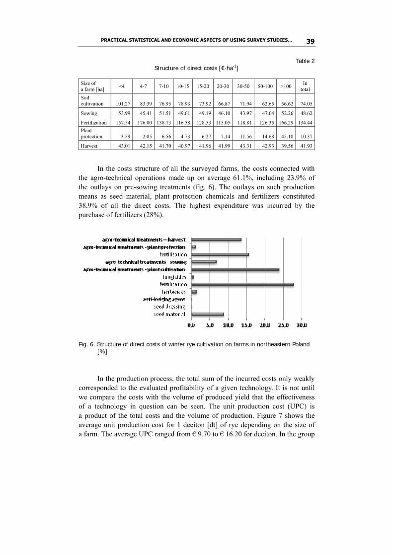
The volume and quality of rye grain yield were significantly shaped by fertilization. As demonstrated by the conducted survey, 40% of the total direct costs were incurred by fertilization operations alongside the expenditure on the purchase of fertilizers (table 2). The costs related to chemical protection of rye plants were extremely varied, depending on the size of a farm. On farms which had up to 7 ha of arable land, they hardly reached 1%, but went up to 12% on farms which had over 100 ha of acreage. The outlays on soil tillage before sowing were lower in larger farms, which possess more efficient machines and can aggregate the performed operations.
PRACTICAL STATISTICAL AND ECONOMIC ASPECTS OF USING SURVEY STUDIES… 39
Table 2 Structure of direct costs [€·ha-1]
Size of a farm [ha] <4 4-7 7-10 10-15 15-20 20-30 30-50 50-100 >100 In
total Soil cultivation 101.27 83.39 76.95 78.93 73.92 66.87 71.94 62.65 56.62 74.05
Sowing 53.99 45.41 51.51 49.61 49.19 46.10 43.97 47.64 52.26 48.62
Fertilization 157.54 176.00 138.73 116.58 128.53 115.05 118.81 126.35 166.29 134.44 Plant protection 3.59 2.05 6.56 4.73 6.27 7.14 11.56 14.68 45.10 10.37
Harvest 43.01 42.15 41.70 40.97 41.96 41.99 43.31 42.93 39.56 41.93
In the costs structure of all the surveyed farms, the costs connected with the agro-technical operations made up on average 61.1%, including 23.9% of the outlays on pre-sowing treatments (fig. 6). The outlays on such production means as seed material, plant protection chemicals and fertilizers constituted 38.9% of all the direct costs. The highest expenditure was incurred by the purchase of fertilizers (28%).
Fig. 6. Structure of direct costs of winter rye cultivation on farms in northeastern Poland
[%] In the production process, the total sum of the incurred costs only weakly
corresponded to the evaluated profitability of a given technology. It is not until we compare the costs with the volume of produced yield that the effectiveness of a technology in question can be seen. The unit production cost (UPC) is a product of the total costs and the volume of production. Figure 7 shows the average unit production cost for 1 deciton [dt] of rye depending on the size of a farm. The average UPC ranged from € 9.70 to € 16.20 for deciton. In the group
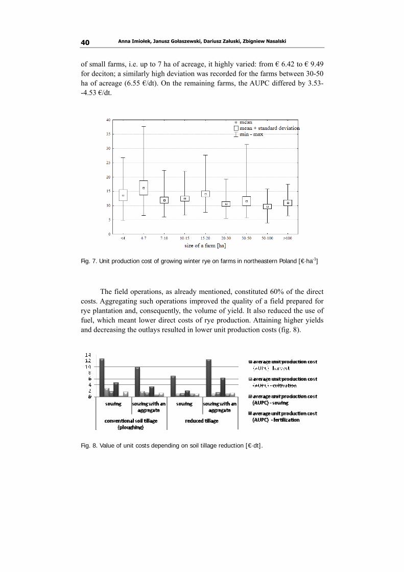
Anna Imiołek, Janusz Gołaszewski, Dariusz Załuski, Zbigniew Nasalski 40
of small farms, i.e. up to 7 ha of acreage, it highly varied: from € 6.42 to € 9.49 for deciton; a similarly high deviation was recorded for the farms between 30-50 ha of acreage (6.55 €/dt). On the remaining farms, the AUPC differed by 3.53- -4.53 €/dt.
Fig. 7. Unit production cost of growing winter rye on farms in northeastern Poland [€·ha-1]
The field operations, as already mentioned, constituted 60% of the direct costs. Aggregating such operations improved the quality of a field prepared for rye plantation and, consequently, the volume of yield. It also reduced the use of fuel, which meant lower direct costs of rye production. Attaining higher yields and decreasing the outlays resulted in lower unit production costs (fig. 8).
Fig. 8. Value of unit costs depending on soil tillage reduction [€·dt].
PRACTICAL STATISTICAL AND ECONOMIC ASPECTS OF USING SURVEY STUDIES… 41
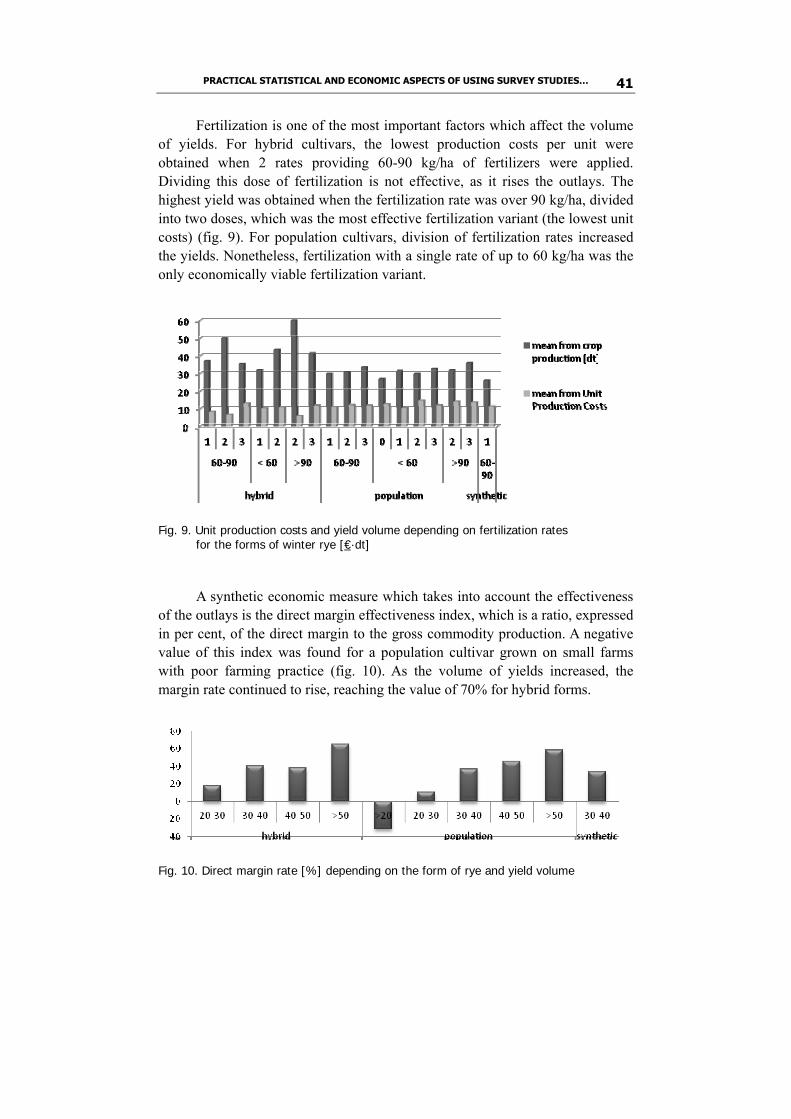
Fertilization is one of the most important factors which affect the volume of yields. For hybrid cultivars, the lowest production costs per unit were obtained when 2 rates providing 60-90 kg/ha of fertilizers were applied. Dividing this dose of fertilization is not effective, as it rises the outlays. The highest yield was obtained when the fertilization rate was over 90 kg/ha, divided into two doses, which was the most effective fertilization variant (the lowest unit costs) (fig. 9). For population cultivars, division of fertilization rates increased the yields. Nonetheless, fertilization with a single rate of up to 60 kg/ha was the only economically viable fertilization variant.
Fig. 9. Unit production costs and yield volume depending on fertilization rates
for the forms of winter rye [€·dt]
A synthetic economic measure which takes into account the effectiveness of the outlays is the direct margin effectiveness index, which is a ratio, expressed in per cent, of the direct margin to the gross commodity production. A negative value of this index was found for a population cultivar grown on small farms with poor farming practice (fig. 10). As the volume of yields increased, the margin rate continued to rise, reaching the value of 70% for hybrid forms.
Fig. 10. Direct margin rate [%] depending on the form of rye and yield volume

Anna Imiołek, Janusz Gołaszewski, Dariusz Załuski, Zbigniew Nasalski 42
Production operations are under the influence of some endogenous factors: the production potential of each farm, i.e. land, labour and capital resources, their quality and usability, and exogenous ones, produced by some external influence produced on agriculture (Skarżyńska 2010). Market prices for rye are highly unstable, varying from year to year between 80.5 and 20.12 euro per dt-1 (www.minrol.gov.pl/pol/Rynki-rolne). Beside the indirect income obtained from selling grain, farmers also receive subsidies, which largely affect the profit obtained from this type of production, especially on small, low- -productivity farms, which would generate loss was it not for the subsidies they are paid (fig. 11). Low yields obtained on organic farms are compensated for only by higher subsidies.
Fig. 11. Profit obtained from rye production depending on a) rye form and yield volume
[€·ha-1], b) type of farm management
4. Conclusions
A survey study, carried out in the form of face-to-face interviews, can be a source of valuable data on the currently applied plant production technologies over an area covered by that research, and the ANOVA methods, including type III sums of squares and classification trees, can properly discriminate among the analyzed factors, allowing researchers to identify the key factors necessary to obtain high yields.
When different types of agricultural cultivars are grown, the results of surveys and of the subsequent analyses will enable us to capture these production factors which are universal in character and the ones which are specific for a given type of crops.
In rye cultivation, 39% of the grain yield variability is attributable to the quality of a cultivation field. The production techniques significantly differentiate
PRACTICAL STATISTICAL AND ECONOMIC ASPECTS OF USING SURVEY STUDIES… 43
between the types of rye – hybrid and population varieties. Better yielding hybrid cultivars are highly variable in terms of the factors connected with the quality of seed material and plant cultivation treatments, whereas the group of most significant agro-technical factors in cultivation of population cultivars comprises the seed sowing techniques. It is among these groups of rye grain production factors that we should identify the ones for testing in strict and production experiments.
The economic analysis of the results of our survey shows what costs rye cultivation incurs, which can change due to growing prices of different raw materials but which are also dependent on the applied technology, cultivation acreage, labour potential or the available machines and tools.
The economic costs calculation, which was completed in a year when grain selling prices were high, showed that all the analyzed rye plantations generated profits. However, those farmers who relied on extensive technologies or organic farming obtained low yields and then the profitability of production was ensured exclusively by the received subsidies.
It was economically viable to use cultivation aggregates or aggregated cultivation and sowing machines, because then the number of runs was lower (saving on fuel and labour) and good soil conditions were maintained, affecting the volume of yields.
References Conrad, F., Rips, L., Fricker, S. (2009) Seam Effects in Quantitative Responses.
“Journal of Official Statistics” (25(3).
Imiołek A., Gołaszewski J., Załuski D., Stawiana-Kosiorek A. (2009) Metodyczne aspekty badań nad technologiami uprawy roślin. XXXIX Międzynarodowe Colloquium Biometryczne, Kazimierz Dolny, 7-10 września 2009 r.
Krzymuski, J. (1982) Ocena i prognoza efektywności głównych czynników plonotwórczych zbóż. „Rocznik Nauk Rolniczych” Seria A, 105, 71-90.
Krzymuski, J., Laudański, Z. (1995) Warunki i czynniki plonowania zbóż. Część II. Ocena współzależności wybranymi metodami statystycznymi. „Biuletyn Instytutu Hodowli i Aklimatyzacji Roślin” 193, 283-290.
Laudański, Z., Mańkowski, D., & Sieczko, L. (2007) Próba oceny technologii uprawy pszenicy ozimej na podstawie danych ankietowych gospodarstw indywidualnnych. Część II. Ocena technologii uprawy. „Biuletyn Instytutu Hodowli i Aklimatyzacji Roślin” 224, 44-70.
Anna Imiołek, Janusz Gołaszewski, Dariusz Załuski, Zbigniew Nasalski 44
Laudański, Z., Mańkowski, D., Sieczko, L. (2007) Próba oceny technologii uprawy pszenicy ozimej na podstawie danych ankietowych gospodarstw indywidualnych. Część I . Metoda wyodrębniania technologii uprawy. „Biuletyn Instytutu Hodowli i Aklimatyzacji Roślin” 244, 33-43.
Muzalewski, A. (2010) Koszty eksploatacji maszyn. Warszawa: Falenty.
Nasalski, Z., Sadowski, T., Stępień, A. (2004) Produkcyjna, ekonomiczna i ener-getyczna efektywność produkcji jęczmienia ozimego przy różnych pozio-mach nawożenia azotem. Acta Scientarium Polonarum, Agricultura 3(1), 83-90.
Skarżyńska, A. (2010) Koszty ekonomiczne wybranych działalności produkcji roślinnej w latach 2005-2009. Roczniki Nauk Rolniczych Seria G, 97, z. 3, 231-243.
STATISTICA ® 9.0. StatSoft.
http://www.minrol.gov.pl/pol/Rynki-rolne/
http://www.stat.gov.pl
PRAKTYCZNE ASPEKTY STATYSTYCZNO-EKONOMICZNE WYKORZYSTANIA BADAŃ ANKIETOWYCH
W TYPOWANIU KLUCZOWYCH CZYNNIKÓW TECHNOLOGII UPRAWY ROŚLIN
Streszczenie
Badania ankietowe przeprowadzone w 2008 roku miały na celu określenie kluczowych elementów technologii produkcji oraz kalkulację kosztów jednostkowych produkcji żyta ozimego (Secale cereale L.) uprawianego na ziarno. Ankietyzacją objęto producentów ziarna żyta w północno-wschodniej Polsce prowadzących uprawę na areale większym niż 1 ha. Kwestionariusz ankie-towy zawierał pytania połączone w grupy dotyczące: 1) charakterystyki ogólnej gospodarstwa, 2) czynników technologicznych produkcji, 3) oceny energo-chłonności (agrotechnicznej) oraz 4) struktury nakładów. Dane o czynnikach produkcji stanowiły predyktory w ogólnym modelu liniowym, a zmienną zależną był plon ziarna. W analizie wariancji plonu ziarna wykorzystano sumy kwadratów typu III oraz oszacowano efekty główne czynników. Analizę ekonomiczną wykonano na podstawie nakładów bezpośrednich poniesionych na produkcję, obliczono jednostkowe koszty oraz nadwyżkę bezpośrednią, określono strukturę kosztów oraz zyskowność produkcji żyta ozimego.

Arkadiusz Kozłowski
THE USEFULNESS OF PAST DATA
IN SAMPLING DESIGN
FOR EXIT POLL SURVEYS
1. Introduction Exit poll is a survey conducted on the election day in which respondents
(voters) leaving the polling station answer, i.a. on who they cast their votes. This survey is so popular mainly thanks to the television stations, for which knowing the election results just after the polling stations have been closed, irrespective of the fact that the result is only approximate, allows them to first comments and live analysis on the election night, which guarantees a very high viewership.
The idea for this type of surveys was born is the US and there it was developed most intensively. As Frankovi (1992) says, the first survey on the election day took place in 1940 in Denver. The first exit poll in the form we know today, i.e. on a large scale and at the request of media, took place in 1967 and was conducted for CBS (Levy, 1983). The creation and development of survey methodology is ascribed to Warren Mitofsky (Moore, 2003). In Poland the first this type of research was conducted by Ośrodek Badania Opinii Publicznej (OBOP) during the first and second round of presidential election in 1990.
Exit poll is one of the few sample surveys, the results of which may be confronted with the complete enumeration and, what is more, in a very short period of time. From the statistical point of view, this gives a possibility of the immediate validation of the applied methodology. For the research centres conducting this type of surveys it is a kind of a challenge because the “malpractice” may cause them to lose their reputation and trust not only to a particular research centre but to the polls in general. In the group of surveys related to election, exit poll has a special place for a few reasons. Firstly, population of survey does not include all people entitled to voting but only people who actually vote. Thanks to that, on contrary to pre-election surveys, the “screening” problem of how to identify likely voters does not exist. Secondly, the questions in exit poll are related to facts and not intentions which may differ

Arkadiusz Kozłowski 46
from the actual election decisions. This issue is of particular importance especially in case of changing political preferences a few days before election (so-called late swing). As Hilmer (2008) emphasizes, the exit poll is more clear to respondents, an aim of it is more obvious and not arousing misgivings which result in lower non-response rate compared to other election surveys. Also the size of the sample (for Poland a tens of thousands) is far more higher than in standard surveys. With regard to above-mentioned reasons, the requirements of the survey’s recipients concerning its precision are higher than the requirements concerning other election surveys.
However, the aim of exit poll is not only prediction of the election result. This survey delivers a lot of valuable information about votes distribution in different socio-demographic groups, the changes of political preferences in relation to previous election, the motives of choosing a particular party or candidate, the motives of choosing the time of voting etc. This information enables a thorough analysis of the results and will be used until the next election due to the fact that current political surveys, mainly of the above-mentioned reasons, do not provide so detailed data with the necessary precision. In the less stabilized democracies, exit polls indirectly perform a function of legitimacy of election and its results – the official results happen to be questioned if they differ from those obtained from the independent exit poll (the examples of such situations may be found in Andreenkova, 2008). Unintentional effect of exit poll may also be an influence on the potential voters’ motivation to go to the polls if the preliminary results are announced before closing the last polling station. This problem concerns mainly the US where there is no legal prohibition on publishing surveys’ results before all polling stations have been closed. This issue is widely discussed by, i.a. Seymour (1986), Lensky (2008). 2. Statistical aspects of exit poll
Exit poll is a two-stage survey. Primary stage units are precincts and the secondary stage units are voters. As long as selection of respondents to the sample is concerned there is an agreement between theorists and practitioners that the best choice in this case is a systematic sampling. This approach mainly results from the uneven distribution of particular party voters during the day, which was the object of study i.a. Klorman (1976), Busch and Lieske (1985). The significant influence on the choice of the time of day has an election day, in the US it is usually Tuesday, in the UK Thursday, i.e. working days. In Poland, as in the majority of countries, election takes place on holiday. Respondents chosen to the sample are interviewed by the use of self-administered questionnaire, which is then put in the envelope or deposited in the specially prepared ballot box. Bishop and Fisher (1995) proved that this mode of data

THE USEFULNESS OF PAST DATA IN SAMPLING DESIGN… 47
collection, called secret ballot decreases item non-responses and socially desirable responses compared to face-to-face interview, which is reflected in more accurate estimates.
Before pollsters begin interviews it is crucial to establish next to which polling stations the survey will be conducted. In Poland over twenty five thousands of precincts are created during the election. The sample reflecting most faithfully nationwide results needs to be chosen from this population. Barreto et al. (2006) state: “In fact, this is the most important step in exit polling”. Unofficially, according to the one of the research centres, those past errors in Polish exit poll mainly result from the unrepresentative sample of polling stations. The conventional approach towards this issue is a random selection of precincts, however, this approach does not give the enough guarantee of representativeness of sample. Moreover, as Szreder (2007) emphasizes, relying only on the random sampling means in fact that the pollster admits that he/she lacks the valuable a priori knowledge about the surveyed population. Since such knowledge exists we should ask not “if” but “how” it should be used? One of the often utilized and widely accepted methods is the division of a population to strata. The choice of stratifying variables and establishing the number of strata is not an obvious thing. Additionally, optimal parameters may differ between countries and may change with time. For example Levy (1983), while characterizing American practices, mentions 2 to 6 strata created based on past voting behaviours, geographic regions, urban vs. rural counties, percent foreign stock, type of voting equipment, or poll closing times. The analysis of the distribution of results in particular strata from past election will surely make it easier to design strata properly. Another technique which also uses the data about past election results is tied sampling procedure. Tied sample means that the basis for creating election forecast is a sample of precincts which turned out to be the most representative one during the past election (Hofrichter, 1999). This consists in sampling a certain amount of samples (from a statistical point of view each of them is of the same value) and choosing the sample which reflected the particular past election results chosen as a reference point. Of course, this technique requires the complete data about election results on the level of precincts. If this data is unavailable, for example in the UK, the same precincts may be surveyed in the following elections and the own data collected in previous years may be used to correct the results. The successful appliance of this method in 2005 is described by Curitce & Firth (2008).
As far as the number of sampled polling stations is concerned, it is the result of a compromise between budget restrictions and the statistical theory. Fewer polling stations in a sample and more respondents from one precinct increase sampling error, whereas more polling stations in a sample requires more

Arkadiusz Kozłowski 48
pollsters, which increases the costs. Number of polling stations in a sample in Polish exit polls oscillates usually from five hundred to one thousand.
The aim of this paper is the empirical verification of the usefulness of a priori data, mainly information about past election results, in order to increase the quality, i.e. representativeness of polling stations sample in exit poll. 3. Data
Data about election results since presidential election 2000 on the level of precincts is widely available on the Państwowa Komisja Wyborcza (PKW) web sites. This data is great for simulative analysis of the process of sampling to exit poll. However, comparing the election results for particular precincts between two elections may cause some formal and substantive difficulties. According to voting system (Act from July, 16th 1998) the precincts are created by authority of municipality in the way that they include from five hundred to three thousand citizens. Between the successive elections the division of municipality to precincts may change, and in fact this happens very often, due to the change of municipality’s borders, number of citizens in municipality or precinct, the change of the number of councillors in town council or the change in the division of municipality to electoral districts. The lack of the central supervision over creating precincts and the above-mentioned changes result in the lack of an unequivocal key to identify precincts between elections. Substantive difficulties result from the natural demographic changes (reaching voting age, deaths, migrations), voting outside voter’s district (this phenomenon was very significant during the second round of presidential election 2010 due to untypical election day and the widespread information about such possibility) and changes on the political scene.
Databases shared by PKW include the following information: – Territorial identification of unit (names and codes of voivodeships, counties
and municipalities); – Precinct number (numeration applied within municipality); – Precinct address (location of board of elections); – Type of territorial unit (city, urban area on the urban-rural area, rural area on
the urban-rural area, village, districts of capital city Warsaw); – Number of people entitled to vote; – Number of ballots distributed (turnout); – Valid votes; – Number of votes cast on a particular committees/candidates.
Based on the comparison of the precinct number, address and the number of people entitled to vote, the precincts which have not changed during successive elections may be identified. From technical point of view, this
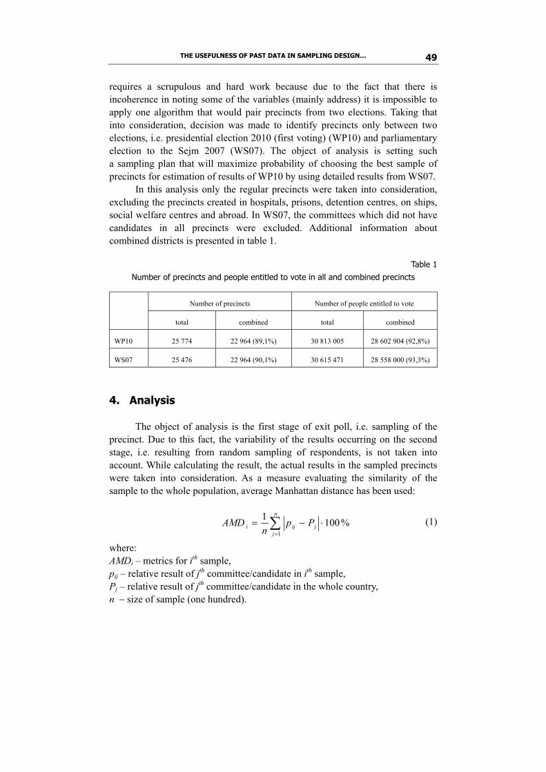
THE USEFULNESS OF PAST DATA IN SAMPLING DESIGN… 49
requires a scrupulous and hard work because due to the fact that there is incoherence in noting some of the variables (mainly address) it is impossible to apply one algorithm that would pair precincts from two elections. Taking that into consideration, decision was made to identify precincts only between two elections, i.e. presidential election 2010 (first voting) (WP10) and parliamentary election to the Sejm 2007 (WS07). The object of analysis is setting such a sampling plan that will maximize probability of choosing the best sample of precincts for estimation of results of WP10 by using detailed results from WS07.
In this analysis only the regular precincts were taken into consideration, excluding the precincts created in hospitals, prisons, detention centres, on ships, social welfare centres and abroad. In WS07, the committees which did not have candidates in all precincts were excluded. Additional information about combined districts is presented in table 1.
Table 1 Number of precincts and people entitled to vote in all and combined precincts
Number of precincts Number of people entitled to vote
total combined total combined
WP10 25 774 22 964 (89,1%) 30 813 005 28 602 904 (92,8%)
WS07 25 476 22 964 (90,1%) 30 615 471 28 558 000 (93,3%)
4. Analysis
The object of analysis is the first stage of exit poll, i.e. sampling of the precinct. Due to this fact, the variability of the results occurring on the second stage, i.e. resulting from random sampling of respondents, is not taken into account. While calculating the result, the actual results in the sampled precincts were taken into consideration. As a measure evaluating the similarity of the sample to the whole population, average Manhattan distance has been used:
%10011
⋅−= ∑=
n
jjiji Pp
nAMD (1)
where: AMDi – metrics for ith sample, pij – relative result of jth committee/candidate in ith sample, Pj – relative result of jth committee/candidate in the whole country, n – size of sample (one hundred).
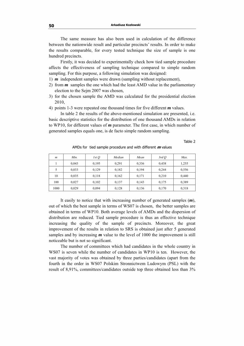
Arkadiusz Kozłowski 50
The same measure has also been used in calculation of the difference between the nationwide result and particular precincts’ results. In order to make the results comparable, for every tested technique the size of sample is one hundred precincts.
Firstly, it was decided to experimentally check how tied sample procedure affects the effectiveness of sampling technique compared to simple random sampling. For this purpose, a following simulation was designed: 1) m independent samples were drawn (sampling without replacement), 2) from m samples the one which had the least AMD value in the parliamentary
election to the Sejm 2007 was chosen, 3) for the chosen sample the AMD was calculated for the presidential election
2010, 4) points 1-3 were repeated one thousand times for five different m values.
In table 2 the results of the above-mentioned simulation are presented, i.e. basic descriptive statistics for the distribution of one thousand AMDs in relation to WP10, for different values of m parameter. The first case, in which number of generated samples equals one, is de facto simple random sampling.
Table 2
AMDs for tied sample procedure and with different m values
m Min. 1st Q Median Mean 3rd Q Max.
1 0,043 0,195 0,291 0,336 0,438 1,255
5 0,033 0,129 0,182 0,194 0,244 0,556
10 0,035 0,118 0,162 0,171 0,210 0,440
100 0,027 0,102 0,137 0,143 0,175 0,389
1000 0,029 0,094 0,128 0,136 0,170 0,318
It easily to notice that with increasing number of generated samples (m),
out of which the best sample in terms of WS07 is chosen, the better samples are obtained in terms of WP10. Both average levels of AMDs and the dispersion of distribution are reduced. Tied sample procedure is thus an effective technique increasing the quality of the sample of precincts. Moreover, the great improvement of the results in relation to SRS is obtained just after 5 generated samples and by increasing m value to the level of 1000 the improvement is still noticeable but is not so significant.
The number of committees which had candidates in the whole country in WS07 is seven while the number of candidates in WP10 is ten. However, the vast majority of votes was obtained by three parties/candidates (apart from the fourth in the order in WS07 Polskim Stronnictwem Ludowym (PSL) with the result of 8,91%, committees/candidates outside top three obtained less than 3%
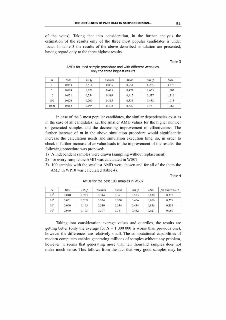
THE USEFULNESS OF PAST DATA IN SAMPLING DESIGN… 51
of the votes). Taking that into consideration, in the further analysis the estimation of the results only of the three most popular candidates is under focus. In table 3 the results of the above described simulation are presented, having regard only to the three highest results.
Table 3
AMDs for tied sample procedure and with different m values, only the three highest results
m Min. 1st Q Median Mean 3rd Q Max.
1 0,053 0,514 0,835 0,951 1,265 3,375
5 0,028 0,272 0,425 0,471 0,635 1,502
10 0,021 0,254 0,389 0,417 0,537 1,316
100 0,026 0,200 0,315 0,335 0,438 1,015
1000 0,012 0,195 0,302 0,329 0,431 1,067
In case of the 3 most popular candidates, the similar dependencies exist as
in the case of all candidates, i.e. the smaller AMD values for the higher number of generated samples and the decreasing improvement of effectiveness. The further increase of m in the above simulation procedure would significantly increase the calculation needs and simulation execution time, so, in order to check if further increase of m value leads to the improvement of the results, the following procedure was proposed: 1) N independent samples were drawn (sampling without replacement); 2) for every sample the AMD was calculated in WS07; 3) 100 samples with the smallest AMD were chosen and for all of the them the
AMD in WP10 was calculated (table 4). Table 4
AMDs for the best 100 samples in WS07
N Min. 1st Q Median Mean 3rd Q Max. for min(WS07)
103 0,040 0,223 0,344 0,371 0,523 0,830 0,375
104 0,061 0,209 0,324 0,350 0,466 0,806 0,278
105 0,060 0,195 0,310 0,334 0,434 0,846 0,434
106 0,060 0,193 0,307 0,341 0,432 0,927 0,060
Taking into consideration average values and quartiles, the results are
getting better (only the average for N = 1 000 000 is worse than previous one), however the differences are relatively small. The computational capabilities of modern computers enables generating millions of samples without any problem, however, it seems that generating more than ten thousand samples does not make much sense. This follows from the fact that very good samples may be

Arkadiusz Kozłowski 52
obtained already with a several thousand draws, however, these samples are not necessarily the most representative ones in the previous election.
In the last column of table 4 the AMDs for the best samples in WS07 are presented. In two cases out of four the values are higher than the average. Based on that, the conclusion may be drawn that the choice of the best sample out of N generated not always is the best solution. This situation is illustrated by graph 1 and 2.
0 1 2 3 4
0
1
2
3
4
WS07
WP
10
Graph 1. AMDs for N = 10 000 samples As it is clearly shown in graph 1, there is a dependence between AMD in
WS07 and AMD in WP10. However, the closer to the coordinate system’s origin, the weaker the dependence. Therefore, the samples which are the closest to X-axis (AMD in WS07) are not always the closest to Y-axis (AMD in WP10). The similar thing may be noticed in graph 2, where the best five hundred samples in WS07, sorted in the non-decreasing order, and their AMD in WP10 are presented. With the increase of the number of generated samples (N) the better samples in terms of the similarity to the general results in WP07 are obtained, however, the similarity of those samples to the general results in WP10 remains more or less the same and the values are pretty much dispersed.
Therefore, it seems justified to introduce modification to the tied sample procedure which would mean that not the best sample in terms of representativeness in the past election would be chosen to the survey but one out of one hundred to five hundred best samples would be selected. The more samples are generated (N) the more justified the modification seems to be. The issue that needs to be further analyzed is how this one sample should be chosen. Perhaps, there are attributes which will allow to separate samples which will remain representative in the subsequent elections from those which

THE USEFULNESS OF PAST DATA IN SAMPLING DESIGN… 53
representativeness will significantly deteriorate. The author compared turnout, the number of people entitled to vote and the variability of the results of particular committees in the best samples, however, no significant differences were identified.
..0 100 200 300 400 500
0.0
0.2
0.4
0.6
0.8
1.0
1.2
..0 100 200 300 400 500
0.0
0.2
0.4
0.6
0.8
1.0
1.2
..0 100 200 300 400 500
0.0
0.2
0.4
0.6
0.8
1.0
1.2
..0 100 200 300 400 500
0.0
0.2
0.4
0.6
0.8
1.0
1.2
Graph 2. AMDs for the best five hundred samples (sorted) out of N generated (□ - WP10, ● - WS07)
Another method to increase the representativeness of sample is applying stratified sampling. Based on the analysis of the differentiation of results in WS07, eight strata were identified using following features: territorial division of the country (two variants: north-western area including nine voivodeships and south-eastern area including seven voivodeships) and the type of subdivision (four variants: cities – municipalities with the number of people entitled to vote over eighty thousand, towns, other urban area, rural area). Allocation proportional to the average of relative share of two features: number of people entitled to vote and number of precincts in a stratum was applied (table 5).
N = 100 000 N = 1 000 000
N = 10 000 N = 1 000
AM
D
AM
D
AM
D
AM
D
sample sample
sample
samplesample

Arkadiusz Kozłowski 54
Table 5 Allocation of the sample
Cities Towns Other urban area Rural area
North-west 16 11 7 18
South-east 12 8 4 24
Subsequently, the stratified sampling was compared by simulation with
unrestricted sampling using also the relation to the past results. For this purpose ten thousand samples were drawn in accordance with every scheme and descriptive statistics with AMDs were calculated in the way it was done in the previous simulations (table 6). On average, thanks to stratified sampling more representative samples were obtained compared to unrestricted sampling. The same advantage of stratified sampling occurs when the elements of tied sample procedure are introduced, i.e. out of the previously generated ten thousand samples, the one hundred most representative in WS07 are chosen. The samples obtained by applying this method, with given N, turned out to be, on average, the most representative ones.
Table 6 Comparison of the results of simple random sampling simulation
and stratified sampling simulation for N=10 000 samples
Min. 1st Q Median Mean 3rd Q Max.
All samples
SRS 0,023 0,483 0,811 0,940 1,277 4,576
Stratified 0,036 0,471 0,783 0,859 1,180 3,108
The best 100 samples in terms of WS07
SRS 0,061 0,209 0,324 0,350 0,466 0,806
Stratified 0,073 0,207 0,292 0,320 0,401 0,860
The last aspect of exit poll is an intentional omission of the smallest
precincts in sampling procedure. Such behaviour from the research institution’s point of view is acceptable due to financial benefits because while surveying the smaller number of large precincts, the same sample of respondents may be obtained with lower costs. Obviously, intentional exclusion of some of the units out of the sampling population affects the estimates. This fault, however, can be eliminated if tied sample procedure is applied, because the sample is chosen in such way that it reflects the total result, which also includes the precincts omitted in sampling. In table 7 the characteristics of the best one hundred (in terms of accuracy in WS07) out of ten thousand generated samples are presented, the number of sampling population was reduced in the subsequent rows by the precincts with the number of people entitled to vote smaller than k.

THE USEFULNESS OF PAST DATA IN SAMPLING DESIGN… 55
Table 7 AMDs for the best 100 samples out of 10 000, with the omission
of precincts smaller than k
k Min. 1st Q Median Mean 3rd Q Max.
500 0,048 0,216 0,342 0,348 0,465 0,872
600 0,024 0,213 0,319 0,338 0,434 0,821
700 0,025 0,197 0,277 0,316 0,409 0,802
800 0,061 0,229 0,321 0,345 0,437 0,932
900 0,028 0,228 0,345 0,366 0,491 0,822
1000 0,029 0,186 0,307 0,322 0,405 0,871
1100 0,059 0,217 0,349 0,368 0,465 0,862
1200 0,068 0,217 0,344 0,365 0,477 1,039
1300 0,073 0,231 0,401 0,423 0,560 1,162
1400 0,098 0,319 0,454 0,473 0,584 1,094
1500 0,109 0,336 0,474 0,534 0,696 1,222
2000 0,070 1,090 1,286 1,269 1,487 1,834
The above results show that in case of WP10 the omission of precincts
smaller than six hundred to eight hundred people entitled to vote would not reduce the representativeness of sample but, in fact, it would increase it. Even limiting the sampling population only to precincts larger than one thousand people entitled to vote would not involve the loss of quality of the sample if the tied sample procedure is applied. 5. Conclusions
The detailed data about the past elections results is a valuable source of additional information enabling the improvement of sampling in exit poll. Based on the full results of the presidential election 2010 and the parliamentary election to the Sejm 2007 it was proven by means of simulation experiments that applying tied sample procedure significantly improves the representativeness of the sample. This benefit increases along with the growth of the number of generated samples. However, the more samples are generated the more advisable it is to modify the procedure in a way that instead of choosing the best sample from the past election, the choice is made from the first several hundred samples. The method of this choice requires further analysis. The improvement was obtained by applying stratified sampling in which the population was divided to eight strata based on two variables: geographic division and the type of territorial unit. It was also proven that by applying tied sample procedure the smallest precincts may be omitted in the survey, which is beneficial from financial and organizational point of view and does not further affect the results.

Arkadiusz Kozłowski 56
Acknowledgements
The author would like to thank Prof. Mirosław Szreder for the inspiration to conducting the research and valuable comments when writing the article and Mirosław Bogdanowicz from Krajowe Biuro Wyborcze for sharing the data in the useful format.
References Andreenkova, A., Moreno, A. (2008) Using exit polls to do more than project
outcomes: the role and functions of exit polls in advanced and new democracies. 3MC Conference Proceedings, Berlin.
Barreto, M.A., et al. (2006) Controversies in exit poll. “Political Science and Politics” Vol. 39, No. 3, 477-483.
Bishop, G.F., Fisher, B.S. (1995) “Secret ballots” and self-reports in an exit-poll experiment. “Public Opinion Quarterly” Vol. 59, No. 4, 568-588.
Busch, R.J., Lieske, J.A. (1985) Does time of voting affect exit poll results? “Public Opinion Quarterly” Vol. 49, No. 1, 94-104.
Curtice, J., Firth, D. (2008) Exit Polling in a Cold Climate: The BBC-ITV Experience in Britain in 2005 [with Discussion]. “Journal of the Royal Statistical Society. Series A (Statistics in Society)” Vol. 171, No. 3, 509- -539.
Frankovic, K.A. (1992) Technology and the Changing Landscape of Media Polls, in: T.E. Mann, G.R. Orren (eds) “Media Polls in American Politics”. Brookings Institution, Washington, DC.
Hilmer, R. (2008) Exit polls – a lot more than just a tool for election forecasts, in: M. Carballo, U. Hjelmar (eds.) “Public opinion polling in a globalized World”. Springer, Berlin.
Hofrichter, J. (1999) Exit polls and elections campaigns, in: B.I. Newman, (ed.) “Handbook of political marketing”. Thousand Oaks, Sage Publications.
Klorman, R. (1976) What Time Do People Vote? “The Public Opinion Quarterly” Vol. 40, No. 2, 182-193.
Lenski, J. (2008) New methodological Issues in conducting exit polls. 3MC Conference Proceedings, Berlin.
Levy, M.R. (1983) The methodology and performance of election day polls. “Public Opinion Quarterly” Vol. 47, No. 1, 54-67.

THE USEFULNESS OF PAST DATA IN SAMPLING DESIGN… 57
Moore, D.W. (2003) New Exit Poll Consortium Vindication for Exit Poll Inventor Inside the polls, Gallup, http://www.gallup.com/poll/9472/new-exit-poll-consortium-vindication-exit-poll-inventor.aspx (30.09.11).
Seymour, S. (1986) Do exit polls influence voting behavior. “Public Opinion Quarterly” Vol. 50, No. 3, 331-339.
Szreder, M. (2007) O roli informacji spoza próby w badaniach sondażowych. “Przegląd Socjologiczny” LVI/1, 97-107.
Ustawa z dnia 16 lipca 1998 r., Ordynacja wyborcza do rad gmin, rad powiatów i sejmików województw. Dz. U. 1998, nr 95, poz. 602, art. 30.
UŻYTECZNOŚĆ DANYCH Z PRZESZŁOŚCI DLA PLANU LOSOWANIA W BADANIACH
TYPU EXIT POLL
Streszczenie
Głównym zadaniem exit poll jest predykcja wyniku wyborczego tuż po zamknięciu lokali wyborczych. Nie mniej ważnym celem badania jest oszacowanie rozkładów głosów w różnych przekrojach społeczno-demogra-ficznych. Kluczową kwestią dla jakości tych oszacowań jest wybór odpo-wiedniej próby obwodów głosowania. W artykule poddane zostały analizie alternatywne do losowania prostego metody doboru próby obwodów. Główny nacisk położono na wykorzystanie powszechnie dostępnych baz danych ze szczegółowymi wynikami przeszłych wyborów. Za pomocą eksperymentów symulacyjnych oceniono efektywność techniki powiązania wyboru nowej próby z przeszłymi wynikami (tied sample procedure) oraz wskazano optymalne dla niej parametry, a także zaproponowano pewną modyfikację procedury. Najlepsze wyniki uzyskano dla losowania warstwowego z zastosowaniem elementów procedury tied sample. Wskazano również możliwość redukcji kosztów badania bez straty na efektywności poprzez odpowiedni dobór wy-łącznie dużych obwodów.

Jan Kubacki Alina Jędrzejczak
THE COMPARISON OF GENERALIZED VARIANCE FUNCTION WITH OTHER METHODS
OF PRECISION ESTIMATION FOR POLISH HOUSEHOLD BUDGET SURVEY
1. Introduction In the recent years, the demand for reliable small area estimates has
significantly increased all over the world. It is mainly due to its growing use in formulating policies, the allocation of government funds and in the regional planning. Creating reliable estimates for small areas, where sample size is substantially lower than for the whole country (for example for counties – in Poland NUTS4) is a great challenge for statisticians. The problems can arise not only with the reliable direct estimates for small areas but with the assessment of their precision as well. Even when administrative data are available that can be used as auxiliary information to increase the precision of direct estimates, there might not be the sample sizes large enough for particular units to enable the reliable estimation of standard errors. In such a case, an approximate technique for variance estimation called Generalized Variance Function (GVF) can be a good choice.
In the Polish literature there are relatively few publications that discuss GVF approach in the context of small area estimation. However, during the last two decades, some publications concerning estimation for counties were presented. Here we can mention the papers by Bracha, Lednicki and Wieczorkowski (2003, 2004), Gołata (2004), Kordos (2004) and Kubacki (1999, 2006) that summarize the results of estimation for counties obtained on the basis of Polish Labor Force Survey. Another important work in this field was the report entitled “Social Exclusion and Integration in Poland: An Indicators-based Approach” prepared for UNDP (2006), where data from Polish Household Budget Survey (also for counties) were used. The concept and the results presented in the report can be considered pioneer in Polish literature and may be useful in practice whenever the estimates for counties are needed.

THE COMPARISON OF GENERALIZED VARIANCE FUNCTION… 59
Generalized Variance Function approach is widely known in the subject literature. Here we can mention the papers of Cho et al. (2002) and of Johnson and King (1987), U.S. Department of Education, Office of Educational Research and Improvement (1995), and the textbooks by Lohr (1999) and Wolter (1985).
The main advantage of the method is its simplicity and the reduction of publication costs (also in the small area case, when the amount of estimates may be large). The approximations of sampling errors are simplified for a variety of estimates that are typically generated from a survey with a large number of variables. Another advantage of GVF approach is its stability that can reduce the unreliable values for some cases (the method can produce more stable sampling error estimates by averaging over time and generalizing in some way).
In the paper we present in detail the results of the application of Generalized Variance Function to the small area estimation in Poland, comparing with other direct variance estimation methods.
2. Outline of direct variance estimation methods applied
in the paper The basic concept of the replication approach applied to the variance
estimation is repeatable selection of subsamples from the whole sample. The variance of a statistic based on the whole sample can be obtained using the variability of the estimates that arise from the subsamples. Replication techniques are often used in applications concerning complex survey designs, complicated estimators and when complex weight structure is used. An important advantage of replication methods is their simplicity. It is connected with the simplicity of procedures which can be applied to the estimation of means, proportions, totals, correlations and so on. Another advantage is the possibility of modification of design weights caused by non-response or post-stratification. This modification can be easily applied comparing with some analytical formulas.
Some disadvantage of replication techniques is their computational complexity, however in the case of modern computer systems this impediment can be easily overcome, especially for data files of medium size, as in most sample survey cases. There is also a disadvantage related to inadequate selection of subsamples for complex sampling designs. In such a case, when subsamples do not reflects the sample design, the results obtained in this way may be seriously biased.
Replication techniques can be implemented using the following schema. – At the first step, subsamples selection that corresponds to the sample
allocation among strata should be carried out. Often, as in the BRR and Fay method, there should be two subsamples in each stratum. This requirement is

Jan Kubacki, Alina Jędrzejczak 60
not always met for small areas (in particular for counties), what makes the variance estimation more difficult. In such a case, other estimation techniques should be used.
– At the second step, the replication weights are computed, using the methods similar to the ones used for the whole sample.
– At the third step, the estimation for the subsamples is conducted using the same method as for the whole sample.
– At the final step, the variance for the whole sample is computed, using the whole sample and subsamples results.
The variance of θ is computed using the following formula:
∑=
⎟⎠⎞⎜
⎝⎛=
A
1
2ˆ-ˆc)ˆV(
αα θθθ (1)
where: θ – Is the parameter of interest,
θ – is the parameter estimate θ for the whole sample,
aθ – is the parameter estimate θ for the replicate a, A – is the number of replicates, c I –s constant that depends on the replication method.
Values of the parameter c for different variants of replication methods are
summarized in the table 1.
Table 1 Replication methods and the value of parameter “c”
Method Abbreviation Value of parameter c
Balanced Repeated Replication BRR 1/A
Fay’s method FAY 1/(A(1-k)2)
Jackknife 2 JK2 1
Bootstrap - 1/(A-1)
Balanced Repeated Replication
Balanced Repeated Replication is the method most often used for multi-stage and multi-strata sampling designs. In the simplest version the whole population is divided into L strata, and for each stratum two subsamples are chosen. Each replicate half-sample estimate is formed by selecting one of the two subsamples from each stratum based on a Hadamard matrix and then using only the selected subsample to estimate the parameter of interest. In the case of
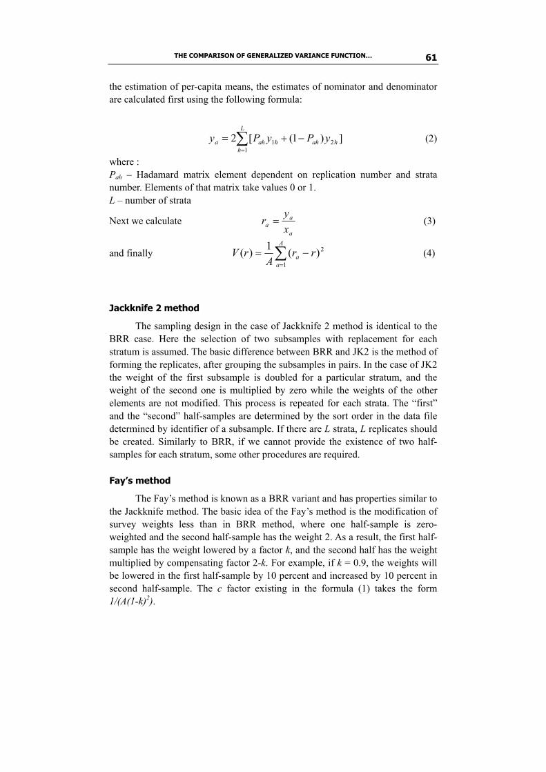
THE COMPARISON OF GENERALIZED VARIANCE FUNCTION… 61
the estimation of per-capita means, the estimates of nominator and denominator are calculated first using the following formula:
∑=
−+=L
hhahhaha yPyPy
121 ])1([2 (2)
where : Pah – Hadamard matrix element dependent on replication number and strata number. Elements of that matrix take values 0 or 1. L – number of strata
Next we calculate a
aa x
yr = (3)
and finally ∑=
−=A
aa rr
ArV
1
2)(1)( (4)
Jackknife 2 method
The sampling design in the case of Jackknife 2 method is identical to the BRR case. Here the selection of two subsamples with replacement for each stratum is assumed. The basic difference between BRR and JK2 is the method of forming the replicates, after grouping the subsamples in pairs. In the case of JK2 the weight of the first subsample is doubled for a particular stratum, and the weight of the second one is multiplied by zero while the weights of the other elements are not modified. This process is repeated for each strata. The “first” and the “second” half-samples are determined by the sort order in the data file determined by identifier of a subsample. If there are L strata, L replicates should be created. Similarly to BRR, if we cannot provide the existence of two half-samples for each stratum, some other procedures are required. Fay’s method
The Fay’s method is known as a BRR variant and has properties similar to the Jackknife method. The basic idea of the Fay’s method is the modification of survey weights less than in BRR method, where one half-sample is zero-weighted and the second half-sample has the weight 2. As a result, the first half-sample has the weight lowered by a factor k, and the second half has the weight multiplied by compensating factor 2-k. For example, if k = 0.9, the weights will be lowered in the first half-sample by 10 percent and increased by 10 percent in second half-sample. The c factor existing in the formula (1) takes the form 1/(A(1-k)2).

Jan Kubacki, Alina Jędrzejczak 62
Overview of bootstrap method
As the jackknife, the bootstrap method is connected with a broader range of issues than survey sampling. It is also applied in hypothesis testing, and the construction of classification and regression models. This method may be preliminarily described assuming that a sample was drawn by means of a simple random sampling with replacement. In such a case an original sample is treated as a population and the samples (called bootstrap samples) are selected from it. By creating subsamples from the original sample using the same sampling design we can expect them to imitate the properties of the whole population. Such an approach was first devised by Efron (1979), but the detailed description of the method can be found in Efron and Tibshirani (1993). The bootstrap method was applied in the paper because for some sampling units only one stratum was chosen and the sampling design was similar to the simple random sampling. For larger units, the BRR method was used, that naturally mimics the original sampling design. This is valid in particular for larger cities.
In the simplest case determining the sampling variance by means of the bootstrap method can be described as follows: – Draw independently A = 500 simple random samples (with replacement) from
the whole sample of size n. – Using the selected “bootstrap” samples, calculate the values of the parameter
a*θ using the same formula as for the whole sample. – Determine the estimate of the estimator variance using the following formula
∑=
−−
=A
a
a
AV
1
2* )ˆˆ(1
1)ˆ(ˆ θθθ (5)
Generalized Variance Function approach
The method assumes that a simple model is constructed that allows us to determine the precision estimate on the basis of the parameter estimate itself. The procedure can be described as follows.
Using replication or another variance estimation method, the variances of k parameters, described as should be obtained. Assuming vi be the variance of the estimator of the form:
(6)
one can propose a model, that links the values of vi and. In most cases the model is as follows:
(7)
kttt ˆ,...,ˆ,ˆ21
22 )ˆ(ˆ/)ˆ( iiii tCVttVv ==
it
itvi
βα +=

THE COMPARISON OF GENERALIZED VARIANCE FUNCTION… 63
Using well known regression techniques, the regression coefficients α and β can be estimated. The last step is to determine the standard estimation error on the basis of regression equation. 3. Results of Comparison of Generalized Variance Function with other Variance Estimation Methods
As it has been seen in the table 2, the models obtained for different
income variables have relatively good statistical properties, however some of them fits the data slightly less. This is particularly due to outlier existence (as in the available income case – see table 3) and due to the nature of variables that describe rare attributes (as for other income). Table 3 includes GVF estimates for a model without constant. Such a model was chosen because of some difficulties with fitting the values using the model with constant. In such a case GFV values for higher direct estimate values are overestimated, and sometimes the dependence has reversed character (for lower estimate values, lower GVF values are obtained), what is undesirable.
Table 2 Summary of GVF models for different income variables
on the basis of county estimates from Polish Household Budget Survey
Variable R-square F-statistic
Available income 0,277 133,34
Income from hired work 0,554 432,13
Income from self-employment 0,343 174,10
Income from social security benefits 0,437 269,76
Retirement pays 0,653 656,07
Pensions resulting from inability to work 0,617 560,41
Family pensions 0,574 434,50
Income from other assistance benefits 0,513 367,31
Unemployment benefits 0,558 373,08
Other income 0,247 114,17
Other income of which gifts 0,259 121,63
The variance estimates obtained by means of GVF are usually greater than
the corresponding replicate estimates and also in most cases greater than the bootstrap estimates. However, looking at the example presented in the table 3 one can easily notice that there are some direct values that are greater than the corresponding GVF estimates. This confirms the stability of GVF estimates which may be particularly useful when variance estimates for small area models are needed. Please note, that for some counties, there are no values of variance

Jan Kubacki, Alina Jędrzejczak 64
estimates obtained using various replication techniques. It comes by the fact, that in some strata there is only one PSU. Analyzing in detail the results presented in the table 3, one can also observe significantly lower CV values for replication and bootstrap methods that were obtained for Warsaw (grey highlighted). This observation suggests applying General Variance Function for large cities separately from the remaining part of the sample.
Table 3 Estimated values of CV for available income by counties in mazowieckie region using
Balanced Repeated Replication (BRR), Jackknife (JK2), Fay, Bootstrap and GVF
Coefficient of variation
County
Direct available income estimate
BRR Jack nife
(JK2) Fay Boot-
strap
Boot-strap with deff
GVF
Białobrzeski 389,34 - - - 23,20 36,34 14,98 Ciechanowski 619,20 25,34 10,37 15,68 6,64 10,39 11,88 Garwoliński 494,72 5,71 5,71 5,65 5,84 9,15 13,29 Gostyniński 504,84 - - - 11,83 18,53 13,16 Grodziski 785,14 12,65 11,94 12,59 11,76 18,42 10,55 Grójecki 769,03 - 35,67 17,07 10,27 16,09 10,66 Legionowski 1163,9 - - - 13,71 21,47 8,67 Lipski 506,09 - - - 20,99 32,88 13,14 Łosicki 516,52 - - - 19,37 30,33 13,01 Makowski 490,83 11,43 6,92 8,82 9,38 14,69 13,34 Miński 636,72 - 28,00 16,43 7,62 11,93 11,71 Mławski 516,28 5,86 6,84 5,56 8,12 12,72 13,01 Nowodworski 635,86 17,45 13,08 12,21 5,29 8,29 11,72 Ostrowski 552,91 - - - 12,25 19,19 12,57 Otwocki 690,89 7,47 4,83 5,94 4,04 6,32 11,25 Piaseczyński 835,07 0,87 1,34 1,23 8,10 12,68 10,23 Płocki 543,07 17,42 24,03 8,89 7,78 12,19 12,68 Płoński 513,08 8,99 8,89 8,99 9,49 14,86 13,05 Pruszkowski 875,50 7,49 5,92 6,54 5,51 8,62 9,99 Przysuski 499,16 - - - 14,50 22,71 13,23 Pułtuski 529,85 - - - 13,85 21,70 12,84 Radomski 492,58 5,17 5,47 3,57 4,15 6,49 13,32 Siedlecki 536,47 - - - 8,11 12,71 12,76 Sierpecki 528,71 - - - 11,51 18,03 12,86 Sochaczewski 756,45 14,37 15,18 12,43 11,51 18,02 10,75 Sokołowski 452,88 - - - 14,72 23,06 13,89 Szydłowiecki 550,45 4,30 4,60 6,25 5,57 8,72 12,60 Warszawski 1311,6 2,94 3,02 2,99 1,82 2,84 8,16 Warszawski zachodni 1356,0 - - - 20,24 31,70 8,02 Węgrowski 616,87 3,04 3,01 3,04 12,78 20,01 11,90 Wołomiński 694,99 17,78 16,72 15,98 7,10 11,13 11,21 wyszkowski 555,52 - - - 10,28 16,11 12,54 Zwoleński 722,25 - - - 16,04 25,11 11,00 Żuromiński 480,75 - - - 14,18 22,20 13,48 Żyrardowski 733,43 2,02 2,14 1,53 4,58 7,18 10,92 m. Ostrołęka 742,94 - - - 7,93 12,42 10,85 m. Płock 772,05 - - - 6,92 10,83 10,64 m. Radom 628,53 2,61 1,75 2,28 3,79 5,94 11,79 m. Siedlce 771,01 13,80 18,79 8,29 5,90 9,23 10,65
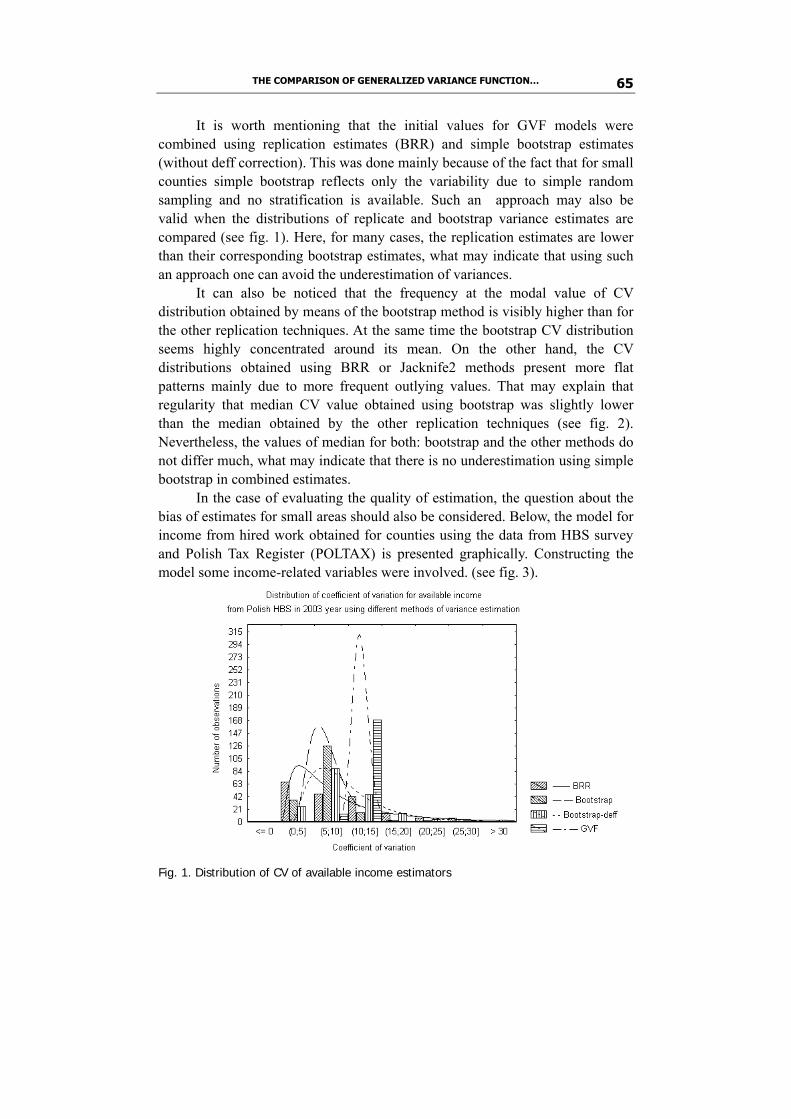
THE COMPARISON OF GENERALIZED VARIANCE FUNCTION… 65
It is worth mentioning that the initial values for GVF models were combined using replication estimates (BRR) and simple bootstrap estimates (without deff correction). This was done mainly because of the fact that for small counties simple bootstrap reflects only the variability due to simple random sampling and no stratification is available. Such an approach may also be valid when the distributions of replicate and bootstrap variance estimates are compared (see fig. 1). Here, for many cases, the replication estimates are lower than their corresponding bootstrap estimates, what may indicate that using such an approach one can avoid the underestimation of variances.
It can also be noticed that the frequency at the modal value of CV distribution obtained by means of the bootstrap method is visibly higher than for the other replication techniques. At the same time the bootstrap CV distribution seems highly concentrated around its mean. On the other hand, the CV distributions obtained using BRR or Jacknife2 methods present more flat patterns mainly due to more frequent outlying values. That may explain that regularity that median CV value obtained using bootstrap was slightly lower than the median obtained by the other replication techniques (see fig. 2). Nevertheless, the values of median for both: bootstrap and the other methods do not differ much, what may indicate that there is no underestimation using simple bootstrap in combined estimates.
In the case of evaluating the quality of estimation, the question about the bias of estimates for small areas should also be considered. Below, the model for income from hired work obtained for counties using the data from HBS survey and Polish Tax Register (POLTAX) is presented graphically. Constructing the model some income-related variables were involved. (see fig. 3).
Fig. 1. Distribution of CV of available income estimators
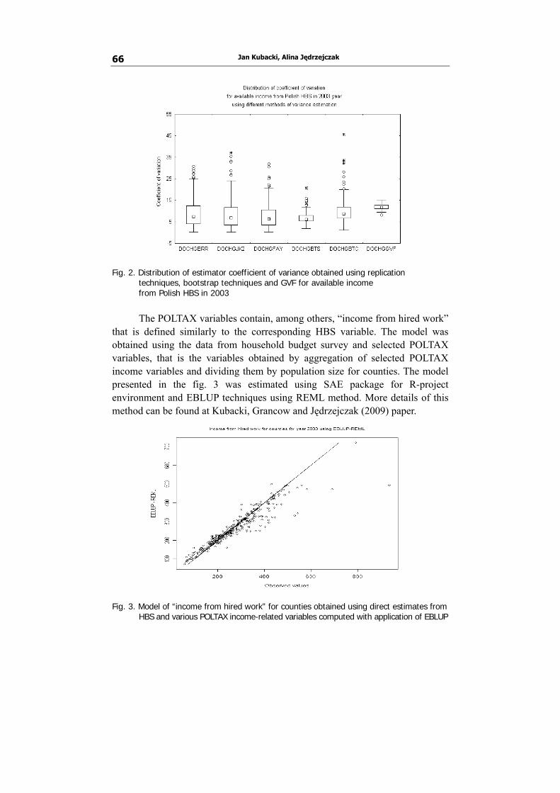
Jan Kubacki, Alina Jędrzejczak 66
Fig. 2. Distribution of estimator coefficient of variance obtained using replication
techniques, bootstrap techniques and GVF for available income from Polish HBS in 2003
The POLTAX variables contain, among others, “income from hired work”
that is defined similarly to the corresponding HBS variable. The model was obtained using the data from household budget survey and selected POLTAX variables, that is the variables obtained by aggregation of selected POLTAX income variables and dividing them by population size for counties. The model presented in the fig. 3 was estimated using SAE package for R-project environment and EBLUP techniques using REML method. More details of this method can be found at Kubacki, Grancow and Jędrzejczak (2009) paper.
Fig. 3. Model of “income from hired work” for counties obtained using direct estimates from
HBS and various POLTAX income-related variables computed with application of EBLUP
THE COMPARISON OF GENERALIZED VARIANCE FUNCTION… 67
Graphical examination of the results reveals that the estimates obtained by means of the methods presented above present relatively good consistency with the population data and are not seriously biased. This may indicate that the method may also be used in the future. 4. Conclusions
The results presented in the paper confirm that it is possible to obtain
reliable income-related estimates for counties, using the data from Household Budget Survey. The Generalized Variance Function approach allows us not only to obtain relatively stable estimates of estimation errors but also makes it possible to provide the estimation for counties that are not present in HBS sample and can only be treated using small area models. However, a special care should be taken, when the analysis is performed for more detailed variables. It would therefore be advisable to use a combined method of variance estimation in that case. Further examination of other direct methods of precision estimation, as Jackknife Repeated Replication or Sampling with over-replacement, using as an input the variances that arise from GVF models, may be considered in the future studies. Also a more detailed discussion of small area models using precision values obtained by means of GVF technique should be conducted in the future. References Bracha C., Lednicki B., Wieczorkowski R. (2003) Estimation of Data from the
Polish Labour Force Surveys by poviats (counties) in 1995-2002 (in Polish). GUS, Warszawa.
Bracha C., Lednicki B., Wieczorkowski R. (2004) Application of complex estimation methods to the disaggregation of data from Polish Labour Force Survey in 2003 (in Polish). GUS, Warszawa.
Cho, M.J., Eltinge, J.L., Gershunskaya, J., Huff, L. (2002) Evaluation of Generalized Variance Function Estimators for the U.S. Current Employment Survey. Proceedings of the American Statistical Association, Survey Research Methods Section, 534-539.
Efron, B., (1979) Bootstrap methods: another look at the jackknife. Annals of Statistics 7, 1-26.
Efron, B. and Tibshirani, R.J. (1993) An Introduction to the Bootstrap. Chapman & Hall, New York.

Jan Kubacki, Alina Jędrzejczak 68
Gołata, E. (2004a) Problem of Estimating Unemployment for Small Domains in Poland. “Statistics in Transition” 6, 755-776.
Johnson, E.G., and King, B.F. (1987) Generalized variance functions for a complex sample survey. “Journal of Official Statistics” 3, 235-250.
Kordos, J. (2005) Some Aspects of Small Area Statistics and Data Quality. “Statistics in Transition” Vol. 7, No. 1, 63-83
Kubacki, J. (1999) Evaluation of Some Small Area Methods for Polish Labour Force Survey in one Region of Poland. Proceedings of the IASS Satellite Conference on Small Area Estimation, Riga, Latvia, 245-249.
Kubacki, J. (2006) Remarks on the Polish LFS and Population Census Data for Unemployment Estimation by County. “Statistics in Transition” Vol. 7, No. 4, 901-916.
Kubacki J., Grancow B., Jędrzejczak A. (2009) An example of empirical best linear unbiased predictor (EBLUP) application for small area estimation in Polish Household Budget Survey, 9-20, Proceedings from conference “Survey Sampling in Economic and Social Research” organized by University of Economics in Katowice in 2008.
Lohr, S. (1999) Sampling: Design and Analysis. Duxbury Press.
Rao, P.S.R.S. (2001) Sampling Methodologies with Applications. Chapman and Hall/CRC.
UNDP Poland (2006) Social Exclusion and Integration in Poland: An Indicators-based Approach. Warsaw.
U.S. Department of Education, Office of Educational Research and Improvement (1995) Design Effects and Generalized Variance Functions for the 1990-1991 Schools and Staffing Survey (SASS), February 1995.
Wolter, K.M. (1985) Introduction to Variance Estimation. Springer-Verlag, New York.
PORÓWNANIE METODY UOGÓLNIONEJ
FUNKCJI WARIANCYJNEJ Z INNYMI METODAMI SZACOWANIA PRECYZJI DLA BADANIA
BUDŻETÓW GOSPODARSTW DOMOWYCH
Streszczenie
Wariancja lub współczynnik zmienności estymatora mogą być przed-stawione jako funkcje jego wartości oczekiwanej z użyciem zależności znanej

THE COMPARISON OF GENERALIZED VARIANCE FUNCTION… 69
jako uogólniona funkcja wariancyjna. W artykule przedstawiono rezultaty obli-czeń dla szacunków precyzji obejmujących różne kategorie dochodu wyznaczone dla powiatów. Podstawą obliczeń były dane pochodzące z Badania Budżetów Gospodarstw Domowych. Rezultaty otrzymane metodą uogólnionej funkcji wariancyjnej zostały porównane z innymi uproszczonymi metodami szacowania wariancji.
Jako punkt wyjścia przyjęto metodę szacowania wariancji z użyciem zrównoważonych półprób replikacyjnych (tzw. BRR) oraz metodę bootstrapową, gdy zastosowanie metody BRR było niemożliwe. W celu określenia modelu dla uogólnionej funkcji wariancyjnej użyto funkcji hiperbolicznej. Obliczenia prze-prowadzono, stosując program WesVAR oraz SPSS, jak również własne pro-cedury obliczeniowe przygotowane dla pakietu R-project. Oszacowano również zgodność szacunków dla powiatów z użyciem modeli dla małych obszarów oraz danych administracyjnych.

Dorota Raczkiewicz SOME ASPECTS OF POST ENUMERATION SURVEYS
IN POPULATION CENSUSES IN POLAND
AND GERMANY
1. Introduction
Population census is valuable data source of population and its structure. Although as every statistical survey, a census is not perfect quality and is biased of errors. Errors in the census results are classified into two general categories: coverage errors and content errors. Coverage errors are the errors that arise due to omissions or duplications of persons or housing units in the census enumeration. Content errors are errors that arise in the incorrect reporting or recording of the characteristics of persons, households and housing units enumerated in the census. Both kinds of errors can be assess by post enumeration survey. Population censuses in Poland and Germany conducted in this year have the similar methodology, both censuses are register based and random sample surveyed. Also both countries conducted post enumeration surveys several weeks after the main census. There are very detailed recommendation how to carry out the population census and the post enumeration surveys, proposed by EUROSTAT and UN. Poland and Germany comply with these recommendation in different degree.
The aim of this paper is to compare post enumeration surveys and population censuses in Poland and Germany, to present problem with data quality and potential errors of censuses and to point at international recommendation on quality assessment of population censuses according to the UN and EUROSTAT. 2. Comparison of population censuses in Poland and Germany
The population census provides the most detailed information about population and its territorial distribution, demographic structure, social and professional, as well as socio-economic characteristics of households and families,

SOME ASPECTS OF POST ENUMERATION SURVEYS IN POPULATION CENSUSES… 71
and their resources, and housing conditions at all levels of territorial division of the country: national, regional and local level.
Population censuses are conducted in Poland and in the world about every ten years. Population censuses are the largest statistical projects in all countries. In this year population censuses were conducted both in Poland and in Germany. In both countries these censuses has the special capacity. In Poland because it is the first census since Poland became an EU member state. This implies a series of commitments, including need to provide information in the social-demographic and socio-economic, to the extent and time limits set by the European Commission. In Germany because this is the first population census after the Berlin Wall fell and unification of two parts of Germany, many people moved from east to west and European integration has progressed rapidly. In the former territory of the Federal Republic of Germany, the last complete enumeration was held in 1987, in the GDR a population census was taken in 1981. Ever since, the official number of population has been determined using a statistical method called intercensal population updates.
In both countries population censuses were performed a register-based censuses. Nowadays because of high technological progress a lot of data are stored in many administrative registers, data bases and state reports of some institution. These sources of data contain comparable information.
In both censuses there are collected information on buildings and housing, on households and on people. In Germany there are two surveys: the Census of Buildings and Housing and the Household Surveys. In the Census of Buildings and Housing, all 17.5 million owners of residential property receive a questionnaire by post by the reference date. The questionnaire will request information on residential buildings and dwellings, such as the year of construction, type of building, equipment, floor space and number of rooms. In the Household Surveys in Germany, 10 percent of the population were interviewed by interviewers on or after 9 May 2011. The respondents in Germany were selected randomly. In Poland 20 percent were also selected randomly, using stratified sampling, strata were created on the basis of information from administrative registers and state territorial register (TERYT). In both censuses people were requested to provide information also on their education and training, employment and migration.
Both countries used a mixed-mode method for data collection from multiple sources and combines a complete enumeration with sample surveys. Interview by: – CAPI – Computer Assisted Personal Interview; – Self registration by Internet: CAII – Computer Assisted Internet Interview; – CATI – Computer Assisted Telephone Interview.
Both the Central Statistical Office in Poland and the Federal Statistical Office in Germany provide individual data protection.

Dorota Raczkiewicz 72
3. Data quality and potential errors in population censuses
Population census such as other statistical survey is not perfect quality and
errors can and do occur at all stages of the census operation. Statistical data are high quality if they are accessible and clarified, relevant, on time and punctual, comparable, coherent and accurate.
Accessibility and clarity means that data are easily accessible and available in forms suitable to the users, users know how to get the data, and the data provider help users in interpreting the results and gives data in proper formats etc. Relevance is the degree to which statistics meet current and potential users’ needs. Timeliness and punctuality means that data are available in short time. Comparability is then it is possibly to compare data between countries and different time of periods. To ensure comparability of the results at European level, all member states have to provide information on a specified range of variables with unified definitions and classifications. Coherence is when data are adequate to be reliably combined in different ways and for various uses. Accuracy is the most important feature of statistical data and expresses the closeness of the true value. True value, which in practice is not known, is a value that is obtained that, if the data were collected and analysed without any errors for all units of the target population.
The data would be accurate if a full-scale survey were perfectly conducted and all relevant conditions of the survey were perfect. The perfect conditions depend on specification of the study object, socio-political situation of the country, methods of data collection, used statistical procedures, including methods of estimation, qualifications of personnel involved in the study (interviewers, controllers, people that coding and inputting data, research period, treatment of the questions and explanations, used definitions etc.).
The data accuracy depends on sampling and non-sampling errors. Previous censuses were full scale surveys with no probability mechanism, full population was interviewed, no sample was selected, so no sampling errors arose. The situation is different in this year censuses in Poland and Germany, where respectively 20 and 10 percent samples were drawn from population. And sampling errors must be taken into consideration. In additional, it appear the problem with combining data from two sources: survey data and register data. Registers can be also inaccurate and they are a source of some kind of errors.
Non-sampling errors occur in every survey, both census and sample survey and they can arise in particular stages of the survey and census, beginning from planning the survey and ending on making the survey results available to users. There are two kinds of non-sampling errors: completeness errors and content errors. The completeness errors are coverage errors (omission,

SOME ASPECTS OF POST ENUMERATION SURVEYS IN POPULATION CENSUSES… 73
duplication and erroneous inclusion of unit) and non response (not location, absence at home, no contact, refusals, lost questionnaires, questionnaires discarded during the inspection). Errors of contents are response errors (caused by respondent, interviewer, during recording and copying data), data processing errors (during coding, input and editing, table creation and calculations), errors of analysis and presentation of results (incorrect methods of analysis, misinterpretation, erroneous statistical inference, incorrect presentation of the results), (Kordos, 1988).
4. Post enumeration surveys in population censuses
in Poland and Germany There are a lot of methods to assess the quality of population census:
– Quality control techniques such as internal consistency checks; – Comparisons of results with other data sources including previous censuses,
current household surveys, and/or administrative records; – Record-checking, in which individual census records are matched against
alternative sources and specific data items are checked for accuracy; – Some evaluations analyze, interpret, and synthesize the effectiveness of
census components and their impact on data quality or census coverage; – Post-enumeration surveys are used to estimate census coverage error; – Post-census surveys designed to measure content error are usually known as
re-interview surveys; – Ethnographic and social network methods provide a way to study the effects
of mobility on census coverage or to measure census coverage of specific subpopulations.
In this paper special attention is paid to post-enumeration survey, conducted after 2011 population census both in Poland and Germany. In the post-enumeration survey in 2011 population census in Germany, 5% of all participants of the survey households are asked a few weeks after the first interview a second time by other interviewers then in the household survey. Such checks on survey results are internationally accepted and allow an assessment of the quality of the results from the survey households. In principle, again the same issues as the survey households are made, but there are less questions. The survey follows the same procedure as the households survey, only with different interviewers. It is also responsible for this survey in some provinces opposed to collection agency, but the State Statistical Office. Even with follow-up survey, we naturally offer the opportunity to complete either the questionnaire alone and returned to the State Statistical Office or the Designated collection agency or to report the information online. For reasons of data protection, a transfer of the questionnaire by e-mail is not allowed.

Dorota Raczkiewicz 74
In the post-enumeration survey in the 2011 population census in Poland, 5% of participants owning phones of the 20% survey sample were asked only by phone again a few weeks after the first interview. Sampling was stratified as in the first interview. The results of this post enumeration survey have been not yet published, moreover also the results of the post-enumeration survey in the 2002 population census in Poland have been not yet published. It was conducted three weeks after the main census. A primary sampling unit was Census Enumeration Area (CEA). Out of all 177,591 CEAs for PCES 903 CEAs were selected using stratified sampling design by region with proportional allocation. Altogether 60,029 dwellings were selected. 27 census items were checked. First post-enumeration survey in the population census in Poland on sampling basis was applied in 1978 for the 1978 Population Census (Zasępa, 1993). Quite reasonable size of samples and sampling designs were also used for post-enumeration survey in the 1988 population census in Poland (Nowak, 1998) and in the Micro-census 1995 (GUS, 1996; Szabłowski et al, 1996).
5. Some international recommendation on quality
assessment of population census The recommendations of EUROSTAT and United Nations on quality
assessment of population census are (EUROSTAT, 2006, 2007, 2009; UN, 2006, 2010): – An evaluation/assessment of undercoverage and overcoverage. – A description of methods used to correct for undercoverage and overcoverage. – An evaluation/assessment of measurement and classification errors. – An evaluation/assessment of processing errors, especially where manual
coding of data in free text format is used. For the post-enumeration survey to be useful in measuring coverage and
content errors, it must be well planned and implemented. It is suggested (Kordos, 2007), that efforts should be made to: – evaluate the PES carried out after the 2002 Population Census and Housing as
a first step for the next census preparation; – develop good area frames, with well-defined and mutually exclusive
enumeration areas; – design plausible probability samples to facilitate objective generalization of
PES results to relevant domains; – consider application of dual estimation system; – prepare a programme for checking quality of registers if they are to be used
in the census operation; – consider application of small area estimation methods; – adopt efficient but realistic matching rules;

SOME ASPECTS OF POST ENUMERATION SURVEYS IN POPULATION CENSUSES… 75
– harmonize definitions and concepts used in both the census and the PES; – ensure that items included in the PES for matching purposes are relevant and
useful; – involve well-trained and qualified field staff; – train key staff, involved in the design of PES samples, in survey sampling
methods; – carry out pre-tests for the PES process and field reconciliation; – allocate adequate funds to the PES within the framework of the census; – keep the PES as simple as possible and stick to objectives that are attainable; – publish all methodology of the PES. 6. Concluding remarks
During last ten years the Central Statistical Office of Poland improved quality of statistical data evidently. A number of surveys are very well prepared and implemented. Improvement may be seen in statistical publications and analysis. Quality Reports for Eurostat are prepared properly. However, some parts of quality reports may be published in official statistical journal, such as „Statistics in Transition – new series” or „Wiadomosci Statystyczne”.
Post-enumeration surveys are worth conducting if they are carefully planned and function within operational and statistical constraints. Cooperation of the different kind of experts involved in preparation, implementation, processing and publication of population census is very important for the quality of census results. While independence between the census and the PES is a fundamental requirement, in practice operational independence seems to suffice because it is not possible to make all the various aspects of the census and PES operations mutually exclusive.
Methodology for the census preparation and the data assessment results should be published. References EUROSTAT (2007) Handbook on Data Quality Assessment: Methods and Tools.
EUROSTAT (2009) Handbook for Quality Reports.
EUROSTAT (2009) Standard for Quality Report. Working Group on Assessment of Quality in Statistics, Luxembourg, April 4-5.
GUS (1998) Methodology and Organisation of Microcensuses (in Polish). Statystyka w praktyce, Warszawa.
Kordos, J. (1988) Quality of Statistical Data (in Polish). PWE, Warsaw.

Dorota Raczkiewicz 76
Kordos, J. (2007) Some Aspects of Post-Enumeration Surveys in Poland. “Statistics in Transition – new series”, December 2007, Vol. 8, No. 3, 563- -576.
Nowak, L. (1998) Quality of Census Data, In: Tendencies of Changes in Structure of Population, Households and Families in 1998-1995 (in Polish). GUS, Warsaw, 22-31.
Szabłowski, J., Wesołowski, J. and Wieczorkowski, R. (1996) Index of Fitting as a Measure of Data Quality – on basis of the Post-enumeration Survey of Microcensus 1995 (In Polish). “Wiadomości Statystyczne” No. 4, 43-49.
UN (2006) Recommendations for the 2010 Censuses of Population and Housing, in cooperation with EUROSTAT. ECE, New York, Geneva.
UN (2010) Post Enumeration Surveys, Operational guidelines, Technical Report. New York.
Zasępa, R. (1993) Use of Sampling Methods in Population Censuses in Poland. “Statistics in Transition” Vol. 1, No. 1, 6.
WYBRANE ASPEKTY BADAŃ KONTROLNYCH DO SPISÓW LUDNOŚCI
W POLSCE I NIEMCZECH
Streszczenie
Opracowanie dotyczy jakości danych i potencjalnych błędów, jakie po-jawiają się w spisach ludności. Dokonano w nim także porównania spisów ludności w Polsce i Niemczech, a także zasad i metodyki przeprowadzenia badań kontrolnych do spisów ludności w tych dwóch krajach. Omówiono także między-narodowe zalecenia w sprawie oceny jakości spisów ludności, przygoto-wane przez ONZ i Eurostat.
Ondřej Vilikus
OPTIMIZATION OF SAMPLE SIZE
AND NUMBER OF TASKS PER RESPONDENT
IN CONJOINT STUDIES USING
SIMULATED DATASETS
1. Introduction Because of the increase in computing speed and availability of easy-to-use
commercial software for estimating hierarchical Bayesian (HB) models application of these methods became a standard in analyzing choice-based conjoint data. Today market researchers can estimate models of complexity that was not attainable or would require great amount of resources few decades ago. On the other hand it might make many practitioners forget that even the capabilities of HB models are not unlimited and that there are many factors that have a negative impact on the success of the study.
This article emphasizes the need to carefully design the study with respect to the sample size and number of tasks shown to the respondents used and recommends checking sufficiency of the setup with use of simulated datasets. These should reflect possible scenarios and impact of various factors. 2. Conjoint analysis and use of Bayesian models
Early applications of conjoint analysis in marketing research since (Green and Rao, 1971) were based on rating several full-profile concepts. These were based on the orthogonal design to allow for modeling each respondent’s preferences. For studies where large number of attributes needed to be studied, partial profile methods based on trade-off matrices or hybrid methods such as ACA (Johnson, 1987) combining partial-profile tasks with self-explanatory section have been developed.
While these approaches were found useful in understanding consumers’ preferences, Louviere and Woodworth (1983) commented on their low

Ondřej Vilikus 78
applicability for forecasting choices in competitive situations and suggested different approach. This approach was based on multiple choice models whose fundamentals were laid earlier by McFadden (1974).
Discrete choice tasks were much more realistic for the respondents than ranking or rating a set of full-profile concepts. And too was the discrete choice model more appropriate for prediction of consumers’ demand and creating market simulators.
Unfortunately, the benefits of the choice-based conjoint didn’t come for free. The information provided by the respondent in the choice tasks is only of ordinal type and is collected in a quite inefficient way. The respondent needs to judge several concepts before making his choice, which takes more time and effort. With little information collected per respondent it became impossible to estimate the choice model for each individual and the only way to analyze the data was use of aggregate models.
Aggregate models are facing serious problems when applied on the real-life data. Most of the issues stem from the heterogeneity of the population in terms of their preferences which makes predictions based on such models spurious. There were several approaches used to overcome these obstacles such as use of segmentation of respondents or latent-class models (see Vriens, Wedel (1996) for an overview). But it wasn’t before the introduction of hierarchical Bayesian models since papers of Allenby et al. (1995) and Lenk et al (1996) when the choice-cased conjoint became the most popular method.
HB methods allow for estimating reasonably accurate individual level preferences by modeling heterogeneity of the population as if their individual part-worths were sampled from a common distribution. Parameters of this distribution are estimated simultaneously with the individual level parameters. While this approach provides valuable improvements of the prediction accuracy of our models it makes assessment of expected model accuracy before the research is actually done more complicated. 3. Sample size determination
Sample size and number of tasks shown to each respondent (directly affecting the length of the questionnaire) are not only the key factors of conjoint model accuracy but also major drivers of cost of the study. It is therefore necessary to be able to come up with reasonable estimates of these two parameters before the study is done. Since requirements regarding the number of attributes to be tested and number of levels for each attribute are often subject of discussions with the client it is also of great importance to be able to assess the impact of these changes on either the sample size needed or on the expected accuracy of the model.

OPTIMIZATION OF SAMPLE SIZE… 79
Unfortunately there is no “magic” formula that would give us accurate estimation of what sample size will be needed to fulfill the goals of the study with high degree of confidence given the parameters of the problem.
According to Tang (2006) sample size recommendations are mostly based on two following approaches: relying on past experience with similar studies and general rules of the thumb or generating synthetic datasets and checking for sample errors of our part-worth estimates.
The probably most known rule of a thumb to estimate necessary sample size for a choice-based conjoint study (Orme, 1998) assumes that: – having respondents complete more tasks is approximately as good as having
more respondents, – with increasing number of attributes number of parameters to be estimated
grows but information that is gained in each task grows at the same rate. Based on these assumptions the sample size n should satisfy inequality
MTcn 500≥ , (1)
where M is the number of alternatives per choice task, T is the number of tasks to be shown in each task and c is a constant representing complexity of the setup (maximum number of levels per attribute). Tang (2006) suggests more general version of the heuristic, namely
MTdpIn )-1(
≥ , (2)
where d is the percentage of cases where respondents choose a none alternative, I is the index representing heterogeneity of the sample and p is the number of parameters to be estimated per respondent.
However, none of the two heuristics mentioned take into consideration what the goals of the study are and what is the accuracy needed to achieve them. 4. Comparison with results based on simulated datasets
To test for sufficiency of given sample size to reach the goals set I have designed simulator generating part-worth utilities for artificial population characterized by following list of parameters: – attribute importance variability (v), – number of clusters (C), – cluster level variability (α), – individual level variability (β), – level of noise in decisions (λ), – minimum/maximum rejection rate by “none” option (rmin / rmax), – share of randomly answering respondents (e).

Ondřej Vilikus 80
Contrary to the traditionally used generators based on mixtures of multivariate normal distributions of part-worths such as Vriens et al. (1996) or more recently Wirth (2010), separate part-worth for a center, cluster center and each individual were generated, then averaged with respect to the weights α and β and in the final step rescaled so that the importance of each attribute is matching the generated importance for each individual.
Artificial respondents
Conjoint tasks
Simulated response data
Population parameters
Survey parameters
Model accuracy
Estimated parameters
Extra tasks
Known, under control Unknown
Graph 1. Simulated datasets approach scheme
Generated part-worths served in the assessment of model accuracy that
was done according to the scheme depicted in graph 1. Simulated response data were used for choice model estimation followed by comparison of “real” and estimated preference shares for 100 extra tasks. In the example, mean absolute error of the predicted share mP for K holdout tasks
K
PPMAE
K
kmm∑
=
−= 1
ˆ, (3)
was used as a measure of accuracy. In total 635 models per scenario with sample size ranging from 25 to 1,600 and with 5 to 25 tasks per respondent used for estimation were estimated and compared.
Results for a scenario based on typical study parameters A = 6 attributes, La = 6 levels per attribute, M = 4, C = 1, β = 0.4, e = 0 and no “none option” are shown in the graph 2.

OPTIMIZATION OF SAMPLE SIZE… 81
0,000
0,050
0,100
0,150
0,200
25 50 100 200 400 800 1600
MAE
n
5
10
15
20
25
Graph 2. Results for a scenario based on typical study parameters A = 6, La = 6, M = 4,
C = 1, β = 0.4, e = 0 and no “none option” with T in the range of 5 to 25.
While the rule from Tang (2006) assumes that we can alternatively use
n = 900 and T = 5, n = 450 and T = 10, n = 300 and T = 15, n = 225 and T = 20 or n = 180 and T = 25 and reach similar accuracy we can see in the Graph 2. that this is not true. While increasing the sample size over 400 hardly improves our results, given that the respondents will be able to fill more tasks we can reach sufficient accuracy with relatively small sample. 5. Conclusions
The results have shown that we may in some cases optimize the sample size and/or number of tasks per respondent of our study with respect to reaching the specific goal with needed level of accuracy if we simulate the accuracy before the study is done.
However aside from the time complexity of the simulation (which could be improved on in the future with increased speed of the hardware and potentially more efficient algorithms) some other drawbacks have been found.
Namely we should still keep in mind that: – if we use random generation of the part-worths we need to have at least
several hundreds of simulations to get reasonable estimates, (perhaps less random approach might lead to higher consistency),
T

Ondřej Vilikus 82
– if we are not certain with some aspects of the population we need to do a sensitivity analysis. (this might be solved by doing more simulations to better learn how changes in any factor influences the accuracy).
References Allenby, G.M., Arora, N., Ginter, J.L. (1995) Incorporating prior knowledge
into the analysis of conjoint studies. “Journal of Marketing Research” 32, 152-162.
Green, P.E., Rao, V.R. (1971) Conjoint measurement for quantifying judgmental data. “Journal of Marketing Research” 8, 355-363.
Johnson, R.M. (1987) Adaptive conjoint analysis. Sawtooth Software Inc. 1987 Sawtooth Software Conference Proceedings, 253-266.
Lenk, P.J., DeSarbo, W.S., Green, P.E., Young, M.R. (1996) Hierarchical Bayes conjoint analysis: recovery of partworth heterogeneity from reduced experimental designs. “Marketing Science” 15 (2), 173-191.
Louviere, J.J., Woodworth, G. (1983) Design and analysis of simulated consumer choice or allocation experiments: an approach based on aggregate data. “Journal of Marketing Research” 20, 350-367.
McFadden, D. (1974) Conditional logit analysis of qualitative choice behavior. “Frontiers in Econometrics” 1 (2), 105-142.
Tang, J., Vandale, W., Weiner, J. (2006) Sample planning for CBC models: our experience. Sawtooth Software Inc., 2006 Sawtooth Software Conference, 111-116.
Vriens, M., Wedel, M., Wilms, T. (1996) Metric conjoint segmentation methods: a Monte Carlo comparison. “Journal of Marketing Research” 33 (1), 73-85.
Wirth, R. (2010) HB-CBC, HB-Best-worst-CBC or no HB at all? Sawtooth Software Inc., 2010 Sawtooth Software Conference Proceedings, 321-356.

OPTIMIZATION OF SAMPLE SIZE… 83
OPTYMALIZACJA LICZEBNOŚCI PRÓBY I LICZBY ZADAŃ NA RESPONDENTA W ANALIZIE CONJOINT
Z WYKORZYSTANIEM DANYCH SZTUCZNYCH
Streszczenie
Szersze wykorzystanie hierarchicznych modeli bayerowskich pozwala na uzyskanie dokładnych oszacowań zachowań respondenta bez konieczności uwzględniania wielu scenariuszy. Z drugiej strony trudne jest oszacowanie przed przeprowadzeniem badania liczby atrybutów i liczby ich poziomów dla danej liczebności próby z uwzględnieniem kosztów zmian. W opracowaniu prezento-wane jest podejście bazujące na przetwarzaniu wsadowym danych symulo-wanych o pewnych charakterystykach. Głównym celem jest poszukiwanie opty-malnej kombinacji liczebności próby i liczby zadań na respondenta, która pozwala na uzyskanie zadanej dokładności i optymalnej wartości kosztów, ale także badanie wrażliwości proponowanej rekomendacji ze względu na zmiany wartości ustalonych parametrów.
Janusz L. Wywiał
ON LIMIT DISTRIBUTION
OF HORVITZ-THOMPSON STATISTIC
UNDER THE REJECTIVE SAMPLING
1. Sampling design
Let U = (1,2,...,N) be a fixed population of the size N. An observation of a variable under study (a positive valued auxiliary variable) attached to the i-th
population element will be denoted by yk (xk),k = 1,...,N. Moreover, let k
kk x
yr = ,
k = 1,…,N. The parameters of the variables are:
N
xx Uk
k∑∈= , ,
N
yy Uk
k∑∈= ,,
k
kk
Ukk
xyr
N
rr ==
∑∈
( ) ( )
N
xxyyxy Uk
zk
uk
uz
∑∈
−−=),(η ,
xv
x02=γ ,
yv
y20=γ ,
The sample of size n, drawn without replacement from the population, will be denoted by s. The sampling design is denoted by P(s) and inclusion probabilities of the first and second orders – by πk, for k = 1,....,N and πk,t for k ≠ t, k = 1,...N, t = 1,...N, respectively. Let S be the sample space of the samples of size n, drawn without replacement. The sampling designs of simple samples
drawn without replacement is: 1
0 )(−
⎟⎟⎠
⎞⎜⎜⎝
⎛=
nN
sP for all s∈S. The following
rejective sampling design is considered:
xNxn
xxnq kk
k == (1)

ON LIMIT DISTRIBUTION OF HORVITZ-THOMPSON STATISTIC… 85
where ∑∈
=Uk
kxx , k = 1,…,N. Let ak = 1 (a = 0) if the k-th population element is
(not) selected to the sample s. So, E(ak)=πk, E(akah)=πkh. The rejective sampling algorithm is as follows. Firstly, the sample s of size n is selected with replacement and probabilities proportional to qk from the population U. If in the just selected sample there are not replications of the population elements, then the sampling algorithm is stopped. When in the sample s there is repetition of at least one population element, then the new sample s of size n is selected with replacement from the population U with probabilities proportional to qk. The selection process is replicated until the sample s free of any replication is obtained.
Let
( ) )(11
nOqqdN
kkkq =−=∑
=
and ( ) )(11
nOdN
kkk =−= ∑
=
πππ (2)
Hájek (1964), pp. 1508, proved that dq→dπ and qk→πk, k∈U, when dq→∞.
Moreover, let us note that nNndq −<< and nNnd −<<π . So, if dq→∞,
n→∞ and N-n→∞ .
2. Variance of the Horvitz-Thompson estimator
The well known Horvitz-Thompson (1952) statistic is as follows.
∑∈
=Uk k
kks
aynNxy
πˆ , (3)
Let
( )
( )∑
∑
=
=
−
−= N
kkk
N
kkk
qx
qyr
1
1
1
1~ . (4)
Let the sample be selected according to the rejective sampling. Hájek (1964), pp. 1512-1513, wrote that when dq→∞, the statistic sy is design unbiased estimator of y and under the assumption that xry ~= the variance ( )syv ˆ is:
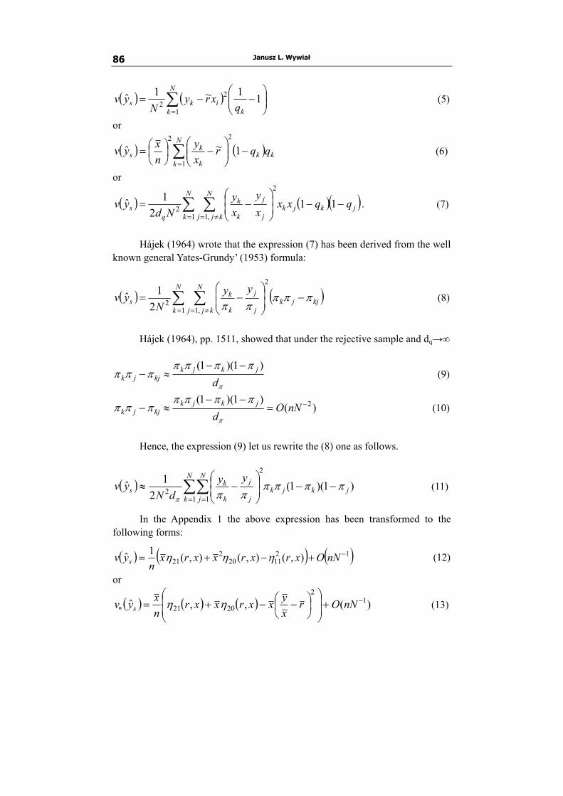
Janusz L. Wywiał 86
( ) ( )∑=
⎟⎟⎠
⎞⎜⎜⎝
⎛−−=
N
k kiks q
xryN
yv1
22 11~1ˆ (5)
or
( ) ( )∑=
−⎟⎟⎠
⎞⎜⎜⎝
⎛−⎟
⎠⎞
⎜⎝⎛=
N
kkk
k
ks qqr
xy
nxyv
1
22
1~ˆ (6)
or
( ) ( )( )∑ ∑= ≠=
−−⎟⎟⎠
⎞⎜⎜⎝
⎛−=
N
kjkjk
N
kjj j
j
k
k
qs qqxx
xy
xy
Ndyv
1 ,1
2
2 112
1ˆ . (7)
Hájek (1964) wrote that the expression (7) has been derived from the well known general Yates-Grundy’ (1953) formula:
( ) ( )∑ ∑= ≠=
−⎟⎟⎠
⎞⎜⎜⎝
⎛−=
N
kkjjk
N
kjj j
j
k
ks
yyN
yv1 ,1
2
221ˆ πππ
ππ (8)
Hájek (1964), pp. 1511, showed that under the rejective sample and dq→∞
π
πππππππ
djkjk
kjjk)1)(1( −−
≈− (9)
)()1)(1( 2−=
−−≈− nNO
djkjk
kjjkπ
πππππππ (10)
Hence, the expression (9) let us rewrite the (8) one as follows.
( ) ∑∑= =
−−⎟⎟⎠
⎞⎜⎜⎝
⎛−≈
N
kjkjk
N
j j
j
k
ks
yydN
yv1 1
2
2 )1)(1(2
1ˆ πππππππ
(11)
In the Appendix 1 the above expression has been transformed to the following forms:
( ) ( ) ( )121120
221 ),(),(),(1ˆ −+−+= nNOxrxrxxrx
nyv s ηηη (12)
or
( ) ( ) ( ) )(,,ˆ 12
2021−
∗ +⎟⎟⎠
⎞⎜⎜⎝
⎛⎟⎠⎞
⎜⎝⎛ −−+= nNOr
xyxxrxxr
nxyv s ηη (13)

ON LIMIT DISTRIBUTION OF HORVITZ-THOMPSON STATISTIC… 87
because ( ) xryxr −=,11η . The equality 0=− rxy
is possible when the joint
distribution of the variable under study and the auxiliary one is symmetric. ( ) =syv ˆ*
( ) ( ) ( ) ( )( ) ( ) +⎟⎟⎠
⎞⎜⎜⎝
⎛⎟⎠⎞
⎜⎝⎛ −−+−=
2
20220402021 ,,,,, r
xyxxrxxrxrxrxr
nx ηηηητ
)( 1−+ nNO (14) where the symbols γx, ηut(.,.), are explained at the beginning of the paper and
( ) ( )( ) ( ) ( )( ) ,
,,,
,,2204020
2121
xrxrxr
xrxrηηη
ητ−
= ( ) 1,1 21 ≤≤− xrτ .
4. Variance of the Horvitz-Thompson estimator
under existing measuring errors
Let us assume that values of the variable y have to be measured. The
values of the variable x are observations of y which can be biased by measuring error. The measure errors are denoted by ek, k∈U, and the first additive model of generating the values of the variable x is as follows.
xk = yk+ek, k = 1,…,N.
or equivalently by
yk = xk-ek, k = 1,…,N and the expression (13) takes the following form
( ) ( ) ( ) )(,,ˆ 12
22021
−∗ +⎟
⎟⎠
⎞⎜⎜⎝
⎛⎟⎠⎞
⎜⎝⎛ −−+= nNOh
xexxhxxh
nxyv s ηη
where ∑∈
=Uk
khN
h 1 and
k
kk x
eh = is the relative measuring error and it is
treated as the value of the variable h.

Janusz L. Wywiał 88
The next model of generating the values of the variable x is multiplicative and it is defined by
k
kk c
yx = , k=1,…,N
or equivalently by
yk=xkck, k=1,…,N
Now, the expression (13) takes the following form
( ) ( ) ( ) )(,,ˆ 12
22021*
−+⎟⎟⎠
⎞⎜⎜⎝
⎛⎟⎠⎞
⎜⎝⎛ −−+= nNOc
xyxxcxxc
nxyv s ηη
5. Estimators of the variance
Hájek (1964), pp. 1520, proposed to estimate the variance ( )syv ˆ by means of the following statistics
( ) ( )∑=
−⎟⎟⎠
⎞⎜⎜⎝
⎛−
−=
N
kkks
k
kss aqr
xy
nnxyv
1
221~
)1(ˆ (15)
where
( )
( )∑
∑
=
=
−
−= N
kkk
N
kkk
k
k
s
aq
aqxy
r
1
1
1
1~ . (16)
The well known Groudy and Yates estimator of the variance is as follows:
( ) kj
N
k kj
kjjkN
kjj j
j
k
kss aa
yyN
yv ∑ ∑= ≠=
−⎟⎟⎠
⎞⎜⎜⎝
⎛−=
1 ,1
2
221ˆ
ππππ
ππ (17)
where πk= qk, k=1,…,N.

ON LIMIT DISTRIBUTION OF HORVITZ-THOMPSON STATISTIC… 89
On the basis of the expression (9) we have
( ))1)(1(1
jkjkkj dd
πππππ π
π
−−−≈
and
)1)(1()1)(1(
jk
jk
kj
kjjk
d ππππ
ππππ
π −−−−−
≈−
. (18)
The above results let us transform the expression (17) to the form:
( ) kj
N
k jk
jkN
kjj j
j
k
kss aa
dyy
Nyv ∑ ∑
= ≠= −−−−−
⎟⎟⎠
⎞⎜⎜⎝
⎛−=
1 ,1
2
2 )1)(1()1)(1(
21ˆˆ
ππππ
ππ π (19)
So, ( )( ) ( )sss yvyvE ˆˆˆ = , when dπ→∞.
Theorem 1. Let the mean value of the auxiliary variable fulfil the inequalities Mxxx ≤≤0 , v02<∞, v20<∞, v40<∞. Under the rejective sampling design for qk, k=1,..,N, given by the expression (1) the statistic ( )ss yv ˆˆ is the design consistent estimator of the variance ( )syv ˆ , when dπ→∞.
The proof is included in the appendix 2. 6. Limit distribution
Hájek (1964), pp. 1514-5, proved the following (see Berger (1992), too). Theorem 2. If the rejective sampling design is implemented the statistic
( )s
ss yv
yytˆ
ˆ −=
has the standard normal distribution, so )1,0(~ Ntts → , if and only if dq→∞ and ξ→0, where ξ = {ε: L(ε)},≤ε},
( ) ( ){ }∑
>
−=
skk yvqzk k
kk
s qqz
yvL
ˆ:
2 1ˆ1)(
ε
ε ,
Janusz L. Wywiał 90
kkk xryz ~−= and r~ is defined by the expression (4).
We are going to prove the similar theorem but about convergence to normality of the statistics:
( )ss
ss yv
yytˆˆ
ˆˆ −= (20)
where the sample variance ( )ss yv ˆˆ is defined by the expression (19).
Theorem 3. Let the mean value of the auxiliary variable fulfil the inequalities Mxxx ≤≤0 , v02<∞, v20<∞, v40<∞. Under the rejective sampling design for qk, k = 1,..,N, given by the expression (1) the statistic
)1,0(~ˆ Nts , when n→∞ and N-n→∞. Moreover, under the additional
assumption that 0=− rxy
, )1,0(~ Nt s∗ .
Proof. The theorem results straightforward from the theorems 1 and 2 and
from the well known theorem of Sludzki, see Berger and Skinner (2005), too.
7. Conclusion
Asymptotic normality of the Horvitz-Thompson statistic is very important
from practical point of view because it let us construct confidence interval for the population mean as well as testing statistical hypothesis on mean value. For instance, such hypotheses are considered in financial audit, because there is frequently considered rejecting sampling design as a particular case of so called dollar sampling. Acknowledgement
The research was supported by the grant number N N111 434137 from the Polish Ministry of Science and Higher Education.
Appendix 1
The derivation of the expression (12).

ON LIMIT DISTRIBUTION OF HORVITZ-THOMPSON STATISTIC… 91
( ) =−−⎟⎟⎠
⎞⎜⎜⎝
⎛−≈ ∑∑
= =
N
kjkjk
N
j j
j
k
ks x
yxy
dnxyv
1 1
2
2
2)1)(1(
2ˆ ππππ
π
( ) ( )( ) =−−−−−= ∑∑= =
N
kjkjk
N
jjk rrrr
dnx
1 1
22
2)1)(1(
2ππππ
π
( ) ( )( )( ) =−−−−−−= ∑∑= =
N
kjkjk
N
jjkk rrrrrr
dnx
1 1
22
2)1)(1(22
2ππππ
π
( ) −−−−= ∑∑= =
N
kjkjk
N
jk rr
dnx
1 1
22
2)1)(1( ππππ
π
( )( ) =−−−−− ∑∑= =
N
kjkjk
N
jjk rrrr
dnx
1 12
2)1)(1( ππππ
π
( ) ( ) =⎟⎟
⎠
⎞
⎜⎜
⎝
⎛⎟⎟⎠
⎞⎜⎜⎝
⎛−−−−−−= ∑∑∑
===
2
111
22
2)1()1()1( kk
N
kk
N
jjjkk
N
kk rrrr
dnx ππππππ
π
So,
( ) ( ) ( )2
13
2
1
22
2)1()1(ˆ ⎟⎟⎠
⎞⎜⎜⎝
⎛−−−−−= ∑∑
==kk
N
kkkk
N
kks rr
nxrr
nxyv ππππ (21)
( ) ( ) =⎟⎠⎞
⎜⎝⎛ −−=−− ∑∑
==kk
N
kkkk
N
kk x
nxNxrr
xNnrr
122
2
1)1( ππ
( ) ( )( ) ( ) =⎟⎟⎠
⎞⎜⎜⎝
⎛−−⎟
⎠⎞
⎜⎝⎛ −+−−= ∑
=
xxxnNxxxrr
xNn
kk
N
kk 1
122
2
( ) )(),(),(2),(),( 121111122
2
11−+=−+= NnOxr
xnxrxxr
xNnxr
xn ηηηη (22)
Next, we have:

Janusz L. Wywiał 92
( ) =−−∑=
)1(1
2kk
N
kk rr ππ
( ) ( ) ( ) =⎟⎟⎠
⎞⎜⎜⎝
⎛⎟⎠⎞
⎜⎝⎛ −+−−−⎟
⎠⎞
⎜⎝⎛ −−= ∑
=
22
1
222
212 x
nNxxxxx
nNrr
xNn
kk
N
kk
=⎟⎟⎠
⎞⎜⎜⎝
⎛⎟⎠⎞
⎜⎝⎛ −+−⎟
⎠⎞
⎜⎝⎛ −= ),(1),(),(2 20
222212
2xrx
nNxrxrx
nN
xNn ηηη
( ) ( )=++−+= ),(),(),(),(),( 202
21222
2
2021 xrxxrxxrxN
nxrxxrxn ηηηηη
( ) ( )122021 ),(),( −−+= NnOxrxxr
xn ηη
Finnaly, the obtained result and the results (22) and (21) lead to the
expression (12). Appendix 2
Proof of the theorem 1. Hájek (1964), pp. 1508, proved that for all k = 1,…,N, qk→πk when d→∞, where d is given by the equation (3).
Let us remind ourself the following definition the symbol O(.) explained e.g. by Leja (1977).
Definiton 1. Let h(u) and t(u) be two functions defined in a neighbourhood of value u0. The symbol O(t) means that there exists such the neighbourhood 0<|u-u0|<δ and the value M that
Mutuh
≤)()(
The Definition 1 and the expression (1) lead to the following. Let
xNxgNh k
k ==)( and t(N)=N-1. Now, we have

ON LIMIT DISTRIBUTION OF HORVITZ-THOMPSON STATISTIC… 93
∞<=≤= Mxx
xx
NtNh M
k 0)()(
, k = 1,…,N.
So, gk = O(N-1) because the above inequality is true for all N>0. ( ) ( )( ) ( ) ( )( )( ) ( )( ) ==−=− sssssssss yvVyvEyvEyvyvE ˆˆˆˆˆˆˆˆˆ 22
( )( ) ( )sss yvyvE ˆˆˆ 22 −=
( )( ) ( ) +⎜⎜⎜
⎝
⎛
−−−
−−⎟⎟⎠
⎞⎜⎜⎝
⎛−= ∑ ∑
= ≠=
N
kkj
jk
jkN
kjj j
j
k
kss d
yyN
yvE1
2
22
,1
4
42
)1)(1()1()1(
21ˆˆ π
ππππ
ππ π
⋅⎟⎟⎠
⎞⎜⎜⎝
⎛−⎟
⎟⎠
⎞⎜⎜⎝
⎛−+∑∑∑∑
= = = =
N
k
N
j
N
i
N
h h
h
i
i
j
j
k
k yyyy
1 1 1 1
22
ππππ
( ) ( ) ( )⎟⎟⎠
⎞
−−−−−
−−−
−−⋅ hijk
hi
hi
jk
jk aaaaEdd )1)(1(
)1)(1()1)(1(
)1)(1(ππ
ππππ
ππ
ππ
It is well known that
( ) ( ) ( ) ( ) ( ) ilkjlijklijkljik aaEaaEaaEaaEaaaaE ππ==≤ 22
( )( ) ( ) +⎜⎜⎜
⎝
⎛
−−−
−−⎟⎟⎠
⎞⎜⎜⎝
⎛−≤ ∑ ∑
= ≠=
N
kkj
jk
jkN
kjj j
j
k
kss d
yyN
yvE1
2
22
,1
4
42
)1)(1()1()1(
21ˆˆ π
ππππ
ππ π
⋅⎟⎟⎠
⎞⎜⎜⎝
⎛−⎟
⎟⎠
⎞⎜⎜⎝
⎛−+∑∑∑∑
= = = =
N
k
N
j
N
i
N
h h
h
i
i
j
j
k
k yyyy
1 1 1 1
22
ππππ
( ) ( ) ≈⎟⎟⎠
⎞
−−−−−
−−−
−−⋅ ihkj
hi
hi
jk
jk
ddππ
ππππ
ππππ
ππ )1)(1()1)(1(
)1)(1()1)(1(

Janusz L. Wywiał 94
( ) +⎜⎜⎜
⎝
⎛
−−−−−
⎟⎟⎠
⎞⎜⎜⎝
⎛−≈ ∑ ∑
= ≠=
N
k jk
jkjkN
kjj j
j
k
k
ddyy
N 1
22
,1
4
4 )1)(1()1()1(
21
ππ ππππππ
ππ
( )( ) =⎟⎟⎟
⎠
⎞−−⎟⎟
⎠
⎞⎜⎜⎝
⎛−⎟
⎟⎠
⎞⎜⎜⎝
⎛−+∑∑∑∑
= = = =ihhikjjk
N
k
N
j
N
i
N
h h
h
i
i
j
j
k
k yyyy ππππππππππ1 1 1 1
22
( ) +−−−
−−⎟⎟⎠
⎞⎜⎜⎝
⎛−≈ ∑ ∑
= ≠=
N
k jk
jkjkN
kjj j
j
k
k
ddyy
N 1
22
,1
4
4 )1)(1()1()1(
21
ππ ππππππ
ππ
( )( ) =⎟⎟⎟
⎠
⎞−−⎟⎟
⎠
⎞⎜⎜⎝
⎛−⎟
⎟⎠
⎞⎜⎜⎝
⎛−+∑∑∑∑
= = = =ihhikjjk
N
k
N
j
N
i
N
h h
h
i
i
j
j
k
k yyyy ππππππππππ1 1 1 1
22
( ) +−−−
−−⎟⎟⎠
⎞⎜⎜⎝
⎛−= ∑ ∑
= ≠=
N
k jk
jkjkN
kjj j
j
k
k
ddyy
N 1
22
,1
4
4 )1)(1()1()1(
21
ππ ππππππ
ππ
( )⎟⎟⎟
⎠
⎞
⎟⎟⎟
⎠
⎞
⎜⎜⎜
⎝
⎛−⎟
⎟⎠
⎞⎜⎜⎝
⎛−+ ∑∑∑∑
= = = =
2
1 1 1 1
2
kjjk
N
k
N
j
N
i
N
h j
j
k
k yy πππππ
Hence,
( )( ) ( ) ( )s
N
k jk
jkjkN
kjj j
j
k
kss yv
ddyy
NyvE ˆ
)1)(1()1()1(
21ˆˆ 2
1
22
,1
4
42 +
−−−−−
⎟⎟⎠
⎞⎜⎜⎝
⎛−≤ ∑ ∑
= ≠= ππ ππππππ
ππ
( ) ( )( ) ( )∑ ∑= ≠= −−−
−−⎟⎟⎠
⎞⎜⎜⎝
⎛−≤−
N
k jk
jkjkN
kjj j
j
k
ksss dd
yyN
yvyvE1
22
,1
4
42
)1)(1()1()1(
21ˆˆˆ
ππ ππππππ
ππ
( ) ( ) ( ) ( )∑ ∑=
−−
≠=
− =−=N
k
N
kjjjk NnOnOyynNO
N 1
222
,1
44442
1

ON LIMIT DISTRIBUTION OF HORVITZ-THOMPSON STATISTIC… 95
( ) ( ) ( )( )20240
4
1 ,1
442 2221 vvnOyynNO
N
k
N
kjjjk +=−= −
= ≠=
−− ∑ ∑ .
So,
( ) ( )( ) ( )42ˆˆˆ −≤− nOyvyvE sss Hence, on the basis of the well known Tchebyshev inequality we have:
( ) ( )( ) ( )( )
( )( )( ) ( )2
2 ˆˆˆ
1ˆˆˆˆˆˆ0 −=≤⎟
⎟⎠
⎞⎜⎜⎝
⎛≥−=≤−≤ nO
yvyvV
yvyvPyvyvP
s
ss
s
sssss δ
δς .
So, the estimator ( )ss yv ˆˆ converges to the variance ( )syv ˆ when n→∞ and
N-n→∞. References Berger, Y.G. (1998) Rate of convergence to normal distribution for Horvitz-
Thompson estimator. “Journal of Statistical Planning and Inference” 67, 209-226.
Berger, Y.G., Skinner, C.J. (2005) A jackknife variance estimator for unequal probability sampling. “Journal of the Royal Statistical Society” B 67, 79-89.
Hájek, J. (1964) Asymptotic theory of rejective sampling with varying probabilities from a finite population. “Annals of Mathematical Statistics” 35, 1491-1523.
Horvitz, D.G., Thompson, D.J. (1952) A generalization of sampling without replacement from finite universe. “Journal of the American Statistical Association” Vol. 47, 663-685.
Leja, F. (1977) Difference and Integral Calculus (in Polish). PWN, Warszawa.
Tillé, Y. (2006) Sampling Algorithms. Springer.
Yates, F., Grundy, P.M. (1953) Selection without replacement from within strata with probability proportional to size. “Journal of the Royal Statistical Society”, Series B, 15: 235-261.

Janusz L. Wywiał 96
O ROZKŁADZIE GRANICZNYM STATYSTYKI HORVITZA-THOMPSONA Z PRÓBY DOBIERANEJ
ZA POMOCĄ SCHEMATU LOSOWANIA ZWROTNEGO ODRZUCAJĄCEGO PRÓBY Z POWTÓRZENIAMI ELEMENTÓW
Streszczenie
Rozważany jest problem wnioskowania o wartości przeciętnej w po-pulacji skończonej i ustalonej na podstawie próby, do której są losowane elementy populacji z prawdopodobieństwami proporcjonalnymi do wartości cechy dodatkowej. Losowanie zwrotne próby o zadanej z góry liczebności jest powtarzane tak długo, aż uzyskamy taką, w której elementy populacji nie powtarzają się. Hajek wykazał, że statystyka Horvitza-Thompsona dla obserwacji zmiennej w tak losowanej próbie ma granicznie rozkład normalny m.in. pod warunkami, że rozmiary próby i populacji wzrastają w sposób nieograniczony oraz wariancja statystyki Horvitza-Thompsona jest znana. Treść niniejszej pracy jest nieznacznym uogólnieniem tej własności granicznej rozkładu prawdopodobieństwa statystyki Horvitza-Thompsona na przypa- dek, gdy jej wariancja jest oceniania za pomocą znanego estymatora Yatesa i Grundy’ego.

Tomasz Żądło
ON ACCURACY OF TWO PREDICTORS
FOR SPATIALLY AND TEMPORALLY
CORRELATED LONGITUDINAL DATA
1. Basic notations
Longitudinal data for periods t = 1,...,M are considered. In the period t the population of size tN is denoted by tΩ . The population in the period t is divided
into D disjoint subpopulations (domains) dtΩ of size dtN , where d = 1,...,D. Let the set of population elements for which observations are available in the period t be denoted by st and its size by nt. The set of subpopulation elements for which observations are available in the period t is denoted by dts and its size by ndt.
Let: rdt dt dtsΩ = Ω − , rdt dt dtN N n= − .
Let idM denotes the number of periods when the i-th population element belongs to the d-th domain. Let us denote the number of periods when the i-th population element (which belongs to the d-th domain) is observed by idm . Let
rid id idm M m= − . It is assumed that the population may change in time and that one population element may change its domain affiliation in time (from technical point of view observations of some population element which change its domain affiliation are treated as observations of new population element). It means that i and t completely identify domain affiliation but additional subscript d will be needed as well. More about this assumptions will be written at the end of the next section.
The set of elements which belong at least in one of periods t = 1,...,M to sets tΩ is denoted by Ω and its size by N. Similarly, sets dΩ , s , ds , rdΩ of
sizes dN , n, dn , rdN respectively are defined as sets of elements which belong
at least in one of periods t = 1,...,M to sets dtΩ , ts , dts , rdtΩ respectively. The
d*-th domain of interest in the period of interest t* will be denoted by * *d tΩ , and
Tomasz Żądło 98
the set of elements which belong at least in one of periods t = 1,...,M to sets
* *d tΩ will be denoted by *dΩ . The introduced notations allow to assume that the domain affiliations of
population elements change in time.
2. First predictor
Superpopulation models used for longitudinal data (compare Verbeke and Molenberghs, 2000; Hedeker and Gibbons, 2006) are considered which are – what is important for further considerations – special cases of the General Linear Model (GLM) and the General Linear Mixed Model (GLMM). We propose the following model:
= + +d d d d d dY X β Z v e , (1)
where 1
( )di N
col≤ ≤
=d idY Y , where idY is a random vector, called profile, of size
1idM × , and dY (d = 1,...,D) are assumed to be independent,
1( )
di Ncol
≤ ≤=d idX X , where idX is known matrix of size idM p× ,
1( )
di Ndiag
≤ ≤=d idZ Z , where idZ is known vector of size 1idM × ,
1( )
didi N
col v≤ ≤
=dv , where idv is a profile-specific random component and dv
(d = 1,2...,D) are assumed to be independent, 1
( )di N
col≤ ≤
=d ide e , where ide is
a random component vector of size 1idM × and ide ( i = 1,...,N; d = 1,...,D) are
assumed to be independent, dv and de are assumed to be independent.
What is more, it is assumed that vector of random components dv obey assumptions of simultaneously spatial autoregressive (SAR) process:
( )sp dρ= +d d dv W v u , (2)
where dW is the spatial weight matrix for profiles idY , 2~ ( , )d
u Nσdu 0 I .
Hence,
( )~ ,d dv 0 R , (3)
where 2uσ=
-1d dR C
and ( )( )( ) ( )
dsp spN
ρ ρ= − −d
Td d dN
C I W I W .
Moreover, elements of ide obey assumptions of autoregressive process AR(1):
( ) 1idj t idj idje eρ ε−= + . (4)
Hence,

ON ACCURACY OF TWO PREDICTORS FOR SPATIALLY… 99
( )~ ,eid id0 Σ , (5)
where elements of idΣ are given by ( ) 12 2( ) ( )1k lt tεσ ρ ρ
−− − .
Under the model, based on the theorem presented by Royall (1976), the best linear unbiased predictor is given by:
* *
(1)* * * *
ˆ ˆd t
BLUd t id t
i sYθ
∈
= + +∑ rd*t* d*x β%
( ) ( )*
2 1* * * * * * *1
ˆ( )rd
u i Ndiagσ −
≤ ≤+ + −T -1 T
rd* rd d sd rs id ss d sd sd d*γ Z C Z Σ V Y X β , (6)
where rd*t*x% is a 1 p× vector of totals of auxiliary variables in * *rd tΩ ,
( ) 1
* * * * * *ˆ −
= T -1 T -1d* sd ss d sd sd ss d sdβ X V X X V Y ,
( )*
11 2
* * * * *1( )
d
Tu i n
diagσ−
−≤ ≤
= +-1ss d sd d sd ss idV Z C Z Σ , *sdX is known
*
*1
dn
idi
m p=
×∑
matrix of auxiliary variables, *sdY is a *
*1
1dn
idi
m=
×∑ vector of random variables
idjY , rd*γ is a *
*1
1dn
ridi
M=
×∑ vector of one’s for observations in period *t
(in * *rd tΩ ) and zero otherwise, sdZ and rdZ are submatrices of dZ obtained
by deleting rows for unsampled and sampled elements respectively, ss idΣ is
a submatrix obtained from idΣ by deleting rows and columns for unsampled
observations., where rs idΣ is a submatrix obtained from idΣ by deleting rows
for sampled observations and columns for unsampled observations. 3. Second predictor
Let us assume model (1) with (2) and (4) where ( ) 0spρ = and ( ) 0tρ =
what means that elements of de and elements dv are uncorrelated. Based on the model predictor (6) simplifies to the formula (see Żądło 2011):
* * * * *
* * * * * * * * *
* *
2 1
1 1
2)*
1
(*
ˆ ˆ( ),ˆ rd t rd t id
d t
N N m
vid t id id ji s i i
BLUd t
jY b Yθ σ −
∈ = = =
= + + −∑ ∑ ∑ ∑id t d id j dx β x β (7)

Tomasz Żądło 100
where * *2 2e vid id
b mσ σ= + , 1 2 ...idj idj idjpx x x⎡ ⎤= ⎣ ⎦idjx
* *
* * * * * * *
1
1 1
1 1
ˆ d dn n
id idi i
b b−
− −
= =
⎛ ⎞ ⎛ ⎞= ⎜ ⎟ ⎜ ⎟⎜ ⎟ ⎜ ⎟⎝ ⎠ ⎝ ⎠∑ ∑T T
d sid sid sid sidYβ X X X and *sid
X is *idm p× known
matrix of auxiliary variables. 4. Simulation study
Limited model-based simulation study prepared using R (R Development Core Team 2011) is based on artificial data. Population of size N = 200 elements is divided into D = 10 domains of sizes {15, 15, 15, 20, 20, 20, 20, 25, 25, 25}. Number of periods M = 3 and balanced panel sample is studied – in each period the same 5dn = elements from each domain are observed in the sample (overall sample size in each period is n = 50). The purpose of the study is to predict D = 10 domain totals for the last period. Data are generated based on model (1) where 1idj idjx∀ = , 1idj idjz∀ = ,
d dβ β∀ = and for arbitrary chosen values of parameters 100β = , 2 1εσ = , 2 1uσ = . For these assumptions and balanced panel sample predictor (7)
simplifies to (Żądło (2010)):
*
* * *ˆ ˆ
d t
BLU id t rd ti s
Y Nθ μ∈
= +∑ (8)
where 1 1
1 1 1
ˆdnD m
idjd i j
n m Yμ − −
= = =
= ∑∑∑ .
In the simulation the following predictors are considered:
– predictor given by (6) assuming that variance-covariance parameters are known, denoted by BLUP,
– predictor given by (6) where variance-covariance parameters are estimated using Restricted Maximum Likelihood Estimators, denoted by EBLUP,
– predictor given by (8), denoted by SIMPLE. In the simulation the following values of ( )spρ and ( )tρ are considered:
0,8; 0,3; -0,3 and -0,8 what gives sixteen pairs of these correlation coefficients (these pairs are presented on x-axis). Realizations of random components are generated using multivariate normal distribution. The following three graphs allow to compare MSEs of the considered predictors.

ON ACCURACY OF TWO PREDICTORS FOR SPATIALLY… 101
(.8,.8) (.8,.3) (.8,-.3) (.8,-.8) (.3,.8) (.3,.3) (.3,-.3) (.3,-.8) (-.3,.8) (-.3,.3) (-.3,-.3) (-.3,-.8) (-.8,.8) (-.8,.3) (-.8,-.3) (-.8,-.8)
1.00
1.02
1.04
1.06
1.08
1.10
1.12
Graph 1. Values of MSE(EBLUP)/MSE(BLUP)
(.8,.8) (.8,.3) (.8,-.3) (.8,-.8) (.3,.8) (.3,.3) (.3,-.3) (.3,-.8) (-.3,.8) (-.3,.3) (-.3,-.3) (-.3,-.8) (-.8,.8) (-.8,.3) (-.8,-.3) (-.8,-.8)
1.00
1.05
1.10
1.15
1.20
1.25
1.30
Graph 2. Values of MSE(SIMPLE)/MSE(BLUP)
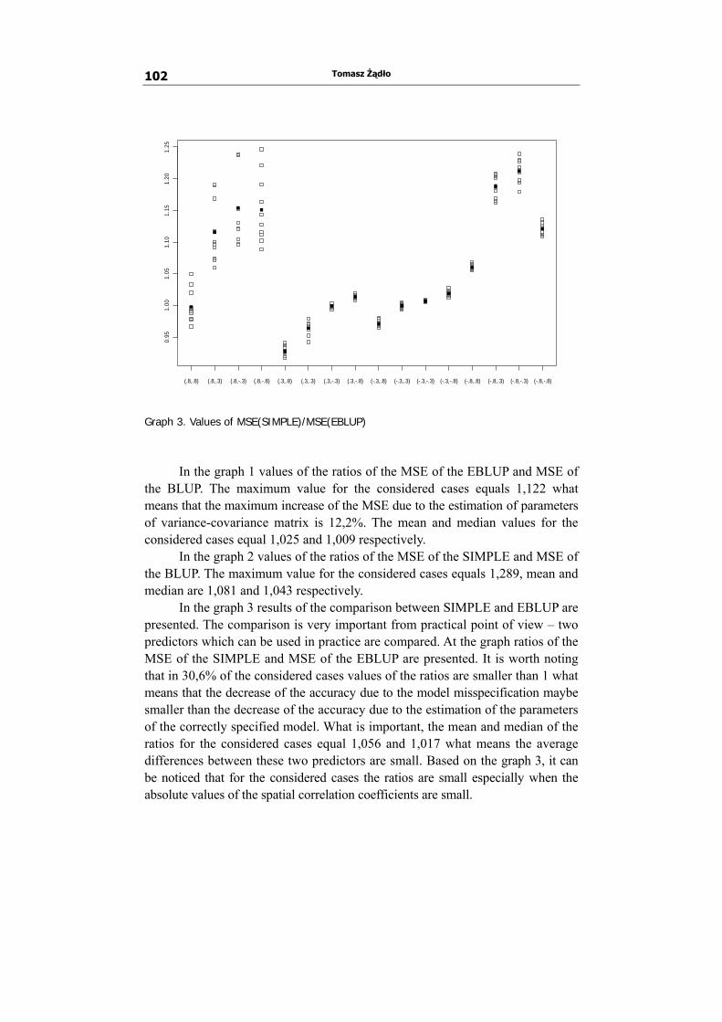
Tomasz Żądło 102
(.8,.8) (.8,.3) (.8,-.3) (.8,-.8) (.3,.8) (.3,.3) (.3,-.3) (.3,-.8) (-.3,.8) (-.3,.3) (-.3,-.3) (-.3,-.8) (-.8,.8) (-.8,.3) (-.8,-.3) (-.8,-.8)
0.95
1.00
1.05
1.10
1.15
1.20
1.25
Graph 3. Values of MSE(SIMPLE)/MSE(EBLUP)
In the graph 1 values of the ratios of the MSE of the EBLUP and MSE of the BLUP. The maximum value for the considered cases equals 1,122 what means that the maximum increase of the MSE due to the estimation of parameters of variance-covariance matrix is 12,2%. The mean and median values for the considered cases equal 1,025 and 1,009 respectively. In the graph 2 values of the ratios of the MSE of the SIMPLE and MSE of the BLUP. The maximum value for the considered cases equals 1,289, mean and median are 1,081 and 1,043 respectively. In the graph 3 results of the comparison between SIMPLE and EBLUP are presented. The comparison is very important from practical point of view – two predictors which can be used in practice are compared. At the graph ratios of the MSE of the SIMPLE and MSE of the EBLUP are presented. It is worth noting that in 30,6% of the considered cases values of the ratios are smaller than 1 what means that the decrease of the accuracy due to the model misspecification maybe smaller than the decrease of the accuracy due to the estimation of the parameters of the correctly specified model. What is important, the mean and median of the ratios for the considered cases equal 1,056 and 1,017 what means the average differences between these two predictors are small. Based on the graph 3, it can be noticed that for the considered cases the ratios are small especially when the absolute values of the spatial correlation coefficients are small.
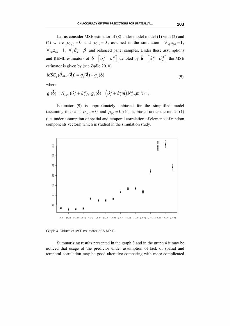
ON ACCURACY OF TWO PREDICTORS FOR SPATIALLY… 103
Let us consider MSE estimator of (8) under model model (1) with (2) and (4) where ( ) 0spρ = and ( ) 0tρ = , assumed in the simulation 1idj idjx∀ = ,
1idj idjz∀ = , d dβ β∀ = and balanced panel samples. Under these assumptions
and REML estimators of 2 2e uσ σ⎡ ⎤= ⎣ ⎦δ denoted by 2 2ˆ ˆˆ
e uσ σ⎡ ⎤= ⎣ ⎦δ the MSE
estimator is given by (see Żądło 2010)
$1 2
ˆ ˆ( )) ˆ ˆ( ( ) ( )BLUMSE g gξ θ += δ δδ (9) where
2 21 *
ˆ ˆ ˆ( ) ( )rd t e vg N σ σ= +δ , ( )2 2 12 12 *ˆˆ ˆ( ) v rd teg m N m nσ σ − −= +δ ,
Estimator (9) is approximately unbiased for the simplified model (assuming inter alia ( ) 0spρ = and ( ) 0tρ = ) but is biased under the model (1)
(i.e. under assumption of spatial and temporal correlation of elements of random components vectors) which is studied in the simulation study.
(.8,.8) (.8,.3) (.8,-.3) (.8,-.8) (.3,.8) (.3,.3) (.3,-.3) (.3,-.8) (-.3,.8) (-.3,.3) (-.3,-.3) (-.3,-.8) (-.8,.8) (-.8,.3) (-.8,-.3) (-.8,-.8)
-50
050
100
150
200
250
Graph 4. Values of MSE estimator of SIMPLE
Summarizing results presented in the graph 3 and in the graph 4 it may be noticed that usage of the predictor under assumption of lack of spatial and temporal correlation may be good alterative comparing with more complicated

Tomasz Żądło 104
predictor under assumption of nonzero spatial and temporal correlation. But in this case correct estimator of MSE should be used. 5. Summary
Based on the simulation study two predictors were compared for spatially and temporally correlated longitudinal data. The first one under the correctly specified model where unknown parameters are estimated using REML and the second predictor under the misspecified model (under assumption of the lack of spatial and temporal correlation). It was shown, especially for small values of spatial correlation, that the second, simpler predictor can be a good alternative to the first one. References Chandra, H., Salvati, N., Chambers, R. (2007) Small area estimation for
spatially correlated populations – a comparison of direct and indirect model-based methods. “Statistics in Transition” 8(2), 331-350.
Hedeker, D., Gibbons, R.D. (2006) Longitudinal Data Analysis. John Wiley and Sons, New Jersey.
Henderson, C.R. (1950) Estimation of genetic parameters (Abstract). “Annals of Mathematical Statistics” 21, 309-310.
Molina, I., Salvati, N., Pratesi, M. (2009) Bootstrap for estimating the MSE of the Spatial EBLUP. “Computational Statistics” 24, 441-458.
Petrucci, A., Salvati, N. (2006) Small area estimation for spatial correlation in watershed erosion assessment. “J Agric Biol Environ Stat” 11, 169-182.
Pratesi, M., Salvati, N. (2008) Small area estimation: the EBLUP estimator based on spatially correlated random area effects. “Stat Methods Appl” 17, 113-141.
Petrucci, A., Pratesi, M., Salvati, N. (2005) Geographic information in small area estimation: small area models and spatially correlated random area effects. “Statistics in Transition” 7(3), 609-623.
Rao, J.N.K (2003) Small area estimation. John Wiley and Sons, New Jersey.
Rao, J.N.K, Yu, M. (1994) Small-Area Estimation by Combining Time-Series and Cross-Sectional Data. “The Canadian Journal of Statistics” 22(4), 511-528.

ON ACCURACY OF TWO PREDICTORS FOR SPATIALLY… 105
R Development Core Team (2011) A language and environment for statistical computing. R Foundation for Statistical Computing, Vienna.
Royall, R.M. (1976) The linear least squares prediction approach to two- stage sampling. JASA, 71, 657-664.
Salvati, N., Pratesi, M., Tzavidis, N., Chambers, R. (2009) Spatial M-quantile models for small area estimation. “Statistics in Transition” 10(2), 251- -261.
Saei, A., Chambers, R. (2003) Small area estimation under linear and generalized linear mixed models with time an area effects. “S3RI Methodology Working Paper” M03/15r, University of Southampton.
Verbeke, G., Molenberghs, G.(2000) Linear Mixed Models for Longitudinal Data. Springer-Verlag, New York.
Żadło, T. (2010) On prediction of domain total based on balanced panel data. Acta Universitatis Lodziensis, Folia Oeconomica 235, 63-72.
Żądło, T. (2011) On some problems of prediction of domain total in longitudinal surveys when auxiliary information is available, submitted to Studia Ekonomiczne.
O DOKŁADNOŚCI DWÓCH PREDYKTORÓW DLA SKORELOWANYCH DANYCH
PRZEKROJOWO-CZASOWYCH
Streszczenie
Rozważny jest model dla danych przekrojowo-czasowych uwzględniający dwa składniki losowe spełniające odpowiednio założenia przestrzennego modelu autoregresyjnego oraz modelu autoregresyjnego w czasie. W pracy rozważane są dwa predyktory wartości globalnej w domenie. Pierwszy z nich jest empirycz-nym najlepszym liniowym nieobciążonym predyktorem wyprowadzonym przy założeniu wspomnianego modelu. Drugi jest najlepszym liniowym nieobcią-żonym predyktorem przy założeniu modelu mieszanego, w którym elementy składników losowych są niezależne. Analiza została wsparta badaniami symula-cyjnymi.

AUTHORS Czesław Domański Department of Statistics Methods, University of Lodz, Poland Wojciech Gamrot Department of Statistics, Katowice University of Economics, Poland Janusz Gołaszewski Department of Plant Breeding and Seed Production, University of Warmia and Mazury in Olsztyn, Poland Anna Imiołek Department of Plant Breeding and Seed Production, University of Warmia and Mazury in Olsztyn, Poland Alina Jędrzejczak Centre for Mathematical Statistics, Statistical Office in Lodz Chair of Statistical Methods, Institute of Econometrics and Statistics, University of Lodz, Poland Arkadiusz Kozłowski Department of Statistics, University of Gdansk, Poland Jan Kubacki Centre for Mathematical Statistics, Statistical Office in Lodz, Poland Zbigniew Nasalski Department of Enterprise Economics, University of Warmia and Mazury in Olsztyn, Poland Dorota Raczkiewicz Institute of Statistics and Demography, Warsaw School of Economics, Poland Janusz L.Wywiał Department of Statistics, Katowice University of Economics, Poland Dariusz Załuski Department of Plant Breeding and Seed Production, University of Warmia and Mazury in Olsztyn, Poland Tomasz Żądło Department of Statistics, Katowice University of Economics, Poland Ondřej Vilikus University of Economics, Prague, Czech Republic