1

Genome-wide signatures of population bottlenecks and 1

diversifying selection in European wolves 2

3

M Pilot1,2

, C Greco3, BM vonHoldt

4, B Jędrzejewska

5, E Randi

3, 6, 4

W Jędrzejewski5, 9

, VE Sidorovich7, EA Ostrander

8, RK Wayne

4 5

6

1School of Life Sciences, University of Lincoln, Brayford Pool, Lincoln 7

LN6 7TS, UK; 8

2Museum and Institute of Zoology, Polish Academy of Sciences, Wilcza 64, 9

00-679 Warsaw, Poland; 10

3Istituto Superiore per la Protezione e la Ricerca Ambientale (ISPRA), 11

40064, Ozzano Emilia (BO), Italy; 12

4Department of Ecology and Evolutionary Biology, University of 13

California, Los Angeles, California 90095, USA; 14

5Mammal Research Institute, Polish Academy of Sciences, 17-230 15

Białowieża, Poland; 16

6Aalborg University, Department 18, Section of Environmental 17

Engineering, Aalborg, Denmark 18

7Institute of Zoology, National Academy of Sciences of Belarus, Minsk, 19

Belarus; 20

8Cancer Genetics Branch, National Human Genome Research Institute, 21

National Institutes of Health, Bethesda, Maryland 20892, USA; 22

9Present address: Instituto Venezolano de Investigaciones Cientificas 23

(IVIC), Centro de Ecologia, Caracas, Venezuela 24

2

Correspondence: RK Wayne, Department of Ecology and Evolutionary 25

Biology, University of California, Los Angeles, California 90095, USA. E-26

mail: rwayne@ucla.edu 27

28

Running title: Genome-wide diversification in European wolves 29

3

Abstract 30

Genomic resources developed for domesticated species provide powerful 31

tools for studying the evolutionary history of their wild relatives. Here we 32

use 61K single nucleotide polymorphisms (SNPs) evenly spaced throughout 33

the canine nuclear genome to analyse evolutionary relationships among 34

three largest European populations of grey wolves in comparison with other 35

populations worldwide, and investigate genome-wide effects of 36

demographic bottlenecks and signatures of selection. European wolves have 37

a discontinuous range, with large and connected populations in Eastern 38

Europe and relatively smaller, isolated populations in Italy and the Iberian 39

Peninsula. Our results suggest a continuous decline in wolf numbers in 40

Europe since the Late Pleistocene, and long-term isolation and bottlenecks 41

in the Italian and Iberian populations following their divergence from the 42

Eastern European population. The Italian and Iberian populations have low 43

genetic variability and high linkage disequilibrium, but relatively few 44

autozygous segments across the genome. This last characteristic clearly 45

distinguishes them from populations that underwent recent drastic 46

demographic declines or founder events, and implies long-term bottlenecks 47

in these two populations. Although genetic drift due to spatial isolation and 48

bottlenecks seems to be a major evolutionary force diversifying the 49

European populations, we detected 35 loci that are putatively under 50

diversifying selection. Two of these loci flank the canine platelet-derived 51

growth factor gene, which affects bone growth and may influence 52

differences in body size between wolf populations. This study demonstrates 53

4

the power of population genomics for identifying genetic signals of 54

demographic bottlenecks and detecting signatures of directional selection in 55

bottlenecked populations, despite their low background variability. 56

57

Keywords: bottleneck; effective population size; linkage disequilibrium; 58

genetic differentiation; selection; grey wolf59

5

INTRODUCTION 60

Studies on evolutionary processes in natural populations have been 61

greatly enabled by technological advances related to whole genome 62

sequence data from a variety of domesticated species (Allendorf et al. 63

2010). Access to large number of loci, often with annotated positions within 64

the genome of the investigated species, permits researchers to overcome 65

analytical limitations associated with the analysis of a small number of 66

genetic markers. Examples include reconstruction of admixture patterns 67

among closely related species (vonHoldt et al. 2011, Miller et al. 2012), 68

identification of the genetic basis of parallel adaptations (Hohenlohe et al. 69

2010, Zulliger et al. 2013), and investigation of demographic effects of past 70

climate change (Miller et al. 2012, Zhao et al. 2013). Here we use a 71

population genomic approach to study the genetic effects of demographic 72

bottlenecks in European grey wolf populations. 73

Demographic bottlenecks have been extensively explored using 74

classical population genetic methods, typically based on a small number of 75

neutral microsatellite loci (as reviewed in Peery et al. 2012), or MHC loci, 76

presumably under balancing selection (e.g. Oliver & Piertney 2012). Given 77

the limitations of using limited numbers of genetic markers (Peery et al. 78

2012), genome-wide studies based on data from natural populations that 79

underwent population declines are needed. Considerable attention has been 80

paid to population bottlenecks associated with domestication events and 81

resulting problems with distinguishing true signals of selection from effects 82

of drift (e.g. Caicedo et al. 2007, Axelsson et al. 2013). However, in 83

6

domestic species, a strong signal of artificial selection can be expected and 84

predictions can be made regarding traits likely to be affected, while in wild 85

species, the strength of selection and traits affected are less predictable. 86

Here we assess genome-wide effects of population bottlenecks and 87

identify signals of selection in European grey wolves (Canis lupus). The 88

grey wolf is the direct ancestor of the domestic dog (Canis lupus familiaris), 89

which is an important and emerging model for understanding the genetics of 90

disease susceptibility and developmental biology. Therefore, genomic 91

studies on the grey wolf benefit from the extensive genomic resources 92

available for the domestic dog (e.g. Lindblad-Toh et al. 2005, vonHoldt et 93

al. 2010, 2011). Another advantage of focusing on the grey wolf is the 94

extensive background knowledge regarding its ecology, recent demographic 95

history and population genetics (reviewed in Musiani et al. 2010, Randi 96

2011). 97

Genetic studies revealed a complex evolutionary history of the grey 98

wolf, with no clear phylogeographic patterns worldwide (Vilà et al. 1999, 99

Pilot et al. 2010), but with cryptic population genetic subdivisions related to 100

environmental differences (e.g. Geffen et al. 2004, Pilot et al. 2006, 101

vonHoldt et al. 2011). Wolves had a continuous range in Europe throughout 102

most of the Holocene, which was considerably reduced and fragmented in 103

the last few centuries as a result of direct eradication and habitat loss. 104

Currently, wolves in Western Europe occur in isolated and partially 105

protected populations in Italy (including the Apennine Peninsula and the 106

western Italian Alps) and the Iberian Peninsula. In Eastern Europe, there are 107

7

large and interconnected populations (Figure 1), most of which have 108

experienced constant hunting pressures. Cryptic population structure has 109

been observed in Eastern Europe (Pilot et al. 2006, Stronen et al. 2013), but 110

this genetic differentiation is small compared to the differentiation between 111

Eastern Europe and both Italian and Iberian populations. Therefore, herein, 112

we use the term “Eastern European population” despite the lack of 113

panmixia. 114

Patterns of mtDNA variability suggest that Eastern Europe and the 115

Iberian Peninsula were linked by gene flow before the extinction of 116

intermediate populations, a conclusion supported by the presence of a 117

shared haplotype between the Eastern European and the Iberian population 118

(Pilot et al. 2010). By comparison, long-term isolation has been suggested 119

for the Italian wolf population (Lucchini et al. 2004) which has a unique 120

mtDNA haplotype not found elsewhere. 121

The three main European wolf populations have distinct demographic 122

histories. The Iberian Peninsula currently contains the largest wolf 123

population in Western Europe, numbering over 2 000 individuals (Sastre et 124

al. 2011). This population has been isolated at least since the extinction of 125

the wolf from France at the end of the nineteenth century, and suffered a 126

recent demographic bottleneck in the 1970s, when the population was 127

reduced to about 700 individuals (Sastre et al. 2011). Since that time, the 128

population has expanded in range and size. The current population has a 129

small effective population size (about 50) and shows signs of the past 130

genetic bottleneck (Sastre et al. 2011). 131

8

The Italian wolf population also experienced a severe demographic 132

bottleneck in 1970s, when it was reduced to about 100 individuals, the 133

effects of which are detectable at the genetic level (Randi 2011). However, 134

the history of this population may be more complex than a single recent 135

bottleneck. Lucchini et al. (2004) used a Bayesian coalescent analysis to 136

show that Italian wolves underwent a 100 to 1000-fold population 137

contraction during the last 2 000-10 000 years, which may be more 138

important in defining their current genetic profiles. As a result of recent 139

legal protection and abundance of prey, the Italian wolf has recovered to a 140

range that includes the entire Apennines and the western Italian Alps, and is 141

expanding to the Swiss and French Alps (Randi 2011), eastern Italian Alps 142

(Fabbri et al., in press) and even into Spain (Sastre 2011). 143

The wolf distribution in Eastern Europe is relatively continuous, and 144

is connected with Asian populations (Boitani 2003; Figure 1). To the best of 145

our knowledge, there is no account of any strong bottleneck that would 146

affect this population, although there is some evidence for a large-scale 147

population decline in the former Soviet Union and the neighbouring 148

European countries in the 1970’s (Boitani 2003, Sastre et al. 2011). 149

However, the Eastern European population has experienced strong hunting 150

pressure for many generations, and the hunting continues in most of its 151

range to this day. As a result of hunting pressures on both the wolves and 152

their prey, the Eastern European wolves have suffered multiple local 153

demographic fluctuations (e.g. Spiridinov & Spassov 1985, Jędrzejewska et 154

al. 1996, Ozolins & Andersone 2001, Sidorovich et al. 2003, Gomercic et al. 155

9

2010). 156

Most of genetic studies on European grey wolves are based on a small 157

number of markers (nuclear and mitochondrial), with few comparative 158

studies across all the three populations (reviewed in Randi 2011). The 159

availability of validated tools for genome-wide analysis of SNPs in the 160

domestic dog opened new perspectives for population genetic studies of 161

wild canids (Lindblad-Toh et al. 2005). The utility of this approach has been 162

demonstrated by vonHoldt et al. (2011), who applied Affymetrix Canine 163

SNP Genome Mapping Array to study genome-wide variability in wild 164

wolf-like canids worldwide, with a focus on North America. That study 165

addressed long-standing questions about diversification and admixture in 166

wolf-like canids, including the systematic status of enigmatic taxa such as 167

the red wolf and Great Lakes wolf (vonHoldt et al. 2011). Here we analyse 168

genome-wide SNP variability in European grey wolves to test the following 169

hypotheses: (1) The three European populations should show high levels of 170

genetic differentiation, with the Italian population being particularly 171

distinct, reflecting its supposed ancient divergence and long-term isolation 172

(Lucchini et al. 2004, Pilot et al. 2010); (2) The Italian and Iberian 173

populations should show evidence for strong genetic bottlenecks (Lucchini 174

et al. 2004, Sastre et al. 2011); (3) A decline in effective size throughout the 175

last few centuries should be observed in each population as a result of a 176

direct extermination by humans and habitat loss (e.g. Randi 2011); and (4) 177

The three European populations should show a signal of diversifying 178

selection, reflecting their local adaptation to different types of habitat and 179

10

available prey (e.g. Geffen et al. 2004, Pilot et al. 2006, vonHoldt et al. 180

2011). 181

182

183

MATERIALS AND METHODS 184

Dataset 185

This study utilized data derived from the CanMap project (vonHoldt 186

et al. 2010, Boyko et al. 2010) that provided genome-wide SNP data from 187

912 domestic dogs and 337 wild canids, based on genotyping with an 188

Affymetrix Canine SNP Genome Mapping Array (coordinates based on the 189

CanFam2 assembly). Samples were genotyped at 60 584 high-quality 190

autosomal SNPs (referred to as 61K) and 851 X chromosome SNP loci 191

(vonHoldt et al. 2010, Boyko et al. 2010). Here, we used a subset of the 192

CanMap SNP dataset that consisted of 103 grey wolves: 54 from Eastern 193

Europe, 19 from Italy, six from the Iberian Peninsula, seven from Asia, and 194

17 from North America, plus five coyotes that served as an outgroup. 195

For linkage disequilibrium and autozygosity analyses (see below), we 196

introduced subdivision by defining small groups of spatially proximate 197

samples within Eastern Europe (Figure 1B). These groups were delimited 198

based on both geographical proximity of sampling locations and results of 199

an earlier study showing genetic structure within Eastern Europe (Pilot et al. 200

2006), and therefore in some cases geographically proximate samples are 201

assigned to different groups to reflect population differentiation found 202

previously. 203

11

The initial set of 61K loci was pruned using PLINK (Purcell et al. 204

2007) for loci that were invariant among the sample set, or had very low 205

minor allele frequency (MAF) (<0.01), resulting in 53 793 SNPs. For many 206

applications, using a dataset pruned for loci in strong linkage disequilibrium 207

(LD) is advised (e.g. Alexander et al. 2009). Therefore, we further pruned 208

the dataset for SNPs with an r2 < 0.5 within 50 SNP sliding windows, 209

shifted and recalculated every 10 SNPs. This dataset consisted of 33 958 210

SNPs (referred to as 34K dataset). 211

212

Screening the dataset for related individuals 213

We screened the initial larger dataset for the presence of close 214

relatives by calculating pairwise identity-by-state (IBS) estimates in PLINK. 215

This approach alone was insufficient to identify all close relatives in the 216

highly isolated and bottlenecked wolf populations from Italy and the Iberian 217

Peninsula, as all pairs of individuals had IBS values >0.8, which in an 218

outbred population is the empirical threshold for close relatives (vonHoldt et 219

al. 2011). Therefore, for the Italian and Iberian populations, we identified 220

close relatives using maximum-likelihood approaches as implemented in 221

CERVUS 3.0 (Marshall et al. 1998) and KINGROUP 2 (Konovalov et al. 222

2004). CERVUS was used for parentage analysis, and KINGROUP was used to 223

identify individuals related at the full-siblings and half-siblings level. 224

For CERVUS analysis, we selected loci with no missing data and with 225

allele frequencies between 0.45 and 0.55. There were 827 SNPs that met 226

those conditions in the Italian population and 1442 in the Iberian population. 227

12

For KINGROUP analysis, we randomly selected 100 SNPs from this set 228

(which was the maximum number of loci accepted). 229

Using KINGROUP for the Italian population (initial N=23), we 230

identified one pair of full-siblings and three pairs of half-siblings. Only one 231

individual from each pair was retained in the dataset. Among the Iberian 232

wolves (initial N=10), KINGROUP identified two pairs and one trio of full-233

siblings. CERVUS identified two parent-offspring pairs and one parent-234

offspring trio, consistent with three out of four full-sibling groups identified 235

by KINGROUP, and only one individual from each pair or trio was retained in 236

the dataset. The sample sizes after removing the closely related individuals 237

were 19 for Italy, six for the Iberian Peninsula and 54 for Eastern Europe – 238

this dataset was used in all the subsequent analyses. 239

240

Population structure analysis 241

1. Analysis of genetic differentiation in European wolves 242

We analysed the population genetic structure for the entire dataset 243

consisting of European, Asian and North American grey wolves, with 244

coyotes as an outgroup. Genetic structure analyses were performed using 245

the 34K dataset. We used the Bayesian inference of genetic structure with 246

no prior population information as implemented in STRUCTURE (Pritchard et 247

al. 2000) and ADMIXTURE (Alexander et al. 2009). We used the two 248

programs to check for consistency of the inferred structure. 249

STRUCTURE was run for K (the number of groups) from 1 to 10, with 250

100,000 MCMC iterations preceded by 20,000 burn-in iterations, and with 251

13

three replicates for each K value. We used the admixture model and 252

correlated allele frequencies. For each K, we checked whether the run 253

parameters (likelihood, posterior probability of data and alpha) reach 254

convergence within the burn-in period. Selection of optimal K based on 255

STRUCTURE output was performed with the support of STRUCTURE 256

HARVESTER software (Earl & vonHoldt 2012). We chose the optimal K 257

value based on likelihood values, the Evanno et al. (2005) ΔK method and 258

maximum biological information. 259

ADMIXTURE analysis was run for K from 2 to 10, using the default 260

termination criterion, which stops iterations when the log-likelihood 261

increases by less than ε = 10−4

between iterations. The value of K for which 262

the model was optimally predictive was identified using a cross-validation 263

method in which runs are performed holding out 10% of the genotypes at 264

random, with 10 repetitions. The optimal K was selected as the value that 265

exhibited the lowest cross-validation error compared to other K values. We 266

also used ADMIXTURE to carry out a separate analysis for Eastern European 267

wolves only. We performed this additional analysis because earlier studies 268

suggested population structuring in this region (Pilot et al. 2006, Stronen et 269

al. 2013), which could have remained undetected in the context of strongly 270

differentiated wolf populations from other parts of the world. 271

Additionally, we performed a principal components analysis (PCA) 272

using the package SMARTPCA from EIGENSOFT (Patterson et al. 2006) to 273

visualize the dominant components of variability within the dataset. This 274

analysis was performed for: (1) the entire sample set; (2) European wolves; 275

14

and (3) Eastern European wolves. EIGENSOFT was also used to assess pair-276

wise FST and average divergence between and within populations (for 277

details, see Supplementary Material). 278

279

2. Analysis of genetic structure using X chromosome data 280

The X chromosome data, which included 851 SNPs, were analysed 281

for 37 females from the three European populations. We excluded SNPs 282

from the pseudoautosomal region (PAR; first 6 Mb of the X chromosome). 283

Outside the PAR, we removed additional four loci that were heterozygous in 284

six males (which suggested genotyping errors). At each of the remaining 285

508 SNPs, no more than two males genotyped were heterozygotes. These 286

were most likely genotyping errors and we treated them as missing data. 287

After this adjustment, we obtained X chromosome haplotypes for males, 288

which were used as a reference to improve the phasing of the corresponding 289

female genotypes, which was carried out using FASTPHASE (Scheet and 290

Stephens 2006). The inferred female haplotypes were used to construct a 291

neighbour-joining tree in MEGA 5 (Tamura et al. 2011), using genetic 292

distances calculated as the proportion of the number of different bases to the 293

total number of SNP sites. This procedure was also carried out for 50 pure-294

breed domestic dogs available from the CanMap project (vonHoldt et al. 295

2010). We then selected 3 females to be included as an outgroup in the 296

neighbour-joining tree. We also analysed population structure using 297

ADMIXTURE (with the same parameter settings as described for the 298

15

autosomal data) for the LD-pruned X chromosome dataset consisting of 249 299

SNPs. 300

301

Heterozygosity, linkage disequilibrium and autozygosity analysis 302

We calculated observed and expected heterozygosity for the Iberian 303

and Italian wolf populations, and local populations from Eastern Europe 304

(see Figure 1B), based on the 61K SNP dataset. Because estimates of 305

heterozygosity and other parameters (see below) are dependent on sample 306

sizes, we included only the local populations with at least five individuals 307

sampled, and selected a random subset of six individuals from each of the 308

populations with more than six individuals. For these groups, we estimated 309

LD between all pairs of autosomal SNPs with MAF>0.15 by calculating 310

genome-wide pairwise genotypic association coefficient (r2), based on the 311

61K SNP dataset. We estimated LD decay as the physical distance at which 312

r2

coefficient decays below a threshold of 0.5. 313

Additionally, we identified runs of homozygosity (ROHs) >100 kb 314

spanning at least 25 SNPs in individuals from each population. Long ROHs 315

(>1 Mb) are indicative of autozygosity (i.e. homozygosity by descent) and 316

are a product of recent demographic events such as inbreeding or admixture, 317

whereas ROHs across shorter chromosome fragments (<1 Mb) are 318

indicative of more ancient population processes (Boyko et al. 2010). 319

Because our goal was to find ROHs that represent autozygosity rather than 320

simply occur by chance, this analysis was performed using the SNPs pruned 321

for local LD (r2 < 0.5). In this case, the pruning was performed for each 322

16

local population separately. All the above analyses were performed in 323

PLINK (Purcell et al. 2007). 324

325

Estimation of past demographic changes in European wolf populations 326

Effective population sizes (NE) were estimated from the equation E(r2) = 327

1/(1+4NE c) + 1/n, where r2

is a squared correlation in genotype frequencies 328

between autosomal SNPs (representing the extent of LD), c is the genetic 329

distance between loci in Morgans, and 1/n is the adjustment for small 330

sample size (Tenesa et al. 2007). We assumed that 100Mb = 1 Morgan (as 331

e.g. in Kijas et al. 2012). We estimated average values of r2 in 20 distance 332

classes between 2.5 kb and 1 Mb (corresponding to 0.0025 – 1 cM). We 333

used the same distance classes as in the LD decay analysis (see Figure 5A), 334

but the smallest distance class was not used here because r2 estimates at 335

small distances may be highly biased (Frisse et al. 2001, Gattepaille et al. 336

2013). Average r2 value for a particular genetic distance (c) provides a NE 337

estimate t generations ago, where t ≈ 1/(2c) (Hayes et al. 2003). Therefore, 338

the distance classes considered here translate into demographic changes 339

from 50 to 20 000 generations ago, which corresponds to 150 – 60 000 340

years ago, assuming a generation time of 3 years (Mech & Seal 1987). The 341

linear dependence between the recombination distance and time is 342

approximate and holds best when population size is changing linearly 343

(Hayes et al. 2003), which is not the case here (see Results). Therefore, the 344

timing of the demographic changes being inferred here is approximate. 345

17

Temporal NE changes were reconstructed for Eastern European 346

wolves (pooled), Iberian and Italian wolves. Because the correction for the 347

small sample size was applied, we did not use equal sample sizes, but 348

included all available individuals. However, we compared the results for the 349

Italian population based on 19 and 6 individuals and found them to be 350

similar (see Results). We also estimated the demographic changes for local 351

populations in Eastern Europe (as in the LD decay analysis) to compare 352

them with the global estimate for the entire Eastern European population. In 353

addition, the NE estimates were also obtained for the North American 354

wolves. We expected them to have lower NE estimates than Eastern 355

European wolves over time, because of a bottleneck (or, precisely, founder 356

effect) during the colonization of North America from Eurasia (Nowak 357

2003). 358

359

Estimation of divergence times between the European wolf populations 360

We used a method of Gautier & Vitalis (2013) implemented in the program 361

KIM TREE, which estimates divergence times on a diffusion time scale (i.e. 362

forward in time), conditionally on a population history that is represented as 363

a tree. The most likely tree topology is identified using the deviance 364

information criterion (DIC) (Spiegelhalter et al. 2002). The branch lengths 365

are estimated as τ ≈ T/(2NE), where τ is the length of the branch leading to a 366

particular population, NE is the effective size of this population, and T is 367

time (in generations). We used this program to establish the order of 368

splitting events between the three European populations, and the relative 369

18

temporal distances between them. We also made an attempt to estimate 370

divergence times in generation units as 2NE τ, and then in years assuming a 371

3-year generation time. However, there was a considerable uncertainty 372

connected with these estimates (see Supplementary Material). 373

374

Identification of candidate loci under selection 375

We used the program BAYESCAN (Foll & Gaggiotti 2008) to identify 376

candidate loci under natural selection in European wolves. This analysis 377

was performed for the three European populations (Eastern European, 378

Iberian and Italian) using the entire 61K SNP set, but excluding loci that 379

were monomorphic in European wolves (which gave 55 023 SNPs). 380

BAYESCAN applies a Bayesian model developed by Beaumont & Balding 381

(2004). It assumes an island model, where the difference in allele 382

frequencies at each locus between each population and a common gene pool 383

for all the populations is presented as a population-specific FST. Selection is 384

introduced by decomposing FST coefficients for each locus into a 385

population-specific component (ß) shared by all loci, and a locus-specific 386

component () shared by all populations considered (Foll & Gaggiotti 387

2008). For example, three populations with a moderate level of genome-388

wide differentiation (e.g. average FST = 0.1), but fixed for three different 389

alleles at a particular locus (locus-specific FST = 1) would have a high, 390

positive value of coefficient for this particular locus. Departure from 391

neutrality is assumed for these loci for which the component is necessary 392

to explain the observed pattern of diversity at a given locus. This 393

19

corresponds to being significantly different from 0, with positive values 394

suggesting diversifying selection, and negative values - balancing or 395

purifying selection (Foll & Gaggiotti 2008). A threshold value to detect 396

selection was set using a maximum False Discovery Rate (FDR; the 397

expected proportion of false positives) at 0.05. This approach has been 398

assessed as conservative in comparison with other methods of detecting 399

selection (e.g. Zhao et al. 2013), but because of the nature of our data 400

(bottlenecked populations) we did not use the relaxed FDR threshold of 0.1 401

applied elsewhere (e.g. Zhao et al. 2013). BAYESCAN accounts for the 402

uncertainty of allele frequency estimates associated with small sample sizes, 403

and therefore it can be applied for very small samples without bias, but with 404

the risk of low power (Foll & Gaggiotti 2008). Therefore, our analysis has a 405

low risk of detecting false positives, but it is likely that a number loci being 406

under selection will remain undetected. For the SNPs identified as the 407

candidate loci, we performed a search in UCSC Genome Browser for the 408

closest protein-coding genes in CanFam2 dog genome assembly (SNP 409

coordinates were based on this assembly), and also searched for 410

homologous genes identified in humans and other mammals using this 411

browser. Population differentiation at loci putatively under selection was 412

assessed using the PCA implemented in the EIGENSOFT software. 413

414

RESULTS 415

416

20

Genetic differentiation among European wolf populations in relation to 417

other Holarctic populations 418

Population genetic structure at genome-wide loci set 419

Both STRUCTURE and ADMIXTURE identified Italian wolves as the most 420

distinct population at K=2, with North American canids (grey wolves and 421

coyotes) identified as the third distinct group at K=3 (Supplementary Figure 422

S1). The coyotes were not separated from wolves at K=2 because of the 423

large differences in the sample sizes for these two groups (see Discussion). 424

For larger values of K, the subsequent groups emerged in different order 425

depending on the program used. ADMIXTURE identified coyotes as a distinct 426

group at K=4, and STRUCTURE at K=7. ADMIXTURE identified K=6 as the 427

most informative genetic subdivision, with the clusters corresponding to 428

phylogenetic and geographic subdivision of the samples: Italian, Iberian, 429

Eastern European, Asian and North American wolves, and coyotes. 430

STRUCTURE identified K=7 as the most informative genetic subdivision, 431

both based on the maximum likelihood and the Evanno et al. (2005) 432

method. The clusters identified were the same as in ADMIXTURE for K=6, 433

but with one additional cluster that was represented in most Eastern 434

European individuals as a secondary genetic component. 435

This cluster constituted the main component of the genetic variability 436

for only three individuals from the Carpathian Mountains, with eight other 437

individuals from the Carpathian Mountains and the Balkans showing levels 438

of admixture with this cluster: between 0.27 and 0.48. The same cluster was 439

identified in ADMIXTURE at K=7. The differences in assignment 440

21

probabilities to these clusters may suggest further differentiation between 441

the Carpathian Mountains and the Balkans. Some Eastern European 442

individuals, in particular those from the easternmost sampling area, i.e. the 443

Kirov Region in Russia (see Figure 1B) showed mixed ancestry with Asian 444

wolves (Figure 2). Although these results suggest some level of 445

differentiation within Eastern Europe, the separate analysis including only 446

Eastern European wolves detected no population structure (see 447

Supplementary Material), which may be a result of uneven sample 448

distribution and small sample sizes (see Discussion). 449

450

Principal Component Analysis 451

In the analysis including grey wolves from Europe and other 452

continents as well as coyotes, the first axis (PC1; 8.8% variation) 453

discriminated Italian wolves from other populations (Figure 3A). From 454

positive to negative values, the second axis (PC2, 5.7% variation) separated 455

coyotes, North American grey wolves, Italian wolves, Asian wolves and 456

other European wolves. A similar trend of decreasing values on PC2 was 457

also observed within Eastern European wolves, with individuals from 458

regions geographically more proximate to Asia (from easternmost sampling 459

locations in Russia and Ukraine) placed closer to Asian wolves in the PCA 460

plot. Iberian wolves clustered with Eastern European wolves, but with some 461

separation. The level of differentiation between Eastern European and 462

Italian wolves (FST=0.195) was higher than that between Eastern European 463

and North American wolves (FST=0.114; Figure 3A). 464

22

The analysis including only European wolves revealed that PC1 465

(8.3% variation) separated Italian wolves from Eastern European and 466

Iberian wolves, while PC2 (2.9% variation) separated Iberian wolves from 467

the other populations. Within Eastern European wolves, individuals from 468

the Balkans (Bulgaria, Croatia and Greece) and northeastern Europe 469

(Belarus, Latvia, Poland, Russia, Slovakia and Ukraine) formed two distinct 470

subclusters (Figure 3B). 471

In the analysis including only Eastern European wolves, PC1 (2.1% 472

variation) separated wolves from the Carpathians, the Balkans, and 473

northeastern Europe. PC2 (1.8% variation) separated different groups from 474

northeastern Europe, but they were not geographically clustered. 475

476

Genetic differentiation among populations 477

As expected, the highest pair-wise FST values were observed between 478

the coyotes and the grey wolves (Table 1A). Among wolves, the highest FST 479

value (0.293) was observed between Italian and Iberian populations, 480

whereas the lowest FST value (0.059) was observed between Eastern 481

European and Asian populations. Eastern European population was more 482

divergent from the Italian and Iberian populations than from the Asian and 483

North American populations (Table 1A). 484

Average divergence values between populations did not follow the 485

same pattern as FST, which was due to the lack of correction for intra-486

population divergence. Intra-population divergence was low in the Italian 487

and Iberian populations (0.609 and 0.871, respectively), high in the Asian 488

23

population (1.623), and had intermediate values in Eastern European and 489

North American populations (Table 1A). Genetic differences between each 490

pair of populations were significant (ANOVA, P<0.0001). 491

492

Population structure based on X chromosome data 493

The neighbour-joining tree of female X chromosome haplotypes 494

showed that Italian and Eastern European wolves were grouped in two 495

distinct clades, but only the clade of Italian wolves was supported by the 496

bootstrap analysis (Figure 4). Iberian haplotypes were clustered with 497

Eastern European wolves, forming a distinct subclade with 100% support. 498

There was no clear geographical structure among Eastern European wolves 499

(Figure 4). In the majority of cases, the two X chromosome haplotypes of 500

individual female wolves were not placed next to each other in the tree. The 501

exceptions where two haplotypes of the same individuals were more similar 502

to each other than to any other haplotype included two (100%) Iberian 503

wolves, two (18%) Italian wolves, and two (8%) Eastern European wolves. 504

ADMIXTURE analysis for female X chromosome data distinguished 505

Italian wolves from Eastern European wolves at K=2, with the two Iberian 506

individuals grouped with Eastern European wolves. At K=3 (which was 507

indicated as the most likely genetic structure), two clusters were identified 508

for Eastern European wolves: one comprised of Carpathian and Balkan 509

individuals, and second of the individuals from northeastern Europe. These 510

clusters were consistent with those detected using the autosomal loci set. 511

512

24

Heterozygosity, linkage disequilibrium and autozygosity in local 513

populations of European wolves 514

All local wolf populations from Eastern Europe had comparable 515

levels of heterozygosity (HO = 0.21 - 0.24, HE = 0.22 - 0.26; Table 2), 516

whereas populations from southwestern Europe exhibited lower 517

heterozygosity (Iberian Peninsula: HO and HE = 0.17; Italy: HO and HE = 518

0.16). Eastern European wolves had low to moderate levels of LD (LD 519

decayed below r2=0.5 between 2.5 and 10 Kb), as expected for populations 520

that have not experienced severe bottlenecks. The southernmost population 521

from the Balkans had the highest LD levels within Eastern European 522

populations (Figure 5A). In contrast to these populations, the Iberian 523

population had high LD levels (257 Kb), consistent with bottlenecks and 524

subsequent inbreeding. In the Italian population, LD did not decay below 525

0.5 for the entire range of distances considered (up to 1 Mb), suggesting 526

more severe and/or a longer bottleneck as compared to the Iberian 527

population (Table 2, Figure 5). 528

Despite high LD levels in the Iberian and Italian populations, they 529

had fewer fragments of ROH > 1 Mb than Eastern European populations 530

(Table 2, Figure 5). In contrast, some Eastern European populations, such as 531

the Carpathians, Northern Belarus, and Southern Russia/Eastern Ukraine, 532

had an elevated number of ROH fragments of smaller size (1-5 Mb). 533

534

Past demographic changes in European wolf populations 535

25

LD-based estimates suggest that effective population sizes of both European 536

and North American wolves declined over the entire period considered 537

(Figures 5C and S2). NE estimates for the Italian and Iberian populations 538

were considerably lower as compared with the Eastern European population 539

in each time interval (Figures 5C and S2). The most recent effective 540

population sizes (at about 150 years ago) were estimated at 1366 for Eastern 541

Europe, 71 for Italy, and 59 for the Iberian Peninsula. The most ancient 542

estimates (at about 60 000 years ago) were: ~20 000 for Eastern Europe, 543

~4500 for Italy and ~10 000 for the Iberian Peninsula (Table S2). Prior to 544

the divergence of the European populations (which most likely occurred 545

within the timeframe considered), their NE should be the same, which is not 546

observed. This may be interpreted as an evidence for long-term bottlenecks 547

in the Italian and Iberian populations (see Discussion) or ancient population 548

structure. NE estimates for the North American wolves (most recent: 358, 549

most ancient: ~18 000) do not converge on those of Eastern European 550

wolves, either, which may reflect a more complex demographic history of 551

North America, including multiple founder effects and bottlenecks 552

associated with glaciation events (Nowak 2003). Most local groups of 553

Eastern European wolves do not converge to the effective size of the total 554

Eastern European population (Figure 5C), which may result from population 555

structure (Pilot et al. 2006) and/or local bottlenecks. 556

557

Divergence times between the European wolf populations 558

26

The most likely tree topology inferred using the Kim Tree program suggests 559

that the Iberian population diverged first from the common ancestor of all 560

populations considered, which was followed by the split between the Italian 561

and Eastern European populations (Figure S3A). However, small 562

differences in DIC values (92-227) between the alternative topologies and a 563

very short internal branch (Figure S3A) suggest that the splits between these 564

three populations occurred within a short time period, and the topology is 565

close to star-shaped. 566

We added North American grey wolves to the most likely tree 567

topology of the three European populations, assuming the reciprocal 568

monophyly between European and North American wolves (as shown in 569

vonHoldt et al. 2011). Using the time of flooding of the Bering Land Bridge 570

(11 000 yBP, Keigwin et al. 2006), which separated Eurasian and North 571

American wolves as a calibration point, we obtained the conservative 572

estimates of divergence of European populations from their most recent 573

common ancestor at 3200-5600 years ago (SD 33-123 years) (Table S3, 574

Figure S3B). These estimates have considerable uncertainty resulting from a 575

number of assumptions (see Supplementary Material for details), and 576

therefore should be treated with caution. 577

578

Identification of candidate loci under selection 579

Using a 5% FDR threshold, we identified 35 outlier SNPs (Figure 6, 580

Table S4). This threshold corresponded to Posterior Odds (PO) of 8.94 and 581

False Non-Discovery Rate (the expected proportion of false negatives) of 582

0.094, and P=0.90, respectively. Thirty-one of these outliers fitted within a 583

27

threshold of PO<10. Each of the 35 outliers had positive α values between 584

1.27 and 2.03, suggestive of diversifying selection. FST coefficient averaged 585

over populations ranged from 0.45 to 0.58 compared to the average value of 586

0.21 among the genome-wide 34K loci (Figure S4). None of these 35 outlier 587

loci showed evidence for directional selection within Eastern European 588

wolves (see Supplementary Material). 589

A search of the CanFam2 dog genome assembly in the UCSC 590

Genome Browser for the closest protein-coding genes indicated that two 591

outlier SNPs from chromosome 6 are flanking the coding region of platelet-592

derived growth factor, alpha polypeptide (PDGFA). The first SNP (further 593

referred to as locus PDGFA-1) was 4.6 Kb downstream from the 594

chromosomal fragment marked as a coding region, and the second SNP 595

(PDGFA-2) was 30.7 Kb upstream. Locus PDGFA-1 was among 5 loci with 596

PO > 100 (corresponding to P > 0.99) and had the highest α value of all loci 597

(=2.03) and the highest level of differentiation (FST=0.58). Additionally, 598

one more putatively selected locus (PDGFA-3) was 425 Kb upstream from 599

this chromosomal fragment. 600

For the remaining 32 SNPs identified as putative loci under 601

selection, we found adjacent regions analogous to genes described in the 602

human genome and other mammalian genomes (Table S4), which have not 603

been annotated for the dog yet. One of these loci, which had the highest PO 604

value and second highest FST of all the loci putatively under selection, was 605

placed within a sequence analogous to thrombospondin type 1 gene 606

(THBS1), which was annotated in humans, mice and rats. Another locus was 607

28

placed within a sequence analogous to metallopeptidase with 608

thrombospondin type 1 motif (ADAMTS3), which was annotated in humans, 609

mice, rats, and cows. Functions of thrombospondin type 1 include 610

angiogenesis, apoptosis, and activation of transforming growth factor beta 611

(TGF). 612

613

Population differentiation at loci putatively under selection 614

The PCA plot representing genetic differentiation among worldwide 615

grey wolf populations and coyotes at loci putatively under selection showed 616

different pattern as compared with that obtained for the 34K dataset. While 617

separation of Italian wolves from other wolves and coyotes at PC1 was 618

consistent with the 34K dataset, at PC2 Iberian wolves were the most 619

distinct population, and they were more similar to coyotes than to Eastern 620

European wolves (Figure 3D). There was no clear distinction between 621

Eastern European, Asian and North American wolves. At PC1, PDGFA-3 622

and PDGFA-1 were the first and the third of loci showing the highest level 623

of differentiation among populations. On PC3, which distinguished the 624

coyotes from the grey wolves, PDGFA-2 showed the second highest level of 625

differentiation among populations, after another locus from the same 626

chromosome, but more distant from PDGFA gene. 627

The PCA plot representing the differentiation among the three 628

European populations at loci putatively under selection using the PCA 629

method showed a similar pattern as compared with the differentiation at 630

34K loci (Figure 3E), but as expected, with much stronger differentiation. 631

29

For example, PC1 (distinguishing Italian and Eastern European wolves) 632

explained 42.9% of genetic variation versus 8.3%. Similarly, PC2 633

(distinguishing Iberian wolves from the two other populations) explained 634

5.7% of genetic variation versus 2.9%. Differentiation between northeastern 635

and southeastern Europe observed for the 34K dataset was not observed 636

here. At PC1, two loci showing the highest level of differentiation among 637

populations were PDGFA-1 and PDGFA-3. At PC3, which distinguished 638

Italian wolves from other European wolves, PDGFA-2 showed the highest 639

level of differentiation among populations. 640

As expected in case of diversifying selection, pair-wise FST values 641

between the European populations were highly elevated (0.758-0.925), with 642

the highest level of differentiation between the Italian and Iberian 643

populations. A less obvious effect was the substantial elevation of FST 644

values between the coyotes and each of the grey wolf populations (0.359-645

0.867; Table 1B). 646

647

DISCUSSION 648

Genetic differentiation among European wolf populations in relation to 649

other Holarctic populations 650

We detected six genetically distinct groups within the analysed 651

dataset, which were consistent with species-level and geographic 652

subdivision of the samples. Specifically, Italian, Iberian, Eastern European, 653

Asian and North American wolves, and coyotes formed distinct clusters. 654

The population structure based on X chromosome haplotypes confirmed the 655

30

high level of genetic differentiation among the three main European 656

populations. 657

The genetic distinctiveness of the Italian, Iberian and Eastern 658

European populations was expected given their geographic isolation and 659

likely near complete lack of gene flow for at least last 100 years (Lucchini 660

et al. 2004), except for the last decade of wolf population expansion in 661

Western Europe (Sastre 2011, Fabbri et al., in press). These three 662

populations spatially correspond to different glacial refugia: the Apennine 663

and Iberian refugia for the two southwestern populations, and the Balkan 664

refugium for the southeastern (Balkan) population (with northeastern 665

European population possibly having a different or mixed origin - see Pilot 666

et al. 2010). It has been unclear, though, whether the distinctiveness of these 667

populations results from their long-term isolation or recent geographical 668

separation resulting from extinction of the wolf in central-western Europe. 669

The wolf range in Europe during the Last Glacial Maximum was not 670

reduced to the southern refugia (see Sommer & Benecke 2005), so the effect 671

of Pleistocene glaciations on population structuring in this species may be 672

overestimated. Our estimates support the ancient divergence of the three 673

European populations (5600-3200 years ago), but this date is considerably 674

later than the Last Glacial Maximum (~20 000 years ago). Although this 675

estimate has considerable uncertainty, when combined with other evidence 676

it implies a new hypothesis concerning the events leading to the divergence 677

of these populations (see below). 678

31

All the methods of population structure analysis indicate that the 679

Italian population is the most genetically distinct of the three European 680

populations considered here. This is consistent with an inference based on 681

mtDNA data from modern and ancient European wolves, suggesting historic 682

gene flow between Eastern Europe and the Iberian Peninsula through 683

intermediate populations, and longer-term isolation of wolves in the 684

Apennine Peninsula (Pilot et al. 2010). An analysis based on microsatellite 685

loci also suggested the isolation of the Italian wolf population for thousands 686

of generations (Lucchini et al. 2004). 687

In contrast, the genealogy of the European populations inferred 688

using the Kim_Tree method suggests that the Iberian population diverged 689

first from the ancestral European population, which was followed by the 690

divergence between the Italian and Eastern European populations. However, 691

the support for this tree topology over the alternative topologies is weak, 692

and the internal branch is short, suggesting that the splits between these 693

three populations occurred within a short period, and the topology is close 694

to star-shaped. 695

696

The effect of sampling on the analysis of population structure 697

PCA suggested some level of differentiation within the Eastern 698

European wolves, as the Carpathian, Balkan and northeastern populations 699

formed distinct sub-clusters. However, this separation was not well 700

supported by Bayesian clustering methods. These methods detected two 701

genetic clusters within Eastern Europe, one prevailing in northeastern 702

32

Europe and another in the Carpathians and the Balkans, but with high level 703

of admixture. Lack of clear, geographically clustered genetic subdivision 704

within the Eastern European wolves contrasted with an earlier study that 705

showed cryptic population structure in this region based on 14 microsatellite 706

loci and mtDNA variability (Pilot et al. 2006), which was subsequently 707

confirmed based on an independent sample set collected from a smaller area 708

(Czarnomska et al. 2013). The discrepancy is likely due to much lower 709

sample coverage, as 54 Eastern European wolves were analysed here versus 710

643 wolves in Pilot et al. (2006). In this case, the result based on a small 711

number of loci, but large sample size is more reliable, which demonstrates 712

the importance of the sample size in population structure studies, regardless 713

of the number of loci. 714

The effect of sample size was also evident in the analysis of coyote 715

data. Although their distinctiveness from grey wolf populations was clearly 716

reflected in pair-wise FST values, it was less clear based on PCA and 717

population structure plots. Because grey wolves predominated in the sample 718

and only five coyotes were tested, hence subdivisions within grey wolves 719

dominated the results. By comparison, a study that analysed the same SNP 720

data with a more balanced numbers of grey wolves and coyotes (vonHoldt 721

et al. 2011) identified a clear distinction between these species, consistent 722

with past phylogenetic studies (e.g. Vilà et al. 1999; Lindblad-Toh et al. 723

2005). This is consistent with the simulation study showing that variation in 724

sample size may affect the population clustering inferred in STRUCTURE 725

(Kalinowski 2011). 726

33

Although small sample sizes may affect the reliability of genetic 727

structure analysis, the availability of a large number of loci with uniform 728

genome-wide distribution enables other analyses that are largely 729

independent of the sample sizes. Genome-wide data proved to be very 730

effective in reconstructing past demographic changes and detecting 731

signatures of selection based on small sample sizes (e.g. Jones et al. 2012, 732

Keller et al. 2013), which may be reduced even to single individuals when 733

high-coverage genome sequences are available (e.g. Miller et al. 2012, Zhao 734

et al. 2013, Freedman et al. 2014). 735

736

Genetic diversity and linkage disequilibrium in European wolf 737

populations: detecting genome-wide signatures of population 738

bottlenecks 739

Eastern European wolves had levels of heterozygosity comparable 740

with large grey wolf populations from Canada and northwestern United 741

States, which have a history of constant or recently expanding population 742

size (vonHoldt et al. 2011). Italian and Iberian wolves had decreased 743

heterozygosity and higher LD levels as compared with Eastern European 744

wolves, which is consistent with earlier studies that reported signatures of 745

bottlenecks in these populations based on microsatellite loci analysis 746

(Lucchini et al. 2004, Sastre et al. 2011). Despite high LD levels, both the 747

Italian and Iberian population had fewer ROHs over 1 Mb in length as 748

compared to Eastern European wolves, suggesting that the high LD levels 749

are likely due to ancient bottlenecks rather than recent inbreeding. 750

34

Consistent with this result, the levels of observed and expected 751

heterozygosity were comparable in both the Italian and Iberian population, 752

while in the recently bottlenecked Mexican wolf population observed 753

heterozygosity was much lower than expected (0.12 versus 0.18), implying 754

recent inbreeding (vonHoldt et al. 2011). 755

LD levels in Italian and Iberian populations were also lower as 756

compared to Mexican wolves and a small, isolated, recently founded 757

population from the Isle Royale National Park (vonHoldt et al. 2011). These 758

two North American wolf populations also had the highest fraction of 759

autozygous segments across all chromosomal fragment sizes of all 760

populations of North-American wolf-like canids (vonHoldt et al. 2011). 761

This contrasts with the Italian and Iberian wolves, for which autozygosity 762

levels are low compared with Eastern European populations. The analysis of 763

genome-wide variability thus shows a clear distinction between populations 764

that are inbred due to recent drastic demographic declines or founder events 765

such as the Mexican and Isle Royale wolves, respectively, as compared with 766

populations that have reduced levels of genetic variability due to long-term 767

isolation and low population sizes lasting for a large number of generations 768

such as the Italian and Iberian wolves. Populations with these two different 769

types of demographic history have been designated as “bottlenecked”. Here 770

we show that there is a clear difference in the genomic signature of their 771

demographic histories. This result has important implications for studies 772

where a genetic analysis is the only source of information on demographic 773

history. 774

35

Analysis of phylogenetic relationships among female X 775

chromosome haplotypes showed that all the female wolves from the Iberian 776

Peninsula and two of the 11 female wolves from Italy had haplotypes that 777

were more related to each other than to any other haplotype. This suggests 778

that these populations have an increased probability of forming mating pairs 779

between individuals sharing a recent common ancestry (even if not directly 780

related). This is expected for populations that have experienced isolation 781

and long-term bottlenecks. In contrast, in Eastern Europe, only two out of 782

24 individuals carried X chromosome haplotypes showing close 783

phylogenetic similarity, while in other cases haplotypes from distant 784

locations were phylogenetically related. This result is consistent with 785

substantial gene flow between different parts of Eastern Europe, which may 786

counterbalance the effects of recent local inbreeding (see below). 787

The Italian population had lower variability as compared with the 788

Iberian population (although more individuals were analysed), consistent 789

with earlier studies based on mtDNA and microsatellite loci (Vilà et al. 790

1999, Pilot et al. 2010, Sastre et al. 2011). Moreover, the Italian population 791

had higher LD levels as compared with the Iberian population, an indication 792

of longer and/or more severe bottleneck events in Italian wolves. This 793

finding is consistent with the conclusion based on population structure 794

analyses, and with an earlier study suggesting long-term isolation of the 795

Italian population based on microsatellite data (Lucchini et al. 2004). In 796

contrast, mtDNA haplotype sharing between Iberian and Eastern European 797

wolves suggested more recent gene flow between Iberian and Eastern 798

36

European wolves, most likely through now-extinct intermediary populations 799

(Pilot et al. 2010). The present study showed high pair-wise population 800

divergence estimates between Eastern European population and both Italian 801

and Iberian populations, and the divergence between the Italian and Iberian 802

populations is highest of all pairs of the wolf populations studied. This 803

inconsistency between genetic and geographical distance may be a result of 804

strong genetic drift during population bottlenecks in the Iberian and 805

Apennine Peninsulas. In contrast with the Italian and Iberian populations, 806

wolves from some Eastern European regions had elevated levels of ROH, 807

suggesting recent inbreeding. This was likely connected with the disruption 808

of pack structure due to strong hunting pressure (e.g. see Jędrzejewski et al. 809

2005). In one of the regions with elevated ROH levels, Northern Belarus, 810

strong hunting pressure has been well documented (Sidorovich et al. 2003). 811

812

Past demographic changes in European wolf populations 813

Effective population sizes of European and North American wolves inferred 814

from LD patterns decline over the entire period considered (60 000 to 150 815

years ago). This is consistent with the growing evidence from ancient DNA 816

studies showing that large mammal species experienced a considerable loss 817

of genetic diversity since the late Pleistocene (reviewed in Hofreiter & 818

Barnes 2010). In particular, the loss of mtDNA haplotypes has been 819

documented in North American (Leonard et al. 2007) and European grey 820

wolves (Pilot et al. 2010), and this was correlated with the loss of 821

37

morphological and ecological diversity (Leonard et al. 2007, Germonpré et 822

al. 2009). 823

While a general trend of NE decline in time is consistent with the 824

expectation, we also expected a signal of population growth after the Last 825

Glacial Maximum reflecting the spatial expansion to the areas previously 826

covered by the retreating ice sheet. The spatial expansion has been 827

documented based on the sub-fossil record (Sommer & Benecke 2005), but 828

it is possible that it was not accompanied by a substantial demographic 829

expansion, e.g. due to declines of large herbivore prey (see Hofreiter & 830

Barnes 2010) and exponential growth of the human population (see e.g. 831

McEvoy et al. 2011). The demographic reconstruction based on high-832

coverage genome sequences shows a continuous decline of wolf populations 833

in Europe, Middle East and East Asia since ~20 000 years ago until present 834

(Freedman et al., 2014). This is consistent with our result, but also shows 835

that our upper time limit of 60 000 years for the decline may be 836

overestimated due to an imprecision of time estimates based on 837

recombination distance. 838

NE estimates in the most recent time period considered (~150 years 839

ago) show a good correspondance with estimates for the contemporary (21st 840

century) populations. Sastre et al. (2011) reports NE ~50 (43-54) for the 841

contemporary Iberian population, which corresponds well with our NE 842

estimate of 59 individuals about 150 years ago. The contemporary NE 843

estimate for northeastern part of European Russia (138-312.5; Sastre et al. 844

2011) is also consistent with our estimates for three local populations from 845

38

this region (159 in NE Russia, 224 in S Russia/E Ukraine and 239 in N 846

Belarus). Importantly, the contemporary NE estimates result in NE to census 847

size ratio of about 0.11 in Russia and 0.025 in the Iberian Peninsula, 848

suggesting a severe bottleneck and/or an overestimation of the current 849

census size in the Iberian population (Sastre et al. 2011). 850

Prior to the divergence of the European populations (which took 851

place within the considered timeframe – see below), their NE estimates 852

should converge, which is not observed. In the analogous analysis carried 853

out for humans, NE estimates for non-African populations are lower than 854

those of African populations instead of converging to the same values prior 855

to the divergence time (McEvoy et al. 2011). This pattern was interpreted as 856

a signature of the “out of Africa” bottleneck (McEvoy et al. 2011). A drastic 857

reduction of population size inflates r2 estimates even for the small distance 858

classes (representing distant time periods), leading to an underestimation of 859

NE before the bottleneck (McEvoy et al. 2011). Therefore, the patterns 860

observed in the Italian and Iberian populations may be interpreted as an 861

evidence for bottlenecks, with the more severe bottleneck in the Italian 862

population as compared with the Iberian population. 863

The timing of these bottlenecks cannot be inferred from the LD 864

patterns. Continuous population decline observed for each population 865

suggests that there was no recovery phase which would have marked the 866

end of the bottleneck period. However, the timing of a strong bottleneck is 867

expected to coincide with coalescence of lineages involved in this 868

bottleneck, resulting in a genealogy with short internal branches close to the 869

39

root (Gattepaille et al. 2013). The genealogy reconstructed for the European 870

wolves has this topology, so it may be expected that the time of their 871

divergence corresponds with a bottleneck period, or with an onset of a long-872

term bottleneck. This time was estimated at 5600-3200 years ago, which 873

corresponds to the late Neolithic in Europe. 874

There is a considerable uncertainty associated with this estimate, 875

resulting from a number of assumptions made. For example, we made an 876

unrealistic assumption that there was no or little gene flow between the 877

populations after the split, and therefore the divergence times are likely to 878

be underestimated (see Gautier & Vitalis 2013). However, in consistence 879

with other evidence from this and earlier studies (e.g. Lucchini et al. 2004), 880

this estimate shows that the population bottlenecks in Italian and Iberian 881

wolves were ancient rather than recent. Possibly, they could have resulted 882

from the Neolithic expansion of the human population (e.g. Bocquet-Appel 883

2011) leading to increased hunting pressure and competition for resources 884

(large game species) with humans, as well as habitat loss due to agricultural 885

expansion. Human population growth and habitat loss have continued until 886

present, preventing the recovery of wolf populations from past bottlenecks, 887

which may explain the observed pattern of continuous decline. 888

Contemporary expansion of the wolf populations in Europe (e.g. Boitani 889

2003, Randi 2011), largely resulting from their release from hunting 890

pressure, is too recent to be detected from LD patterns. 891

892

Signatures of diversifying selection among European populations 893

40

In populations that have experienced recent bottlenecks, large numbers of 894

loci may display low levels of heterozygosity as a result of genetic drift, and 895

therefore directional selection may be difficult to detect (e.g. Axelsson et al. 896

2013). To account for this problem, we considered outliers in the empirical 897

distribution as candidate targets of selection, and established a conservative 898

outlier threshold. In addition, we compared variation at putatively selected 899

loci in the populations for which selection test has been performed to that in 900

non-tested populations, expecting that signatures of selection will be 901

consistent across multiple populations or across closely related species, as 902

has been shown in other studies (e.g. Hohenlohe et al. 2010, Zulliger et al. 903

2013). 904

We identified 35 putative loci under diversifying selection among 55K 905

SNPs tested. These estimates are conservative and associated with a nearly 906

10% false non-discovery rate. For most of the outlier SNPs, appropriately 907

annotated genome data was unavailable and as a result, associations with 908

particular genes are uncertain. However, three outlier SNPs were flanking 909

the coding region of the canine platelet-derived growth factor, alpha 910

polypeptide (PDGFA) gene. The presence of these three loci with the strong 911

signature of selection near this gene (one of which had the highest FST from 912

all the loci analysed; Figure 6) makes it a strong candidate gene under 913

diversifying selection among wolf populations. This gene takes part in 914

numerous developmental processes (Alvarez et al. 2006). Importantly, it 915

interacts with insulin-like growth factor-1 (IGF1) in the development of 916

bone and cartilage tissues, which was described in humans (e.g. Schmidt et 917

41

al. 2006, Bassem & Lars 2011) and dogs (Stefani et al. 2000). Sutter et al. 918

(2007) found that a single allele of the IGF1 gene determines small size in 919

dogs and this gene shows a signature of intense artificial selection. The 920

small size allele was absent from a large worldwide sample of grey wolves 921

(Gray et al. 2010), and we found no signature of selection on IGF1 in 922

wolves. Consequently, rather than IGF1, PDGFA may be a major gene 923

influencing body size differences observed in European grey wolves (see 924

below). However, it should be noted that differences in body size between 925

wolf populations across Europe are small as compared with differences 926

between dog breeds. 927

Additionally, a SNP that had the highest PO value was placed within a 928

sequence analogous to human thrombospondin type 1 gene, and another 929

SNP was located within a sequence analogous to human ADAMTS3 gene 930

with thrombospondin type 1 motif. Thrombospondin type 1 takes part in a 931

number of developmental processes, including activation of TGFβ, another 932

growth factor produced by platelets and involved in bone development (e.g. 933

Reddi & Cunningham 1990). Thus, diversifying selection on the European 934

wolf populations appears to involve two different growth factors that 935

possibly may be associated with differentiation of body size and shape. 936

The Italian and the Iberian wolf have been recognized as separate 937

subspecies Canis lupus italicus (Altobello 1921) and Canis lupus signatus 938

(Cabrera 1907) based on morphological differences including overall body 939

size, coat coloration, and cranial measurements (Cabrera 1907, Altobello 940

1921, Vilà 1993, Nowak & Federoff 2002). Although body size differences 941

42

across Europe are not large (Vilà 1993) and may be due to phenotypic 942

plasticity or genetic drift resulting from long-term isolation, it is also 943

possible that they reflect local adaptation. Smaller body size in grey wolves 944

may have a selective advantage in habitats with smaller prey (MacNulty et 945

al. 2009), and the three European populations occupy distinct habitats that 946

differ in species composition and the relative abundance of ungulate prey. 947

Smaller species like the roe deer (Capreolus capreolus) and the wild boar 948

(Sus scrofa) are common in the wolf diet in the Iberian Peninsula and Italy 949

(e.g. Barja 2009, Mattioli et al. 2011), whereas larger prey such as the red 950

deer (Cervus elaphus) and moose (Alces alces) are more frequent in the 951

wolf diet of northeastern Europe (Jędrzejewski et al. 2010). 952

Importantly, although selection was inferred using the European 953

dataset only, the patterns of population differentiation at putatively selected 954

loci among worldwide grey wolves and coyotes were substantially different 955

when compared with that obtained for the 34K dataset. Particularly striking 956

is the position of the coyotes on the PCA plot (Figure 3D), showing reduced 957

relative distance between this species and Iberian and Italian wolves as 958

compared with the 34K dataset. Coyotes are smaller than North American 959

grey wolves, feed on smaller prey species and their natural geographic range 960

was south of the grey wolf range (Gompper 2002). Therefore, parallel 961

patterns of diversifying selection may exist among European grey wolves 962

and North American large canids. The contrasting pattern between the 963

putatively selected loci and genome-wide loci may reflect parallel 964

adaptation involving the same genes. Further study is required to assess the 965

43

role of these candidate genes in the adaptive diversification of wolf-like 966

canids, which could involve DNA and protein sequence characterization in 967

multiple populations, analysis of gene expression, quantitative analysis of 968

relevant phenotypic traits, and possibly functional in vitro studies. 969

970

Conclusions 971

Our analysis of genome-wide variability provided new insights into 972

the evolutionary history of the grey wolf in Europe, revealing continuous 973

population declines since the Late Pleistocene as well as long-term isolation 974

and demographic bottlenecks in southwestern Europe. Eastern European 975

wolves show more genetic similarity to Asian wolves than to Italian and 976

Iberian wolves, and Italian wolves are particularly distinct from other wolf 977

populations. This patterns results from strong genetic drift and does not 978

reflect phylogenetic relationships among lineages. The Italian and Iberian 979

populations show the genomic signature of long-term bottlenecks, which is 980

clearly different from recent drastic population declines or founder events 981

such as in the Mexican and Isle Royale wolves. The fact that these 982

demographic histories can be distinguished based on genomic data may be 983

important in cases where genetic variability is the only source of 984

information. 985

We detected 35 loci putatively under diversifying selection between 986

the three main European populations. Two of these loci were within 31 Kb 987

from the canine PDGF gene which may influence differences in body size 988

between wolves from eastern and southwestern Europe. The contrasting 989

44

pattern of genetic differentiation among the populations of grey wolves and 990

the coyotes at the putatively selected versus genome-wide loci may reflect 991

parallel adaptation involving the same genes, a possibility that should be 992

explored by resequencing studies of both species. 993

994

DATA ARCHIVING 995

The genotyping data from the CanMap project are available at 996

http://genome-mirror.bscb.cornell.edu/cgi-bin/hgGateway (see ‘‘SNPs’’ 997

track under the Variations and Repeats heading). 998

999

ACKNOWLEDGMENTS 1000

We thank M. Shkvyrya, I. Dikiy, E. Tsingarska, S. Nowak and M. 1001

Apollonio for providing samples from European wolves used in this project, 1002

A. Moura for help with preparing the figures, and M. Gautier for sharing the 1003

R script to plot the outputs from the Kim_Tree program. We are grateful to 1004

Giorgio Bertorelle, Michael Bruford and four anonymous reviewers for their 1005

constructive comments on the manuscript. This project was supported by 1006

grants from the Foundation for Polish Science (M.P.), the Polish Committee 1007

for Scientific Research (M.P. and W.J.), the US National Science 1008

Foundation (R.K.W.), the Intramural Program of the National Human 1009

Genome Research Institute (E.A.O.), the Italian Ministry of Environment 1010

and the Italian Institute for Environmental Protection and Research (E.R. 1011

and C.G.). 1012

1013

45

REFERENCES 1014

Allendorf FW, Hohenlohe PA, Luikart G (2010). Genomics and the future 1015

of conservation genetics. Nat Rev Genet 11: 697-709. 1016

1017

Alexander DH, Novembre J, Lange K (2009). Fast model-based estimation 1018

of ancestry in unrelated individuals. Genome Res 19: 1655–1664. 1019

1020

Altobello G (1921). [Fauna of Abruzzo and Molise]. Mammiferi 4: 38–45. 1021

[In Italian] 1022

1023

Alvarez RH, Kantarjian HM, Cortes JE (2006). Biology of platelet-derived 1024

growth factor and its involvement in disease. Mayo Clin Proc 81: 1241–1025

1257. 1026

1027

Axelsson E, Ratnakuma A, Arendt ML Maqbool K, Webster MT, Perloski 1028

M et al (2013). The genomic signature of dog domestication reveals 1029

adaptation to a starch-rich diet. Nature 495: 360–364. 1030

1031

Barja I (2009). Prey and prey-age preference by the Iberian wolf Canis 1032

lupus signatus in a multiple-prey ecosystem. Wildlife Biol 15: 147-154. 1033

1034

Bassem MD, Lars S (2011). Regulation of Human Adipose-Derived 1035

Stromal Cell Osteogenic Differentiation by Insulin-Like Growth Factor-1 1036

and Platelet-Derived Growth Factor-alpha. Plast Reconstr Surg 127: 1022-1037

46

1023. 1038

1039

Beaumont MA, Balding DJ (2004). Identifying adaptive genetic divergence 1040

among populations from genome scans. Mol Ecol 13: 969–980. 1041

1042

Bocquet-Appel JP (2011). When the world’s population took off: the 1043

springboard of the Neolithic Demographic Transition. Science 333: 560–1044

561. 1045

1046

Boitani L (2003). Wolf conservation and recovery. In Mech LD & Boitani 1047

L, eds. Wolves: Behavior, Ecology, and Conservation. The University of 1048

Chicago Press, Chicago: 317-340. 1049

1050

Boyko AR, Quignon P, Li L, Schoenebeck J, Degenhardt JD, Lohmueller 1051

KE et al (2010). A simple genetic architecture underlies quantitative traits in 1052

dogs. PLoS Biol 8: e1000451. doi:10.1371/journal.pbio.1000451. 1053

1054

Cabrera A (1907). Los lobos de Espana. Bol R Soc Esp Hist Nat 7: 193–198. 1055

1056

Caicedo AL, Williamson SH, Hernandez RD, Boyko A, Feled-Alon A, 1057

York TL et al (2007). Genome-Wide Patterns of Nucleotide Polymorphism 1058

in Domesticated Rice. PLoS Genet 3: e163. 1059

doi:10.1371/journal.pgen.0030163. 1060

1061

47

Czarnomska SD, Jędrzejewska B, Borowik T, Niedzialkowska M, Stronen 1062

AV, Nowak S et al (2013). Concordant mitochondrial and microsatellite 1063

DNA structuring between Polish lowland and Carpathian Mountain wolves. 1064

Cons Genet 14: 573-588. 1065

1066

Earl DA & Vonholdt BM (2012). Structure Harvester: A website and 1067

program for visualizing structure output and implementing the Evanno 1068

method. Conserv Genet Resour 4: 359-361. 1069

1070

Evanno G, Regnaut S, Goudet J (2005). Detecting the number of clusters of 1071

individuals using the software STRUCTURE: a simulation study. Mol Ecol 1072

14: 2611-2620. 1073

1074

Fabbri E, Caniglia R, Kusak J, Galov A, Gomerčić T, Haidi Arbanasić H, 1075

Huber D, Randi E (in press). Genetic structure of expanding wolf (Canis 1076

lupus) populations in Italy and Croatia, and the early steps of the 1077

recolonization of the Eastern Alps. Mamm Biol. 1078

1079

Foll M, Gaggiotti O (2008). A Genome-Scan Method to Identify Selected 1080

Loci Appropriate for Both Dominant and Codominant Markers: A Bayesian 1081

Perspective. Genetics 180: 977–993. 1082

1083

Freedman AH, Schweizer RM, Gronau I, Han E, Ortega – Del Vecchyo D, 1084

Silva PM, et al (2014). Genome Sequencing Highlights the Dynamic Early 1085

48

History of Dogs. PLoS Genet. (in press) 1086

1087

Frisse L, Hudson RR, Bartoszewicz A, Wall JD, Donfack J, and Di Rienzo 1088

A (2001). Gene conversion and different population histories may explain 1089

the contrast between polymorphism and linkage disequilibrium levels. Am J 1090

Hum Genet 69: 831–843. 1091

1092

Gattepaille LM, Jakobsson M, Blum MG (2013). Inferring population size 1093

changes with sequence and SNP data: lessons from human bottlenecks. 1094

Heredity 110: 409-419. 1095

1096

Gautier M, Vitalis R (2013). Inferring Population Histories Using Genome-1097

Wide Allele Frequency Data. Mol Biol Evol 30: 654–668. 1098

1099

Germonpré M, Sablin MV, Stevens RE, Hedges REM, Hofreiter M, Stiller 1100

M, Després VR (2009). Fossil dogs and wolves from Palaeolithic sites in 1101

Belgium, the Ukraine and Russia: osteometry, ancient DNA and stable 1102

isotopes. J Arch Science 36: 473-490. 1103

1104

Gomercic T, Sindicic M, Galov A, Arbanasic H, Kusak J, Kocijan I et al. 1105

(2010). High genetic variability of the grey wolf (Canis lupus L.) population 1106

from Croatia as revealed by mitochondrial DNA control region sequences. 1107

Zool Stud 49: 816-823. 1108

1109

49

Gompper ME (2002). Top carnivores in the suburbs? Ecological and 1110

conservation issues raised by colonization of north eastern North America 1111

by coyotes. Bioscience 52: 185–190. 1112

1113

Gray MM, Sutter NB, Ostrander EA, Wayne RK (2010). The IGF1 small 1114

dog haplotype is derived from Middle Eastern grey wolves. BMC Biology 8: 1115

1-13. 1116

1117

Hayes BJ, Visscher PM, McPartlan HC, Goddard ME (2003). Novel 1118

multilocus measure of linkage disequilibrium to estimate past effective 1119

population size. Genome Res 13: 635–643. 1120

1121

Hohenlohe PA, Bassham S, Etter PD, Stiffler N, Johnson EA, Cresko WA 1122

(2010). Population Genomics of Parallel Adaptation in Threespine 1123

Stickleback using Sequenced RAD Tags. PLoS Genet 6: e1000862. 1124

1125

Hofreiter M and Barnes I (2010). Diversity lost: are all Holarctic large 1126

mammal species just relict populations? BMC Biology, 8: 46. 1127

1128

Jędrzejewska B, Jędrzejewski W, Bunevich AN, Minkowski L, Okarma H 1129

(1996). Population dynamics of wolves Canis lupus in Bialowieza primeval 1130

forest (Poland and Belarus) in relation to hunting by humans, 1847-1993. 1131

Mammal Rev 26: 103-126. 1132

1133

50

Jędrzejewski W, Branicki W, Veit C, Meðugorac I, Pilot M, Bunevich AN 1134

et al (2005). Genetic diversity and relatedness within packs in an intensely 1135

hunted population of wolves Canis lupus. Acta Theriol 50: 3–22. 1136

1137

Jędrzejewski W, Jędrzejewska B, Andersone-Lilley Z, Balciauskas L, 1138

Mannil P, Ozolins J et al (2010). Synthesizing wolf ecology and 1139

management in Eastern Europe: Similarities and contrasts with North 1140

America. In: Musiani M, Boitani L, Paquet PC, editors. The World of 1141

Wolves. New perspectives on ecology, behavior and management. Calgary: 1142

University of Calgary Press. 207–233. 1143

1144

Jones FC, Chan YF, Schmutz J, Grimwood J, Brady S, Southwick A et al 1145

(2012) A Genome-wide SNP Genotyping Array Reveals Patterns of Global 1146

and Repeated Species-Pair Divergence in Sticklebacks. Curr Biol 22: 83–1147

90. 1148

1149

Kalinowski ST (2011) The computer program STRUCTURE does not 1150

reliably identify the main genetic clusters within species: simulations and 1151

implications for human population structure. Heredity 106: 625–632. 1152

1153

Keigwin LD, Donnelly JP, Cook MS, Neal W. Driscoll NW, Brigham-1154

Grette J (2006). Rapid sea-level rise and Holocene climate in the Chukchi 1155

Sea. Geology 34: 861–864. 1156

1157

51

Keller I, Wagner CE, Greuter L, Mwaiko S, Selz OM, Sivasundar A et al 1158

(2013) Population genomic signatures of divergent adaptation, gene flow 1159

and hybrid speciation in the rapid radiation of Lake Victoria cichlid fishes. 1160

Mol Ecol 22: 2848–2863. 1161

1162

Kijas JW, Lenstra JA, Hayes B, Boitard S, Porto Neto LR, San Cristobal M 1163

et al (2012). Genome-Wide Analysis of the World’s Sheep Breeds Reveals 1164

High Levels of Historic Mixture and Strong Recent Selection. PLoS Biol 10: 1165

e1001258. 1166

1167

Leonard JA, Vilà C, Fox-Dobbs K, Koch PL, Wayne RK, Van Valkenburgh 1168

B (2007). Megafaunal extinctions and the disappearance of a specialized 1169

wolf ecomorph. Curr Biol 17: 1146-1150. 1170

1171

Lindblad-Toh K, Wade CM, Mikkelsen TS, Karlsson EK, Jaffe DB, Kamal 1172

M et al (2005). Genome sequence, comparative analysis and haplotype 1173

structure of the domestic dog. Nature 438: 803–819. 1174

1175

Lucchini V, Galov A, Randi E (2004). Evidence of genetic distinction and 1176

long-term population decline in wolves (Canis lupus) in the Italian 1177

Apennines. Mol Ecol 13: 523-536. 1178

1179

MacNulty DR, Smith DW, Mech LD, Eberly LE (2009). Body size and 1180

predatory performance in wolves: is bigger better? J Anim Ecol 78: 532-1181

52

539. 1182

1183

Mattioli L, Capitani C, Gazzola A, Scandura M, Apollonio M (2011). Prey 1184

selection and dietary response by wolves in a high-density multi-species 1185

ungulate community. Eur J Wildlife Res 57: 909-922. 1186

1187

Mech LD, Seal US (1987). Premature reproductive activity in wild wolves. 1188

J Mammal 68: 871-873. 1189

1190

Miller W, Schuster SC, Welch AJ, Ratan A, Bedoya-Reina OC, Zhao F et al 1191

(2012). Polar and brown bear genomes reveal ancient admixture and 1192

demographic footprints of past climate change. PNAS 109: E2382–E2390. 1193

1194

Musiani M, Boitani L, Paquet P (2010). The World of Wolves: new 1195

perspectives on ecology, behaviour and management. University of Calgary 1196

Press, Calgary. 1197

1198

Nowak RM (2003). Wolf evolution and taxonomy. In Mech LD & Boitani 1199

L, eds. Wolves: Behavior, Ecology, and Conservation. The University of 1200

Chicago Press, Chicago: 239-258. 1201

1202

Nowak RM, Federoff NE (2002). The systematic status of the Italian wolf 1203

Canis lupus. Acta Theriol 47: 333–338. 1204

1205

53

Oliver MK, Piertney SB (2012). Selection Maintains MHC Diversity 1206

through a Natural Population Bottleneck. Mol Biol Evol 29:1713–1720. 1207

1208

Ozolins J, Andersone Z (2001) Status of large carnivore conservation in 1209

the Baltic States. Action plan for the conservation of wolf (Canis lupus) in 1210

Latvia. European Commission, Strasbourg, T-PVS (2001) 73 add. 2, Pp. 1-1211

32. 1212

1213

Patterson N, Price AL, Reich D (2006) Population structure and 1214

eigenanalysis. PLoS Genet 2(12): e190. 1215

1216

Peery MZ, Kirby R, Reid BN, Stoelting R, Doucet-Bëer E, Robinson S et al 1217

(2012). Reliability of genetic bottleneck tests for detecting recent population 1218

declines. Mol Ecol 21: 3403–3418. 1219

1220

Pilot M, Branicki W, Jędrzejewski W, Goszczyński J, Jędrzejewska B, 1221

Dykyy I et al (2010). Phylogeographic history of grey wolves in Europe. 1222

BMC Evol Biol 21: 10-104. 1223

1224

Pilot M, Jędrzejewski W, Branicki W, Sidorovich VE, Jędrzejewska B, 1225

Stachura K, Funk SM (2006). Ecological factors influence population 1226

genetic structure of European grey wolves. Mol. Ecol. 15: 4533-4553. 1227

1228

Pritchard J, Stephens M, Donnelly P (2000). Inference of population 1229

54

structure using multilocus genotype data. Genetics 155: 945-959. 1230

1231

Purcell S, Neale B, Todd-Brown K, Thomas L, Ferreira MA, Bender D et al 1232

(2007). PLINK: a tool set for whole-genome association and population-1233

based linkage analyses. Am J Hum Genet 81: 559-575. 1234

1235

Randi E (2011). Genetics and conservation of wolves Canis lupus in 1236

Europe. Mammal Rev 41: 99-111. 1237

1238

Reddi AH, Cunningham NS (1990). Bone induction by osteogenin and bone 1239

morphogenetic proteins. Biomaterials 11: 33-34. 1240

1241

Sastre N (2011). Genética de la conservación: el lobo gris (Canis lupus). 1242

PhD thesis, Autonomous University of Barcelona, Spain. 1243

1244

Sastre N, Vila C, Salinas M, Bologov VV, Urios V, Sanchez A et al (2011). 1245

Signatures of demographic bottlenecks in European wolf populations. 1246

Conserv Genet 12: 701–712. 1247

1248

Scheet P, Stephens M (2006). A fast and flexible statistical model for large-1249

scale population genotype data: applications to inferring missing genotypes 1250

and haplotypic phase. Am J Hum Genet 78: 629-644. 1251

1252

Schmidt MB, Chen EH, Lynch SE (2006). A review of the effects of 1253

55

insulin-like growth factor and platelet derived growth factor on in vivo 1254

cartilage healing and repair. Osteoarthr Cartilage 14: 403-412. 1255

1256

Sidorovich VE, Tikhomirova LL, Jędrzejewska B (2003). Wolf Canis lupus 1257

numbers, diet and damage to livestock in relation to hunting and ungulate 1258

abundance in northeastern Belarus during 1990-2000. Wildlife Biol 9: 103-1259

111. 1260

1261

Sommer R, Benecke N (2005). Late-Pleistocene and early Holocene history 1262

of canid fauna of Europe (Canidae). Mamm Biol 70: 227-241. 1263

1264

Spiegelhalter DJ, Best NG, Carlin BP, Linde AVD (2002). Bayesian 1265

measures of model complexity and fit. J Roy Stat Soc B 64: 583–639. 1266

1267

Spiridonov G, Spassov N (1985). Wolf - Canis lupus L., 1758. In: Botev, 1268

Peshev (ed) Red Data Book of Bulgaria Bulgarian Academy of Science, 1269

Sofia, pp. 132. 1270

1271

Stefani CM, Machado MA, Sallum EA, Sallum AW, Toledo S, Nociti FH Jr 1272

(2000). Platelet-derived growth factor/insulin-like growth factor-1 1273

combination and bone regeneration around implants placed into extraction 1274

sockets: a histometric study in dogs. Implant Dent 9: 126-131. 1275

1276

56

Stronen AV, Jędrzejewska B, Pertoldi C, Demontis D, Randi E, 1277

Niedzialkowska M et al. (2013). North-south differentiation and a region of 1278

high diversity in European wolves (Canis lupus). PLoS ONE 8: e76454. 1279

1280

Sutter NB, Bustamante CD, Chase K, Gray MM, Zhao K, Zhu L et al 1281

(2007). A single IGF1 allele is a major determinant of small size in dogs. 1282

Science 316: 112–115. 1283

1284

Tamura K, Peterson D, Peterson N, Stecher G, Nei M, Kumar S (2011). 1285

MEGA5: Molecular Evolutionary Genetics Analysis using Likelihood, 1286

Distance, and Parsimony methods. Mol Biol Evol 28: 2731–2739. 1287

1288

Tenesa A, Navarro P, Hayes BJ, Duffy DL, Clarke GM, Goddard ME et al 1289

(2007). Recent human effective population size estimated from linkage 1290

disequilibrium. Genome Res 17: 520–526. 1291

1292

Vilà C (1993) Aspectos morfologicos y ecologicos del lobo iberico Canis 1293

lupus L. PhD thesis, Universidad de Barcelona, Spain. 1294

1295

Vilà C, Amorim I. R, Leonard J. A, Posada D, Castroviejo J, Petrucci-1296

Fonseca F et al (1999). Mitochondrial DNA phylogeography and population 1297

history of the grey wolf Canis lupus. Mol Ecol 8: 2089-2103. 1298

1299

vonHoldt B, Pollinger JP, Lohmueller KE, Han E, Parker HG, Quignon P et 1300

57

al (2010). Genome-wide SNP and haplotype analyses reveal a rich history 1301

underlying dog domestication. Nature 464: 898-902. 1302

1303

vonHoldt BM, Pollinger JP, Earl DA, Knowles JC, Boyko AR, Parker H et 1304

al (2011). A genome-wide perspective on the evolutionary history of 1305

enigmatic wolf-like canids. Genome Res. 21: 1294-1305. 1306

1307

Zhao S, Pingping Z, Dong S, Zhan X, Wu Q, Guo X et al (2013). Whole-1308

genome sequencing of giant pandas provides insights into demographic 1309

history and local adaptation. Nat Genet 45: 67-71. 1310

1311

Zulliger D, Schnyder E, Gugerli F (2013). Are adaptive loci transferable 1312

across genomes of related species? Outlier and environmental association 1313

analyses in Alpine Brassicaceae species. Mol Ecol 22:1626-1639. 1314

1315

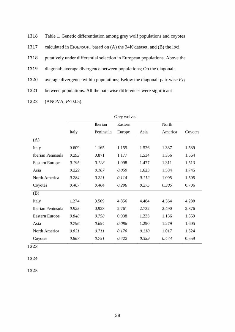
58

Table 1. Genetic differentiation among grey wolf populations and coyotes 1316

calculated in EIGENSOFT based on (A) the 34K dataset, and (B) the loci 1317

putatively under differential selection in European populations. Above the 1318

diagonal: average divergence between populations; On the diagonal: 1319

average divergence within populations; Below the diagonal: pair-wise FST 1320

between populations. All the pair-wise differences were significant 1321

(ANOVA, P<0.05). 1322

Grey wolves

Italy

Iberian

Peninsula

Eastern

Europe Asia

North

America Coyotes

(A)

Italy 0.609 1.165 1.155 1.526 1.337 1.539

Iberian Peninsula 0.293 0.871 1.177 1.534 1.356 1.564

Eastern Europe 0.195 0.128 1.098 1.477 1.311 1.513

Asia 0.229 0.167 0.059 1.623 1.584 1.745

North America 0.284 0.221 0.114 0.112 1.095 1.505

Coyotes 0.467 0.404 0.296 0.275 0.305 0.706

(B)

Italy 1.274 3.509 4.856 4.484 4.364 4.288

Iberian Peninsula 0.925 0.923 2.761 2.732 2.490 2.376

Eastern Europe 0.848 0.758 0.938 1.233 1.136 1.559

Asia 0.796 0.694 0.086 1.290 1.279 1.605

North America 0.821 0.711 0.170 0.110 1.017 1.524

Coyotes 0.867 0.751 0.422 0.359 0.444 0.559

1323

1324

1325

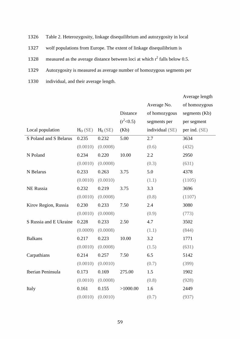
59

Table 2. Heterozygosity, linkage disequilibrium and autozygosity in local 1326

wolf populations from Europe. The extent of linkage disequilibrium is 1327

measured as the average distance between loci at which r2 falls below 0.5. 1328

Autozygosity is measured as average number of homozygous segments per 1329

individual, and their average length. 1330

Local population HO (SE) HE (SE)

Distance

(r2<0.5)

(Kb)

Average No.

of homozygous

segments per

individual (SE)

Average length

of homozygous

segments (Kb)

per segment

per ind. (SE)

S Poland and S Belarus

0.235

(0.0010)

0.232

(0.0008)

5.00

2.7

(0.6)

3634

(432)

N Poland

0.234

(0.0010)

0.220

(0.0008)

10.00

2.2

(0.3)

2950

(631)

N Belarus

0.233

(0.0010)

0.263

(0.0010)

3.75

5.0

(1.1)

4378

(1105)

NE Russia

0.232

(0.0010)

0.219

(0.0008)

3.75

3.3

(0.8)

3696

(1107)

Kirov Region, Russia

0.230

(0.0010)

0.233

(0.0008)

7.50

2.4

(0.9)

3080

(773)

S Russia and E Ukraine

0.228

(0.0009)

0.233

(0.0008)

2.50

4.7

(1.1)

3502

(844)

Balkans

0.217

(0.0010)

0.223

(0.0008)

10.00

3.2

(1.5)

1771

(631)

Carpathians

0.214

(0.0010)

0.257

(0.0010)

7.50

6.5

(0.7)

5142

(399)

Iberian Peninsula

0.173

(0.0010)

0.169

(0.0008)

275.00

1.5

(0.8)

1902

(928)

Italy

0.161

(0.0010)

0.155

(0.0010)

>1000.00

1.6

(0.7)

2449

(937)

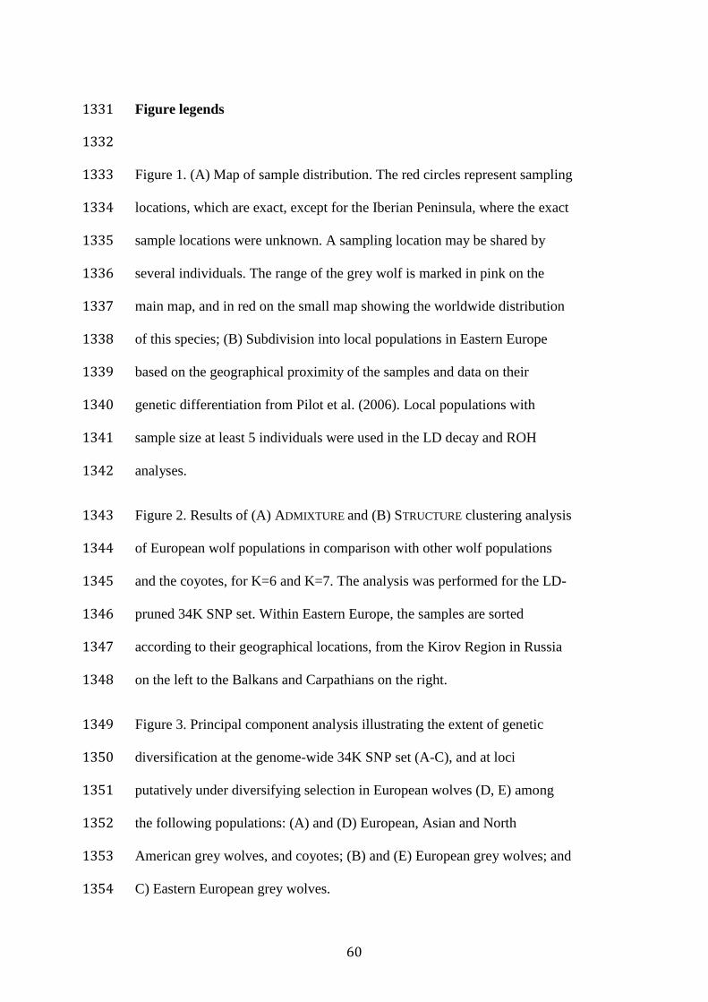
60

Figure legends 1331

1332

Figure 1. (A) Map of sample distribution. The red circles represent sampling 1333

locations, which are exact, except for the Iberian Peninsula, where the exact 1334

sample locations were unknown. A sampling location may be shared by 1335

several individuals. The range of the grey wolf is marked in pink on the 1336

main map, and in red on the small map showing the worldwide distribution 1337

of this species; (B) Subdivision into local populations in Eastern Europe 1338

based on the geographical proximity of the samples and data on their 1339

genetic differentiation from Pilot et al. (2006). Local populations with 1340

sample size at least 5 individuals were used in the LD decay and ROH 1341

analyses. 1342

Figure 2. Results of (A) ADMIXTURE and (B) STRUCTURE clustering analysis 1343

of European wolf populations in comparison with other wolf populations 1344

and the coyotes, for K=6 and K=7. The analysis was performed for the LD-1345

pruned 34K SNP set. Within Eastern Europe, the samples are sorted 1346

according to their geographical locations, from the Kirov Region in Russia 1347

on the left to the Balkans and Carpathians on the right. 1348

Figure 3. Principal component analysis illustrating the extent of genetic 1349

diversification at the genome-wide 34K SNP set (A-C), and at loci 1350

putatively under diversifying selection in European wolves (D, E) among 1351

the following populations: (A) and (D) European, Asian and North 1352

American grey wolves, and coyotes; (B) and (E) European grey wolves; and 1353

C) Eastern European grey wolves. 1354

61

1355

Figure 4. Evolutionary relationships among X chromosome haplotypes of 1356

females inferred using the neighbour-joining method. The distances were 1357

computed using the p-distance measure. Bootstrap support is shown if 1358

higher than 50% of 1000 replicates. 1359

Figure 5. (A) Extent of linkage disequilibrium in European wolf 1360

populations. Average genotypic association coefficient r2 is presented as a 1361

function of inter-SNP distance for each local wolf population. (B) 1362

Frequency distribution of runs of homozygosity in European wolf 1363

populations. (C) Temporal changes of NE in European wolves, with North 1364

American wolves presented for a comparison. 1365

Figure 6. Signatures of selection in the Iberian, Italian and Eastern European 1366

wolf populations inferred using the program BAYESCAN. The vertical axis 1367

indicates mean FST values between each of the three populations, and the 1368

horizontal axis indicates the logarithm of posterior odds (log(PO)). The 1369

vertical line indicates the log(PO) value corresponding to the false discovery 1370

rate threshold of 0.05. Loci on the right of this line are putatively under 1371

selection. 1372

1373

1374

1375

1376

62

Figure 1 1377

1378

1379

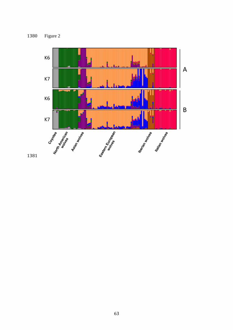
63

Figure 2 1380

1381

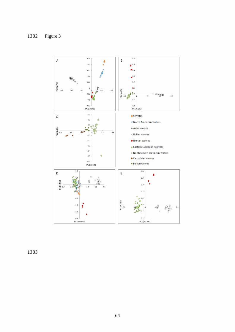
64

Figure 3 1382

1383

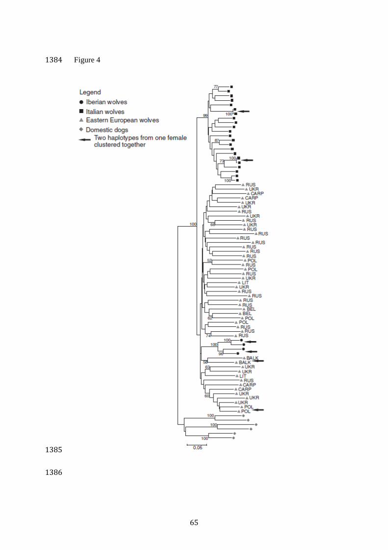
65

Figure 4 1384

1385

1386

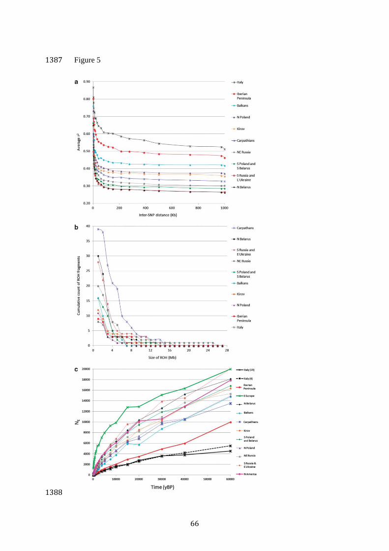
66

Figure 5 1387

1388

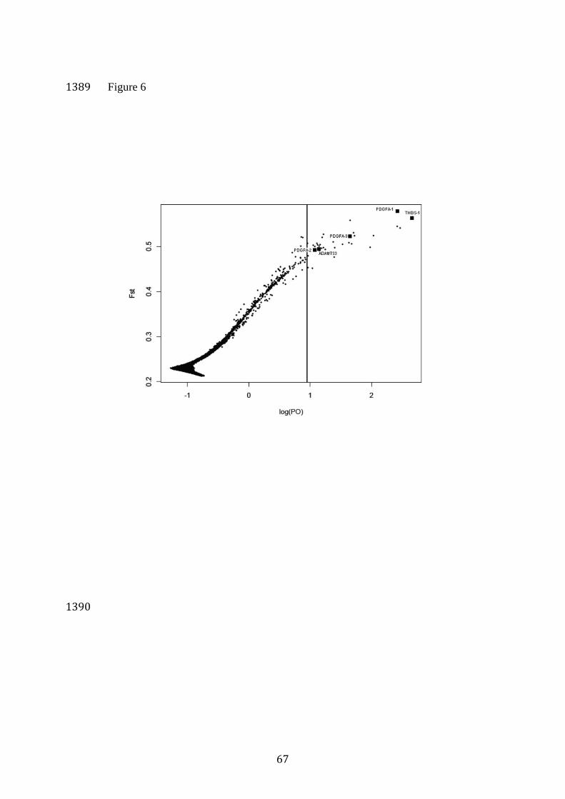
67

Figure 6 1389

1390