POLITECHNIKA WARSZAWSKA

WYDZIAŁ MATEMATYKI

I NAUK INFORMACYJNYCH

PRACA DYPLOMOWA INŻYNIERSKA

INFORMATYKA

Generowanie trójwymiarowych modeli roślin

Autor: Kamil Andrzej Ciosek

Promotor: Dr. Paweł Kotowski

Warszawa, Marzec 2008

Author’s signature / Podpis autora:

...................................................

Supervisor’s signature / Podpis promotora:

...................................................

WARSAW UNIVERSITY OF TECHNOLOGY

FACULTY OF MATHEMATICS

AND INFORMATION SCIENCE

B. Sc. THESIS

COMPUTER SCIENCE

Generating 3D Plants

Author: Kamil Andrzej Ciosek

Supervisor: Dr. Paweł Kotowski

Warsaw, March 2008

Abstract

The main focus of the present thesis is the analysis of modern methods of al-

gorithmic plant generation. First, a brief introduction is given to the necessary

formalisms: Lindenmayer systems and plane triangulations. It is followed by a de-

scription of each stage of the plant generation process. These include algorithms for

obtaining: leaf venation graph, leaf texture, stem texture, and the geometry and

topology of the whole plant. Finally account is given of the effort to implement

some of the described procedures in a program accompanying the thesis. In the pro-

gram, textures are obtained from transformed noise, a general plant description is

generated with a parametric Lindenmayer system and a purpose-built particle-based

algorithm is used to simulate leaf venation.

Streszczenie

Celem pracy jest analiza współczesnych metod algorytmicznego generowania

roślin oraz ich implementacja w dołączonym programie. Najpierw wprowadzone

są niezbędne formalizmy – systemy Lindenmayera i triangulacje na płaszczyźnie.

Następnie opisane są poszczególne części procesu generowania rośliny. W szczegól-

ności przedstawione są algorytmy generujące: graf żyłek na liściu, teksturę tła liścia,

teksturę łodygi oraz geometrię i strukturę całej rośliny. Na koniec opisane są kwestie

związane z implementacją zaprezentowanych algorytmów. Program dołączony do

pracy używa przekształconego szumu do generowania tekstur oraz parametrycznego

systemu Lindenmayera do generowania ogólnego schematu rośliny. Wzrost żyłek na

liściu jest natomiast symulowany z użyciem dedykowanego algorytmu opartego na

cząstkach.

2

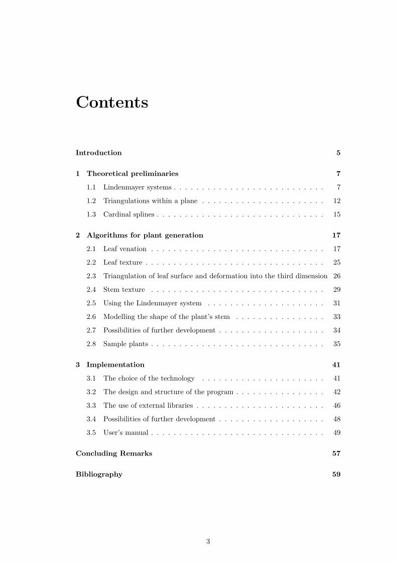
Contents

Introduction 5

1 Theoretical preliminaries 7

1.1 Lindenmayer systems . . . . . . . . . . . . . . . . . . . . . . . . . . . 7

1.2 Triangulations within a plane . . . . . . . . . . . . . . . . . . . . . . 12

1.3 Cardinal splines . . . . . . . . . . . . . . . . . . . . . . . . . . . . . . 15

2 Algorithms for plant generation 17

2.1 Leaf venation . . . . . . . . . . . . . . . . . . . . . . . . . . . . . . . 17

2.2 Leaf texture . . . . . . . . . . . . . . . . . . . . . . . . . . . . . . . . 25

2.3 Triangulation of leaf surface and deformation into the third dimension 26

2.4 Stem texture . . . . . . . . . . . . . . . . . . . . . . . . . . . . . . . 29

2.5 Using the Lindenmayer system . . . . . . . . . . . . . . . . . . . . . 31

2.6 Modelling the shape of the plant’s stem . . . . . . . . . . . . . . . . 33

2.7 Possibilities of further development . . . . . . . . . . . . . . . . . . . 34

2.8 Sample plants . . . . . . . . . . . . . . . . . . . . . . . . . . . . . . . 35

3 Implementation 41

3.1 The choice of the technology . . . . . . . . . . . . . . . . . . . . . . 41

3.2 The design and structure of the program . . . . . . . . . . . . . . . . 42

3.3 The use of external libraries . . . . . . . . . . . . . . . . . . . . . . . 46

3.4 Possibilities of further development . . . . . . . . . . . . . . . . . . . 48

3.5 User’s manual . . . . . . . . . . . . . . . . . . . . . . . . . . . . . . . 49

Concluding Remarks 57

Bibliography 59

3

4

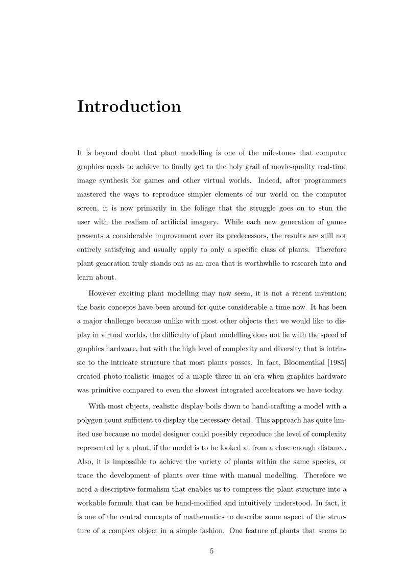
Introduction

It is beyond doubt that plant modelling is one of the milestones that computer

graphics needs to achieve to finally get to the holy grail of movie-quality real-time

image synthesis for games and other virtual worlds. Indeed, after programmers

mastered the ways to reproduce simpler elements of our world on the computer

screen, it is now primarily in the foliage that the struggle goes on to stun the

user with the realism of artificial imagery. While each new generation of games

presents a considerable improvement over its predecessors, the results are still not

entirely satisfying and usually apply to only a specific class of plants. Therefore

plant generation truly stands out as an area that is worthwhile to research into and

learn about.

However exciting plant modelling may now seem, it is not a recent invention:

the basic concepts have been around for quite considerable a time now. It has been

a major challenge because unlike with most other objects that we would like to dis-

play in virtual worlds, the difficulty of plant modelling does not lie with the speed of

graphics hardware, but with the high level of complexity and diversity that is intrin-

sic to the intricate structure that most plants posses. In fact, Bloomenthal [1985]

created photo-realistic images of a maple three in an era when graphics hardware

was primitive compared to even the slowest integrated accelerators we have today.

With most objects, realistic display boils down to hand-crafting a model with a

polygon count sufficient to display the necessary detail. This approach has quite lim-

ited use because no model designer could possibly reproduce the level of complexity

represented by a plant, if the model is to be looked at from a close enough distance.

Also, it is impossible to achieve the variety of plants within the same species, or

trace the development of plants over time with manual modelling. Therefore we

need a descriptive formalism that enables us to compress the plant structure into a

workable formula that can be hand-modified and intuitively understood. In fact, it

is one of the central concepts of mathematics to describe some aspect of the struc-

ture of a complex object in a simple fashion. One feature of plants that seems to

5

be helpful in doing so is the fact that they display a certain degree of self-similarity.

Of course, this fractal-like behaviour does not encompass every aspect of the plant

at every scale, but still, it is quite helpful. In this respect, this thesis describes the

concept of Lindenmayer systems: a type of formal grammars that is especially well-

suited for the modelling of plants and that allows the user to easily exploit whatever

self-similarity the plant has.

One issue that often arises during the use of plant-generating algorithms is the

question of how good they are at modelling the biological processes that happen

inside the plant. While this certainly helps because it usually means the parameters

of the model may be easily tweaked to modify the results and the developmental

of the plant structures traced in time, it is not a precondition for a good model.

Computer science is inherently a phenomenological science, so it is really the program

output that ultimately matters. It has therefore been decided that the way in

which a given algorithm imitates what happens inside the plant is only of secondary

importance.

The following chapters give an account of experiments with Lindenmayer sys-

tems, as well as of efforts to patch them up by adding external algorithms to model

the aspects of the plant that they poorly represent (most notably, leaf venation

patterns). It also describes a program that implements some of the presented ideas.

6

Chapter 1

Theoretical preliminaries

This chapter gives a brief and practically-oriented discussion of the theoretical con-

cepts that one needs to master to be able to implement plant generation algorithms.

1.1 Lindenmayer systems

The following sections introduce the concept of Lindenmayer systems, a variation

of formal grammars widely applied to plant generation. They were first introduced

by Aristid Lindenmayer as a means of modelling the growth of algae, but were

later given a more thorough theoretical description and applied to many different

problems. The theoretical part of this section is based on Salomaa [1973].

Deterministic context-free Lindenmayer systems are described in a relatively

thorough way, while their modifications, which increase generative power, are only

described briefly.

Definition. A deterministic context free Lindenmayer system (D0L-system) is a

tuple < V, ω, P >.

1. V - is a set of symbols.

2. ω ∈ V - is the axiom or start symbol.

3. P ⊂ V × V ∗ : (∀a)(∃!p)((a, p) ∈ P ) is the set of productions.

Note that the right side of the production may be empty (erasable productions

are permissible) and that Lindenmayer systems do not differentiate between terminal

or non-terminal symbols. Also note that each symbol is the left side of exactly one

production (hence the determinism).

The defining feature of Lindenmayer systems will now be presented: the basic

relation that is used to generate words.

7

Definition. The arrow relation → ⊂ V + × V ∗ is defined as follows: P → Q iff P

can be expressed as a sequence of symbols P = p1, p2, ..., pn : pi ∈ V and Q can be

expressed as a sequence of (possibly empty) strings Q = q1, q2, ..., qn ∈ V ∗ such that

n > 0 and for each i there exists a production from pi to qi, i.e. (∀i)(pi, qi) ∈ P .

Note that the difference between ordinary grammars and Lindenmayer systems

lies in the fact that we substitute all symbols at once. Also note that, given a string

from V ∗, the concatenation of the transformations of each constituent letter of the

string is defined unambiguously and is trivial to compute. This is in strict opposition

to context-free grammars, where special care needs to be taken to avoid ambiguity.

In practical applications, we start off with the axiom and iterate the→ relation a

fixed number of steps. The number of steps is considered a parameter. Normally, this

parameter represents the ”depth” of simulation, for example the level of development

of the plant being modelled. Below, a simple example of a deterministic context-free

Lindenmayer system is presented. A more elaborate example, which can be used to

model plants will be given later.

V = {A,B,C}

ω = A

The set P is contains the following productions:

A→ BC

B → AC

Note that we have omitted the production from C. This is common practice, and

means that C → C. After three iterations, this system yields:

ω = A→ BC → ACC → BCCC

Definition. The relation ⇒ ⊂ V + × V ∗ is the reflexive transitive closure of →.

In short, P ⇒ Q for all Q which are obtainable (in the sense of → ) from P . We

will use this relation to define the language generated by a Lindenmayer system as

all strings obtainable form the axiom with an arbitrary number of iterations.

Definition. A language generated by a Lindenmayer system < V, ω, P > is defined

as {S : ω ⇒ S}. A language generated by a D0L system is called a D0L language.

Observation. For each string s in a D0L language, there exists an integer k, such

that the string s is obtained from the axiom ω of a D0L system generating this

language in exactly k steps (i.e. using the → relation exactly k times).

8

The preceding statement is obvious but needs to be mentioned explicitly be-

cause we will be using continuously in the reminder of this section. It will now

be attempted to relate this newly introduced concept co ”classical” levels of the

Chomsky hierarchy. Note, however, that although these properties are instructive,

they are only of secondary importance for the modelling of plants as we usually only

iterate the system a specific number of times and are not really interested in the

”limit” properties of the system.

Observation. There exist regular D0L languages.

Proof. Consider the language {A}, generated by the system ω → A.

Observation. There exist context-free D0L languages that are not regular.

Proof. Consider the language {s : s = A2nB2n , n ≥ 1}, generated by the system

ω → AB,A→ AA,B → BB.

Observation. There exist context-sensitive D0L languages that are not context free.

Proof. Consider the language {s : s = A2nB2nC2n , n ≥ 1}, generated by the system

ω → ABC,A→ AA,B → BB,C → CC.

Observation. There exist regular languages that are not D0L.

Proof. Consider the language {A,AA}. Assume it is generated by a D0L system.

Therefore, either A⇒ AA or AA⇒ A. The latter is impossible, because this would

mean that A ⇒ ε, and therefore the empty word ε would belong to the language.

Therefore A ⇒ AA. However, this means that the word AAAA belongs to the

language generated by the D0L system, which is a contradiction.

Observation. There exist context-free languages that are neither D0L nor regular.

Proof. Consider the language {A,AA} ∪ {s : s = A2nB2n , n ≥ 1}. Assume it is

generated by a D0L system, proceed as in the previous example.

Observation. There exist context-sensitive languages that are neither D0L nor

context-free.

Proof. Consider the language {A,AA} ∪ {s : s = A2nB2nC2n , n ≥ 1}. Assume it is

generated by a D0L system, proceed as in the previous example.

Theorem. All D0L languages are context sensitive.

9

Proof. We shall construct a context-sensitive grammar G that simulates deriva-

tion in an arbitrary D0L system < V, ω, P >. Consider the grammar G =<

{A,B,C,D}, V, A, PG >, where the set PG contains the productions listed below.(1) A→ BωB

(2*) Bv → BCv (one production for each v ∈ V )

(3*) Cv → RC (one grammar production for each D0L production (v,R))

(4) CB → DB

(5*) vD → Dv (one production for each v ∈ V )

(6) BD → B

(7) B → ε

It is easy to see how this grammar works: production (1) sets the initial state of

the simulation. The symbols B function as boundary markers. Using a production

of the form (2*) results in the creation of the symbol C, which traverses the word

and replaces the left side of each D0L-production with its right side using produc-

tions (3*). Once the end of the string is reached, production (4) creates a special

”return” symbol D that returns to the beginning of the word using productions

(5*). Production (6) is used to eliminate the symbol D. This corresponds to the

end of an iteration of the D0L-system. There are now two options, either to use the

production (7) and terminate the derivation or to use a production (2*) and start

one more iteration step.

Therefore, every D0L-language is generated by a context-sensitive grammar.

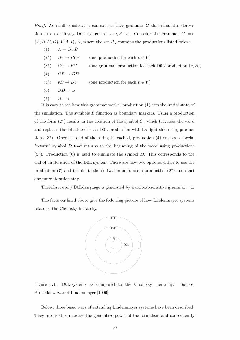
The facts outlined above give the following picture of how Lindenmayer systems

relate to the Chomsky hierarchy.

Figure 1.1: D0L-systems as compared to the Chomsky hierarchy. Source:

Prusinkiewicz and Lindenmayer [1996].

Below, three basic ways of extending Lindenmayer systems have been described.

They are used to increase the generative power of the formalism and consequently

10

to be able to model more intricate structures.

The first modification is quite obvious: we can add non-determinism by dropping

the requirement (∀a)(∃!p)((a, p) ∈ P ) on the set of productions and replacing it with

(∀a)(∃p)((a, p) ∈ P ). The motivation for this in practical approaches is that we want

to add variation to the generated model (for example to reflect the fact that plants

of the same species look alike but are not strictly identical). In fact, we usually

first create a deterministic system and then extend it by adding non-determinism

to certain productions. To facilitate this approach, a probability function may be

added which maps each production to a probability value (of course, probabilities

of productions with the same left side sum to 1).

Another way of increasing the generative power of Lindenmayer systems is to

add context-sensitivity. Systems where each production has both a left context and

a right context are called 2L-systems (the contexts contain only one symbol each).

The set of productions of context-sensitive systems is formally defined below.P ⊂ (V × V × V )× V ∗ (for 2L-systems)

P ⊂ (V × V )× V ∗ (for 1L-systems)Systems where either all productions have a left context or all productions have

a right context are called 1L systems. These classes are distinct (i.e. there exist

languages that are generated by 2L-systems but not 1L-systems). Likewise, there

exist languages generated by 1L-systems but not context-free systems. The practical

motivation of using context-sensitivity is the transmission of signals (for example,

from one part of the plant to another).

Yet another approach is through adding a real numerical value (or many such

values) to each symbol and then using parametric expressions and conditions. The

set Σ of formal parameters in introduced and the axiom is redefined as ω ∈ (V ×

R∗)+. The discussion of parametric Lindenmayer systems presented here is based on

Hanan [1992]. From the drawing perspective, parametric systems have the following

motivation: they allow plotting lines of non-rational length (like the diagonal of a

unit square) and allow for easy shrinking of plant segments that appear later in the

derivation process (through using a parameter that corresponds to segment length).

Productions of parametric Lindenmayer systems are of the form given below.

P ⊂ (V × Σ∗)× C(Σ)× (V × E(Σ)∗)∗

In the above formula, C(Σ) corresponds to the set of possible well-formed boolean

conditions operating on formal parameters from the set Σ, wile E corresponds to

the set of possible well-formed arithmetic expressions with formal parameters from

the set Σ. Note that each symbol may have any number of parameters, or not

11

parameters at all. The influence of these addenda on the process of derivation is

that: (i) values of parameters are evaluated for each iteration step, (ii) a production

may only be used if its condition evaluates to true. Conditions is productions with

the same left side have to be mutually exclusive, unless we also want to add non-

determinism. A sample parametric system that can be used to generate a plant will

be given in the next chapter.

Of course, these three approaches may be combined. In the program accompa-

nying this thesis, only the last of the mentioned modifications was used, i.e. deter-

ministic context-free parametric Lindenmayer systems have been implemented.

1.2 Triangulations within a plane

The discussion of Delaunay triangulations presented here is based on Goodman and

O’Rourke [1997]. They describe triangulations of arbitrary dimensionality, but the

plant generation algorithms described in this thesis only require two-dimensional

triangulations. Therefore, only two-dimensional triangulations will be described

here. Also, the algorithms used to compute the triangulations are not given (the

program used an external library, CGAL, to accomplish this task). In the program,

triangulations are used as part of two algorithms used by the program: the vein

growth algorithm, which uses Urquhart triangulation as an approximation of the

relative neighbourhood graph as well as the leaf deformation algorithm, which uses

a constrained Delaunay triangulation to create leaf mesh.

Definition. Given a set S of points within R2, three points A,B,C ∈ S are said

to form a Delaunay triangle iff the circumscribed circle of this triangle (A,B,C)

contains no point from S − {A,B,C}.

Definition. Given a set S of points within R2, a Delaunay triangulation DT (S) is

the set of all Delaunay triangles built of points from S.

Definition. Given a set S of points within R2, and a set of edges E connecting

some of the points from S, two points p, q are said to be visible from each other if

the line from p to q does not intersect any edge from E.

Definition. Given a set S of points within R2, and a set of constraint edges E with

endpoints from S a constrained Delaunay triangulation CDT (S,E) is the set of all

triangles built of points from S such that the circumscribed circle of each triangle

contains no point from S − {A,B,C} visible from the interior of the triangle with

respect to E.

12

Observation. A constrained Delaunay triangulation is not necessarily a Delaunay

triangulation.

Figure 1.2: Delaunay and constrained Delaunay triangulations of the same point set.

The constraint edge is dashed. Delaunay triangulation reproduced from Andrade

and de Figueiredo [2003].

Definition. Given a Delaunay triangulation DT (S), an Urquhart triangulation

UT (S) is a graph obtained by removing the longest edge from each triangle of DT (S).

Observation. UT (S) ⊂ DT (S).

Definition. Given a set S of points within R2, two points p, q ∈ S are relative

neighbours with respect to S iff

∀r ∈ S d(p, q) ≤ max(d(p, r), d(q, r))

where d(a, b) denotes Euclidean distance between points a, b.

A geometric interpretation of relative neighbourhood is given in the following

figure.

Figure 1.3: Points P,Q are relative neighbours iff there are no points in the grey

area (called a lune). Source: Andrade and de Figueiredo [2003].

Definition. Given a set S of points within R2, the graph RNG(S) is a graph such

that its vertices are points from S. Two points are connected in the graph if they are

relative neighbours with respect to S.

While introducing the relative neighbourhood graph, Toussaint [1980] showed

the following:

13

Theorem. RNG(S) ⊆ DT (S)

Observation. RNG(S) ⊆ UT (S). For some sets S, RNG(S) ⊂ UT (S).

Proof. First, we will show that RNG(S) ⊆ UT (S).

Indeed, consider a triangle (A,B,C) ⊂ DT (S). It suffices to show that the

longest edge of this triangle cannot belong to RNG(S). Assume the longest edge is

(A,B). Observe that point C belongs to the lune (corresponds to the grey are in

the figure) defined by points (A,B). Therefore (A,B) 6∈ RNG(S).

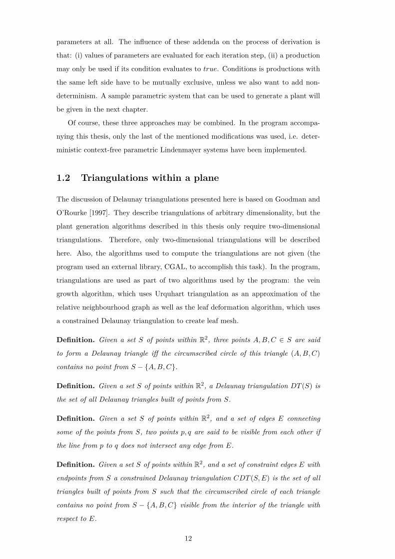
We still have to show that RNG(S) 6= UT (S). This is demonstrated in the

following figure (the edge E belongs to UT (S) but not to RNG(S).

Figure 1.4: Urquhart and relative neighbourhood graphs of the same point set.

Source: Andrade and de Figueiredo [2003].

In view of the previous observation, it seems interesting to know how many edges

of the Urquhart triangulation make it into the relative neighbourhood graph. It

turns out that a great majority does. In fact, Urquhart first proposed the Urquhart

graph as a way of fast evaluation of the relative neighbourhood graph. Empirical

tests on random graphs by Andrade and de Figueiredo [2003] show that on average,

the relative neighbourhood graph has only about 2% less edges than the Urquhart

graph.

Therefore, the Urquhart graph is a good way of approximating the relative neigh-

bourhood in application where accuracy is not critical. This is the approach taken

during the development of the program accompanying this thesis. This has the ad-

vantage that very fast library routines for computing Delaunay triangulations are

readily available and it is trivial to obtain the Urquhart graph from the Delaunay

graph. There exist algorithms for obtaining RNG(S) from DT (S) in time O(nlogn),

but these are very complicated. Also, Runions et al. [2005] have investigated the

effects of using this approximation while simulating leaf venation and found them

to be negligible.

14

1.3 Cardinal splines

This brief description is based on Salomon [1999]. It by no means exhaustive and

only describes the aspects of cardinal spline that have been important to the writing

of the program.

Definition. A cubic spline is a set of polynomials of degree 3 that pass through a set

of data points in such a way that they connect in a continuous way (i.e. the curves

meet and their tangents match).

Given a set of points, each polynomial in the spline built upon these points

should pass through two points and have certain tangent values at those points.

The following observation states that this defines the polynomial uniquely.

Observation. Given two points P0,P1 and two tangent vectors T0,T1, a polyno-

mial of the form f(t) = At3 + Bt2 + Ct + D f : [0, 1] → R × R is uniquely defined

by the conditions: f(0) = P0, f(1) = P1,dfdt (0) = T0,

dfdt (1) = T1.

Proof. This follows directly from substituting f for At3 + Bt2 + Ct + D in the

four conditions and solving the resulting equations for A,B,C,D, obtaining A =

2P0 − 2P1 + T0 + T1,B = 3(P1 −P0)− 2T0 −T1,C = T0,D = P0.

The question remains, however, how to pick the tangent values T0,T1. One way

of doing this is to require that the whole spline be second-order continuous (that

the second derivatives match at the connecting points). In this case the curve is

uniquely defined by the point locations and tangents at the endpoints. An obvious

advantage is that the curve is smoother. However, the resulting spline may change

along the whole length if just one point is moved, or the endpoint tangent is changed.

If the spline is to be used as an element of user interface, this is counter-intuitive for

the average user. Therefore, it seems adequate to sacrifice second-order continuity

for the “locality” property of the curve, i.e. for the fact that, if the user moves a

point within the curve, only a fixed number of curve segments closest to this point

change their shape. One way of doing this is through cardinal splines. With cardinal

splines, the tangents are defined in the following way.

Ti = (1− c)(Pi+1 −Pi−1)/2

In this formula, P−1 stands for the point that precedes point P0 within the curve,

and P2 is the point behind P1. Please not that endpoint tangents need to be either

specified explicitly or assumed to point into the direction of the next point (for the

start on the curve) and previous point (for the end of the curve). The parameter

15

c is corresponds to the curve tension. If c = 0, the spline is called a Catmull-Rom

spline. This is the default value used by Microsoft GDI+.

It is often necessary to calculate the length of the spline curve. In the leaf gen-

eration program, this is required by the algorithm that deforms the leaf along a

predefined curve. It follows from elementary calculus that for an arbitrary continu-

ous curve specified by a parametric equation f : [0, 1] → R × R, the length of this

curve is given by the following formula:

l =∫ 1

0g(t)dt, g(t) =

√√√√(dfdt

)2

x+(df

dt

)2

y

For cardinal splines, this integral has to be evaluated numerically. To do this, Gauss-

Legendre quadrature has been used. Using it, the curve length can be approximated

using the formula below (source: Wikipedia).

l ≈ 12

N∑i=1

wig

(12xi +

12

)

In this formula, xi and wi denote the quadrature abscissas and weights respectively.

For a given N , these are fixed constants. In the program accompanying the thesis,

it turned out that it sufficed to use N = 5 to achieve good results.

16

Chapter 2

Algorithms for plant generation

This chapter addresses the core issues related to plant generation. While the whole

process revolves around Lindenmayer systems, auxiliary mechanisms need to be

added to make the plants appear realistic. In the following subsections, a discussion

is given of the modules used for the generation of various aspects of plants.

2.1 Leaf venation

Modelling leaf venation is quite imperative to achieving the proper looks of a mod-

elled plant. This is due to the fact that the surface of plant leaves is usually bigger

and more prominent to the viewer than other features of the plant. Therefore due

care must be exercised to ensure that an adequate algorithm is employed. The most

widely used approaches to the modelling of venation patterns are discussed below.

Taulor-Hell and Baranoski [2002] provide a thorough list of methods used to

date, ranging from simple texture mapping of scanned leaves to modern procedu-

ral approaches. In particular, they evaluate the following methods (the list below

summarizes the authors’ findings):

1. Lindenmayer systems, which have the advantage of almost unlimited flexibility,

but need to be extended with a geometric formalism to provide realistic models

of plant organs,

2. implicit surfaces, applied to leaf venation by Bloomenthal [1995], who devel-

oped very intricate apparatus for modelling, modifying and blending surfaces

with the help of skeletons, which, however, does not solve the issue of getting

a flat leaf venation pattern in the first place (he used a scanned leaf),

3. particle systems, which are computationally expensive and complicated but

flexible,

17

4. cellular texture basis functions, on which it is impossible for me to comment

because literature on the subject is unavailable.

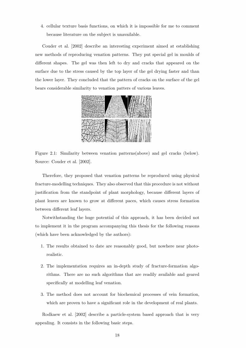
Couder et al. [2002] describe an interesting experiment aimed at establishing

new methods of reproducing venation patterns. They put special gel in moulds of

different shapes. The gel was then left to dry and cracks that appeared on the

surface due to the stress caused by the top layer of the gel drying faster and than

the lower layer. They concluded that the pattern of cracks on the surface of the gel

bears considerable similarity to venation patters of various leaves.

Figure 2.1: Similarity between venation patterns(above) and gel cracks (below).

Source: Couder et al. [2002].

Therefore, they proposed that venation patterns be reproduced using physical

fracture-modelling techniques. They also observed that this procedure is not without

justification from the standpoint of plant morphology, because different layers of

plant leaves are known to grow at different paces, which causes stress formation

between different leaf layers.

Notwithstanding the huge potential of this approach, it has been decided not

to implement it in the program accompanying this thesis for the following reasons

(which have been acknowledged by the authors):

1. The results obtained to date are reasonably good, but nowhere near photo-

realistic.

2. The implementation requires an in-depth study of fracture-formation algo-

rithms. There are no such algorithms that are readily available and geared

specifically at modelling leaf venation.

3. The method does not account for biochemical processes of vein formation,

which are proven to have a significant role in the development of real plants.

Rodkaew et al. [2002] describe a particle-system based approach that is very

appealing. It consists in the following basic steps.

18

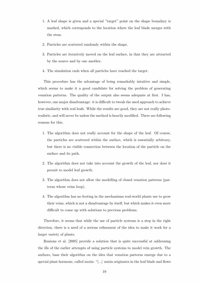
1. A leaf shape is given and a special ”target” point on the shape boundary is

marked, which corresponds to the location where the leaf blade merges with

the stem.

2. Particles are scattered randomly within the shape.

3. Particles are iteratively moved on the leaf surface, in that they are attracted

by the source and by one another.

4. The simulation ends when all particles have reached the target.

This procedure has the advantage of being remarkably intuitive and simple,

which seems to make it a good candidate for solving the problem of generating

venation patterns. The quality of the output also seems adequate at first. I has,

however, one major disadvantage: it is difficult to tweak the used approach to achieve

true similarity with real leafs. While the results are good, they are not really photo-

realistic, and will never be unless the method is heavily modified. There are following

reasons for this.

1. The algorithm does not really account for the shape of the leaf. Of course,

the particles are scattered within the surface, which is essentially arbitrary,

but there is no visible connection between the location of the particle on the

surface and its path.

2. The algorithm does not take into account the growth of the leaf, nor does it

permit to model leaf growth.

3. The algorithm does not allow the modelling of closed venation patterns (pat-

terns whose veins loop).

4. The algorithm has no footing in the mechanisms real-world plants use to grow

their veins, which is not a disadvantage by itself, but which makes it even more

difficult to come up with solutions to previous problems.

Therefore, it seems that while the use of particle systems is a step in the right

direction, there is a need of a serious refinement of the idea to make it work for a

larger variety of plants.

Runions et al. [2005] provide a solution that is quite successful at addressing

the ills of the earlier attempts of using particle systems to model vein growth. The

authors, base their algorithm on the idea that venation patterns emerge due to a

special plant hormone, called auxin: “[...] auxin originates in the leaf blade and flows

19

toward existing veins, which transport it to the leaf base. During this flow, auxin is

canalized into narrow paths [...]. These paths gradually differentiate into new vein

segments. Experimental evidence suggests that auxin sources may be discrete.”

To account for this hormone, the algorithm uses two kinds of particles: source

particles, representing auxin and node particles, representing vein segments. The

algorithm is an iterative process that tries to reproduce the way in which the sources

and nodes relate to one another on the leaf surface.

It has been decided that the last algorithm is the most appropriate candidate for

implementation in the program accompanying this thesis. It is described in detail

in the following sections. First, a simplified version will be discussed that can only

model open (non-looping) venation patterns. Then it will be extended to account

for closed (looping) patterns. Please note that, unless otherwise noted, all the ideas

discussed in this context are taken from Runions et al. [2005].

The following list presents the inputs to the algorithm. For convenience it has

been assumed that x, y coordinates on the leaf surface are normalized to the [0, 1]

interval.

1. An initial shape of the leaf. It may be defined in an arbitrary way provided it

does not comprise disjoint regions.

2. A special point on the initial leaf shape, the leaf origin. It is considered to be

the first leaf node.

3. A growth function f(x, y, t) : [0, 1]× [0, 1]×N→ [0, 1]× [0, 1]. It tells us where

a particle, which is at location (x, y) at the moment t, will be at the moment

t+ 1.

4. A procedure of adding new sources at simulation step t. It will be explained

later on and does not really need to be formalised.

5. A value g, which corresponds to the distance by which a vein grows in one

iteration step.

6. A value d, which corresponds to the distance between a node and a source at

which we assume that the node has reached the source.

7. A value dSS , which corresponds to the minimum distance between a newly-

added source and existing sources.

8. A value dSN , which corresponds to the minimum distance between a newly-

added source and existing nodes.

20

9. A value s, which corresponds to the number of sources that are added at each

iteration of the algorithm.

10. A value i, which specifies the number of iterations of the algorithm.

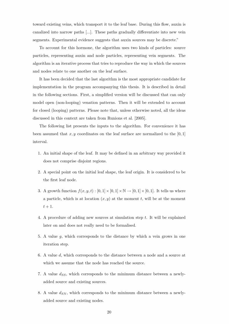
The procedure is summarised in the following basic steps.

1. At a given point of time, the leaf has a certain shape and a certain number

of hormone sources is scattered within the shape. Each source has a specific

location. Also, node particles added during previous iteration steps appear on

the surface.

2. For each source, exactly one vein node is chosen, which is said to influence the

source. It is the node nearest to the source, or if there are many nodes at the

same distance, any one of them is picked at random. Note that one node may

by influenced by many sources or no sources at all.

3. For each vein node, which is influenced by at least one source, its growth di-

rection is calculated, which is the arithmetic average of the directions pointing

towards the sources that influence the node. The node then grows in the cal-

culated direction by distance g i.e. a new vein node is created and a logical

edge is created between the new node and the old node, which will later be

rendered as a vein segments. The old node remains on the leaf and may still

grow in further stages of the process.

4. Sources that have been reached by a node are deleted. A vein node is consid-

ered to have reached the source if it is within a certain distance d from the

source.

5. The leaf grows. This means that all particles on the leaf may change location

according to the pre-defined function f and that new sources may be added

to the leaf, in a way that reflects the kind growth of the surface we wish to

model. The leaf boundary also grows.

The algorithm returns the venation graph (in this case, a tree).

The described procedure needs some clarification as to the various ways in which

the leaf may grow. The authors of the algorithm list three most common possibilities:

1. Marginal growth: only the leaf boundary grows. The growth is homothetic

with respect to the leaf origin. Particles do not change their location between

steps.

21

2. Uniform growth: both the boundary and existing particles grow. The growth

is likewise homothetic with respect to the leaf origin.

3. Non-uniform anisotropic growth. This is the general case in which the leaf

surface changes its shape as defined by an arbitrary function.

This distinction is important because the authors report vastly different results

depending on the kind of growth function used and the speed of growth. However,

good results can usually be achieved without resulting to the most general case,

which is relatively difficult to implement.

It is also important to clarify the way in which new auxin sources are added to

the leaf surface. The authors describe two ways.

1. At each iteration step, a given number of sources s is placed on the leaf surface.

Thy are scattered all over the leaf.

2. At each iteration step, sources are added only to the area by which the leaf

shape has grown. This is best done by abandoning the use of the s parameter

and pre-computing the source distribution before the simulation begins.

In either case, the sources are added using a dart-throwing algorithm in such

a way that the distance between a new source and an existing source is not closer

than dSS and the distance between a new source and an existing node is not closer

than dSN (i.e. the program picks random locations until it satisfies algorithm re-

quirements).

Once the iterative process has completed, we have a graph representing the

generated venation pattern. What we would like to have, however, is the texture of

the actual veins. To get it, we need to account for one vastly important aspect of

leaf venation: the width of the veins. First, we observe that the venation pattern of

leaf generated using the described algorithm has the topology of a tree. This means

that the edges (vein segments) may be sorted with respect to their distance from

the tree root (leaf origin). Therefore, it is possible to mark the edges which are

the furthest from the root (the thinnest veins) as having width 1 . The with of the

remaining edges can then be assumed to follow from the formula rnparent =∑rnchildi

We calculate the widths of edges that are farther from the root first and then use

these values to calculate the nearer ones. The process is repeated till we reach the

root node. The authors of the algorithm note that while the formula has biological

footing for n = 3, it may also be treated as yet another user-specified parameter.

It may be deduced that the algorithm has the following shortcomings:

22

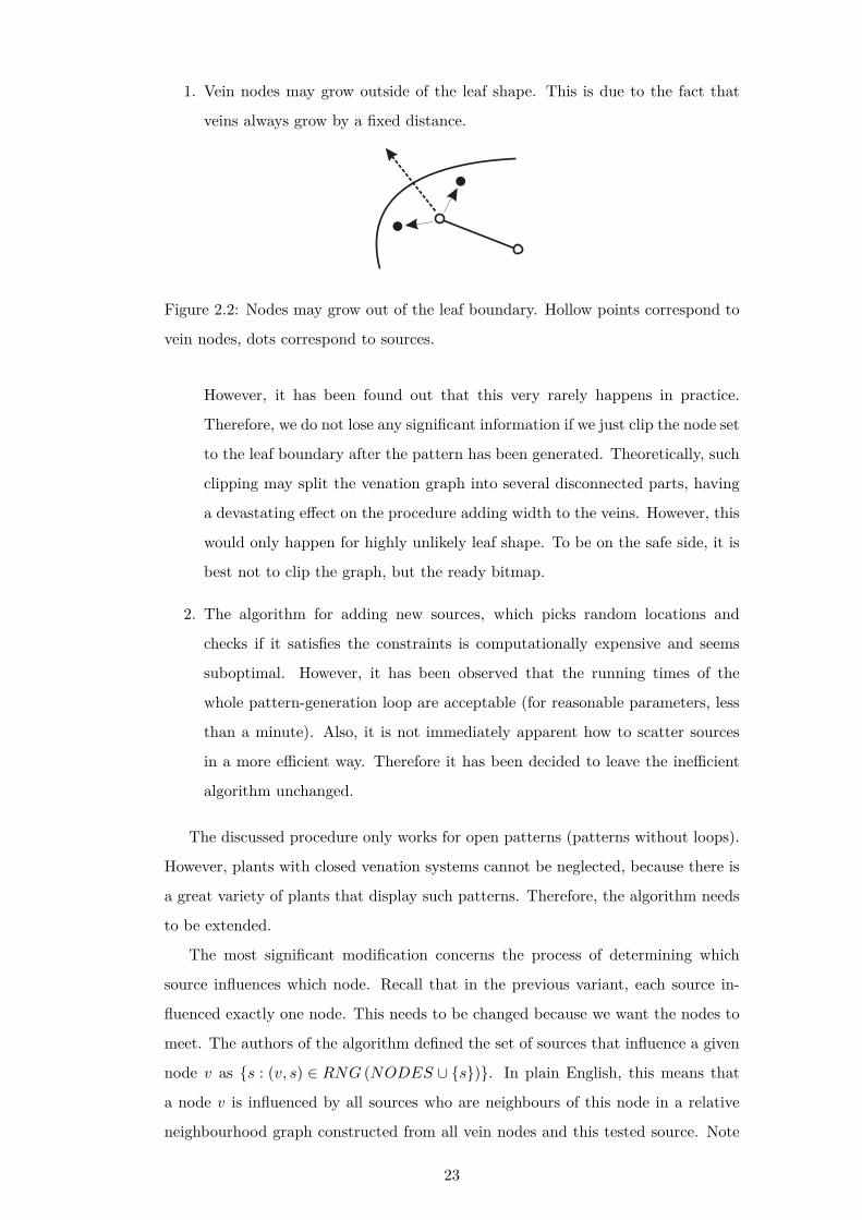
1. Vein nodes may grow outside of the leaf shape. This is due to the fact that

veins always grow by a fixed distance.

Figure 2.2: Nodes may grow out of the leaf boundary. Hollow points correspond to

vein nodes, dots correspond to sources.

However, it has been found out that this very rarely happens in practice.

Therefore, we do not lose any significant information if we just clip the node set

to the leaf boundary after the pattern has been generated. Theoretically, such

clipping may split the venation graph into several disconnected parts, having

a devastating effect on the procedure adding width to the veins. However, this

would only happen for highly unlikely leaf shape. To be on the safe side, it is

best not to clip the graph, but the ready bitmap.

2. The algorithm for adding new sources, which picks random locations and

checks if it satisfies the constraints is computationally expensive and seems

suboptimal. However, it has been observed that the running times of the

whole pattern-generation loop are acceptable (for reasonable parameters, less

than a minute). Also, it is not immediately apparent how to scatter sources

in a more efficient way. Therefore it has been decided to leave the inefficient

algorithm unchanged.

The discussed procedure only works for open patterns (patterns without loops).

However, plants with closed venation systems cannot be neglected, because there is

a great variety of plants that display such patterns. Therefore, the algorithm needs

to be extended.

The most significant modification concerns the process of determining which

source influences which node. Recall that in the previous variant, each source in-

fluenced exactly one node. This needs to be changed because we want the nodes to

meet. The authors of the algorithm defined the set of sources that influence a given

node v as {s : (v, s) ∈ RNG (NODES ∪ {s})}. In plain English, this means that

a node v is influenced by all sources who are neighbours of this node in a relative

neighbourhood graph constructed from all vein nodes and this tested source. Note

23

that we need a different graph for checking each source. In the program, UT is

used instead of RNG as described in the previous chapter. Once we identify the

influencing sources, we calculate the direction like we did previously.

The second modification concerns the deletion of sources from the graph. Pre-

viously, we just deleted the source as soon as a node came close enough. This has

to be changed, because when a closed pattern forms, one vein may reach the source

well ahead of the other. Therefore, once the first node reaches the source, the source

is not deleted, but merely tagged as being a candidate for deletion. The nodes ap-

proaching it (i.e. those which are influenced by the source) are also tagged. The

tags are inherited by the node that grows from the tagged node in the next itera-

tion step (of course, the parent node loses its tag). The source is only deleted if all

approaching nodes have either reached the source or moved a certain distance away

from it (this “forgetting” distance is an additional program parameter).

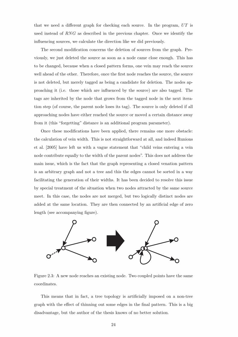
Once these modifications have been applied, there remains one more obstacle:

the calculation of vein width. This is not straightforward at all, and indeed Runions

et al. [2005] have left us with a vague statement that “child veins entering a vein

node contribute equally to the width of the parent nodes”. This does not address the

main issue, which is the fact that the graph representing a closed venation pattern

is an arbitrary graph and not a tree and this the edges cannot be sorted in a way

facilitating the generation of their widths. It has been decided to resolve this issue

by special treatment of the situation when two nodes attracted by the same source

meet. In this case, the nodes are not merged, but two logically distinct nodes are

added at the same location. They are then connected by an artificial edge of zero

length (see accompanying figure).

Figure 2.3: A new node reaches an existing node. Two coupled points have the same

coordinates.

This means that in fact, a tree topology is artificially imposed on a non-tree

graph with the effect of thinning out some edges in the final pattern. This is a big

disadvantage, but the author of the thesis knows of no better solution.

24

All aspects of the algorithm have been implemented in the accompanying pro-

gram, barring the simulation of leaf growth. Leaf growth is an important aspect of

the model, but it had to be omitted because of the limited time available to prepare

the program. Also, it was not the purpose of this thesis to model the process of

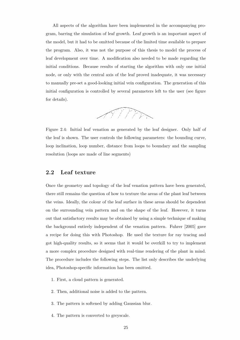
leaf development over time. A modification also needed to be made regarding the

initial conditions. Because results of starting the algorithm with only one initial

node, or only with the central axis of the leaf proved inadequate, it was necessary

to manually pre-set a good-looking initial vein configuration. The generation of this

initial configuration is controlled by several parameters left to the user (see figure

for details).

Figure 2.4: Initial leaf venation as generated by the leaf designer. Only half of

the leaf is shown. The user controls the following parameters: the bounding curve,

loop inclination, loop number, distance from loops to boundary and the sampling

resolution (loops are made of line segments)

2.2 Leaf texture

Once the geometry and topology of the leaf venation pattern have been generated,

there still remains the question of how to texture the areas of the plant leaf between

the veins. Ideally, the colour of the leaf surface in these areas should be dependent

on the surrounding vein pattern and on the shape of the leaf. However, it turns

out that satisfactory results may be obtained by using a simple technique of making

the background entirely independent of the venation pattern. Fuhrer [2005] gave

a recipe for doing this with Photoshop. He used the texture for ray tracing and

got high-quality results, so it seems that it would be overkill to try to implement

a more complex procedure designed with real-time rendering of the plant in mind.

The procedure includes the following steps. The list only describes the underlying

idea, Photoshop-specific information has been omitted.

1. First, a cloud pattern is generated.

2. Then, additional noise is added to the pattern.

3. The pattern is softened by adding Gaussian blur.

4. The pattern is converted to greyscale.

25

5. The pattern is used to make a saturated image, which is the result of in-

terpolating between two user-specified colours in such a way that one colour

corresponds to the lighter and the other colour to the darker part of the image.

6. A venation pattern, softened with Gaussian blur is superimposed on the pat-

tern.

7. The resulting image is cropped to match the outline of a leaf.

Fuhrer [2005] also gives a similar procedure that can be used to obtain bump-maps,

but the program developed for this thesis does not use any. Of course, the program

does not depend on Photoshop. Instead, the ImageMagick raster graphics library

is used to obtain equivalent results. In particular, the use of the Photoshop filter

that generates fractal clouds was replaced with the plasma fractal generator which

comes with ImageMagick (given appropriate configuration, they give visually similar

results).

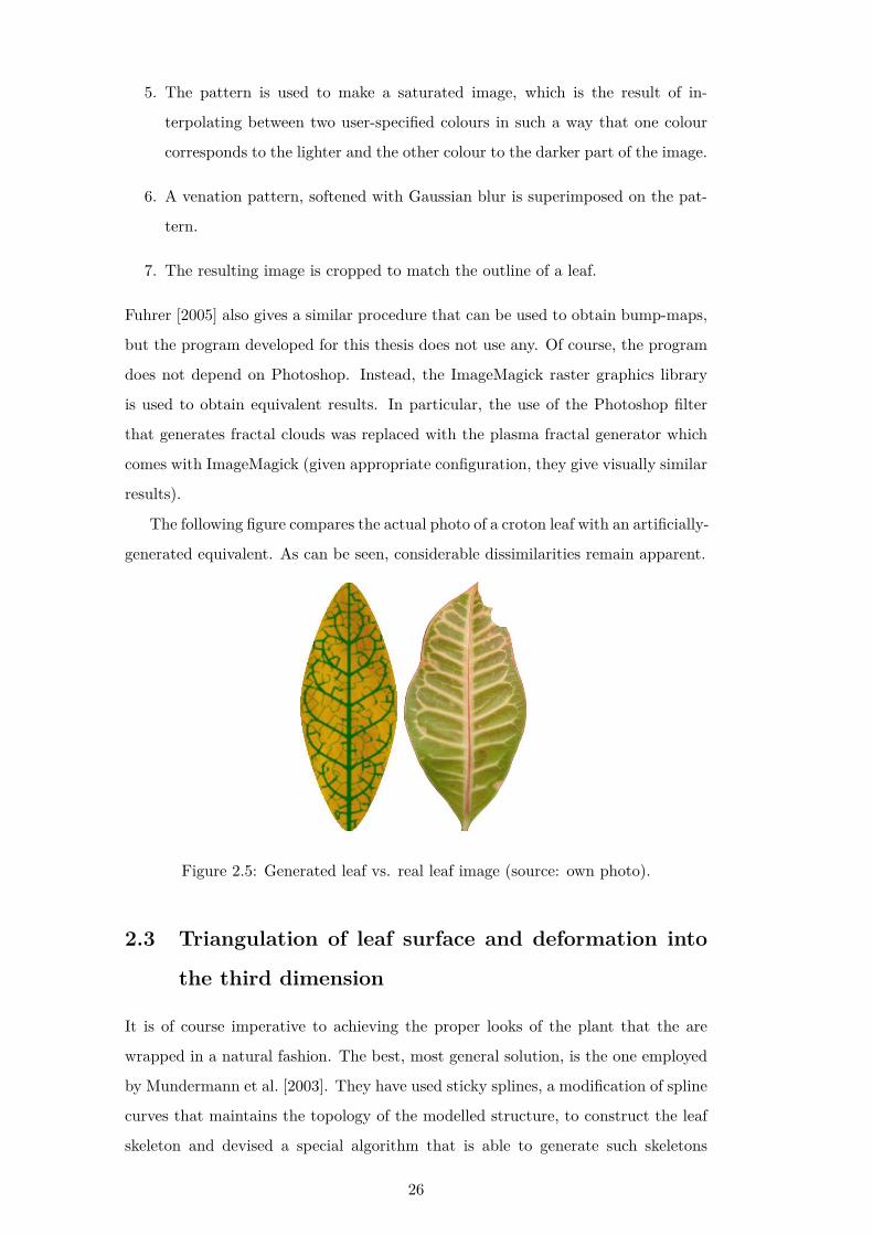
The following figure compares the actual photo of a croton leaf with an artificially-

generated equivalent. As can be seen, considerable dissimilarities remain apparent.

Figure 2.5: Generated leaf vs. real leaf image (source: own photo).

2.3 Triangulation of leaf surface and deformation into

the third dimension

It is of course imperative to achieving the proper looks of the plant that the are

wrapped in a natural fashion. The best, most general solution, is the one employed

by Mundermann et al. [2003]. They have used sticky splines, a modification of spline

curves that maintains the topology of the modelled structure, to construct the leaf

skeleton and devised a special algorithm that is able to generate such skeletons

26

automatically. Naturally, the constructed skeleton corresponds directly to the leaf’s

venation pattern. This allows them to represent arbitrary leaf lobes and thus produce

high-quality renderings of the plants. This approach, however, is both complicated

and computationally expensive, since each primary or secondary leaf vein must be

given its representation in the form of an appropriate spline. Therefore, it is better

suited to plant rendering than to real-time display.

In search of a simpler solution, it became apparent that as long as we do not need

to model leaf deformation that is due to the venation pattern, it suffices to provide

just an arbitrary triangulation of a flat leaf shape, which can then be bent into the

third dimension. It is, however, important that the triangulation is accurate enough

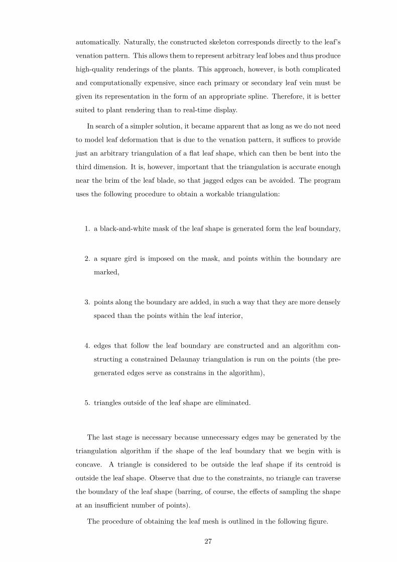
near the brim of the leaf blade, so that jagged edges can be avoided. The program

uses the following procedure to obtain a workable triangulation:

1. a black-and-white mask of the leaf shape is generated form the leaf boundary,

2. a square gird is imposed on the mask, and points within the boundary are

marked,

3. points along the boundary are added, in such a way that they are more densely

spaced than the points within the leaf interior,

4. edges that follow the leaf boundary are constructed and an algorithm con-

structing a constrained Delaunay triangulation is run on the points (the pre-

generated edges serve as constrains in the algorithm),

5. triangles outside of the leaf shape are eliminated.

The last stage is necessary because unnecessary edges may be generated by the

triangulation algorithm if the shape of the leaf boundary that we begin with is

concave. A triangle is considered to be outside the leaf shape if its centroid is

outside the leaf shape. Observe that due to the constraints, no triangle can traverse

the boundary of the leaf shape (barring, of course, the effects of sampling the shape

at an insufficient number of points).

The procedure of obtaining the leaf mesh is outlined in the following figure.

27

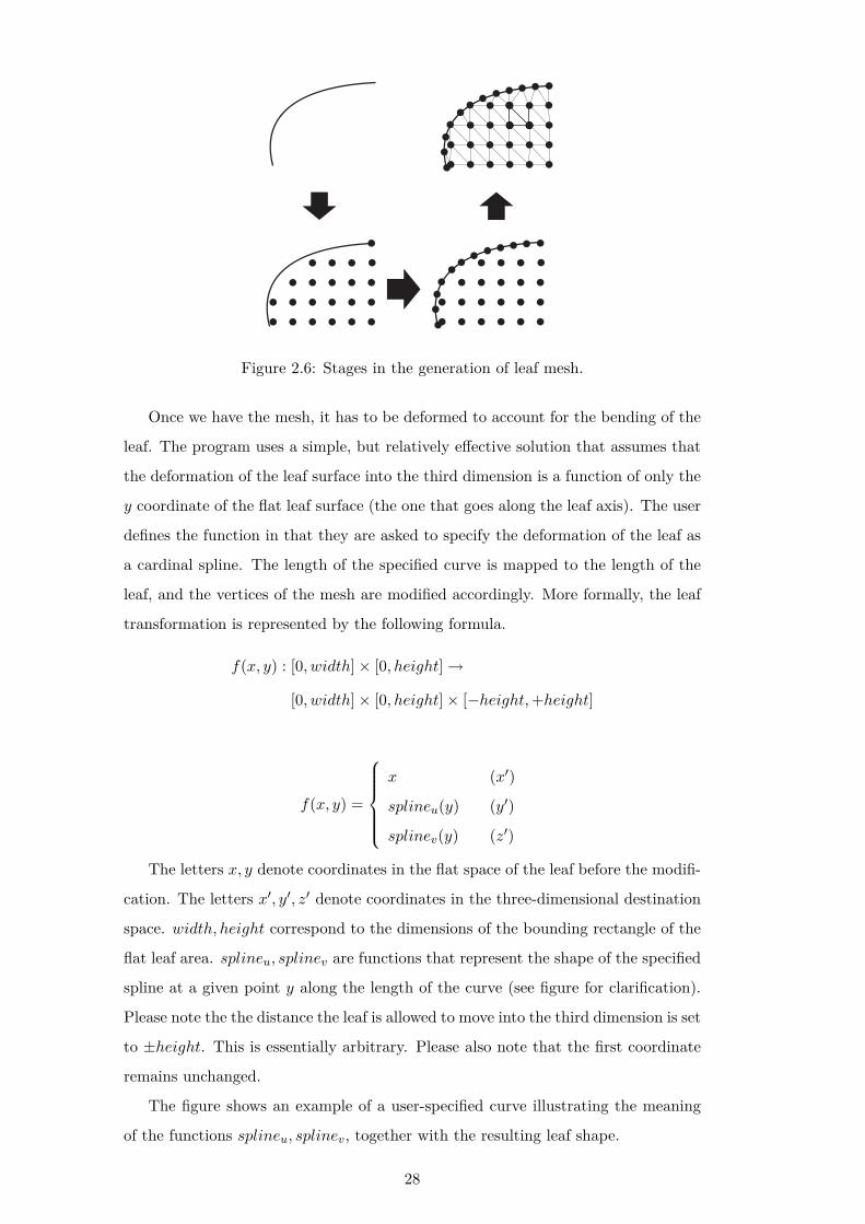
Figure 2.6: Stages in the generation of leaf mesh.

Once we have the mesh, it has to be deformed to account for the bending of the

leaf. The program uses a simple, but relatively effective solution that assumes that

the deformation of the leaf surface into the third dimension is a function of only the

y coordinate of the flat leaf surface (the one that goes along the leaf axis). The user

defines the function in that they are asked to specify the deformation of the leaf as

a cardinal spline. The length of the specified curve is mapped to the length of the

leaf, and the vertices of the mesh are modified accordingly. More formally, the leaf

transformation is represented by the following formula.

f(x, y) : [0, width]× [0, height]→

[0, width]× [0, height]× [−height,+height]

f(x, y) =

x (x′)

splineu(y) (y′)

splinev(y) (z′)

The letters x, y denote coordinates in the flat space of the leaf before the modifi-

cation. The letters x′, y′, z′ denote coordinates in the three-dimensional destination

space. width, height correspond to the dimensions of the bounding rectangle of the

flat leaf area. splineu, splinev are functions that represent the shape of the specified

spline at a given point y along the length of the curve (see figure for clarification).

Please note the the distance the leaf is allowed to move into the third dimension is set

to ±height. This is essentially arbitrary. Please also note that the first coordinate

remains unchanged.

The figure shows an example of a user-specified curve illustrating the meaning

of the functions splineu, splinev, together with the resulting leaf shape.

28

Figure 2.7: The leaf deformation curve (above) and a schematic drawing of a de-

formed leaf (below).

The outlined way of modifying the leaf surface could be extended to achieve more

realistic results by eliminating the indifference of the process to the x coordinate of

the leaf. This would allow the leaf shape to vary with the distance from the leaf axis,

along a second user-specified curve. However, this would most probably still not yield

truly realistic shapes, as long as the displacement due to the two coordinates would

be independent of the other (and if they were dependent, we would get the general

question of how to model an arbitrary surface, which we want to avoid). Another

disadvantage of allowing the user to modify the shape of the leaf in reference to

the x coordinate is that it would have made the prevention of self-intersections more

difficult. Currently, the leaf will self-intersect only if the user-specified curve does so,

which means the user can easily prevent this form happening. It therefore appears

that the best way of achieving a really marked improvement in the results would be

following along the ideas of Mundermann et al. [2003].

2.4 Stem texture

While there seems to have been considerable research into the ways of generating

aesthetically appealing textures of tree bark, I could not find a ready algorithm

specifically geared at reproducing the outer looks of the stems of non-tree plants.

Because devising a new algorithm would be complex, I have opted to use a simple

bark-like pattern that is fast and easy to compute while delivering results of passable

quality. There have been quite a number of different approaches to obtaining the

texture of tree bark:

1. Bloomenthal [1985] used X-rays of real tree bark, which were later post-

processed to make the texture wrap,

2. Oppenheimer [1986] used a noise pattern run through a sawtooth function,

3. Hart and Baker [1996] use a specially-devised particle flow system that gen-

erates a texture for the whole tree in such a way that branching points are

29

properly accounted for,

4. Federl [2003], describes two physically-motivated approaches: the simulation

of mass-spring systems and a finite element algorithm for fracture formation

in stiff materials,

5. Wang et al. [2003] introduced complex software that can be used to gener-

ate photographic-quality bark of all kinds, but is heavily dependent on user

interaction and needs digital images of bark as input.

Because the procedural generation of textures is not the primary focus of the present

thesis, I chose the solution due to Oppenheimer [1986]. His algorithm takes three

inputs: a noise image, an integer N specifying the number of bark ridges and a

real R specifying the roughness of the bark. It generates the output bark texture

according to the following formula:

bark(x, y) = saw (N ∗ (x+R ∗ noise(x, y)))

bark(x, y) : [0, 1]× [0, 1]→ [0, 1]; noise(x, y) : [0, 1]× [0, 1]→ [0, 1]; N ∈ N;R ∈ R+

The sawtooth function is defined as follows:

saw(x) =

2 ∗ fraction(t) if fraction(t) < 0.5

2 ∗ (1− fraction(t)) if fraction(t) ≥ 0.5

It is immediately apparent form the formula that the texture bark wraps in both

dimensions as long as the input noise pattern noise wraps. The question remains

which noise pattern one should use. Oppenheimer [1986] used Brownian fractal

noise, which, however, requires a complex algorithm to compute. For simplicity,

I chose to instead use a fractal noise generator integrated into the ImageMagick

library, called plasma, which is easy to use and delivers acceptable results. Because

the noise generated by ImageMagick does not tile, the noise image is modified in

that four symmetric variants of the same generated image are averaged with equal

weights. Theoretically, this may disturb the properties of the noise, but the visual

effect of such modification on the generated bark is minimal.

The result of the described procedure is a greyscale image. To obtain colour,

the image is saturated using a gradient specified by two user-definable colours. The

first, dominant colour occupies the first half of the gradient, while the second half is

a linear interpolation between the two colours in the RGB colour space.

The following figures demonstrate textures generated using various parameters

30

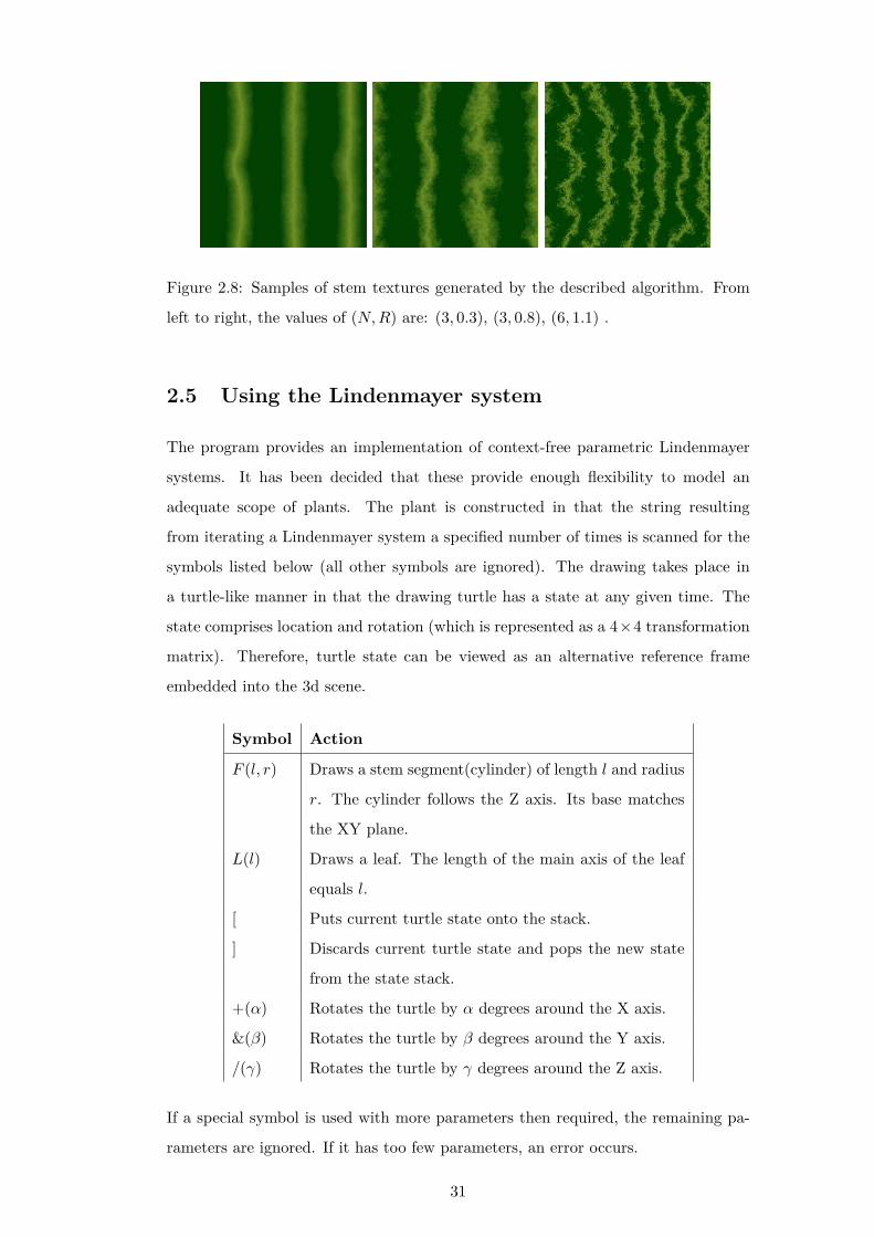
Figure 2.8: Samples of stem textures generated by the described algorithm. From

left to right, the values of (N,R) are: (3, 0.3), (3, 0.8), (6, 1.1) .

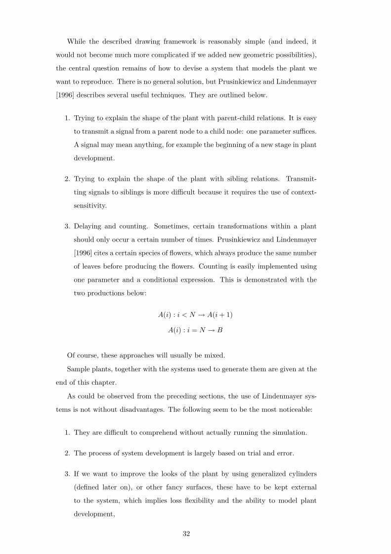
2.5 Using the Lindenmayer system

The program provides an implementation of context-free parametric Lindenmayer

systems. It has been decided that these provide enough flexibility to model an

adequate scope of plants. The plant is constructed in that the string resulting

from iterating a Lindenmayer system a specified number of times is scanned for the

symbols listed below (all other symbols are ignored). The drawing takes place in

a turtle-like manner in that the drawing turtle has a state at any given time. The

state comprises location and rotation (which is represented as a 4×4 transformation

matrix). Therefore, turtle state can be viewed as an alternative reference frame

embedded into the 3d scene.

Symbol Action

F (l, r) Draws a stem segment(cylinder) of length l and radius

r. The cylinder follows the Z axis. Its base matches

the XY plane.

L(l) Draws a leaf. The length of the main axis of the leaf

equals l.

[ Puts current turtle state onto the stack.

] Discards current turtle state and pops the new state

from the state stack.

+(α) Rotates the turtle by α degrees around the X axis.

&(β) Rotates the turtle by β degrees around the Y axis.

/(γ) Rotates the turtle by γ degrees around the Z axis.

If a special symbol is used with more parameters then required, the remaining pa-

rameters are ignored. If it has too few parameters, an error occurs.

31

While the described drawing framework is reasonably simple (and indeed, it

would not become much more complicated if we added new geometric possibilities),

the central question remains of how to devise a system that models the plant we

want to reproduce. There is no general solution, but Prusinkiewicz and Lindenmayer

[1996] describes several useful techniques. They are outlined below.

1. Trying to explain the shape of the plant with parent-child relations. It is easy

to transmit a signal from a parent node to a child node: one parameter suffices.

A signal may mean anything, for example the beginning of a new stage in plant

development.

2. Trying to explain the shape of the plant with sibling relations. Transmit-

ting signals to siblings is more difficult because it requires the use of context-

sensitivity.

3. Delaying and counting. Sometimes, certain transformations within a plant

should only occur a certain number of times. Prusinkiewicz and Lindenmayer

[1996] cites a certain species of flowers, which always produce the same number

of leaves before producing the flowers. Counting is easily implemented using

one parameter and a conditional expression. This is demonstrated with the

two productions below:

A(i) : i < N → A(i+ 1)

A(i) : i = N → B

Of course, these approaches will usually be mixed.

Sample plants, together with the systems used to generate them are given at the

end of this chapter.

As could be observed from the preceding sections, the use of Lindenmayer sys-

tems is not without disadvantages. The following seem to be the most noticeable:

1. They are difficult to comprehend without actually running the simulation.

2. The process of system development is largely based on trial and error.

3. If we want to improve the looks of the plant by using generalized cylinders

(defined later on), or other fancy surfaces, these have to be kept external

to the system, which implies loss flexibility and the ability to model plant

development,

32

4. Beyond what has been described in the first chapter, they are not easily ex-

tensible in a way that would be beneficial to their use as a tool for modelling

plants.

However, they do not appear to have a reasonable alternative. All other solutions

the author of the thesis is aware of either boil down to using an artist to model plant

shape with of predefined surfaces or to the processing of photos of real plants. This

goes against the main idea of the present thesis, which is to keep the approach

as procedural as possible. In fact, the only aspects of the plant that are directly

controlled by the user are: the leaf shape, veins initially put on the leaf, and leaf

deformation.

2.6 Modelling the shape of the plant’s stem

The issue of how to model a plant’s stem so as to achieve adequate results is a

difficult one because optically-pleasing solutions usually require complex algorithms

to generate the mesh. The problem can be divided into two separate issues:

1. The modelling of a single separate segment of the branch.

Bloomenthal [1985] used the notion of generalised cylinder to model the maple.

He defined it as a surface generated by sweeping a disk along a spline curve, but

others have later extended the definition by using another spline (or any other

curve) instead of a disk. The curve must not necessarily be closed and may

change along the sweep length. Snyder and Kajiya [1992] delivered a formal

analysis of the general case of applying operators from a pre-specified set to

arbitrary continuous partially differentiable functions as a way of modelling

any object. Generalised cylinders are special cases where the sweep operator is

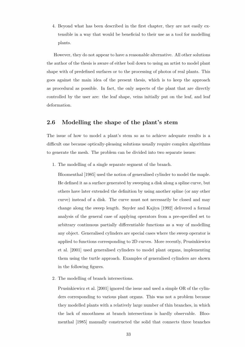
applied to functions corresponding to 2D curves. More recently, Prusinkiewicz

et al. [2001] used generalised cylinders to model plant organs, implementing

them using the turtle approach. Examples of generalised cylinders are shown

in the following figures.

2. The modelling of branch intersections.

Prusinkiewicz et al. [2001] ignored the issue and used a simple OR of the cylin-

ders corresponding to various plant organs. This was not a problem because

they modelled plants with a relatively large number of thin branches, in which

the lack of smoothness at branch intersections is hardly observable. Bloo-

menthal [1985] manually constructed the solid that connects three branches

33

Figure 2.9: Examples of generalised cylinders.

from surface that span along splines. This had the implication that only three

branches were allowed to meet at a given point, which may not have been

an issue with modelling the maple, which was what he tried to do, but may

constitute a considerable obstacle in modelling other plants. Bloomenthal and

Wyvill [1990] use skeletons to model surfaces, and provide a blend of general-

ized cylinders (albeit with fixed radius) as an example. Hart and Baker [1996]

extended this approach to account for the blending of cones.

Whatever the advantages of generalised cylinders may be, they severely compli-

cate the generation of the plant with Lindenmayer Systems. Prusinkiewicz et al.

[2001] uses additional, predefined functions that are external to the system to in-

tegrate the cylinders into their modelling framework. One might argue that this

undermines the primary motivation of using Lindenmayer systems in the fist place,

which is the fact that they work best when applied to the whole process of plant

modelling. If they are not, we lose the ability to exploit them where they have the

greatest potential: in the adaptation of ordinary plant models to account for plant

growth and variations within specimens of the same plant species.

For lack of time, and because of the said difficulties in integrating generalised

cylinders into an application based on Lindenmayer systems, it has been necessary

to give up the use of these fancy algorithms to model the stem. Ordinary (not

generalised) cylinders have been used as a replacement.

2.7 Possibilities of further development

As could be concluded from the preceding sections, almost every aspect of the plant

could be improved on. The list of possible improvements that are most adequate is

presented below.

1. Account for leaf growth in the generation of venation pattern.

This would possibly reduce the reliance on manually pre-set vein configurations

34

as well as allow the user to try out different combinations of leaf shapes and

growth types.

2. Use a morphologically-motivated triangulation of leaf surface.

This would allow for easy modelling of leaf lobes adding another dimension

to the model. It would also reduce the reliance on pre-set leaf deformation

patterns as the degree to which the leaf is lobed and the kind of lobes could be

controlled with additional parameters of tokens in the Lindenmayer system.

3. Find a better algorithm to reproduce stem texture.

The present algorithm is hardly satisfactory. It is a tree bark algorithm and

it models, well, tree bark. While there exists some visual correlation between

tree bark and stem texture, it is vague at best.

4. Apply generalized cylinders to the modelling of plant stem, possibly with

blending.

The current use of ordinary cylinders makes branch intersections very rigid.

Also, branch segments are currently straight, which means the whole plant

has an unnatural look. They are textured independently, which means vi-

sual artefacts appear in places where they meet. A comprehensive modelling

framework based on generalized cylinders would resolve these problems.

5. Prevent self-intersections

The current implementation of both leaf deformation and Lindenmayer system

does not prevent self-intersection. This may be a problem because sometimes

such self-intersections severely deteriorate the plant’s appearance. However,

the only method the author of the thesis is aware of would be a division of

the three dimensional space into tiny cubes and checking whether more than

one primitive contains the centre point of each cube. This would be very slow.

It appears to be very difficult to detect self-intersections in the productions

specifying the Lindenmayer system, without actually iterating it the required

number of steps.

2.8 Sample plants

1. The following system, heavily adapted from Prusinkiewicz and Lindenmayer

[1996], has been used (the system is given in the form used by the program).

35

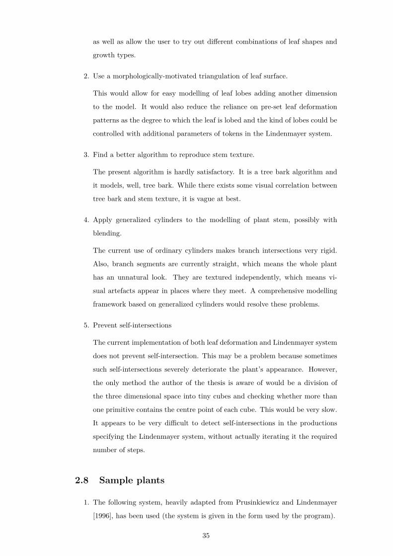
axiom -> A(100,5,200)

A(s,t,l) -> [&(22.5)F(s,t,l)L(l)A(s,t/2 + 2,l)] /(5*22.5)

[&(22.5)F(s,t,l)L(l)A(s,t/2 + 2,l)] /(7*22.5)

[&(22.5)F(s,t,l)L(l)A(s,t/2 + 2,l)]

F(s,t,l) -> S(t,s,l) /(5*22.5) F(s,t,l)

S(s,t,l) -> F(t,s,l)

Figure 2.10: Plant generated from the system above (3 iterations).

The way the system works is centred around the A token. This token has three

parameters, which stand for the following: the length of a single stem segment,

the width of the stem segment and the length of the leaf. In each iteration,

the A token produces three branches using the [ and ] stack operators. They

protrude from their base at different angles (the / operator). Each branch

consists of an appropriately rotated (&) stem segment (F), a leaf (L) and the

token A which allows it to split further and form child branches in subsequent

iterations. Note how the stem width is decreased as the plant grows. It

is guaranteed to be at least 2 so that the stem remains visible. Note also

how the last two productions account for the growth of already-formed stem

segments. When this production is used, the segments will already have been

in the model for at least one iteration, they are therefore ”older” and thus

need to be more pronounced. Also, the production introduces the rotation

around the central axis to prevent the resulting structure form appearing too

symmetrical.

2. Below is presented a system that reproduces a yucca plant

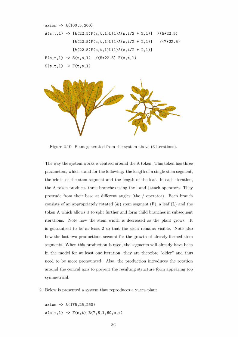
axiom -> A(175,25,250)

A(s,t,l) -> F(s,t) B(7,6,l,60,s,t)

36

B(h,v,l,d,s,t) -> BN(h,v,v,l,d,s,t)

BN(h,v,i,l,d,s,t) -> LR(h,l,d*v/i) /(13) F(s/10,t) BN(h-0.4,v-1,i,l,d,s/2,t)

LR(n,l,d) -> LRN(n,n,l,d)

LRN(i,n,l,d): i == 0 -> eps

LRN(i,n,l,d): i > 0 -> [+(d)L(l)] /(360/n) LRN(i-1,n,l,d)

Figure 2.11: A real yucca photo (source: www.pyraflora.co.za) together with models

generated with 100 (centre) and 10 (right) iterations of the system above.

This model was been inspired by a photo of a real yucca plant. First, look at

the last three productions below: they represent a ”procedure” ”invoked” by

using the LR(n,l,d) token. It draws n uniformly distributed leaves of length

n and inclination d. The two productions from B and BN generate a num-

ber of such concentric leaf groups (once group is added for one iteration). The

parameters of the leafs are varied to achieve a less symmetrical look. In partic-

ular the inclination change reproduces the dome-like shape of the whole plant.

After each group of leaves has been drawn, the coordinate system is rotated so

that the leaves of the next group do not protrude from the plant at the same

angles. Also, a short stem segment is added. The token A is used to add the

first, long stem segment and initiate the generation process.

3. This system reproduces a fern leaf. It is a heavily modified version of a system

proposed by Prusinkiewicz and Lindenmayer [1996].

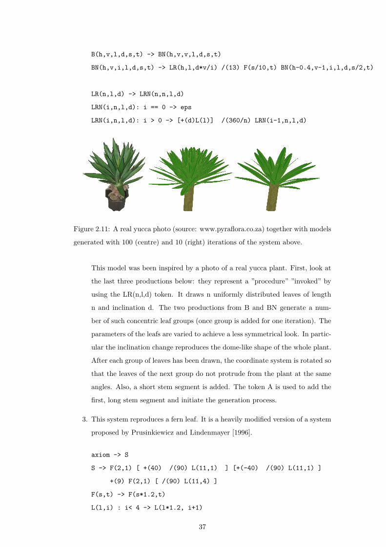
axiom -> S

S -> F(2,1) [ +(40) /(90) L(11,1) ] [+(-40) /(90) L(11,1) ]

+(9) F(2,1) [ /(90) L(11,4) ]

F(s,t) -> F(s*1.2,t)

L(l,i) : i< 4 -> L(l*1.2, i+1)

37

L(l,i) : i==4 -> [ / (270) S ]

Figure 2.12: A real fern photo (source: Wikipedia) together with a generated model

(20 iterations).

The basic idea of this system is based on the fractal-like structure of a fern

leaf, where smaller elements have the same structure as larger elements. The

basic building block of the fern leaf is represented with the production from S:

two branches (L) protrude from a stem made from to segments. The rotation

before drawing the leaves is necessary so that the surface of the leaves is aligned

with the surface of the whole leaf. The rotation +(9) before the creation of

the second stem segment is used to make the whole leaf bend. Note how

the L symbol, whose main purpose is the creation of leaves is used to create

branches. Its second parameter is used in a timer, which converts the leaf to

the basic building block after a fixed number of iterations (this is done .using

the two last productions). This way, the youngest generation of created objects

is rendered in the form of leaves. The disadvantage is that this has absolutely

no biological motivation, but it looks good enough. The production from F is

used to elongate the existing stem segments so there is enough place for the

emergence of new ones in the following iteration steps.

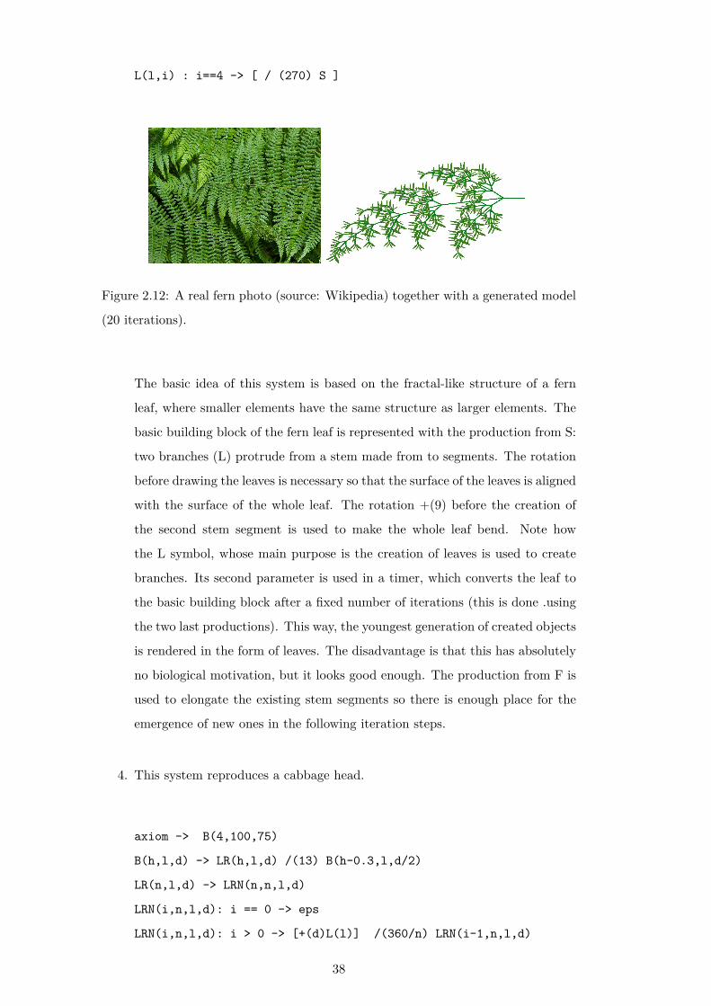
4. This system reproduces a cabbage head.

axiom -> B(4,100,75)

B(h,l,d) -> LR(h,l,d) /(13) B(h-0.3,l,d/2)

LR(n,l,d) -> LRN(n,n,l,d)

LRN(i,n,l,d): i == 0 -> eps

LRN(i,n,l,d): i > 0 -> [+(d)L(l)] /(360/n) LRN(i-1,n,l,d)

38

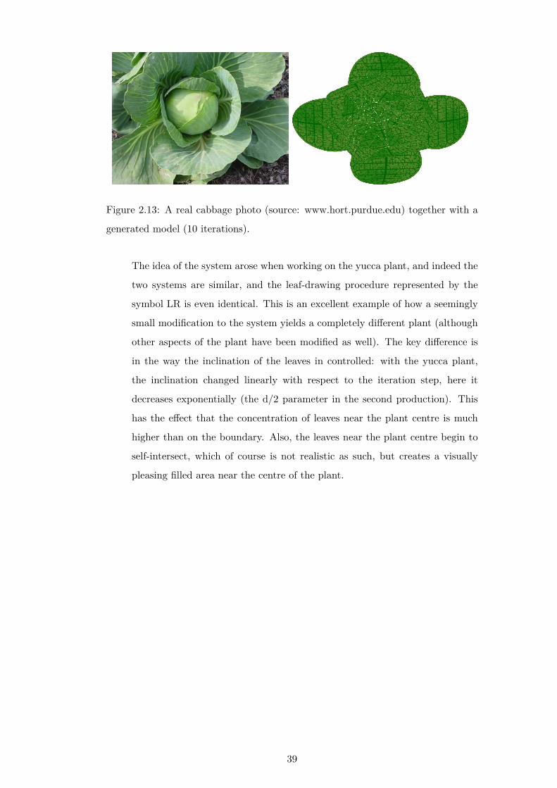
Figure 2.13: A real cabbage photo (source: www.hort.purdue.edu) together with a

generated model (10 iterations).

The idea of the system arose when working on the yucca plant, and indeed the

two systems are similar, and the leaf-drawing procedure represented by the

symbol LR is even identical. This is an excellent example of how a seemingly

small modification to the system yields a completely different plant (although

other aspects of the plant have been modified as well). The key difference is

in the way the inclination of the leaves in controlled: with the yucca plant,

the inclination changed linearly with respect to the iteration step, here it

decreases exponentially (the d/2 parameter in the second production). This

has the effect that the concentration of leaves near the plant centre is much

higher than on the boundary. Also, the leaves near the plant centre begin to

self-intersect, which of course is not realistic as such, but creates a visually

pleasing filled area near the centre of the plant.

39

40

Chapter 3

Implementation

This chapter summarizes technical decisions taken during the development of the

program accompanying this thesis.

3.1 The choice of the technology

It was immediately obvious that the program had to be implemented in a managed

language to facilitate its primary function a test field for algorithms. Managed lan-

guages make it easy to create flexible designs at the cost of code speed. However,

code speed is not that important while researching algorithms. In fact, it turned

out that the program runs quite fast (less than one minute for the most complicated

algorithm, generating the venation pattern of the leaf). Also, IDE automation (sup-

port for refactoring, unit testing etc.) is better with managed languages. Therefore,

there remained the following choices:

1. Sun Java

2. Microsoft C# / .NET

3. Adobe Flex

It has been decided to use the C# language (version 2.0). This decision was made

because of easy interoperation with unmanaged code (the program uses external

unmanaged libraries, which do not have ready bindings for any of the said solutions),

because the tools for user interface design are better as well as because Microsoft

delivers a ready Managed DirectX component, which seems to be easier to use than

the Java3D API delivered by Sun.

Of course, the main difficulty of this thesis is in the assembly of the toolchain

algorithms, which is essentially independent of the choice of language, so most prob-

41

ably any of the said solutions would work well enough.

3.2 The design and structure of the program

The program has a modular architecture, which means that modifications to the way

various aspects of the program are implemented can be done in a way independent of

one another. The following list gives a brief description of each module and presents

the most important implementation decisions take during its development.

1. The toolchain controls

The program consists of several controls, each responsible for a stage of the

toolchain described in the previous chapter. They include controls for: design-

ing leaf shape, designing leaf veins, specifying leaf deformation, leaf texture,

stem texture and the Lindenmayer System. These controls are not created

each the user invokes a given option, but only once, during the initialization

of the program. This allows for a more responsive interface.

2. Data module.

This module serves as a central database of the aspect of the plant that a user

can modify. The data module maintains a collection of the toolchain controls

and enables each part of the program to access data stored in other parts.

For example, the algorithm that generates plant mesh once the user clicks

the View Plant button has to access, among others, the stem texture, which

is stored in an object of type StemTextureGeneratorControl. To do this, it

simply retrieves a reference to the control responsible for the texture from this

central database. This is done like this:

[C#]

StemTextureGeneratorControl stcg = (StemTextureGeneratorControl)

ComponentStorage.Instance.GetControl(

typeof(StemTextureGeneratorControl)))

In this code, the static property ComponentStorage.Instance returns the one

and only object that holds references to the stored data. Please note that the

design idea of having all data in the same place, and accessible through a fixed

interface has the added benefit of making it very easy to save plants to files.

Moreover, it makes it easy to support the possibility that the user cancelled

the changes done in the control. This is not trivial, because these changes may

42

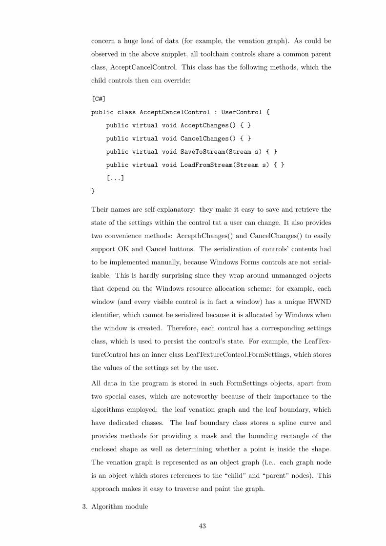
concern a huge load of data (for example, the venation graph). As could be

observed in the above snipplet, all toolchain controls share a common parent

class, AcceptCancelControl. This class has the following methods, which the

child controls then can override:

[C#]

public class AcceptCancelControl : UserControl {

public virtual void AcceptChanges() { }

public virtual void CancelChanges() { }

public virtual void SaveToStream(Stream s) { }

public virtual void LoadFromStream(Stream s) { }

[...]

}

Their names are self-explanatory: they make it easy to save and retrieve the

state of the settings within the control tat a user can change. It also provides

two convenience methods: AccepthChanges() and CancelChanges() to easily

support OK and Cancel buttons. The serialization of controls’ contents had

to be implemented manually, because Windows Forms controls are not serial-

izable. This is hardly surprising since they wrap around unmanaged objects

that depend on the Windows resource allocation scheme: for example, each

window (and every visible control is in fact a window) has a unique HWND

identifier, which cannot be serialized because it is allocated by Windows when

the window is created. Therefore, each control has a corresponding settings

class, which is used to persist the control’s state. For example, the LeafTex-

tureControl has an inner class LeafTextureControl.FormSettings, which stores

the values of the settings set by the user.

All data in the program is stored in such FormSettings objects, apart from

two special cases, which are noteworthy because of their importance to the

algorithms employed: the leaf venation graph and the leaf boundary, which

have dedicated classes. The leaf boundary class stores a spline curve and

provides methods for providing a mask and the bounding rectangle of the

enclosed shape as well as determining whether a point is inside the shape.

The venation graph is represented as an object graph (i.e.. each graph node

is an object which stores references to the “child” and “parent” nodes). This

approach makes it easy to traverse and paint the graph.

3. Algorithm module

43

This module provides an implementation of the algorithms described in the

previous chapter. Only the non-trivial aspects of the implementation are dis-

cussed here.

In the algorithm that generates the venation pattern, a data structure was

needed to account for the tagging of sources that have been reached by one,

but not all nodes. This structure had to support the basic operations listed

below.

(a) Insertion of a pair (vein node, source). This is needed when the nodes

are tagged.

(b) Removal of a pair (vein node, source). This is needed when a node reaches

the source, or ventures too far from the source.

(c) Retrieval of all pairs contacting a given vein node. This is needed to

update the tags when the vein grows.

(d) Retrieval of all pairs containing a given source. This is needed to check

if the source should be deleted.

This interface directly corresponds to a simple database-table. Therefore, a

.NET DataTable has been used to sore the tags. Please note that, in addition

to the said structure, a set is required to hold the sources which are considered

for deletion to implement the tagging. This is because if no pair with a given

source exists in the table, it may both mean that no nodes have yet reached

it, or that every node that could have reached it has already done so.

In the algorithm that generates the leaf texture, a mix of Windows GDI+ and

ImageMagick APIs has been used. GDI+ is used to generate the initial vein

pattern and for clipping, while ImageMagick is used to generate the leaf back-

ground and blend it with the veins. This combination allows the program to

profit from the advantages of both solutions, which is the ability to easily draw

geometric primitives for GDI+ and the ability to quickly complete expensive

raster operations for ImageMagick.

4. Parsing Lindenmayer Systems

A simple Lindenmayer system parser has been written with the help of the

GPLEX lexer for C#. Parsing context-free parametric Lindenmayer systems

is simple, apart from the evaluation of arithmetic expressions and conditions.

It turned out that there is a simpler solution of doing this than using a parser

44

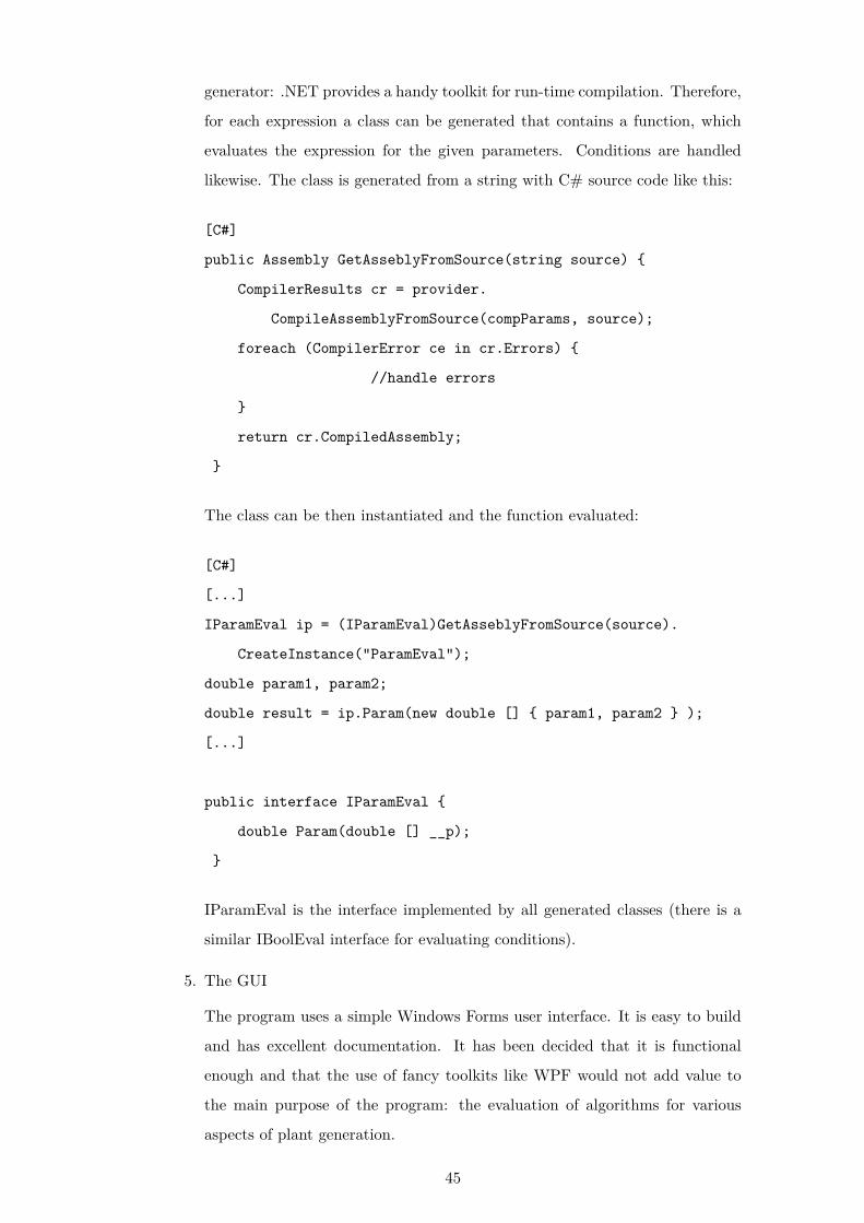
generator: .NET provides a handy toolkit for run-time compilation. Therefore,

for each expression a class can be generated that contains a function, which

evaluates the expression for the given parameters. Conditions are handled

likewise. The class is generated from a string with C# source code like this:

[C#]

public Assembly GetAsseblyFromSource(string source) {

CompilerResults cr = provider.

CompileAssemblyFromSource(compParams, source);

foreach (CompilerError ce in cr.Errors) {

//handle errors

}

return cr.CompiledAssembly;

}

The class can be then instantiated and the function evaluated:

[C#]

[...]

IParamEval ip = (IParamEval)GetAsseblyFromSource(source).

CreateInstance("ParamEval");

double param1, param2;

double result = ip.Param(new double [] { param1, param2 } );

[...]

public interface IParamEval {

double Param(double [] __p);

}

IParamEval is the interface implemented by all generated classes (there is a

similar IBoolEval interface for evaluating conditions).

5. The GUI

The program uses a simple Windows Forms user interface. It is easy to build

and has excellent documentation. It has been decided that it is functional

enough and that the use of fancy toolkits like WPF would not add value to

the main purpose of the program: the evaluation of algorithms for various

aspects of plant generation.

45

6. Visualization with DirectX

Although the author of this thesis has a personal preference for OpenGL,

it has been decided to use DirectX as a foundation for the 3D visualization

control because Microsoft provides reasonably complete bindings in the form

of a ready component, which is a part (albeit an optional one), of the popular

DirectX distribution. Unfortunately, it was necessary to stick with the obsolete

Managed DirectX 1.1, because the new 2.0 version was abandoned by Microsoft

in favour of the XNA technology.

To render the plant, the following features of DirectX have been used:

(a) Leaves are represented with Mesh objects, which are created from trian-

gles obtained in the way described in the toolchain section. Of course, the

triangles are adorned with texture coordinate information beforehand.

(b) Stem segments (cylinders) are also represented by Mesh objects, but they

are created by DirectX’s internal facility for creating 3D primitives. Tex-

ture wrapping in the horizontal dimension is applied during the mapping

of stem texture onto the cylinder to achieve continuous visual appearance.

The objects can then be displayed either as wireframe skeletons, or as solids

only lit with ambient light.

3.3 The use of external libraries

During the work on this thesis, it has been decided that some portions of work need

to be “outsourced” to external libraries. This saved both development time, allowing

more to be spent on the actual study of generating the plant. Also, external libraries

save computation time, because they are implemented unmanaged code, and usually

in a highly optimal way.

The following two libraries have been used.

1. CGAL

This library provides excellent routines for computing unconstrained and con-

strained Delaunay triangulations of arbitrary point sets. It makes heavy use

of template metaprogramming and is thus very fast. In fact, the program

only uses a fraction of the capabilities that this library offers. Also, it is very

extensible. For example, in the process of writing the program, it became

apparent that the points being triangulated needed to be give unique indices.

46

The library was designed well enough that it provided the option of inserting

a custom point class, which solved the problem.

While the way it is used to triangulate point sets is quite straightforward,

it deserves a mention how Urquhart triangulation was obtained. The follow-

ing code stores the indices of points incident to point (x, y) in an Urquhart

triangulation of set S ∪ {(x, y)}, where S is a set of points that has already

been triangulated once this function is run. To avoid cluttering the code with

unnecessary details, a simplified version of the code is printed.

[pseudocode adapted from C++]

//Delaunay triangulation, already contains some points

Triangulation T;

void InsertPoint(int x, int y) {

vector adjacentPoints;

PointHandle ph = T.Insert(new Point (x,y) );

foreach (PointHandle p adjacent to ph in T) {

if (IncludeEdge(previous(p), p, next(p), ph))

adjacentPoints.Add(p);

}

T.Remove(ph);

}

bool IncludeEdge(PointHandle left, PointHandle x,

PointHandle r, PointHandle np);

The function IncludeEdge() returns false if (np, x) is the longest edge of the

triangle (np, x, left) or (np, x, right), otherwise it returns true. Therefore, we

only add those vertices adjacent to the new vertex in a Delaunay triangulation,

which are also adjacent to it in the Urquhart triangulation. The reason for

this is explained in greater detail in the first chapter.

The used version of CGAL was 3.3.1, the most recent at the time of writing

the program.

2. ImageMagick

This library facilitates fast processing of raster images. The following features

of the library were used: plasma generator (generates an image of fractal

47

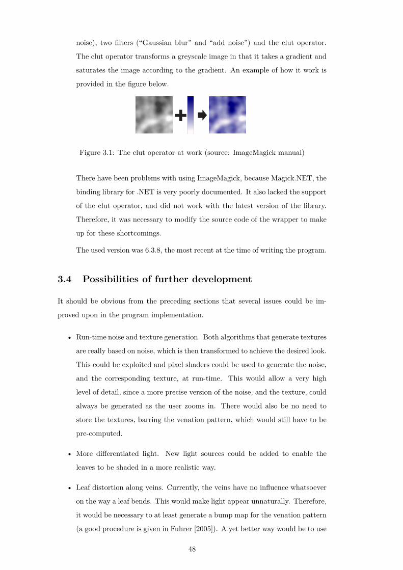
noise), two filters (“Gaussian blur” and “add noise”) and the clut operator.

The clut operator transforms a greyscale image in that it takes a gradient and

saturates the image according to the gradient. An example of how it work is

provided in the figure below.

Figure 3.1: The clut operator at work (source: ImageMagick manual)

There have been problems with using ImageMagick, because Magick.NET, the

binding library for .NET is very poorly documented. It also lacked the support

of the clut operator, and did not work with the latest version of the library.

Therefore, it was necessary to modify the source code of the wrapper to make

up for these shortcomings.

The used version was 6.3.8, the most recent at the time of writing the program.

3.4 Possibilities of further development

It should be obvious from the preceding sections that several issues could be im-

proved upon in the program implementation.

• Run-time noise and texture generation. Both algorithms that generate textures

are really based on noise, which is then transformed to achieve the desired look.

This could be exploited and pixel shaders could be used to generate the noise,

and the corresponding texture, at run-time. This would allow a very high

level of detail, since a more precise version of the noise, and the texture, could

always be generated as the user zooms in. There would also be no need to

store the textures, barring the venation pattern, which would still have to be

pre-computed.

• More differentiated light. New light sources could be added to enable the

leaves to be shaded in a more realistic way.

• Leaf distortion along veins. Currently, the veins have no influence whatsoever

on the way a leaf bends. This would make light appear unnaturally. Therefore,

it would be necessary to at least generate a bump map for the venation pattern

(a good procedure is given in Fuhrer [2005]). A yet better way would be to use

48

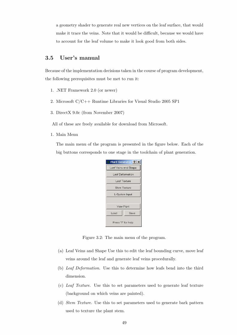
a geometry shader to generate real new vertices on the leaf surface, that would

make it trace the veins. Note that it would be difficult, because we would have

to account for the leaf volume to make it look good from both sides.

3.5 User’s manual

Because of the implementation decisions taken in the course of program development,

the following prerequisites must be met to run it:

1. .NET Framework 2.0 (or newer)

2. Microsoft C/C++ Runtime Libraries for Visual Studio 2005 SP1

3. DirectX 9.0c (from November 2007)

All of these are freely available for download from Microsoft.

1. Main Menu

The main menu of the program is presented in the figure below. Each of the

big buttons corresponds to one stage in the toolchain of plant generation.

Figure 3.2: The main menu of the program.

(a) Leaf Veins and Shape Use this to edit the leaf bounding curve, move leaf

veins around the leaf and generate leaf veins procedurally.

(b) Leaf Deformation. Use this to determine how leafs bend into the third

dimension.

(c) Leaf Texture. Use this to set parameters used to generate leaf texture

(background on which veins are painted).

(d) Stem Texture. Use this to set parameters used to generate bark pattern

used to texture the plant stem.

49

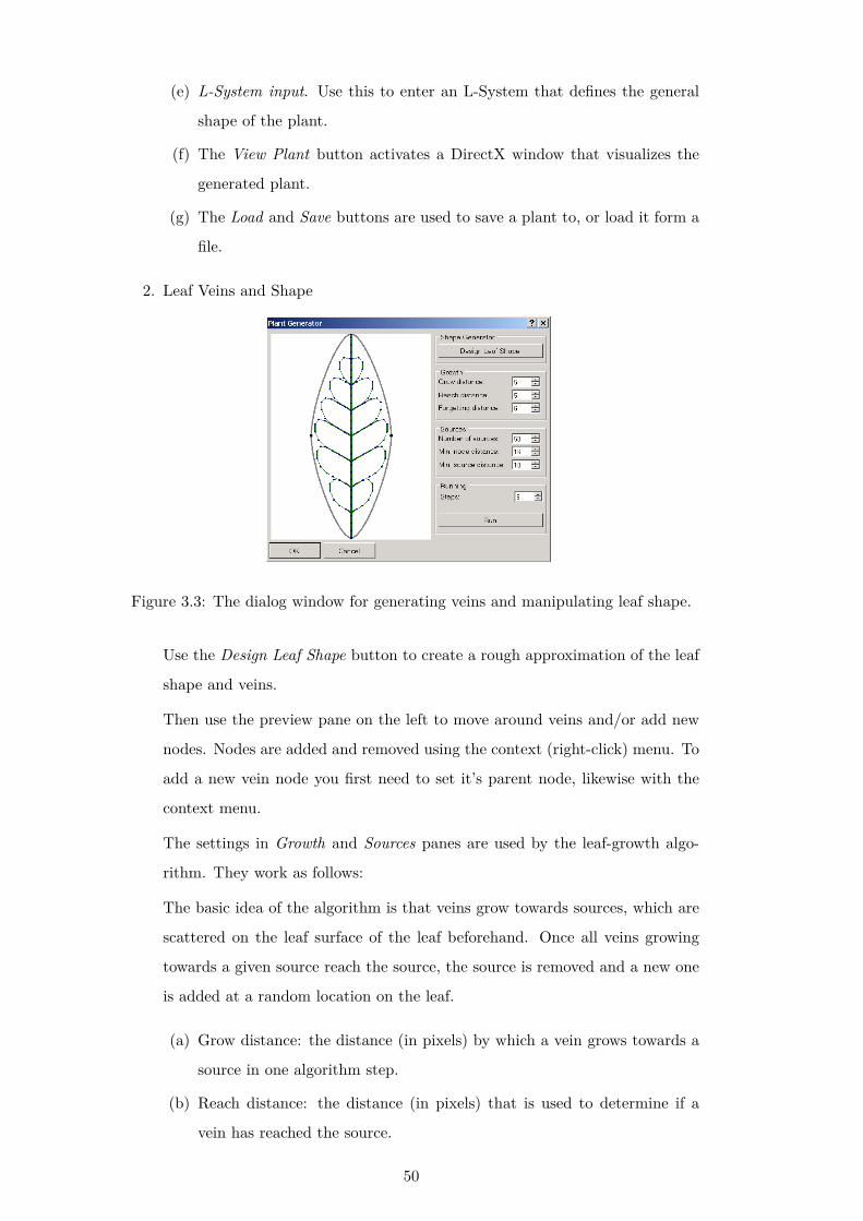
(e) L-System input. Use this to enter an L-System that defines the general

shape of the plant.

(f) The View Plant button activates a DirectX window that visualizes the

generated plant.

(g) The Load and Save buttons are used to save a plant to, or load it form a

file.

2. Leaf Veins and Shape

Figure 3.3: The dialog window for generating veins and manipulating leaf shape.

Use the Design Leaf Shape button to create a rough approximation of the leaf

shape and veins.

Then use the preview pane on the left to move around veins and/or add new

nodes. Nodes are added and removed using the context (right-click) menu. To

add a new vein node you first need to set it’s parent node, likewise with the

context menu.

The settings in Growth and Sources panes are used by the leaf-growth algo-

rithm. They work as follows:

The basic idea of the algorithm is that veins grow towards sources, which are

scattered on the leaf surface of the leaf beforehand. Once all veins growing

towards a given source reach the source, the source is removed and a new one

is added at a random location on the leaf.

(a) Grow distance: the distance (in pixels) by which a vein grows towards a

source in one algorithm step.

(b) Reach distance: the distance (in pixels) that is used to determine if a

vein has reached the source.

50

(c) Forgetting distance: nodes that have moved further than the forgetting

distance from a source are considered irrelevant to the source. Therefore,

they source may be removed even if they have not reached it.

(d) Number of sources: the initial number of sources scattered on the leaf

surface. If it is too large, and it is impossible to scatter the sources in

a way that satisfies the constrains set by 5. and 6., a smaller number of

sources is used.

(e) Minimum node distance: the minimum distance from a newly-added

source to existing vein nodes.

(f) Minimum source distance: the minimum distance from a newly-added

source to existing sources.

(g) The Run Button starts the vein-growing algorithm.

(h) The number of steps is determined with the Steps setting.

3. Leaf Shape Designer

Figure 3.4: The dialog used set leaf shape and initial vein loops.

Use the leaf display to modify a curve that bounds the leaf surface.

Drag points to edit curve. Double-click to add new curve points. Right-click

to delete points.

The set the following options that specify the way the inner vein loops are

generated.

(a) Node distance: the resolution of the loops. The smaller the distance, the

more nodes are added.

(b) Loop number: the number of vein loops that the program tries to add.

A loop will not be added if it does not fit into the bounding curve.

51

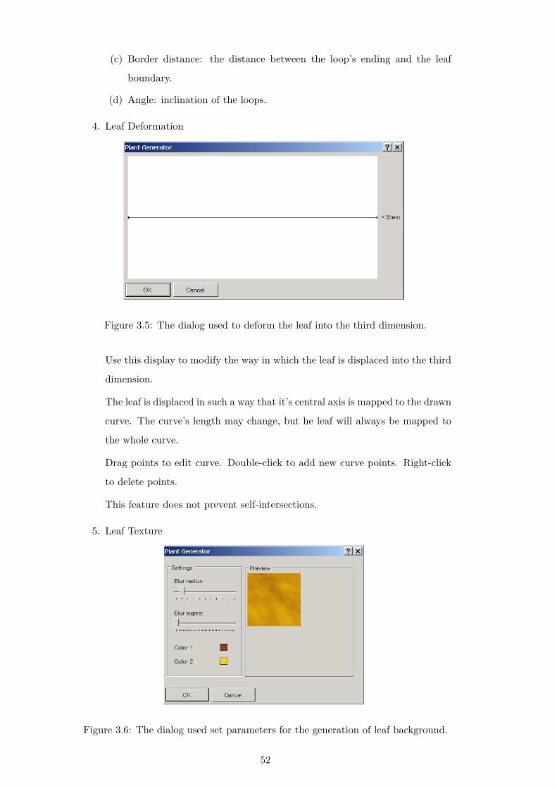
(c) Border distance: the distance between the loop’s ending and the leaf

boundary.

(d) Angle: inclination of the loops.

4. Leaf Deformation

Figure 3.5: The dialog used to deform the leaf into the third dimension.

Use this display to modify the way in which the leaf is displaced into the third

dimension.

The leaf is displaced in such a way that it’s central axis is mapped to the drawn

curve. The curve’s length may change, but he leaf will always be mapped to

the whole curve.

Drag points to edit curve. Double-click to add new curve points. Right-click

to delete points.

This feature does not prevent self-intersections.

5. Leaf Texture

Figure 3.6: The dialog used set parameters for the generation of leaf background.

52

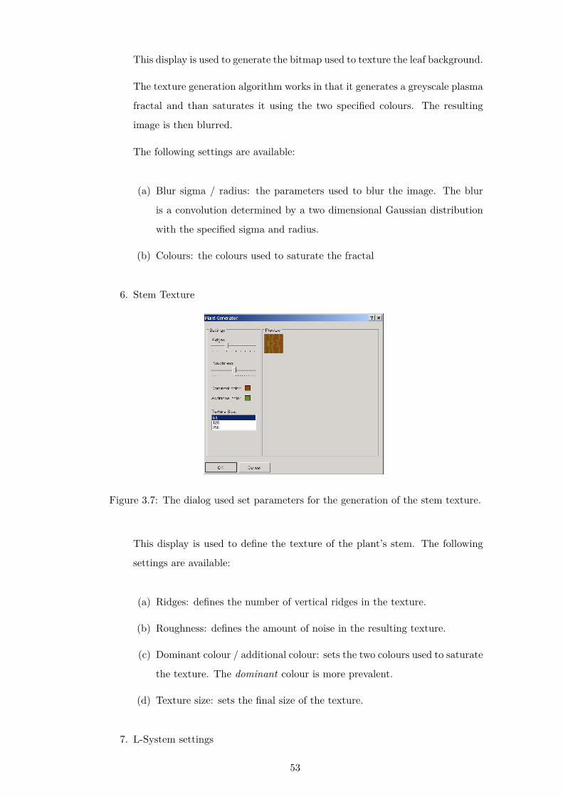
This display is used to generate the bitmap used to texture the leaf background.

The texture generation algorithm works in that it generates a greyscale plasma

fractal and than saturates it using the two specified colours. The resulting

image is then blurred.

The following settings are available:

(a) Blur sigma / radius: the parameters used to blur the image. The blur

is a convolution determined by a two dimensional Gaussian distribution

with the specified sigma and radius.

(b) Colours: the colours used to saturate the fractal

6. Stem Texture

Figure 3.7: The dialog used set parameters for the generation of the stem texture.

This display is used to define the texture of the plant’s stem. The following

settings are available:

(a) Ridges: defines the number of vertical ridges in the texture.

(b) Roughness: defines the amount of noise in the resulting texture.

(c) Dominant colour / additional colour: sets the two colours used to saturate

the texture. The dominant colour is more prevalent.

(d) Texture size: sets the final size of the texture.

7. L-System settings

53

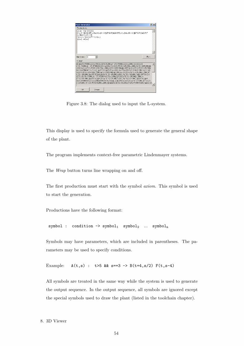
Figure 3.8: The dialog used to input the L-system.

This display is used to specify the formula used to generate the general shape

of the plant.

The program implements context-free parametric Lindenmayer systems.

The Wrap button turns line wrapping on and off.

The first production must start with the symbol axiom. This symbol is used

to start the generation.

Productions have the following format:

symbol : condition -> symbol1 symbol2 ... symboln

Symbols may have parameters, which are included in parentheses. The pa-

rameters may be used to specify conditions.

Example: A(t,s) : t>5 && s==3 -> B(t+4,s/2) F(t,s-4)

All symbols are treated in the same way while the system is used to generate

the output sequence. In the output sequence, all symbols are ignored except

the special symbols used to draw the plant (listed in the toolchain chapter).

8. 3D Viewer

54

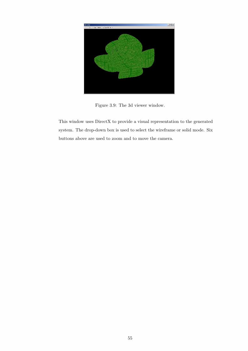
Figure 3.9: The 3d viewer window.

This window uses DirectX to provide a visual representation to the generated

system. The drop-down box is used to select the wireframe or solid mode. Six

buttons above are used to zoom and to move the camera.

55

56

Concluding Remarks

Work on this thesis led to many an interesting observation throughout the spectrum

of issues associated with the generation of plants. A large number of topics has been

covered that span over the whole plant generation toolchain. Here, thoughts arising

from these endeavours are given.

It is quite obvious that the issue central to the whole process is the question

of how to get the utmost use from the formalism of Lindenmayer systems. Sadly,

it seems adequate to conclude that the promised biologically-motivated means of

modelling organic structures in a fast and easy way has yet to come into being.

The problem with Lindenmayer systems is inherently tied to one of their main

virtues: simplicity. True, it is possible to express complex structures using only a

few productions. True, it is easy to obtain images of the same plant at different

developmental stages if the system is appropriately constructed. This does not

change the fact, however, that it is extremely difficult to extend this formalism to

cover a broad spectrum of objects. Lindenmayer systems are good at describing tree

structures, which is hardly surprising because trees are simple. As soon as more

complexity is required, they fail. One may argue that most plants do have a tree

topology and thus the added complexity is not required. The simplest example of

this limitation it the one that has been encountered while researching leaf venation:

originally, the venation pattern of the leaf was intended to be modelled using an

auxiliary Lindenmayer system. However, it proved impossible to construct a system

that would model a reasonable variety of such systems adequately as it was very

difficult to make the separate veinlets grow together. Consequently, a separate

algorithm had to be introduced. Plants may be tree like in the macro scale, but

they are certainly not so in the micro scale, nor in the scale of the whole ecosystem.

A similar argument applies to other plant features. If one wants smooth branches,

it is necessary to add a generalised cylinders to the model, which is external to

the system. If one wants flowers, another structure has to be added. This has

the effect that once we add everything that is necessary to construct a well-looking

57

plant, the whole model loses its flexibility because these addenda do not have the

developmental potential that a raw Lindenmayer system boasts: we can no longer

trace the way a plant develops. Indeed, during the development of productions, one

is fast tempted to fall into the pitfall of merely viewing the Lindenmayer system

as an exotic variation of programming in LOGO and thus lose whatever biological

founding the model might have had. Naturally, this does not mean that Lindenmayer

systems are out of place. As of now, there exists no better solution for generating

arbitrary plants.

Another aspect of plant modelling that needs to be stressed here is the huge

potential of particle systems. In the effort described in this thesis, they have been

used to model the leaf venation pattern. Their main advantage is the relatively

straightforward way of implementation, at least compared to attempts to tackle the

same issues using a more prescriptive approach. It is also easy to introduce variation

in the generated structures, because the sources are scattered randomly as well as

to model two- or even three-dimensional structures. Actually, attempts have been

made (Rodkaew et al. [2002]) to use them for modelling whole plants, but initial

results were modest at best. In the future, it will probably be possible to improve

on these results and maybe obtain a workable variation of particle systems that

works good for the modelling of the whole plant. It would also be interesting to

see how the proposal to account for stress formation in the leaf made by Couder

et al. [2002] can be used to make the particles move in a more realistic way. In this

context, it seems appropriate to note the analogy between particle and Lindenmayer

systems: if we allow the particles to have arbitrary parameters and the rules that

govern the behaviour of a particle (which may mean both modifying an attribute

of the particle or splitting it into smaller particles) to be based on an arbitrarily

defined neighbourhood of the particle (which may extend to the whole system),

then a Lindenmayer system is just a special case of a particle system constrained to

one dimension and one notion of proximity, where tokens correspond to particles. It

would be interesting to see in what practical ways the use of particle systems may

be beneficial to the modelling of plants.

In summary, it does not seem very original or innovative, but needs to be stated

that plants are inherently complex. Complex objects require complex models, which

usually require complex implementation. This thesis outlined some endeavours on

the way to a better model. It remains to be seen how fast the evolution of computer

graphics leads us to an algorithm that produces truly satisfying results.

58

Bibliography

Diogo Vieira Andrade and Luiz Henrique de Figueiredo. Empirically good approx-

imations for the relative neighbourhood graph, 2003. URL citeseer.ist.psu.

edu/vieiraandrade02empirically.html.

Jules Bloomenthal. Modeling the mighty maple. SIGGRAPH Comput. Graph.,

19(3):305–311, 1985. ISSN 0097-8930. doi: http://doi.acm.org/10.1145/325165.

325249.

Jules Bloomenthal. Skeletal Design of Natural Forms. PhD thesis, University of

Calgary, Calgary, Alta., Canada, Canada, 1995. Adviser-Brian Wyvill.

Jules Bloomenthal and Brian Wyvill. Interactive techniques for implicit modeling. In

SI3D ’90: Proceedings of the 1990 symposium on Interactive 3D graphics, pages

109–116, New York, NY, USA, 1990. ACM. ISBN 0-89791-351-5. doi: http:

//doi.acm.org/10.1145/91385.91427.

CGAL. Computational Geometry Algorithms Library. URL http://www.cgal.org.

Yves Couder, Ludovic Pauchard, Catherine Allain, Moktar Adda-Bedia, and

Stéphane Douady. The leaf venation as formed in a tensorial field. The European

Physical Journal B - Condensed Matter and Complex Systems, 28(2):135–138,

2002. ISSN 1434-6036. doi: http://doi.ieeecomputersociety.org/10.1140/epjb/

e2002-00211-1.

Pavol Federl. Modeling fracture formation on growing surfaces. PhD thesis, Uni-

versity of Calgary, Calgary, Alta., Canada, Canada, 2003. Adviser-Przemyslaw

Prusinkiewicz.

Martin Fuhrer. Hairs, textures, and shades: Improving the realism of plant models

generated with l-systems, 2005. Adviser-Przemyslaw Prusinkiewicz.

Jacob E. Goodman and Joseph O’Rourke, editors. Handbook of discrete and compu-

59

tational geometry. CRC Press, Inc., Boca Raton, FL, USA, 1997. ISBN 0-8493-

8524-5.

GPLEX. The Gardens Point Scanner Generator. URL plas.fit.qut.edu.au/

gplex/.

James Scott Hanan. Paramteric L-systems and their application to the modelling and

visualization of plants. PhD thesis, University of Regina, Regina, Saskatchewan,

Canada, 1992. Adviser-Przemyslaw Prusinkiewicz.

J. Hart and B. Baker. Implicit modeling of tree surfaces, 1996. URL citeseer.

ist.psu.edu/hart96implicit.html.

ImageMagick. The ImageMagick Software Suite. URL www.imagemagick.org.

Lars Mundermann, Peter MacMurchy, Juraj Pivovarov, and Przemyslaw

Prusinkiewicz. Modeling lobed leaves. cgi, 00:60, 2003. ISSN 1530-1052. doi:

http://doi.ieeecomputersociety.org/10.1109/CGI.2003.1214448.

Peter E. Oppenheimer. Real time design and animation of fractal plants and trees.

SIGGRAPH Comput. Graph., 20(4):55–64, 1986. ISSN 0097-8930. doi: http:

//doi.acm.org/10.1145/15886.15892.

Przemyslaw Prusinkiewicz and Aristid Lindenmayer. The algorithmic beauty of

plants. Springer-Verlag New York, Inc., New York, NY, USA, 1996. ISBN 0-

387-94676-4.

Przemyslaw Prusinkiewicz, Lars Mündermann, Radoslaw Karwowski, and Brendan

Lane. The use of positional information in the modeling of plants. In SIGGRAPH

’01: Proceedings of the 28th annual conference on Computer graphics and in-

teractive techniques, pages 289–300, New York, NY, USA, 2001. ACM. ISBN

1-58113-374-X. doi: http://doi.acm.org/10.1145/383259.383291.

Yodthong Rodkaew, Prabhas Chongstitvatana, Suchida Siripant, and Chidchanok

Lursinsap. Modeling and visualization of leaf venation patterns. In International

Conference on Computational Mathematics and Modeling, 2002.

Adam Runions, Martin Fuhrer, Brendan Lane, Pavol Federl, Anne-Gaëlle Rolland-

Lagan, and Przemyslaw Prusinkiewicz. Modeling and visualization of leaf venation

patterns. In SIGGRAPH ’05: ACM SIGGRAPH 2005 Papers, pages 702–711,

New York, NY, USA, 2005. ACM. doi: http://doi.acm.org/10.1145/1186822.

1073251.

60

Arto Salomaa. Formal languages. Academic Press, New York and London, 1973.

ISBN 0126157505.

David Salomon. Computer Graphics and Geometric Modeling. Springer-Verlag New

York, Inc., Secaucus, NJ, USA, 1999. ISBN 0387986820.

John M. Snyder and James T. Kajiya. Generative modeling: a symbolic system for

geometric modeling. SIGGRAPH Comput. Graph., 26(2):369–378, 1992. ISSN

0097-8930. doi: http://doi.acm.org/10.1145/142920.134094.

Julis Taulor-Hell and Gladimir Baranoski. State of the art in the realistic simula-

tion of plant leaf venation systems. Technical Report CS-2002-17, University of

Waterloo, Departament of Computer Science, Waterloo, Ontario, April 2002.

G. Toussaint. The relative neighbourhood graph of a finite planar set, 1980. URL

citeseer.ist.psu.edu/toussaint80relative.html.

Xi Wang, Lifeng Wang, Ligang Liu, Shimin Hu, and Baining Guo. Interactive

modeling of tree bark. In PG ’03: Proceedings of the 11th Pacific Conference

on Computer Graphics and Applications, page 83, Washington, DC, USA, 2003.

IEEE Computer Society. ISBN 0-7695-2028-6.

Wikipedia. Wikipedia, the free encyclopedia. URL wikipedia.org.

61

Warszawa, dnia 11. 03. 2008 r.

Oświadczenie

Oświadczam, że pracę inżynierską pod tytułem: ”Generating 3D Plants” (”Gene-

rowanie trójwymiarowych modeli roślin”), której promotorem jest Dr. Paweł Ko-

towski wykonałem samodzielnie, co poświadczam własnoręcznym podpisem.

.............................................