
Data Warehouse Physical Design: Part II
44
Robert Wrembel Poznan University of Technology Institute of Computing Science [email protected] www.cs.put.poznan.pl/rwrembel Data Warehouse Physical Design: Part II © Robert Wrembel (Poznan University of Technology, Poland) Lecture outline Row storage vs. Column storage Data compression Materialization Small summary data Materialized views and query rewriting Partitioning MOLAP 2
Transcript of Data Warehouse Physical Design: Part II
Robert Wrembel
Poznan University of Technology
Institute of Computing Science
www.cs.put.poznan.pl/rwrembel
Data Warehouse Physical Design:
Part II
© Robert Wrembel (Poznan University of Technology, Poland)
Lecture outline
Row storage vs. Column storage
Data compression
Materialization
Small summary data
Materialized views and query rewriting
Partitioning
MOLAP
2
© Robert Wrembel (Poznan University of Technology, Poland)
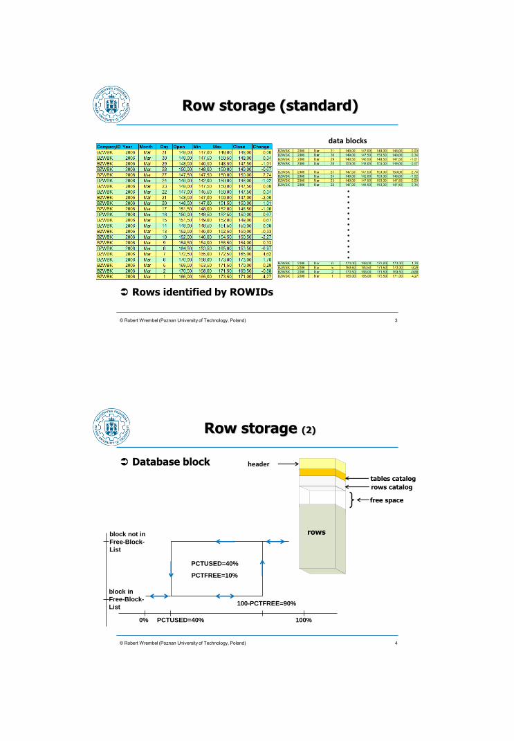
Row storage (standard)
data blocks
Rows identified by ROWIDs
. . . . . . . . . . . . .
3
Row storage (2)
Database block
© Robert Wrembel (Poznan University of Technology, Poland)
rows
free space
header
tables catalog
rows catalog
PCTUSED=40% 0% 100%
100-PCTFREE=90%
PCTUSED=40%
PCTFREE=10%
block in
Free-Block-
List
block not in
Free-Block-
List
4
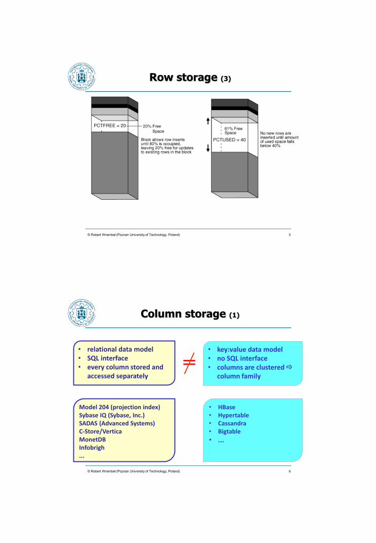
Row storage (3)
© Robert Wrembel (Poznan University of Technology, Poland) 5
Column storage (1)
© Robert Wrembel (Poznan University of Technology, Poland)
• key:value data model • no SQL interface • columns are clustered
column family
• relational data model • SQL interface • every column stored and
accessed separately =
• HBase • Hypertable • Cassandra • Bigtable
• ...
Model 204 (projection index) Sybase IQ (Sybase, Inc.) SADAS (Advanced Systems) C-Store/Vertica MonetDB Infobrigh ...
6

© Robert Wrembel (Poznan University of Technology, Poland)
Column storage (2)
Rows identified by slot numbers (in a block)
data blocks
slot 1
7
Column storage (3)
Database block
no free space
better space utilization
© Robert Wrembel (Poznan University of Technology, Poland)
rows
header
8

SQL Server
Ver. 2012 and higher
Divide rows into row groups of about one million rows each
Compress each row group independently - dictionary compression for string columns
Store each column segment as a separate BLOB P.-A. Larson, E. N. Hanson, S. L. Price: Columnar Storage in SQL Server
2012. IEEE Data Eng. Bull. 35(1), 2012
© Robert Wrembel (Poznan University of Technology, Poland) 9
Query processing example
© Robert Wrembel (Poznan University of Technology, Poland)
select Open
from StockQuotes
where CompanyID='BZWBK'
and Year=2006
and Month='Mar'
and Day=8; list of positions (slot numbers) of values fulfilling the predicate represented as: • array or • bit vector or • set of position ranges
One table query
10
© Robert Wrembel (Poznan University of Technology, Poland)
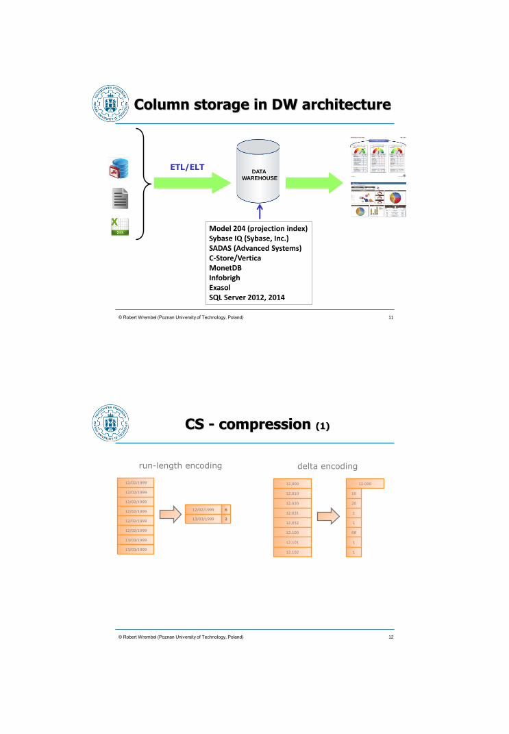
Column storage in DW architecture
DATA
WAREHOUSE
ETL/ELT
11
Model 204 (projection index) Sybase IQ (Sybase, Inc.) SADAS (Advanced Systems) C-Store/Vertica MonetDB Infobrigh Exasol SQL Server 2012, 2014
© Robert Wrembel (Poznan University of Technology, Poland)
CS - compression (1)
12.000
12.010
12.030
12.031
12.032
12.100
12.101
12.102
delta encoding
12.000
10
20
1
1
68
1
1
12/02/1999
12/02/1999
12/02/1999
12/02/1999
12/02/1999
12/02/1999
13/03/1999
13/03/1999
12/02/1999 6
run-length encoding
13/03/1999 2
12

© Robert Wrembel (Poznan University of Technology, Poland)
CS - compression (2)
mapping table
Discrete domain encoding
13
© Robert Wrembel (Poznan University of Technology, Poland)
RS - compression (1)
Oracle
Dictionary compression (DB2)
Like discrete domain encoding
dictionary stored in
• a dedicated table
• data block header
14
© Robert Wrembel (Poznan University of Technology, Poland)
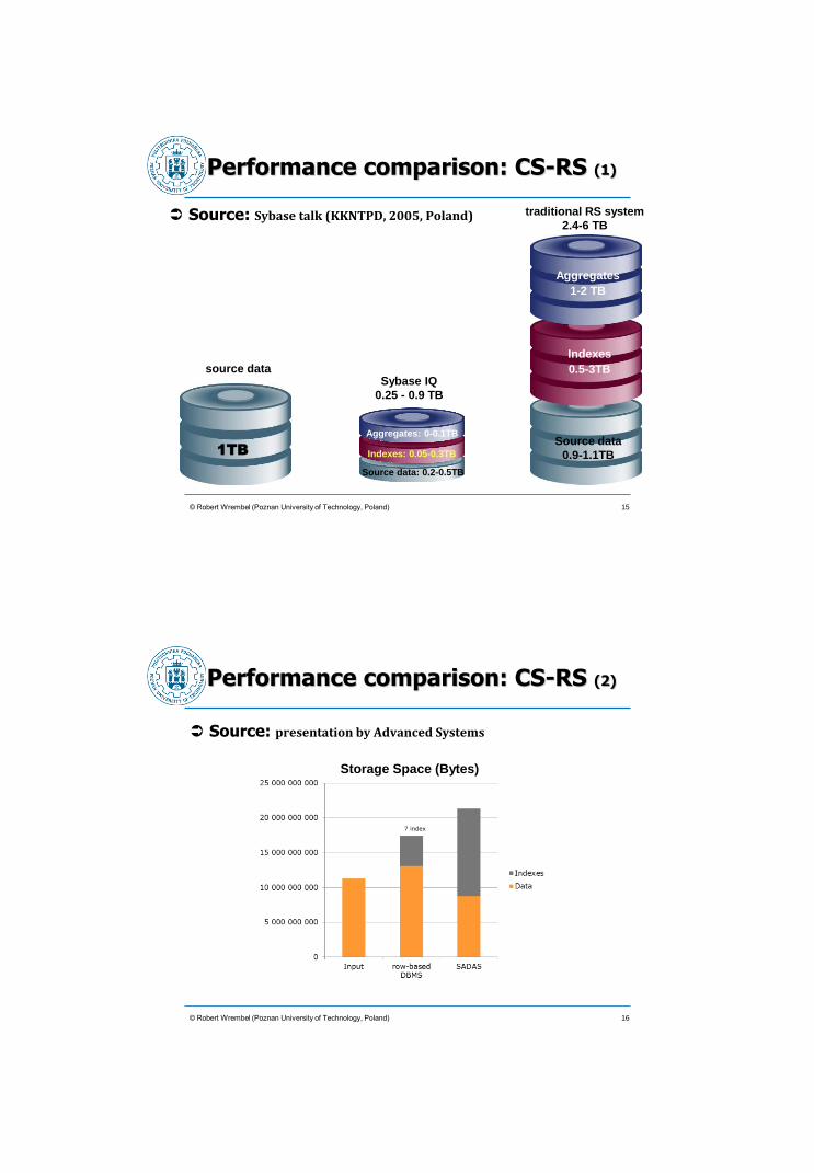
Performance comparison: CS-RS (1)
Source: Sybase talk (KKNTPD, 2005, Poland)
1TB
Source data: 0.2-0.5TB
Indexes: 0.05-0.3TB
Aggregates: 0-0.1TB
Aggregates
1-2 TB
Indexes
0.5-3TB
Source data
0.9-1.1TB
traditional RS system
2.4-6 TB
Sybase IQ
0.25 - 0.9 TB
source data
15
© Robert Wrembel (Poznan University of Technology, Poland)
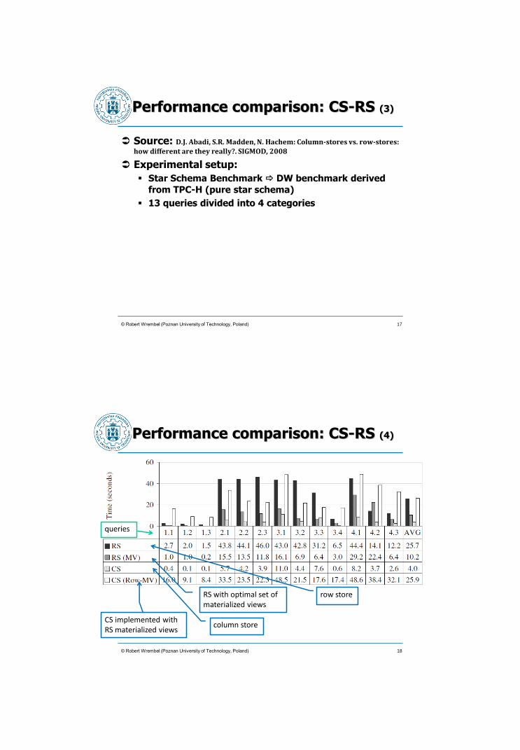
Performance comparison: CS-RS (2)
Source: presentation by Advanced Systems
Storage Space (Bytes)
7 index
16
Performance comparison: CS-RS (3)
Source: D.J. Abadi, S.R. Madden, N. Hachem: Column-stores vs. row-stores:
how different are they really?. SIGMOD, 2008
Experimental setup:
Star Schema Benchmark DW benchmark derived
from TPC-H (pure star schema)
13 queries divided into 4 categories
© Robert Wrembel (Poznan University of Technology, Poland) 17
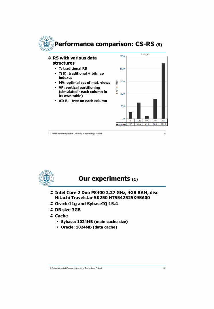
Performance comparison: CS-RS (4)
© Robert Wrembel (Poznan University of Technology, Poland)
row store RS with optimal set of materialized views
column store CS implemented with RS materialized views
queries
18
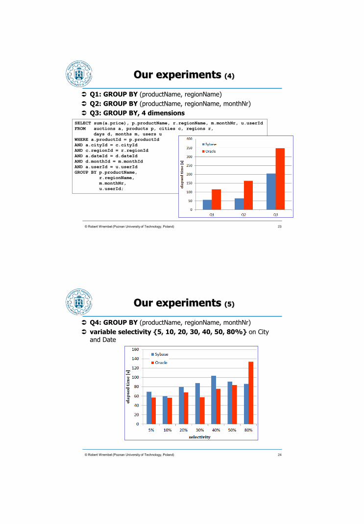
Performance comparison: CS-RS (5)
RS with various data structures
T: traditional RS
T(B): traditional + bitmap indexes
MV: optimal set of mat. views
VP: vertical partitioning (simulated - each column in its own table)
AI: B+-tree on each column
© Robert Wrembel (Poznan University of Technology, Poland) 19
Our experiments (1)
Intel Core 2 Duo P8400 2,27 GHz, 4GB RAM, disc Hitachi Travelstar 5K250 HTS542525K9SA00
Oracle11g and SybaseIQ 15.4
DB size 3GB
Cache
Sybase: 1024MB (main cache size)
Oracle: 1024MB (data cache)
© Robert Wrembel (Poznan University of Technology, Poland) 20

Our experiments (2)
Indexes
SybaseIQ
• Fast Projection (default) on all columns for
projection optimization
• High Group (default) on UNIQUE, PRIMARY
KEY, FOREIGN KEY
Oracle
• PRIMARY KEY (default)
• FOREIGN KEY
© Robert Wrembel (Poznan University of Technology, Poland) 21
Our experiments (3)
© Robert Wrembel (Poznan University of Technology, Poland) 22
Our experiments (4)
Q1: GROUP BY (productName, regionName)
Q2: GROUP BY (productName, regionName, monthNr)
Q3: GROUP BY, 4 dimensions
© Robert Wrembel (Poznan University of Technology, Poland)
SELECT sum(a.price), p.productName, r.regionName, m.monthNr, u.userId
FROM auctions a, products p, cities c, regions r,
days d, months m, users u
WHERE a.productId = p.productId
AND a.cityId = c.cityId
AND c.regionId = r.regionId
AND a.dateId = d.dateId
AND d.monthId = m.monthId
AND a.userId = u.userId
GROUP BY p.productName,
r.regionName,
m.monthNr,
u.userId;
23
Our experiments (5)
© Robert Wrembel (Poznan University of Technology, Poland)
Q4: GROUP BY (productName, regionName, monthNr)
variable selectivity {5, 10, 20, 30, 40, 50, 80%} on City and Date
24

© Robert Wrembel (Poznan University of Technology, Poland)
Our experiments (6)
Q5: GROUP BY ROLLUP (productName, regionName)
Q6: GROUP BY ROLLUP (productName, countryName, monthNr)
25
Our experiments (7)
Q7: one table query
© Robert Wrembel (Poznan University of Technology, Poland)
SELECT sum(a.price), a.productId, a.cityId, a.dateId
FROM Auctions a
GROUP BY productId, cityId, dateId;
26

© Robert Wrembel (Poznan University of Technology, Poland)
Materialization - SMA
SMA - Small Materialized Aggregates (G. Moerkotte, VLDB, 1998)
disk data are divided into buckets
every bucket has associated SMA
SMA bucket1 TimeKey max: 31.03.2006 TimeKey min: 27.03.2006 count: 5
SMA bucket2 TimeKey max: 24.03.2006 TimeKey min: 20.03.2006 count: 5
SMA bucket3 TimeKey max: 17.03.2006 TimeKey min: 13.03.2006 count: 5
27
SMA
SMA
defined on an ordering attribute
used for filtering buckets
e.g. select ... from ... where TimeKey > '22-Mar-2006'
© Robert Wrembel (Poznan University of Technology, Poland)
SMA bucket1 TimeKey max: 31.03.2006 TimeKey min: 27.03.2006 count: 5
SMA bucket2 TimeKey max: 24.03.2006 TimeKey min: 20.03.2006 count: 5
SMA bucket3 TimeKey max: 17.03.2006 TimeKey min: 13.03.2006 count: 5
28
© Robert Wrembel (Poznan University of Technology, Poland)
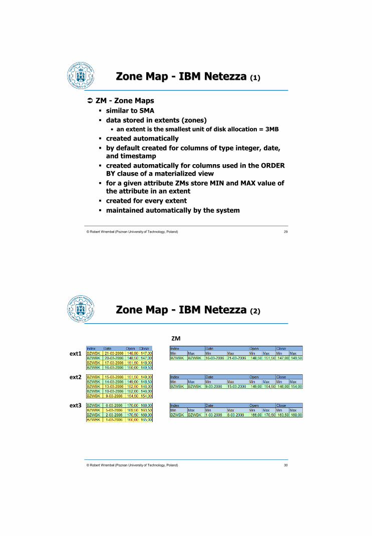
Zone Map - IBM Netezza (1)
ZM - Zone Maps
similar to SMA
data stored in extents (zones)
• an extent is the smallest unit of disk allocation = 3MB
created automatically
by default created for columns of type integer, date, and timestamp
created automatically for columns used in the ORDER BY clause of a materialized view
for a given attribute ZMs store MIN and MAX value of the attribute in an extent
created for every extent
maintained automatically by the system
29
Zone Map - IBM Netezza (2)
© Robert Wrembel (Poznan University of Technology, Poland)
ext1
ext2
ext3
ZM
30
© Robert Wrembel (Poznan University of Technology, Poland)
Zone Filters (1)
Zone filters, Bit vector filters, Zone indexes (G. Graefe, DAWAK, 2009)
ZF - Zone Filter similar to SMA and ZM
ZF maintained for each zone and attribute
ZF stores m consecutive MIN and MAX values
• if m=1 then ZF equivalent to ZM
• if m=1 then either MIN or MAX can be NULL not
useful for filtering zones
• if m=2 then in the presence of NULLs the second value of MIN or MAX is NOT NULL
31
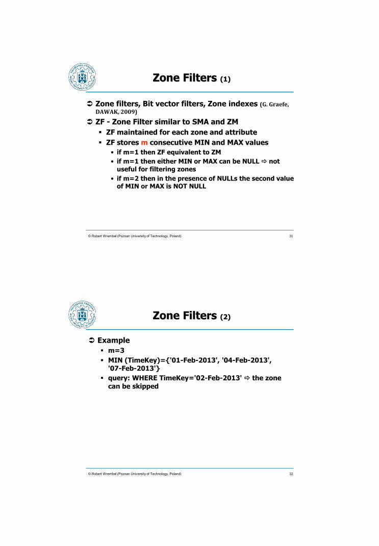
Zone Filters (2)
Example
m=3
MIN (TimeKey)={'01-Feb-2013', '04-Feb-2013', '07-Feb-2013'}
query: WHERE TimeKey='02-Feb-2013' the zone
can be skipped
© Robert Wrembel (Poznan University of Technology, Poland) 32
Zone Filters (3)
BVF - Bit Vector Filter
maintained for each zone and for each column
provides a synopsis of the actual values
ZI - Zone Index
supports searching within a zone
a dedicated ZI maintained for a zone
© Robert Wrembel (Poznan University of Technology, Poland) 33
© Robert Wrembel (Poznan University of Technology, Poland)
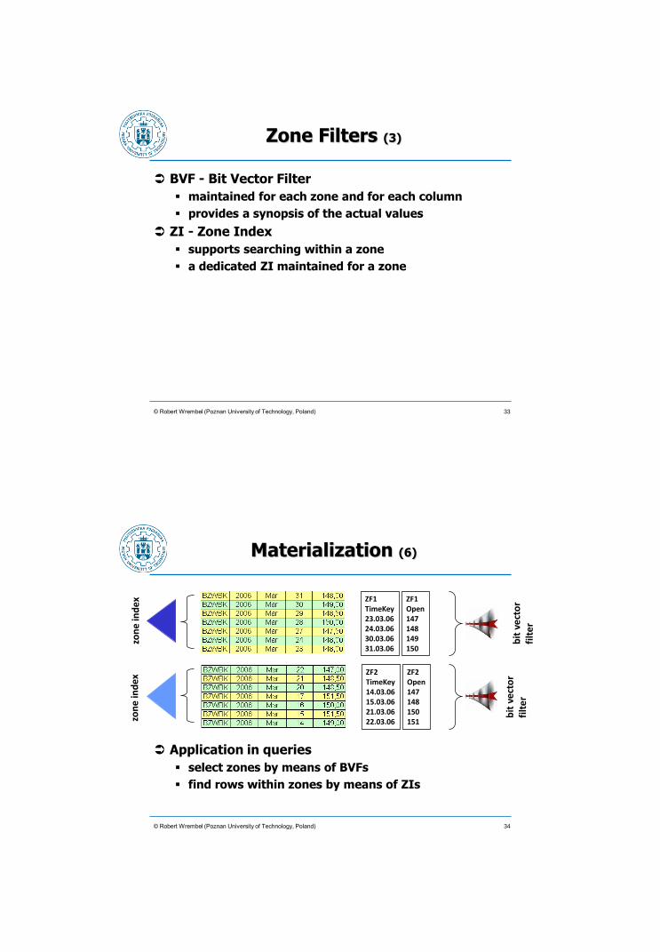
Materialization (6)
Application in queries
select zones by means of BVFs
find rows within zones by means of ZIs
ZF1 TimeKey 23.03.06 24.03.06 30.03.06 31.03.06
ZF1 Open 147 148 149 150
ZF2 TimeKey 14.03.06 15.03.06 21.03.06 22.03.06
ZF2 Open 147 148 150 151
zon
e in
dex
zo
ne
ind
ex
bit
ve
cto
r fi
lte
r
bit
ve
cto
r fi
lte
r
34
Materialized query
The result of a query persistently stored in a database
table (naive approach)
materialized view (Oracle, IBM Netezza), materialized query table/ summary table (DB2), indexed view (SQL Server)
• additional functionality
– refreshing
– query rewriting
© Robert Wrembel (Poznan University of Technology, Poland) 35
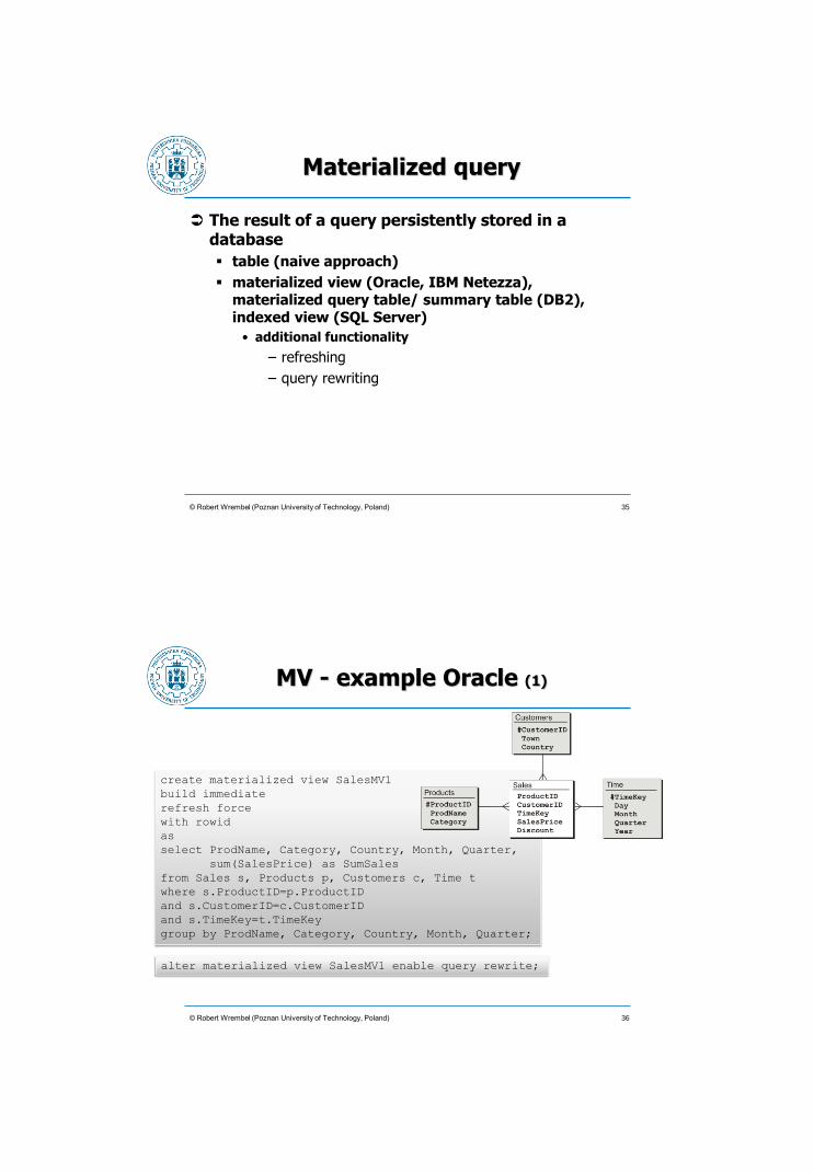
MV - example Oracle (1)
© Robert Wrembel (Poznan University of Technology, Poland)
create materialized view SalesMV1
build immediate
refresh force
with rowid
as
select ProdName, Category, Country, Month, Quarter,
sum(SalesPrice) as SumSales
from Sales s, Products p, Customers c, Time t
where s.ProductID=p.ProductID
and s.CustomerID=c.CustomerID
and s.TimeKey=t.TimeKey
group by ProdName, Category, Country, Month, Quarter;
alter materialized view SalesMV1 enable query rewrite;
36
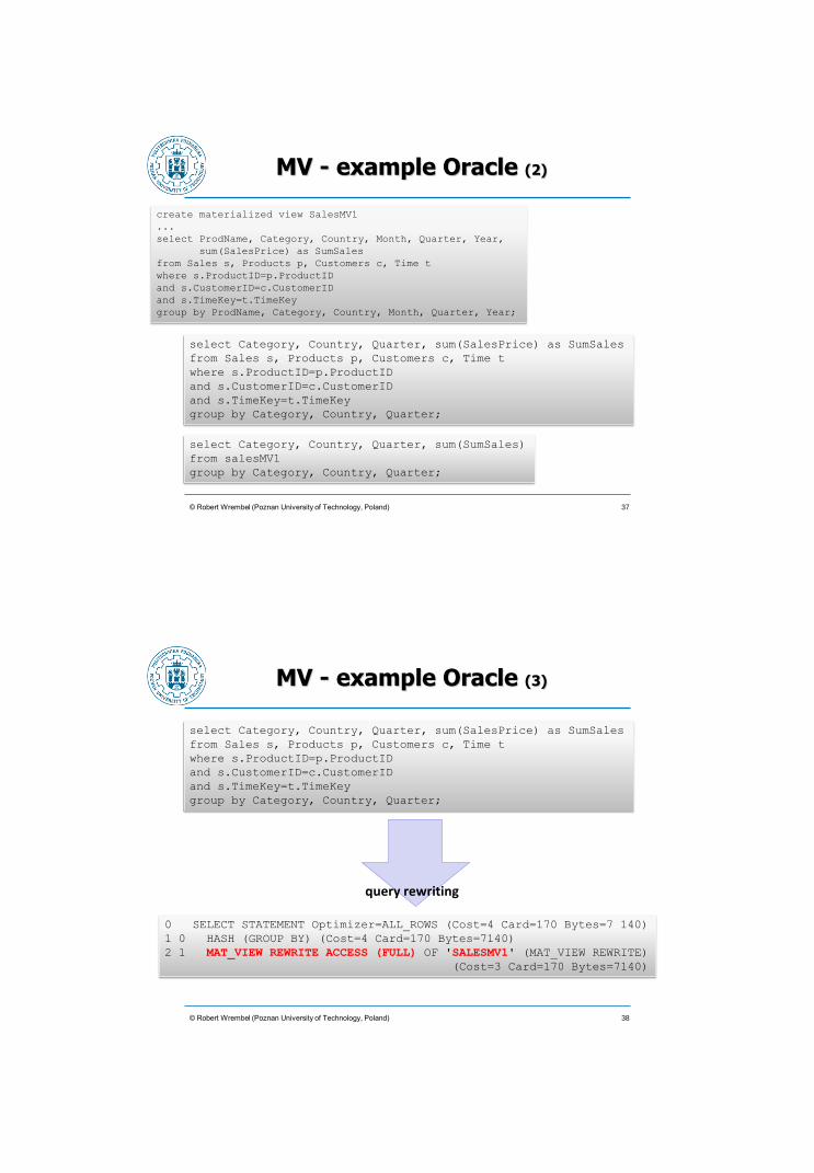
MV - example Oracle (2)
© Robert Wrembel (Poznan University of Technology, Poland)
select Category, Country, Quarter, sum(SalesPrice) as SumSales
from Sales s, Products p, Customers c, Time t
where s.ProductID=p.ProductID
and s.CustomerID=c.CustomerID
and s.TimeKey=t.TimeKey
group by Category, Country, Quarter;
select Category, Country, Quarter, sum(SumSales)
from salesMV1
group by Category, Country, Quarter;
create materialized view SalesMV1
...
select ProdName, Category, Country, Month, Quarter, Year,
sum(SalesPrice) as SumSales
from Sales s, Products p, Customers c, Time t
where s.ProductID=p.ProductID
and s.CustomerID=c.CustomerID
and s.TimeKey=t.TimeKey
group by ProdName, Category, Country, Month, Quarter, Year;
37
MV - example Oracle (3)
© Robert Wrembel (Poznan University of Technology, Poland)
select Category, Country, Quarter, sum(SalesPrice) as SumSales
from Sales s, Products p, Customers c, Time t
where s.ProductID=p.ProductID
and s.CustomerID=c.CustomerID
and s.TimeKey=t.TimeKey
group by Category, Country, Quarter;
0 SELECT STATEMENT Optimizer=ALL_ROWS (Cost=4 Card=170 Bytes=7 140)
1 0 HASH (GROUP BY) (Cost=4 Card=170 Bytes=7140)
2 1 MAT_VIEW REWRITE ACCESS (FULL) OF 'SALESMV1' (MAT_VIEW REWRITE)
(Cost=3 Card=170 Bytes=7140)
query rewriting
38
© Robert Wrembel (Poznan University of Technology, Poland)
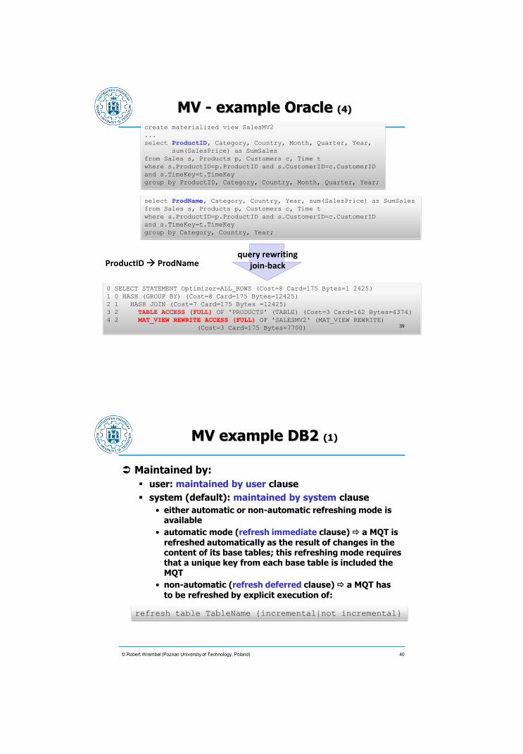
MV - example Oracle (4)
39 R.Wrembel - Poznan University of Technology
create materialized view SalesMV2
...
select ProductID, Category, Country, Month, Quarter, Year,
sum(SalesPrice) as SumSales
from Sales s, Products p, Customers c, Time t
where s.ProductID=p.ProductID and s.CustomerID=c.CustomerID
and s.TimeKey=t.TimeKey
group by ProductID, Category, Country, Month, Quarter, Year;
0 SELECT STATEMENT Optimizer=ALL_ROWS (Cost=8 Card=175 Bytes=1 2425)
1 0 HASH (GROUP BY) (Cost=8 Card=175 Bytes=12425)
2 1 HASH JOIN (Cost=7 Card=175 Bytes =12425)
3 2 TABLE ACCESS (FULL) OF 'PRODUCTS' (TABLE) (Cost=3 Card=162 Bytes=4374)
4 2 MAT_VIEW REWRITE ACCESS (FULL) OF 'SALESMV2' (MAT_VIEW REWRITE)
(Cost=3 Card=175 Bytes=7700)
query rewriting join-back
select ProdName, Category, Country, Year, sum(SalesPrice) as SumSales
from Sales s, Products p, Customers c, Time t
where s.ProductID=p.ProductID and s.CustomerID=c.CustomerID
and s.TimeKey=t.TimeKey
group by Category, Country, Year;
ProductID ProdName
39
MV example DB2 (1)
Maintained by:
user: maintained by user clause
system (default): maintained by system clause
• either automatic or non-automatic refreshing mode is available
• automatic mode (refresh immediate clause) a MQT is
refreshed automatically as the result of changes in the content of its base tables; this refreshing mode requires that a unique key from each base table is included the MQT
• non-automatic (refresh deferred clause) a MQT has
to be refreshed by explicit execution of:
© Robert Wrembel (Poznan University of Technology, Poland)
refresh table TableName {incremental|not incremental}
40
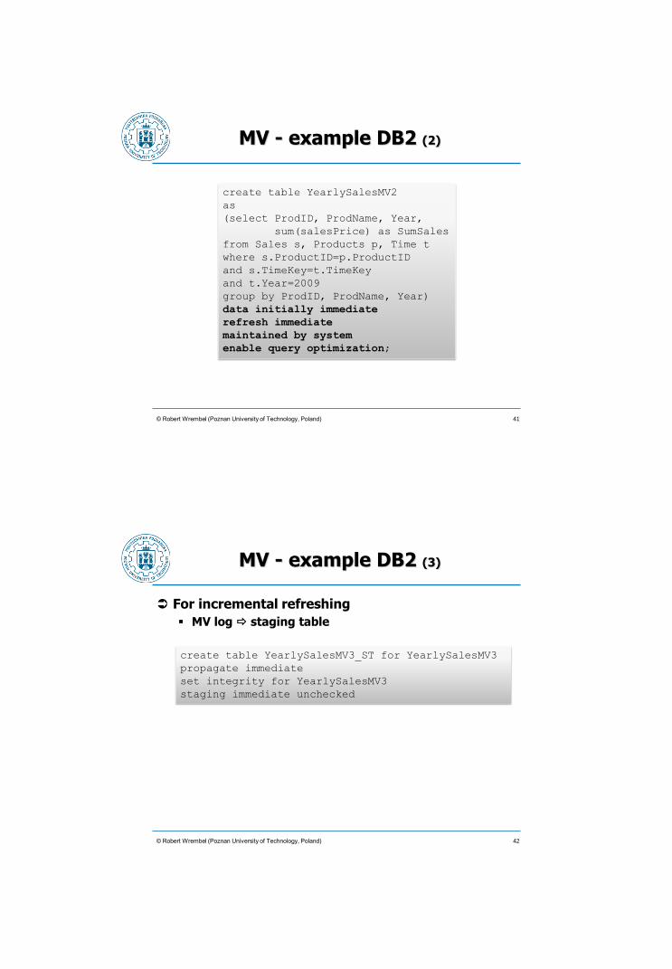
MV - example DB2 (2)
© Robert Wrembel (Poznan University of Technology, Poland)
create table YearlySalesMV2
as
(select ProdID, ProdName, Year,
sum(salesPrice) as SumSales
from Sales s, Products p, Time t
where s.ProductID=p.ProductID
and s.TimeKey=t.TimeKey
and t.Year=2009
group by ProdID, ProdName, Year)
data initially immediate
refresh immediate
maintained by system
enable query optimization;
41
MV - example DB2 (3)
For incremental refreshing
MV log staging table
© Robert Wrembel (Poznan University of Technology, Poland)
create table YearlySalesMV3_ST for YearlySalesMV3
propagate immediate
set integrity for YearlySalesMV3
staging immediate unchecked
42
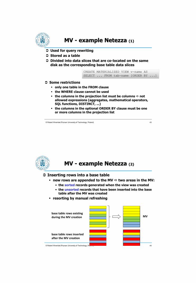
MV - example Netezza (1)
Used for query rewriting
Stored as a table
Divided into data slices that are co-located on the same disk as the corresponding base table data slices
© Robert Wrembel (Poznan University of Technology, Poland)
CREATE MATERIALIZED VIEW v-name AS
SELECT ... FROM tab-name [ORDER BY ...]
Some restrictions
only one table in the FROM clause
the WHERE clause cannot be used
the columns in the projection list must be columns not
allowed expressions (aggregates, mathematical operators, SQL functions, DISTINCT, ...)
the columns in the optional ORDER BY clause must be one or more columns in the projection list
43
MV - example Netezza (2)
Inserting rows into a base table
new rows are appended to the MV two areas in the MV:
• the sorted records generated when the view was created
• the unsorted records that have been inserted into the base table after the MV was created
resorting by manual refreshing
© Robert Wrembel (Poznan University of Technology, Poland)
base table rows existing during the MV creation MV
base table rows inserted after the MV creation
44

MV - example Netezza (3)
Suspending MV making it inactive
Refreshing MV
manually the REFRESH option
automatically setting a refresh threshold
• the threshold specifies the percentage of unsorted data in the materialized view, value from 1 to 99 (default 20)
• the thresholds allows to refresh all the materialized views associated with a base table
© Robert Wrembel (Poznan University of Technology, Poland)
ALTER VIEW MV-name MATERIALIZE {REFRESH | SUSPEND}
The system creates zone maps for all columns in a MV that have data types integer, date, or timestamp
45
MV example - SQL Server
MV is created by creating a unique clustered index on a view (clustering data by the value of the indexed column)
The index causes that the view is materialized
© Robert Wrembel (Poznan University of Technology, Poland)
create view YearlySalesMV
with schemabinding
as
select ProdID, ProdName, Year, sum(salesPrice) as SumSales
from Sales s, Products p, Time t
where s.ProductID=p.ProductID
and s.TimeKey=t.TimeKey
and t.Year=2009
group by ProdID, ProdName, Year
create unique clustered index Indx_ProdID
on YearlySalesMV(ProdID, ProdName, Year)
prevents from modifying base tables' schemas as long as the view exists
46
MV - SQL Server
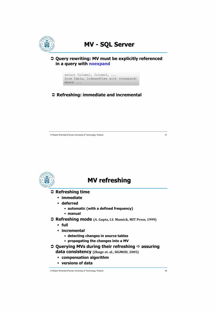
Query rewriting: MV must be explicitly referenced in a query with noexpand
© Robert Wrembel (Poznan University of Technology, Poland)
select Column1, Column2, ...
from Table, IndexedView with (noexpand)
where ...
Refreshing: immediate and incremental
47
MV refreshing
Refreshing time
immediate
deferred
• automatic (with a defined frequency)
• manual
Refreshing mode (A. Gupta, I.S. Mumick, MIT Press, 1999)
full
incremental
• detecting changes in source tables
• propagating the changes into a MV
Querying MVs during their refreshing assuring
data consistency (Zhuge et. al., SIGMOD, 2005)
compensation algorithm
versions of data
© Robert Wrembel (Poznan University of Technology, Poland) 48
MV design
Designing the optimal set of MVs
Typically for a given query workload
Constraints
minimizing response time for the largest number of queries
minimizing response time for the most expensive queries
minimizing costs of refreshing MVs
minimizing disk space
Physical design advisors
© Robert Wrembel (Poznan University of Technology, Poland) 49
© Robert Wrembel (Poznan University of Technology, Poland)
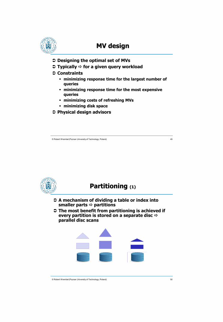
Partitioning (1)
A mechanism of dividing a table or index into smaller parts partitions
The most benefit from partitioning is achieved if every partition is stored on a separate disc parallel disc scans
50
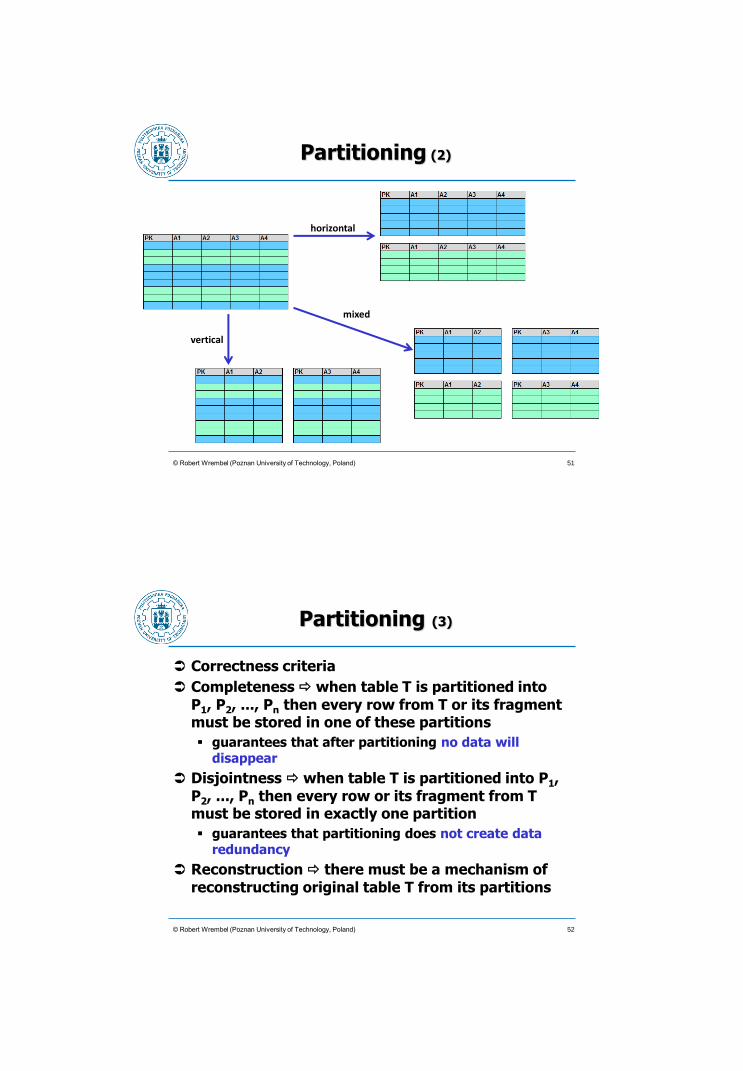
Partitioning (2)
© Robert Wrembel (Poznan University of Technology, Poland)
horizontal
vertical
mixed
51
Partitioning (3)
Correctness criteria
Completeness when table T is partitioned into P1, P2, ..., Pn then every row from T or its fragment must be stored in one of these partitions
guarantees that after partitioning no data will disappear
Disjointness when table T is partitioned into P1,
P2, ..., Pn then every row or its fragment from T must be stored in exactly one partition
guarantees that partitioning does not create data redundancy
Reconstruction there must be a mechanism of
reconstructing original table T from its partitions
© Robert Wrembel (Poznan University of Technology, Poland) 52

Partitioning (4)
In horizontal partitioning rows are divided into subsets based on the value of partitioning attribute(s)
Horizontal partitioning techniques
hash
range-based
set-based
round-robin
© Robert Wrembel (Poznan University of Technology, Poland) 53
Example Oracle (1)
Range partitioning
© Robert Wrembel (Poznan University of Technology, Poland)
create table Sales_Range_TKey
(ProductID varchar2(8) not null references Products(ProductID),
TimeKey date not null references time(TimeKey),
CustomerID varchar2(10) not null references Customers(CustomerID),
SalesPrice number(6,2))
PARTITION by RANGE (TimeKey)
(partition Sales_1Q_2009
values less than (TO_DATE(’01-04-2009’, ’DD-MM-YYYY’))
tablespace Data01,
partition Sales_2Q_2009
values less than (TO_DATE(’01-07-2009’, ’DD-MM-YYYY’))
tablespace Data02,
partition Sales_3Q_2009
values less than (TO_DATE(’01-10-2009’, ’DD-MM-YYYY’))
tablespace Data03,
partition Sales_4Q_2009
values less than (TO_DATE(’01-01-2010’, ’DD-MM-YYYY’))
tablespace Data04,
partition Sales_Others
values less than (MAXVALUE) tablespace Data05); 54
© Robert Wrembel (Poznan University of Technology, Poland)
Example Oracle (2)
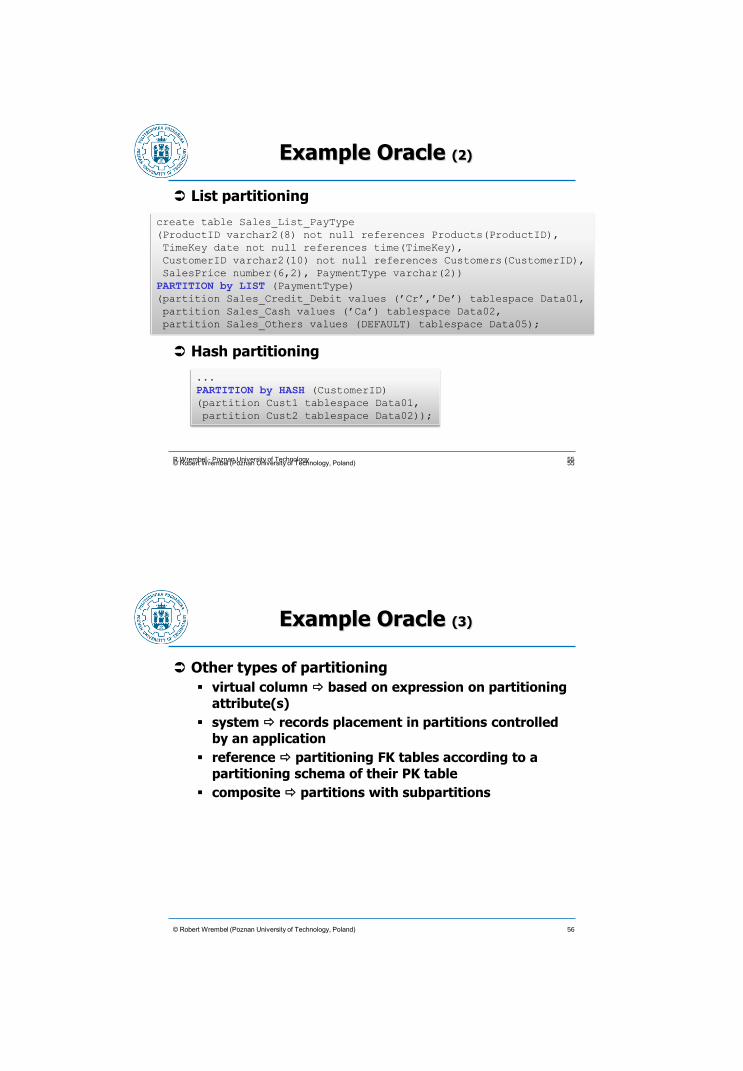
List partitioning
55 R.Wrembel - Poznan University of Technology
create table Sales_List_PayType
(ProductID varchar2(8) not null references Products(ProductID),
TimeKey date not null references time(TimeKey),
CustomerID varchar2(10) not null references Customers(CustomerID),
SalesPrice number(6,2), PaymentType varchar(2))
PARTITION by LIST (PaymentType)
(partition Sales_Credit_Debit values (’Cr’,’De’) tablespace Data01,
partition Sales_Cash values (’Ca’) tablespace Data02,
partition Sales_Others values (DEFAULT) tablespace Data05);
Hash partitioning
...
PARTITION by HASH (CustomerID)
(partition Cust1 tablespace Data01,
partition Cust2 tablespace Data02));
55
Example Oracle (3)
Other types of partitioning
virtual column based on expression on partitioning
attribute(s)
system records placement in partitions controlled
by an application
reference partitioning FK tables according to a
partitioning schema of their PK table
composite partitions with subpartitions
© Robert Wrembel (Poznan University of Technology, Poland) 56
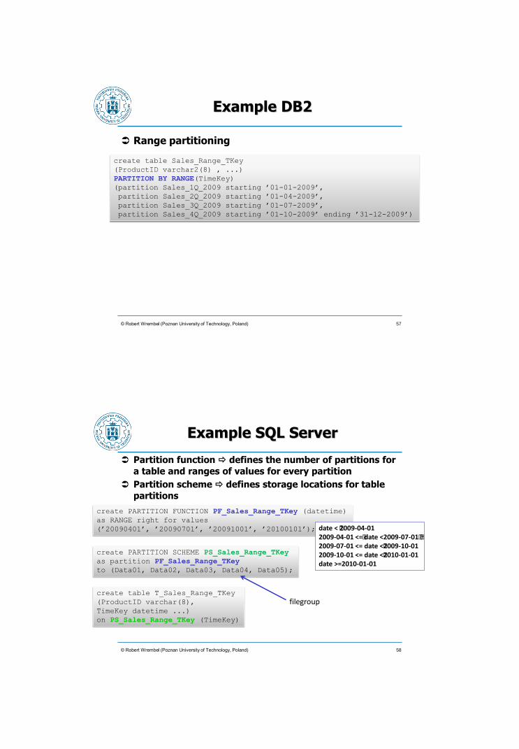
Example DB2
Range partitioning
© Robert Wrembel (Poznan University of Technology, Poland)
create table Sales_Range_TKey
(ProductID varchar2(8) , ...)
PARTITION BY RANGE(TimeKey)
(partition Sales_1Q_2009 starting ’01-01-2009’,
partition Sales_2Q_2009 starting ’01-04-2009’,
partition Sales_3Q_2009 starting ’01-07-2009’,
partition Sales_4Q_2009 starting ’01-10-2009’ ending ’31-12-2009’)
57
Example SQL Server
Partition function defines the number of partitions for
a table and ranges of values for every partition
Partition scheme defines storage locations for table
partitions
© Robert Wrembel (Poznan University of Technology, Poland)
create PARTITION FUNCTION PF_Sales_Range_TKey (datetime)
as RANGE right for values
(’20090401’, ’20090701’, ’20091001’, ’20100101’); date < �2009-04-01 2009-04-01 <=� date <2009-07-01� � 2009-07-01 <= date <�2009-10-01 2009-10-01 <= date <�2010-01-01 date >=2010-01-01
create PARTITION SCHEME PS_Sales_Range_TKey
as partition PF_Sales_Range_TKey
to (Data01, Data02, Data03, Data04, Data05);
create table T_Sales_Range_TKey
(ProductID varchar(8),
TimeKey datetime ...)
on PS_Sales_Range_TKey (TimeKey)
filegroup
58
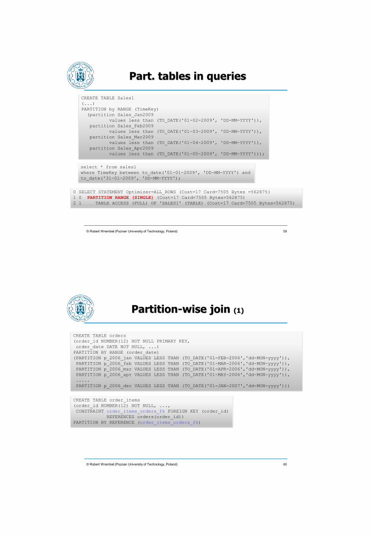
Part. tables in queries
© Robert Wrembel (Poznan University of Technology, Poland)
CREATE TABLE Sales1
(...)
PARTITION by RANGE (TimeKey)
(partition Sales_Jan2009
values less than (TO_DATE('01-02-2009', 'DD-MM-YYYY')),
partition Sales_Feb2009
values less than (TO_DATE('01-03-2009', 'DD-MM-YYYY')),
partition Sales_Mar2009
values less than (TO_DATE('01-04-2009', 'DD-MM-YYYY')),
partition Sales_Apr2009
values less than (TO_DATE('01-05-2009', 'DD-MM-YYYY')));
select * from sales1
where TimeKey between to_date('01-01-2009', 'DD-MM-YYYY') and
to_date('31-01-2009', 'DD-MM-YYYY');
0 SELECT STATEMENT Optimizer=ALL_ROWS (Cost=17 Card=7505 Bytes =562875)
1 0 PARTITION RANGE (SINGLE) (Cost=17 Card=7505 Bytes=562875)
2 1 TABLE ACCESS (FULL) OF 'SALES1' (TABLE) (Cost=17 Card=7505 Bytes=562875)
59
Partition-wise join (1)
© Robert Wrembel (Poznan University of Technology, Poland)
CREATE TABLE orders
(order_id NUMBER(12) NOT NULL PRIMARY KEY,
order_date DATE NOT NULL, ...)
PARTITION BY RANGE (order_date)
(PARTITION p_2006_jan VALUES LESS THAN (TO_DATE('01-FEB-2006','dd-MON-yyyy')),
PARTITION p_2006_feb VALUES LESS THAN (TO_DATE('01-MAR-2006','dd-MON-yyyy')),
PARTITION p_2006_mar VALUES LESS THAN (TO_DATE('01-APR-2006','dd-MON-yyyy')),
PARTITION p_2006_apr VALUES LESS THAN (TO_DATE('01-MAY-2006','dd-MON-yyyy')),
.....
PARTITION p_2006_dec VALUES LESS THAN (TO_DATE('01-JAN-2007','dd-MON-yyyy')))
CREATE TABLE order_items
(order_id NUMBER(12) NOT NULL, ...,
CONSTRAINT order_items_orders_fk FOREIGN KEY (order_id)
REFERENCES orders(order_id))
PARTITION BY REFERENCE (order_items_orders_fk)
60
Partition-wise join (2)
© Robert Wrembel (Poznan University of Technology, Poland)
orders (Jan-2006)
order_items (Jan-2006)
orders (Feb-2006)
order_items (Feb-2006)
orders (Mar-2006)
order_items (Mar-2006)
......
......
SELECT o.order_date , sum(oi.sales_amount) sum_sales
FROM orders o , order_items oi
WHERE o.order_id = oi.order_id
AND o.order_date BETWEEN TO_DATE('01-FEB-2006','DD-MON-YYYY')
AND TO_DATE('31-MAR-2006','DD-MON-YYYY')
GROUP BY o.order_id , o.order_date
ORDER BY o.order_date;
61
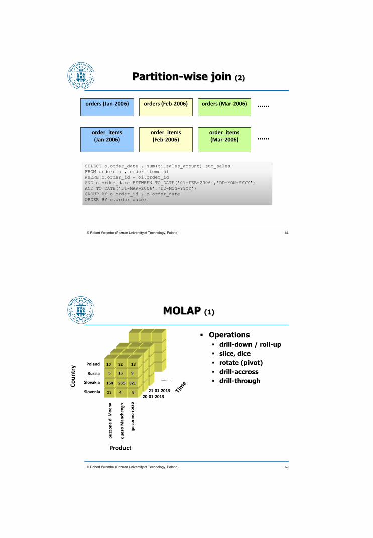
MOLAP (1)
Operations
drill-down / roll-up
slice, dice
rotate (pivot)
drill-accross
drill-through
© Robert Wrembel (Poznan University of Technology, Poland)
20-01-2013
21-01-2013
.........
10
5
150
13
32
16
265
4
13
9
321
8
Product
Poland
Slovakia
Slovenia
Russia
Co
un
try
62
MOLAP (2)
Implementations
N-dim array
Hash table (SQL Server)
BLOB (Oracle)
Quad-tree
K-D-tree
Systems
Cognos PowerPlay (IBM)
Oracle OLAP DML
Hyperion Essbase (Oracle)
MicroStrategy
MS Analysis Services (Microsoft)
SAS OLAP Server
© Robert Wrembel (Poznan University of Technology, Poland) 63
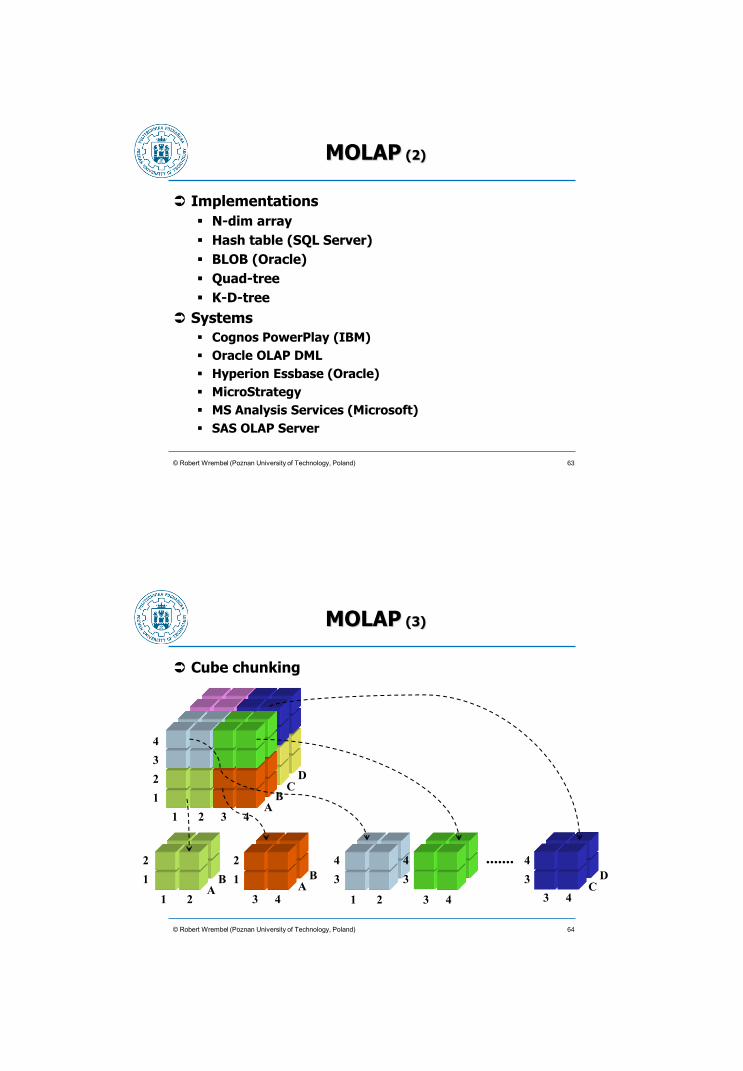
MOLAP (3)
© Robert Wrembel (Poznan University of Technology, Poland)
Cube chunking
.......
1 2 3 4
1
2
3
4
A B
C D
1 2 3 4 1 2 3 4 3 4
1
2
1
2
3
4
3
4
3
4
A B
A B
C D
64

MOLAP (4)
© Robert Wrembel (Poznan University of Technology, Poland)
1 2 3 4
1
2
3
4
C D
A B
Compression - store cells that contain NOT NULL values
compress when % of NULL cells reaches a given threshold (e.g., 40%)
A B
1 2 3 4 1 2
1
2
1
2
3
4
3
4
A B
[1,4,C: value][4,4,D: value]
compression
65
MOLAP (5)
More efficient than ROLAP for aggregate computing
Efficient when a cube contains a few dimension
Loading less efficient than ROLAP
© Robert Wrembel (Poznan University of Technology, Poland) 66
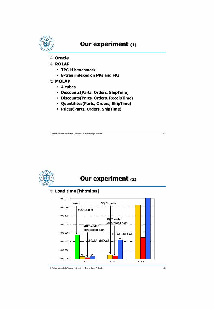
Our experiment (1)
Oracle
ROLAP
TPC-H benchmark
B-tree indexes on PKs and FKs
MOLAP
4 cubes
Discounts(Parts, Orders, ShipTime)
Discounts(Parts, Orders, ReceipTime)
Quantitites(Parts, Orders, ShipTime)
Prices(Parts, Orders, ShipTime)
© Robert Wrembel (Poznan University of Technology, Poland) 67
Our experiment (2)
© Robert Wrembel (Poznan University of Technology, Poland)
Load time [hh:mi:ss]
insert
SQL*Loader
SQL*Loader (direct load path)
ROLAP->MOLAP
SQL*Loader
SQL*Loader (direct load path)
ROLAP->MOLAP
68
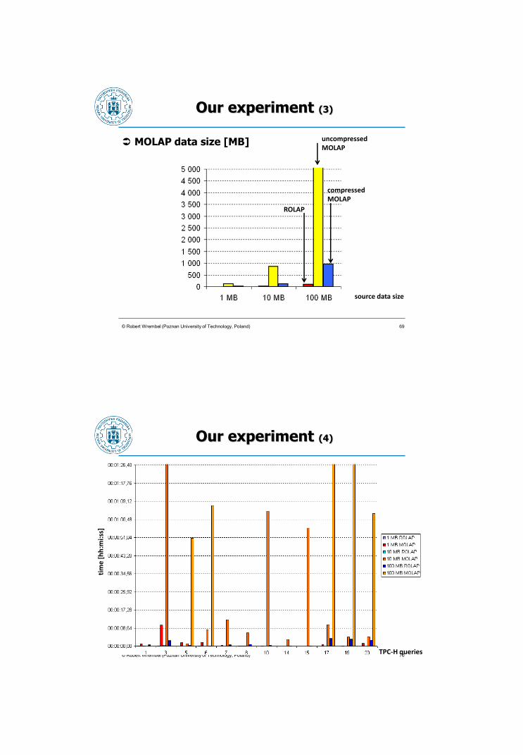
Our experiment (3)
MOLAP data size [MB]
© Robert Wrembel (Poznan University of Technology, Poland)
source data size
ROLAP
compressed MOLAP
uncompressed MOLAP
69
Our experiment (4)
© Robert Wrembel (Poznan University of Technology, Poland) TPC-H queries
tim
e [
hh
:mi:
ss]
70
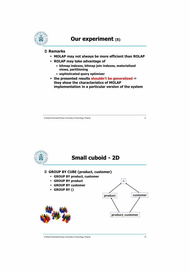
Our experiment (5)
Remarks
MOLAP may not always be more efficient than ROLAP
ROLAP may take advantage of
• bitmap indexes, bitmap join indexes, materialized views, partitioning
• sophisticated query optimizer
the presented results shouldn't be generalized
they show the characteristics of MOLAP implementation in a particular version of the system
© Robert Wrembel (Poznan University of Technology, Poland) 71
Small cuboid - 2D
GROUP BY CUBE (product, customer)
GROUP BY product, customer
GROUP BY product
GROUP BY customer
GROUP BY ()
72 © Robert Wrembel (Poznan University of Technology, Poland)
product, customer
product customer
┴
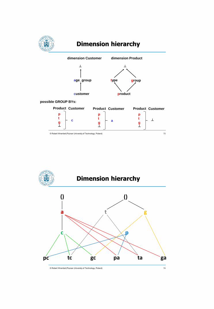
Dimension hierarchy
73 © Robert Wrembel (Poznan University of Technology, Poland)
customer
age_group
┴
dimension Customer
product
type
┴
dimension Product
group
p
t
g
┴
Product Customer
a
p
t
g
┴
Product Customer
c
p
t
g
┴
Product Customer
┴
possible GROUP BYs:
Dimension hierarchy
74 © Robert Wrembel (Poznan University of Technology, Poland)
t a g
() ()
a
c p
pc tc gc pa ta ga
75 © Robert Wrembel (Poznan University of Technology, Poland)
3D rollup
GROUP BY ROLLUP (sklep, produkt, data)
GROUP BY sklep, produkt, data
GROUP BY sklep, produkt
GROUP BY sklep
GROUP BY ()
76 © Robert Wrembel (Poznan University of Technology, Poland)
3D cuboid
GROUP BY CUBE (sklep, produkt, data)
GROUP BY sklep, produkt, data
GROUP BY sklep, produkt
GROUP BY sklep, data
GROUP BY produkt, data
GROUP BY sklep
GROUP BY produkt
GROUP BY data
GROUP BY ()

77 © Robert Wrembel (Poznan University of Technology, Poland)
4D cuboid
product, shop, client, date
product, shop, client product, shop, date shop, client, date product, client, date
product, shop product, client shop, client product, date shop, date client, date
product shop client date
total
Lattice
Cuboid, hypercube
78 © Robert Wrembel (Poznan University of Technology, Poland)
Optimizing GROUP BY
SPD
SP SD PD
S P D
( ) Assumption: for each GROUP
BY scheme one knows:
# unique values
computation cost of a node based on a subordinate node
Optimization goal:
find all grouping schemes so that the total computaiton cost is minimized
20 23
30
9
13
18
16 11 14
3 5 6

79 © Robert Wrembel (Poznan University of Technology, Poland)
Possible Optimization Techniques
Smallest parent
computing a lower level grouping based on the smallest (size) grouping of a lower level
Caching results (in RAM)
a given GROUP BY result is reused for other groupings
group by SPD -> group by SP -> group by S
Amortize disc scans
during one disc scan multiple grouping schemes may be computed
• e.g., assuming that grouping result of SPD is stored on disk, then during wile reading it SP, SD, and PD can be computed
80 © Robert Wrembel (Poznan University of Technology, Poland)
Possible Optimization Techniques
Share sorts
the same sort scheme can be used for computing multiple grouping schemes
Table partitioning
additive functions can be computed based on partial results computed for each partition (parallel processing possible)

81 © Robert Wrembel (Poznan University of Technology, Poland)
The PipeSort Algorithm
Graf traversal:
For each level an arc of the lowest cost is found
SPD
SP SD PD
S P D
( )
20 23
30
9
13 16 11 14
3 5 6
18
SPD
SP
S
()
SPD
SP
P
SPD
SD
D
SPD
PD
GROUP BY execution:
Buffering and reusing results of grouping from a lower level
82 © Robert Wrembel (Poznan University of Technology, Poland)
The PipeHash Algorithm
The concept like in PipeSort
Sorting is implemented by means of hashing

83 © Robert Wrembel (Poznan University of Technology, Poland)
GROUP By Optimization: Summary
Other DW technologies
Parallel and distributed DWs
data (partitions, MVs, indexes) allocation in nodes
load balancing and data redistribution
In-memory/main-memory DWs
optimization of memory usage
compression
DWs in a cloud
assuring scalability
load balancing and data redistribution
high availability
building DWs functionalities on Hadoop/Map Reduce
benchmarking
© Robert Wrembel (Poznan University of Technology, Poland) 84

References
Column storage D.J. Abadi, S.R. Madden, M. Ferreira: Integrating compression and
execution in column-oriented database systems. SIGMOD, 2006
D.J. Abadi, S.R. Madden, N. Hachem: Column-stores vs. row-stores: how different are they really?. SIGMOD, 2008
A. Albano: SADAS - An Innovative Column-Oriented DBMS for Business Intelligence Applications. SADAS Manual
S. Harizopoulos, D. Abadi, P. Boncz: Column-Oriented Database Systems. VLDB tutorial, 2009
M. Stonebraker, D.J. Abadi, A. Batkin, X. Chen, M. Cherniack, M. Ferreira, E. Lau, A. Lin, S.R. Madden, E. O'Neil, P. O'Neil, A. Rasin, N. Tran, S. Zdonik: C-store: a column-oriented DBMS. VLDB, 2005
© Robert Wrembel (Poznan University of Technology, Poland) 85
References
Materialized views S. Ceri, J. Widom: Deriving Production Rules for Incremental View
Maintenance. VLDB, 1991
A. Gupta, I.S. Mumick: Materialized Views: Techniques, Implementations, and Applications. MIT Press, 1999
A. Gupta, I.S. Mumick, V.S. Subrahmanian: Maintaining Views Incrementally. SIGMOD, 1993
S. Kulkarni, M. Mohania.: Concurrent Maintenance of Views Using Multiple Versions. IDEAS, 1999
D. Quass, J. Widom: On-line Warehouse View Maintenance. SIGMOD, 1997
M. Teschke, A. Ulbrich: Concurrent Warehouse Maintenance Without Compromising Session Consistency. DEXA, 1998
S. Samtani, V. Kumar, M. Mohania: Self Maintenance of Multiple Views in Data Warehousing. CIKM, 1999
H. Wang, M. Orlowska, W. Liang: Efficient Refreshment of Materialized Views With Multiple Sources. CIKM, 1999
Y. Zhuge, H. Garcia-Molina, J. Hammer, J. Widom: View Maintenance in Warehousing Environment. SIGMOD, 1995
Y. Zhuge, H. Garcia-Molina, J. Wiener: The Strobe Algorithms for Multi-Source Warehouse Consistency. PDIS, 1996
© Robert Wrembel (Poznan University of Technology, Poland) 86

References
© Robert Wrembel (Poznan University of Technology, Poland)
Small summary data G. Graefe: Fast loads and fast queries. DaWaK, 2009
G. Moerkotte: Small materialized aggregates: A light weight index structure for data warehousing. VLDB, 1998
IBM Netezza Database User’s Guide. IBM Netezza 7.0.x, Oct 2012
Netezza underground: Zone maps and data power. https://www.ibm.com/developerworks/community/blogs/Netezza/entry/zone_maps_and_data_power20?lang=en
Partitioning
P. Furtado: Experimental evidence on partitioning in parallel data warehouses. DOLAP 2004
P. Furtado: Algorithms for Efficient Processing of Complex Queries in Node-Partitioned Data Warehouses. IDEAS 2004
P. Furtado: A Survey of Parallel and Distributed Data Warehouses. IJDWM 5(2), 2009
L. Bellatreche, R. Bouchakri, A. Cuzzocrea, S. Maabout: Horizontal partitioning of very-large data warehouses under dynamically-changing query workloads via incremental algorithms. SAC, 2013
87
References
GROUP BY optimization Agarwal S., Agrawal R., Deshpande M. P., Gupta A., Naughton F. J.,
Ramakrishnan R., Sarawagi S.: On the Computation of Multidimensional Aggregates. VLDB, 1996
Ross K. A., Srivastava D.: Fast Computation of Sparse Datacubes. VLDB, 1997
Beyer K, Ramakrishnan R.: Bottom-Up Computation of Sparse and Iceberg Cubes. SIGMOD, 1999
Wang W., Feng J., Lu H., Xu Yu J.: Condensed Cube: An Effective Approach to Reducing Data Cube Size. ICDE, 2002
Lakshmanan L., Pei J., Han J.: Quotient cube: How to summarize the semantics of a data cube. VLDB, 2002
Chen Z., Narasayya V.: Efficient Computation of Multiple Group By Queries. SIGMOD, 2005
Morfonios K., Ioannidis Y.: CURE for Cubes: Cubing Using a ROLAP Engine. VLDB, 2006
88 © Robert Wrembel (Poznan University of Technology, Poland)