Manuscript prepared for Earth Syst. Sci. Datawith version 2015/09/17 7.94 Copernicus papers of the LATEX class copernicus.cls.Date: 2 March 2016

CPLFD-GDPT5: High-resolution gridded dailyprecipitation and temperature dataset for two largestPolish river basinsTomasz Berezowski1, Mateusz Szczesniak1, Ignacy Kardel1, Robert Michałowski1,Tomasz Okruszko1, Abdelkader Mezghani2, and Mikołaj Piniewski1,3

1Department of Hydraulic Engineering, Warsaw University ofLife Sciences, Nowoursynowska166, 02-787 Warsaw, Poland.2Norwegian Meteorological Institute, Henrik Mohns Plass 1,0313 Oslo, Norway3Potsdam Institute for Climate Impact Research, Telegrafenberg, 14473 Potsdam, Germany.

Correspondence to:T. Berezowski (t.berezowski@levis.sggw.pl)

Abstract. The CHASE-PL Forcing Data - Gridded Daily Precipitation & Temperature Dataset -

5km (CPLFD-GDPT5) consists of 1951-2013 daily minimum and maximum air temperatures and

precipitation totals interpolated onto a 5 km grid based on daily meteorological observations from

Institute of Meteorology and Water Management (IMGW-PIB; Polish stations), Deutscher Wetter-

dienst (DWD, German and Czech stations), ECAD and NOAA-NCDC(Slovak, Ukrainian and Be-5

larus stations). The main purpose for constructing this product was the need for long-term aerial

precipitation and temperature data for earth-system modelling, especially hydrological modelling.

The spatial coverage is the union of Vistula and Odra basin and Polish territory. The number of

available meteorological stations for precipitation and temperature varies in time from about 100

for temperature and 300 for precipitation in 1950’s up to about 180 for temperature and 700 for10

precipitation in 1990’s. The precipitation dataset was corrected for snowfall and rainfall under-catch

with the Richter method. The interpolation methods were: kriging with elevation as external drift for

temperatures and indicator kriging combined with universal kriging for precipitation. The kriging

cross-validation revealed low root mean squared errors expressed as a fraction of standard deviation

(SD): 0.54 and 0.47 for minimum and maximum temperature, respectively and 0.79 for precipita-15

tion. The correlation scores were 0.84 for minimum temperatures, 0.88 for maximum temperatures

and 0.65 for precipitation. The CPLFD-GDPT5 product is consistent with 1971-2000 climatic data

published by IMGW-PIB. We also confirm good skill of the product for hydrological modelling by

performing an application using the Soil and Water Assessment Tool (SWAT) in the Vistula and

Odra basins.20

Link to the dataset: http://data.3tu.nl/repository/uuid:e939aec0-bdd1-440f-bd1e-c49ff10d0a07

1

1 Introduction

High resolution aerial precipitation and air temperature data is becoming more and more desired as

input or verification data for distributed earth-system modelling. Certainly, one of the most demand-

ing branch for these data is distributed hydrological modelling. Rainfall-runoff models, e.g.: SWAT25

(Arnold et al., 1998), WetSpa (Liu and De Smedt, 2004) or TOPMODEL (Beven et al., 1995), rely

on precipitation as a driver for hydrological processes. Similarly, integrated models, e.g. MIKE SHE

(Abbott et al., 1986), HydroGeoSphere (Brunner and Simmons, 2012) or ParFLOW (Kollet and Maxwell,

2006), and channel and floodplain hydrodynamical models, e.g. LISFLOOD-2D (Bates and De Roo,

2000) can use precipitation data as a boundary condition. There are also numerous applications for30

precipitation in hydrological engineering, e.g., peak flowat a given return period or runoff coeffi-

cient estimations. Applicability of temperature data in hydrological modelling is also very impor-

tant, although, less straightforward. Temperature is often used as a variable in sub-components of

hydrological models. Models like WetSpa, SWAT, SRM (Martinec, 1975) or HydroGeoSphere use

temperature for snowmelt estimation with the degree-day model. Several models use air tempera-35

ture and ancillary variables to estimate potential evapotranspiration (e.g. Hargreaves, 1975) or actual

evapotranspiration (e.g. Wang et al., 2007). These models can be applied independently from hy-

drological models in order to generate evapotranspirationseries but can be also implemented in the

models source code (e.g. Hargreaves in SWAT).

Global datasets which include (sub-)daily gridded precipitation and temperature (Sheffield et al.,40

2006; Dee et al., 2011; Schamm et al., 2014; Weedon et al., 2014) are available in a range of spa-

tial resolutions, with typically highest resolution of 0.25x0.25 degrees, which is equivalent to 28x28

km at the equator and 28x14 km at the 60 degrees North. Numerous applications of these datasets are

found for large-scale hydrological modelling (Haddeland et al., 2011; Li et al., 2013; Abbaspour et al.,

2015). However, the aforementioned spatial resolution is often not high enough when the study area45

is smaller than one grid cell of the data. For this reason local meteorological gridded datasets are

continuously appearing, at countrywide or regional scale (Jones et al., 2009; Rauthe et al., 2013;

Isotta et al., 2014; Keller et al., 2015). So far no high resolution gridded dataset exists neither for

Vistula nor Odra basin nor for Polish territory, except a partial cover by the CARPATCLIMproject

(Spinoni et al., 2015):::::::::::::::::::::

(Spinoni et al., 2015) and:::::::

HYRAS::::::::::::::::::::::

(Frick et al., 2014) projects. The advantage50

of the regional datasets is their finer spatial resolution than in the global datasets, usually between

5x5 km and 1x1 km. Hence, they are better suitable for local-scale modelling (e.g. hydrological

modelling) than the coarser-resolution global datasets (Berezowski et al., 2015a).

The mentioned above regional gridded dataset are constructed by interpolating observations from

national meteorological networks. However, no clear guideline exists for selecting optimal method55

for spatial interpolation of meteorological variables. Ingeneral the geostatistical (kriging) and in-

verse distance weighted (IDW) methods are preferable for seasonal and daily rainfall interpolation

over Thiessen polygons, polynomial interpolation or otherdeterministic methods (Ly et al., 2013).

2

An earlier study by (Szczesniak and Piniewski, 2015) showed that kriging interpolation of precip-

itation for several meso-scale basins in Poland outperformed IDW and Thiessen polygons in skill60

for hydrological modelling. Indeed, kriging is recently often used as the interpolation method for

precipitation and air temperature with satisfactory results quantified by correlation coefficients or

root mean squared errors (Carrera-Hernández and Gaskin, 2007; Hofstra et al., 2008; Ly et al., 2011;

Herrera et al., 2012). Each of these studies, however, use different flavours of kriging, that can be:

ordinary kriging (assumes constant mean), universal kriging (removal of trend based on the spatial65

coordinates), kriging with external drift (mean is dependent on external variable, e.g. elevation map),

co-kriging (estimates a variable based on it’s values and values of other variables) and others. Again,

selection of the most appropriate kriging method is variable dependent (by studying phenomena re-

sponsible for observations of the variable, e.g. relationswith elevation) and case-study dependent

(by investigating whether any trend is observed at given spatial and temporal scale, e.g. seasonal and70

geographical relations with climate).

In this study we show the work-flow for constructing the CHASE-PL Forcing Data - Gridded Daily

Precipitation & Temperature Dataset - 5km (CPLFD-GDPT5) product. The CPLFD-GDPT5 product

is aimed at providing input data for earth-system modelling, especially hydrological modelling. The

work-flow description is accompanied by detailed verification of the product, consistency check of75

the product with long-term climatic maps and description ofthe product applicability. Objective of

this study is to give transparent information about the CPLFD-GDPT5 details for users. We also

believe that the presented herein work-flow can be a guideline for other regional meteorological

interpolation studies.

2 Data processing and methods80

2.1 Temporal and spatial representation of the CPLFD-GDPT5

The temporal range for the CPLFD-GDPT5 product is from 1951-01-01 to 31-12-2013 in daily

resolution, in total 23011 days. In the source data some records since 1940 were available, however,

the network of meteorological stations was too sparse for reasonable interpolation results before

1951.85

The spatial extent of the CPLFD-GDPT5 product is the union ofVistula and Odra basins and the

Polish territory (Figure 1). The spatial resolution is 5 km square grid. We used projected coordinate

system PUWG 1992 (EPSG:2180), which has an advantage of being valid for our entire area of

interest. The coordinate system PUWG 1992 has distortions varying longitudinally ranging from

-70 cm/km (western study area) to 90 cm/km (eastern study area), which are negligible at 5 km grid90

resolution. Moreover, PUWG-1992 is easily re-projected toother coordinate system, because it is

based on the Geodetic Reference System ’80 (GRS 80) ellipsoid (GRS 80 is almost the same as the

World Geodetic System ’84 - WGS 84 ellipsoid).

3

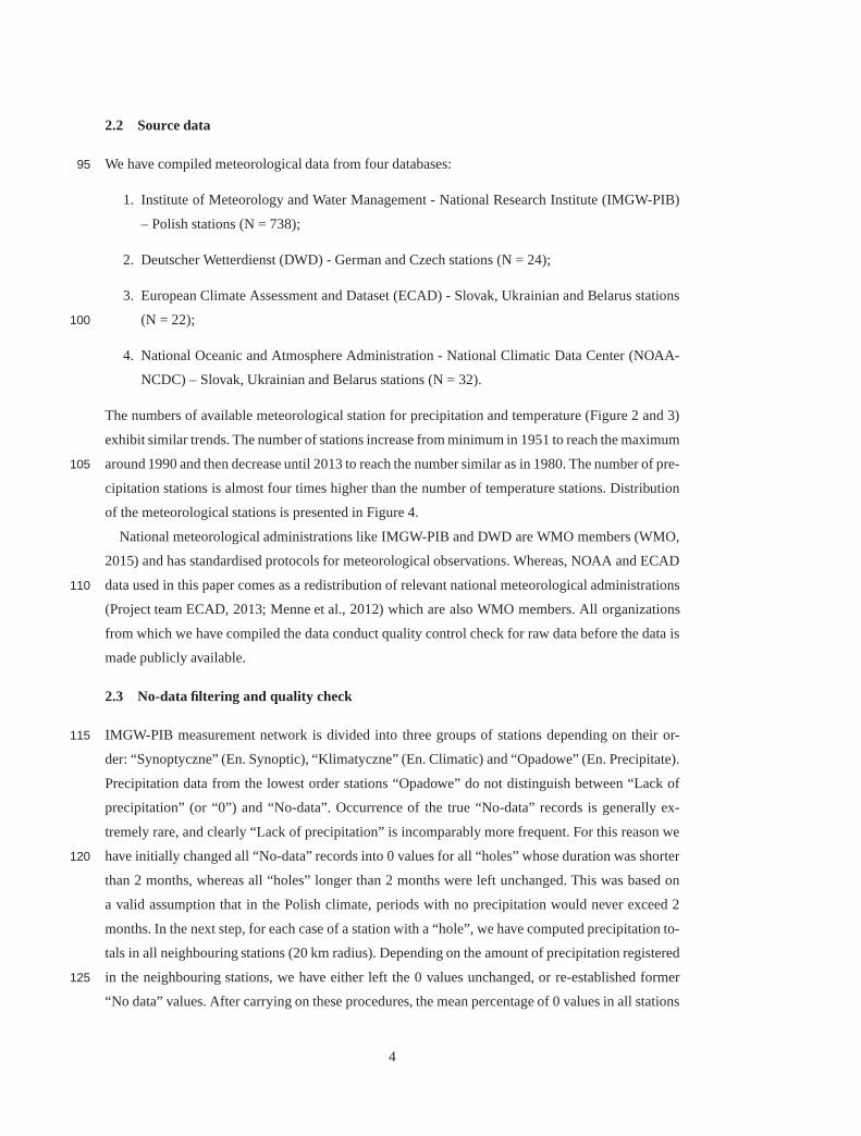
2.2 Source data

We have compiled meteorological data from four databases:95

1. Institute of Meteorology and Water Management - NationalResearch Institute (IMGW-PIB)

– Polish stations (N = 738);

2. Deutscher Wetterdienst (DWD) - German and Czech stations(N = 24);

3. European Climate Assessment and Dataset (ECAD) - Slovak,Ukrainian and Belarus stations

(N = 22);100

4. National Oceanic and Atmosphere Administration - National Climatic Data Center (NOAA-

NCDC) – Slovak, Ukrainian and Belarus stations (N = 32).

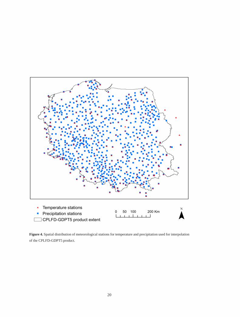
The numbers of available meteorological station for precipitation and temperature (Figure 2 and 3)

exhibit similar trends. The number of stations increase from minimum in 1951 to reach the maximum

around 1990 and then decrease until 2013 to reach the number similar as in 1980. The number of pre-105

cipitation stations is almost four times higher than the number of temperature stations. Distribution

of the meteorological stations is presented in Figure 4.

National meteorological administrations like IMGW-PIB and DWD are WMO members (WMO,

2015) and has standardised protocols for meteorological observations. Whereas, NOAA and ECAD

data used in this paper comes as a redistribution of relevantnational meteorological administrations110

(Project team ECAD, 2013; Menne et al., 2012) which are also WMO members. All organizations

from which we have compiled the data conduct quality controlcheck for raw data before the data is

made publicly available.

2.3 No-data filtering and quality check

IMGW-PIB measurement network is divided into three groups of stations depending on their or-115

der: “Synoptyczne” (En. Synoptic), “Klimatyczne” (En. Climatic) and “Opadowe” (En. Precipitate).

Precipitation data from the lowest order stations “Opadowe” do not distinguish between “Lack of

precipitation” (or “0”) and “No-data”. Occurrence of the true “No-data” records is generally ex-

tremely rare, and clearly “Lack of precipitation” is incomparably more frequent. For this reason we

have initially changed all “No-data” records into 0 values for all “holes” whose duration was shorter120

than 2 months, whereas all “holes” longer than 2 months were left unchanged. This was based on

a valid assumption that in the Polish climate, periods with no precipitation would never exceed 2

months. In the next step, for each case of a station with a “hole”, we have computed precipitation to-

tals in all neighbouring stations (20 km radius). Dependingon the amount of precipitation registered

in the neighbouring stations, we have either left the 0 values unchanged, or re-established former125

“No data” values. After carrying on these procedures, the mean percentage of 0 values in all stations

4

belonging to the order “Opadowe” was equal to 52 %. In comparison, the respective numbers for

two other orders of stations that were free of such problems (“Synoptyczne” and “Klimatyczne”),

were equal to 51 and 55 %, respectively, which shows that the applied procedure did not alter the

distribution of dry days in time series.130

We have also removed suspicious values from the temperaturetime series. There were two cases of

suspiciously high values of temperature at two stations, both with periods of these incorrect values no

longer than a month. This data was removed from the dataset. Possibly the errors may be attributed

to the failure of the measuring device. In addition daily andmonthly values of precipitation and

maximum and minimum temperatures at IMGW-PIB stations werecompared with climatic records135

for Poland to check for outlying values. Moreover several NOAA stations with suspiciously high

values of precipitation with constantly repeating exact the same values were removed.

2.4 Rainfall and snowfall under-catch correction

Local precipitation measured in a rain gauge is not representative for aerial precipitation. This is

due to various factors, e.g.: wind speed, rain gauge shielding, or precipitation type. Several models140

for correcting precipitation for under-catch were developed. In Poland an empirical model proposed

by Chomicz (1976) is often used. The Chomicz (1976) model considers only liquid precipitation

and has parameters available only within Polish borders. Hence, we had to used another model,

that is valid internationally and accounts for both solid and liquid precipitation. We have chosen the

Richter (1995) model for correcting snowfall and rainfall under-catch, which is recognized by WMO145

(Goodison et al., 1998). The Rainfall and snowfall under-catch correction is applied in the following

steps:

1. Mean daily air temperature [◦C] is calculated for all precipitation stations, as:t= (tn+ tx)/2.

The tn and tx are the minimum and maximum daily temperatures [◦C] obtained from our

CPLFD-GDPT5 product (see Section 2.5.1). For the calculations we have usedtn andtx val-150

ues from a grid cell containing respective meteorological precipitation station. We could not

use the average temperatures measured at the stations because the latter were not recorded sys-

tematically at the majority of the stations. Neither, we didnot want to use a blended approach

(use measured temperature if available, otherwise use interpolated), because this would be

harmful for calculation consistency.155

2. Measured precipitation is classified based on mean daily temperature, as:

(a) snow ift < 1.0◦C,

(b) mixed snow and rain ift≥ 1.0◦C ∧ t < 2.0◦C,

(c) or rain if t≥ 2.0◦C.

5

3. The corrected precipitation [mm] is calculated based on Richter (1995) formulae asp= bpǫ,160

wherep is the measured precipitation total [mm],b is the coefficient [-] for the influence of

wind exposition of the measurements site, andǫ is a seasonally varying empiric coefficient [-]

for the precipitation type (snow, mixed snow and rain, or rain). Range ofb andǫ values used

in this paper is available in Richter (1995). The values ofb were set as for “medium shielding”

for all stations apart from those in the mountains or close tothe coast, whereb were set as for165

“low shielding” (Figure 5). The rationale behind assigningdifferent values ofb for different

location lays in the fact that wind speed is generally higherin mountains and at the seaside

than in the lowlands.

2.5 Interpolation

Our meteorological observations with spatial coordinatesafter pre-processing steps described above170

(Sections 2.2-2.4) were interpolated with two different kriging methods. Minimum and maximum

temperatures were interpolated with the kriging with external drift and precipitation with universal

kriging. The exponential variogram model was used in each case with the variogram parameters

estimated automatically for each daily kriging with the weighted least squares fit (Pebesma, 2014).

The block kriging approach was used with the block size equalto the output square grid size, i.e., 5175

km. Computations were conducted in the R software (R Core Team, 2015) with the “gstat” package

(Pebesma, 2004).

2.5.1 Temperature kriging

Both minimum and maximum temperatures were interpolated inthe same way. Kriging with external

drift was used in order to account for the temperature variability with elevation. This approach was180

used in other similar studies (e.g. Hattermann et al., 2005;Haylock et al., 2008). The external drift

variable was elevation [m] obtained from the SRTM DEM aggregated to 5 km grid. In order to

remove the “No-data” values from the SRTM data the elevationof seas and oceans was relabelled to

0.0 m.

2.5.2 Precipitation kriging185

Precipitation was interpolated using a two-step approach combining the universal kriging of the

precipitation data (first step) with the indicator kriging of the precipitation occurrence data (sec-

ond step). This approach was selected due to giving good results with a similar problem (e.g.

Herrera et al., 2012). Universal kriging was chosen becausethe trend was not removed from the

precipitation data beforehand. Indicator kriging was applied on binary data in order to allow reduc-190

ing the smoothing effect of around zero value zones. The daily precipitation totalsp in each station

6

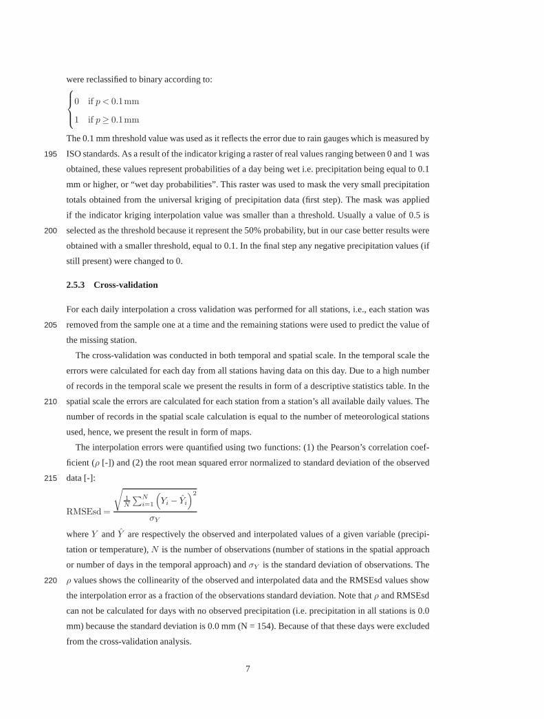
were reclassified to binary according to:

0 if p < 0.1mm

1 if p≥ 0.1mm

The 0.1 mm threshold value was used as it reflects the error dueto rain gauges which is measured by

ISO standards. As a result of the indicator kriging a raster of real values ranging between 0 and 1 was195

obtained, these values represent probabilities of a day being wet i.e. precipitation being equal to 0.1

mm or higher, or “wet day probabilities”. This raster was used to mask the very small precipitation

totals obtained from the universal kriging of precipitation data (first step). The mask was applied

if the indicator kriging interpolation value was smaller than a threshold. Usually a value of 0.5 is

selected as the threshold because it represent the 50% probability, but in our case better results were200

obtained with a smaller threshold, equal to 0.1. In the final step any negative precipitation values (if

still present) were changed to 0.

2.5.3 Cross-validation

For each daily interpolation a cross validation was performed for all stations, i.e., each station was

removed from the sample one at a time and the remaining stations were used to predict the value of205

the missing station.

The cross-validation was conducted in both temporal and spatial scale. In the temporal scale the

errors were calculated for each day from all stations havingdata on this day. Due to a high number

of records in the temporal scale we present the results in form of a descriptive statistics table. In the

spatial scale the errors are calculated for each station from a station’s all available daily values. The210

number of records in the spatial scale calculation is equal to the number of meteorological stations

used, hence, we present the result in form of maps.

The interpolation errors were quantified using two functions: (1) the Pearson’s correlation coef-

ficient (ρ [-]) and (2) the root mean squared error normalized to standard deviation of the observed

data [-]:215

RMSEsd =

√

1

N

∑N

i=1

(

Yi − Yi

)2

σY

whereY andY are respectively the observed and interpolated values of a given variable (precipi-

tation or temperature),N is the number of observations (number of stations in the spatial approach

or number of days in the temporal approach) andσY is the standard deviation of observations. The

ρ values shows the collinearity of the observed and interpolated data and the RMSEsd values show220

the interpolation error as a fraction of the observations standard deviation. Note thatρ and RMSEsd

can not be calculated for days with no observed precipitation (i.e. precipitation in all stations is 0.0

mm) because the standard deviation is 0.0 mm (N = 154). Because of that these days were excluded

from the cross-validation analysis.

7

3 Validation225

3.1 Cross-validation of precipitation

The dailyρ and RMSEsd statistics for precipitation shows that 75% ofρ values are higher than

0.47 and RMSEsd values are lower than 0.93, respectively (Table 1). Medianρ is 0.65 and median

RMSEsd is 0.79. Majority of the RMSEsd values are not exceeding one standard deviation and

nearly allρ values are positive.230

The median of daily RMSEsd values aggregated in years is negatively correlated (-0.72) with the

number of available stations (Figure 7), sharply decreasing as the number of stations increases and

reaching an equilibrium in 1980s. This suggests that the kriging errors are dependent on the density

of the observation network. We also found that the interpolation results before 1960 are associated

with higher uncertainty (Figure 7).235

When considering the RMSEsd calculated spatially for all stations the results show a clear pattern

of higher errors at the edge of the interpolation area, particularly in Belarus, Ukraine and Slovakia

(Figure 6). Notably, most of the stations with high errors come from other sources than IMGW-PIB.

Indeed, stations at the edge of the interpolation area, which are managed by IMGW-PIB or DWD

do not show the higher errors (cf. NE and W boundary). The median RMSEsd in the spatial scale is240

0.50. Analogous situation is obtained forρ spatial pattern in meteorological station (Figure 6) with

the medianρ equals to 0.87.

A similar interpolation study was conducted by Ly et al. (2011). In their study the error was quan-

tified by RMSE not normalized to standard deviation, thus, the units were mm. After recalculation of

our RMSEsd back to RMSE the values show similar ranges as in Lyet al. (2011), with interquartile245

range 0.5-2.5 mm and 97.5 percentile of 5.5 mm suggesting that our errors are within an acceptable

range.

3.2 Cross-validation of temperature

The statistics of daily RMSEsd shows the median equal to 0.54for the minimum temperature and

0.47 for maximum temperature (Table 1). Nearly all the RMSEsd values in both cases do not exceed250

one standard deviation and theρ values are positive. The dailyρ statistics for minimum and max-

imum temperature show that 75% ofρ values are above 0.77 for minimum temperature and above

0.86 for maximum temperature. The median ofρ is 0.84 for the minimum temperature and 0.88 for

the maximum temperature.

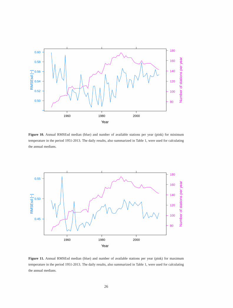
The median of daily RMSEsd values for minimum temperature aggregated in years is not corre-255

lated (0.00) with the number of available stations (Figure 10). The RMSEsd is reaching a minimum

in 1970s. Since then it is however gradually increasing (at asmall rate), which does not seem to be

related to changes in the number of available stations. The situation is only slightly different for the

maximum temperatures (Figure 11), for which correlation with the number of stations is weak (0.22).

8

Although the lowest RMSEsd can be observed for the 1960s, since then a gradual increase (again,260

at a small rate and) can be observed. It should also be noted that the range of RMSEsd is not very

wide, in general (0.48-0.6 for the minimum temperature and 0.42-0.5, neglecting one outlier, for the

maximum temperature). Overall, it seems that our kriging errors for temperature are not dependent

on the density of the observation network. However, as in thecase of precipitation interpolation the

results before 1960 are associated with higher uncertainties.265

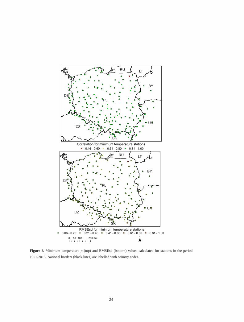
When analysing the RMSEsd results calculated spatially forall stations the minimum tempera-

ture shows a rather uniformly distributed values with a few outliers located at the boundary of the

interpolation area, mostly in the mountains (southern border, Figure 8). Analogous situation is ob-

served for maximum temperatures (Figure 9). The median RMSEsd in spatial scale is equal to 0.17

for minimum temperature and 0.10 for maximum temperature. Analogous situation is observed for270

ρ spatial pattern for meteorological station with the medianρ equal to 0.99 both for minimum and

maximum temperature.

A similar interpolation exercise was conducted by Carrera-Hernández and Gaskin (2007). In their

study the error was quantified byρ2. Ranges ofρ2 obtained in their study were, for the maximum

temperature: 0.73-0.88 and for the minimum temperature: 0.68-0.96. These results are very similar275

to ours (after recalculatingρ to ρ2), suggesting good quality of the gridded temperature dataset.

4 Consistency with climatic data

The precipitation and minimum and maximum temperature gridded products were analysed for con-

sistency with long term climatic data. Since the majority ofour product spatial coverage is in Poland

we have used long term climatic maps from Polish meteorological service (IMGW-PIB) for compar-280

ison. The IMGW-PIB maps were developed for the period 1971-2000 and include: precipitation to-

tals, 5% minimum temperature and 95% maximum temperature (IMGW-PIB, 2015). For purpose of

the comparison analysis we have constructed analogous mapsfrom a 1971-2000 subset of CPLFD-

GDPT5 by: (1) averaging the annual precipitation totals, (2) calculating 5% quantile from the daily

minimum temperatures, (3) calculating 95% quantile from the daily maximum temperatures.285

This comparison analysis have several limitations. Both products were constructed by different

interpolation methods and using data from different collection of meteorological stations. Another

limitation in this comparison is that input data were subjected to different preprocessing steps, of

which the most important is the different rainfall and snowfall under-catch correction. Due to these

limitations we do not except to have an ideal match between our and IMGW-PIB climatic data.290

However, we expect that ranges and diversity of climatic data would present similar spatial patterns

if our gridded product was constructed properly.

The latitudinal precipitation totals pattern with 750 mm inthe north, decrease in centre and maxi-

mum in the south was well preserved by CPLFD-GDPT5 product (Figure 12). Range of precipitation

9

totals in CPLFD-GDPT5 in Poland (1971-2000) was from 552 to1402 mm, whereas, for the IMGW-295

PIB the range was from 450-500 mm to 1250-1300 mm. The centralregions with the lowest (450-500

mm) precipitation were overestimated in CPLFD-GDPT5. Similarly, CPLFD-GDPT5 overestimates

by about 100 mm the highest precipitations in the central-southern region. We believe this discrep-

ancy is due to rainfall and snowfall under-catch correctionused in our study, which assigns higher

correction factors to snowfall than to rainfall.300

The longitudinal 5% minimum temperatures pattern with -6◦C in the east, -12◦C in the west

and the minimum (-13◦C) in the central-south was well preserved by CPLFD-GDPT5 (Figure 13).

Range of 5% minimum temperatures in CPLFD-GDPT5 in Poland (1971-2000) was from -15.1 to

-5.8◦C, whereas, for the IMGW-PIB the range was from -14 - -13◦C to -5 - -6◦C. We do not identify

any substantial difference in the temperature patterns in both data sources except an island of -6 -305

-7◦C located in the central-eastern region that was not presentin CPLFD-GDPT5. We believe that

this and other, smaller discrepancies are a result of methodological differences in constructing of

both data sources, especially the use of different meteorological stations data sets.

The complex latitudinal pattern in the north, the longitudinal pattern in the centre and south and

the elevation dependent pattern in south (Sudeten and Carpathian Mountains) for 95% maximum310

temperatures was well preserved by CPLFD-GDPT5 (Figure 14). Range of 95% maximum tem-

peratures in CPLFD-GDPT5 in Poland (1971-2000) was from 15.7 to 28.0◦C, whereas, for the

IMGW-PIB the range was from 18-19◦C to 27-28◦C. Again, we do not identify any substantial dif-

ference in the temperature patterns in both data sources. However, CPLFD-GDPT5 underestimates

the temperature in the peaks of Carpathian Mountains by about 2◦C. More clutter is also observed315

in our product in entire region, especially in the south (mountains). We believe that these discrep-

ancies are a result, as in the previous cases, of methodological differences in constructing of both

data sources, especially the use of high resolution and detailed elevation data in our study, including

differences in the available stations used.

5 Applicability320

This product was developed with the purpose of its further (re)use for earth-system modelling, and

in particular for hydrological modelling and climate impact studies. Spatial resolution (5 km) of

CPLFD-GDPT5 ensures that it will be useful not only for regional studies, where generally lower

resolution data would be appropriate, but also for modelling in local scale, where high spatial reso-

lution is necessary to capture the variability.325

As an example application of CPLFD-GDPT5 for hydrological modelling, we have set up, cali-

brated and validated the SWAT model for the Vistula and Odra basins (Piniewski et al., submitted).

SWAT is a process-based, semi-distributed, continuous-time hydrological model that simulates the

movement of water, sediment and nutrients on a catchment scale with a daily time step (Arnold et al.,

10

1998). Apart from the CPLFD-GDPT5 precipitation and temperatures that are major input data, the330

SWAT setup of the Vistula and Odra basins uses various spatial input data such as topography,

hydrography, land cover and soils, all with quite complex parametrisations. Figure 15a shows spa-

tial variability of mean annual potential evapotranspiration (PET) calculated in SWAT using the

Hargreaves (1975) method, relying on our minimum and maximum temperature data. In the Har-

greaves method PET is proportional to mean temperature (approximated by the arithmetic mean335

of minimum and maximum temperature) and the difference between maximum and minimum tem-

perature (being a proxy of solar radiation).::

As:::::::::

illustrated::

in:::::

many:::::::

studies,:::

the:::::::::

Hargreaves:::::

PET::

is

:::::

highly:::::::::

correlated::

to:::::

other:::::::

methods:::

for:::::

PET:::::::::

estimations:::::::::::::::::

(Lu et al., 2005) and:::

to::::

PET:::::::::::

observations

:::::::::::::::::::::::::

(Hargreaves and Allen, 2003) .:::::::::

Moreover,:

it::::

was:::::

found::::::::::

particularly::::::

useful:::

for:::::

SWAT:::::::::

modelling:::

by

:::::::::

decreasing::

the::::::::

observed::::

PET:::::::::

estimation::::

error:::::

when::::::::

compared::

to:::

the::::::::::::::

Penman-Monteith::::

PET:::::::::

estimation340

::::::::::::::::::::

(Earls and Dixon, 2008) .:

Spatial pattern in simulated PET not surprisingly follows largely the pat-

tern of maximum temperature (Figure 14).

PET constitutes an upper bound for actual evapotranspiration, which is another variable simulated

in SWAT, crucial for the process of model calibration, typically performed using measured discharge

data. Figures 15b-c show two examples of calibration plots illustrating simulated (95 percent predic-345

tion uncertainty band and one simulation with the highest value of objective function) and measured

daily stream flow from the Vistula and Odra SWAT model developed in Piniewski et al. (submitted).

The gauges were selected to demonstrate high simulation skill of CPLFD-GDPT5 across a range

of scales: the Odra catchment upstream of Gozdowice has 110,000 km2, while the Drweca river

upstream of Rodzone has 1700 km2. Both the positive visual inspection of the hydrograph and the350

high values of objective functions (e.g. coefficient of determination equal to 0.81 and 0.71, respec-

tively, and percent bias of 1.4 and -5.8%, respectively) confirm the usefulness and the quality of the

developed interpolation product. Piniewski et al. (submitted) also showed that precipitation station

density (a proxy for kriging error) is positively correlated with the values of goodness-of-fit measures

across a set of 80 calibration catchments. Therefore, it is recommended that station density should355

be always checked prior to the direct use of CPLFD-GDPT5 for hydrological modelling applications

in a given study area.

CPLFD-GDPT5 could also be well-suited as an observation-based reference dataset for bias cor-

rection of GCM/RCM climate projections, in the same way as the WFD-ERA40 served as the ref-

erence for bias correction at the global scale using the ISI-MIP approach (Hempel et al., 2013)360

or as the SPAIN02 dataset (Herrera et al., 2015) served for bias correction of EURO-CORDEX

models at the regional scale (Casanueva et al., 2015). The potential for further use of bias cor-

rected climate projections (in combination with other requested data sets) in model impact studies

is huge and includes such fields as water, agriculture, biomass, coastal infrastructure, and health

(Warszawski et al., 2014).365

11

6 Data access

The CPLFD-GDPT5 product is available in NetCDF and GeoTIFF formats. The gridded structure

of the data and the NetCDF and GeoTIFF data format ensure thatit will be easily processed in GIS

and data analysis software (e.g. R for both NetCDF and GeoTIFF; list of NetCDF manipulation

software: http://www.unidata.ucar.edu/software/netcdf/software.html). We provide some example R370

scripts that allow to read the data and conduct some basic processing (Appendix 1).

The data are publicly available in the 3TU.Datacentrum repository under the DOI = 10.4121/uuid:e939aec0-

bdd1-440f-bd1e-c49ff10d0a07 (Berezowski et al., 2015b).The NetCDF files naming convention is

VariableForTimeStep.nc. Every NetCDF file is accompanied by an additional description in a *.txt

file and follows the CF-1.0 convention.TimeStepcan be: Days, Months or Years.Variablecan be:375

Tmin/Tmax for minimum/maximum air temperature [◦C] or Preci for precipitation [kg m−2]. Each

daily grid for precipitation or temperature is also stored as a separate GeoTIFF file. The naming con-

vention for GeoTIFF is:prefixYYYYMMDD.tif, with prefixbeing: “pre” for precipitation, “tmin”

for minimum temperature and “tmax” for maximum temperature; whereas, YYYYMMDD is the

date format.380

7 Conclusions

We have constructed a 5 km gridded product of daily precipitation, minimum and maximum air tem-

perature intended primarily for use as input data for local and regional scale modelling. The spatial

extent of the product is the union of Odra and Vistula basins and the border of Poland. The input

data for interpolation originates from meteorological stations managed by many organizations. The385

stations are located in central Europe (western Belarus, northern Czech Republic, eastern Germany,

western Ukraine, entire Poland and northern Slovakia). Various preprocessing steps were introduced

in order to filter missing data and correct the precipitationfor under-catch. The quality of the product

is assessed by cross-validation procedure conducted parallel with the kriging interpolation. The cross

validation shows high correlations and root mean squared errors lower than one standard deviation390

of the observations in all three interpolated variables. However, some particular stations located at

the border of the study area show slightly higher errors and lower correlations. We also evaluated

the consistency of our products with climatic data providedby Polish meteorological organization

(IMGW-PIB). The consistency check confirms the high qualityof the products , with only small

differences resulting from different methodologies and number of selected stations across the re-395

gion. Finally, we show an example application of the griddedproduct for hydrological modelling

in SWAT. The results show very good discharge modelling efficiency in both a small and a large

catchment, which shows that the dataset serves its purpose across a wide range of scales. The high

resolution gridded data set will certainly add value when used as reference in bias-adjustment of

12

regional climate model results (e.g. EURO-CORDEX within the CORDEX Initiative) by providing400

more reliable climate projections for Poland.

The dataset is provided in GeoTIFF and NetCDF format in orderto provide ease of access for

most of the modelling community. Nonetheless, we provide sample R scripts for managing the data

in an appendix.:

:::

The::::::

herein::::::::

presented:::::::

data-set:::

and::::::::

methods::::

have::::::

several:::::::

aspects::

of::::::

further::::::::

research.::

It:::::

would:::

be405

::::::::

interesting:::

to:::::::

compare:::

the:::::::

data-set::::

with:::::

other:::::::

data-sets::

of::::::

lower::::::::

resolution::::

(e.g.:::::::

EOBS)::

in:::::

order::

to

::::

show:::

its:::

true::::::

added::::

value:::

for::::

high:::::::::

resolution:::::::::::

hydrological:::::::::

modelling.:::::::::

Moreover,:::

the:::::::::

comparison:::

of

::

the::::::::::

Hargreaves::::

PET,::::::::

estimated:::::

with::

the::::::::::::::

CPLFD-GDPT5:::::::::::

temperatures,:::::

could:::

be::::::

further::::::::::

investigated

::

in::::

scope:::

of::::

other::::

PET:::::::::

estimation:::::::

methods::::

(e.g.:::::::::::::::

Penman-Monteith)::::

and:::::::::::

observations.::::

Last,:::

we::::::

believe

:::

that::::

there::

is::::

still::::

space::

to:::::::

improve:::

the:::::::::::

interpolation:::::::

methods::

by::::::

testing:::::

other::::::::::

interpolation::::::::::

algorithms.410

:::

The::::::::::::::

CPLFD-GDPT5::::::

product::::

was:::::::::

constructed:::

for:::

the::::::

period::::

1951:

-:::::

2013.::::

The:::

new:::::::::::::

meteorological

:::

data::::

and:::::

novel::::::::::

approaches::

to:::::::::::

interpolation:::::::::

algorithms:::

are:::::::::::

continuously:::::::::

appearing.:::::::

Hence,:::

we:::

are

:::::::

planning::

to::::::

update:::

the:::::::

product::::

both:::

by:::::::::

extending:::

the::::

time::::

span::::

and:::

by::::::

testing::::

new:::::::::::

interpolation

:::::::::

algorithms.::::

The::::::::

extension::

is::::::

planned:::

on:

a:::::::::

three-year::::

basis.415

Appendix A: A script example for processing the .tif and .nc files in R(appendixA.pdf)

Acknowledgements.Support of the project CHASE-PL (Climate change impact assessment for selected sectors

in Poland) of the Polish–Norwegian Research Programme operated by the National Centre for Research and

Development (NCBiR) under the Norwegian Financial Mechanism 2009-2014 in the frame of Project Con-

tract No. Pol-Nor/200799/90/2014 is gratefully acknowledged. We also acknowledge Institute of Meteorology420

and Water Management - National Research Institute (IMGW-PIB), Deutscher Wetterdienst (DWD), European

Climate Assessment and Dataset (ECAD) and National Oceanicand Atmosphere Administration - National

Climatic Data Center (NOAA-NCDC) for providing meteorological data.

13

References

Abbaspour, K., Rouholahnejad, E., Vaghefi, S., Srinivasan,R., Yang, H., and Klove, B.: A continental-scale425

hydrology and water quality model for Europe: Calibration and uncertainty of a high-resolution large-scale

SWAT model, Journal of Hydrology, 524, 733–752, 2015.

Abbott, M., Bathurst, J., Cunge, J., O’Connell, P., and Rasmussen, J.: An introduction to the European Hy-

drological System - Systeme Hydrologique Europeen, "SHE",2: Structure of a physically-based, distributed

modelling system, Journal of Hydrology, 87, 61–77, 1986.430

Arnold, J. G., Srinivasan, R., Muttiah, R. S., and Williams,J. R.: Large Area Hydrologic Modeling And As-

sessment Part I: Model Development, JAWRA Journal of the American Water Resources Association, 34,

73–89, 1998.

Bates, P. and De Roo, A.: A simple raster-based model for floodinundation simulation, Journal of Hydrology,

236, 54–77, 2000.435

Berezowski, T., Chormanski, J., and Batelaan, O.: Skill of remote sensing snow products for distributed runoff

prediction, Journal of Hydrology, 524, 718–732, 2015a.

Berezowski, T., Szczesniak, M., Kardel, I., Michałowski, R., and Piniewski, M.: CHASE-PL Forcing Data

- Gridded Daily Precipitation & Temperature Dataset (CPLFD-GDPT5), Dataset on 3TU.Datacentrum,

doi:10.4121/uuid:e939aec0-bdd1-440f-bd1e-c49ff10d0a07, 2015b.440

Beven, K., Lamb, R., Quinn, P., Romanowicz, R., Freer, J., and Singh, V.: Topmodel, Computer models of

watershed hydrology., pp. 627–668, 1995.

Brunner, P. and Simmons, C. T.: HydroGeoSphere: A Fully Integrated, Physically Based Hydrological Model,

Ground Water, 50, 170–176, 2012.

Carrera-Hernández, J. and Gaskin, S.: Spatio temporal analysis of daily precipitation and temperature in the445

Basin of Mexico, Journal of Hydrology, 336, 231–249, 2007.

Casanueva, A., Kotlarski, S., Herrera, S., Fernández, J., Gutiérrez, J., Boberg, F., Colette, A., Christensen, O.,

Goergen, K., Jacob, D., Keuler, K., Nikulin, G., Teichmann,C., and Vautard, R.: Daily precipitation statistics

in a EURO-CORDEX RCM ensemble: added value of raw and bias-corrected high-resolution simulations,

Climate Dynamics, pp. 1–19, 2015.450

Chomicz, K.: Factual Precipitation in Poland (1931-1960),Prz. Geof., 21, 19–25, in Polish, 1976.

Dee, D. P., Uppala, S. M., Simmons, A. J., Berrisford, P., Poli, P., Kobayashi, S., Andrae, U., Balmaseda, M. A.,

Balsamo, G., Bauer, P., Bechtold, P., Beljaars, A. C. M., vande Berg, L., Bidlot, J., Bormann, N., Delsol,

C., Dragani, R., Fuentes, M., Geer, A. J., Haimberger, L., Healy, S. B., Hersbach, H., Holm, E. V., Isaksen,

L., Kallberg, P., Kohler, M., Matricardi, M., McNally, A. P., Monge-Sanz, B. M., Morcrette, J.-J., Park,455

B.-K., Peubey, C., de Rosnay, P., Tavolato, C., Thepaut, J.-N., and Vitart, F.: The ERA-Interim reanalysis:

configuration and performance of the data assimilation system, Q.J.R. Meteorol. Soc., 137, 553–597, 2011.

Earls, J. and Dixon, B.: A comparison of SWAT model-predicted potential evapotranspiration using real and

modeled meteorological data, Vadose Zone Journal, 7, 570–580, 2008.

Frick, C., Steiner, H., Mazurkiewicz, A., Riediger, U., Rauthe, M., Reich, T., and Gratzki, A.: Central European460

high-resolution gridded daily data sets (HYRAS): Mean temperature and relative humidity, Meteorologische

Zeitschrift, 23, 15–32, 2014.

14

Goodison, B., Louie, P., and Yang, D.: WMO Solid Precipitation Measurement Intercomparison. Final Report,

1998.

Haddeland, I., Clark, D. B., Franssen, W., Ludwig, F., Vos, F., Arnell, N. W., Bertrand, N., Best, M., Folwell,465

S., Gerten, D., Gomes, S., Gosling, S. N., Hagemann, S., Hanasaki, N., Harding, R., Heinke, J., Kabat, P.,

Koirala, S., Oki, T., Polcher, J., Stacke, T., Viterbo, P., Weedon, G. P., and Yeh, P.: Multimodel Estimate of

the Global Terrestrial Water Balance: Setup and First Results, J. Hydrometeor, 12, 869–884, 2011.

Hargreaves, G.: Moisture availability and crop prodution., Trans. ASAE, 18, 980–984, 1975.

Hargreaves, G. and Allen, R.: History and Evaluation of Hargreaves Evapotranspiration Equation, Journal of470

Irrigation and Drainage Engineering, 129, 53–63, 2003.

Hattermann, F., Wattenbach, M., Krysanova, V., and Wechsung, F.: Runoff simulations on the macroscale with

the ecohydrological model SWIM in the Elbe catchment–validation and uncertainty analysis, Hydrological

Processes, 19, 693–714, 2005.

Haylock, M. R., Hofstra, N., Klein Tank, A. M. G., Klok, E. J.,Jones, P. D., and New, M.: A European daily475

high-resolution gridded data set of surface temperature and precipitation for 1950-2006, Journal of Geophys-

ical Research: Atmospheres, 113, D20 119, 2008.

Hempel, S., Frieler, K., Warszawski, L., Schewe, J., and Piontek, F.: A trend-preserving bias correction – the

ISI-MIP approach, Earth System Dynamics, 4, 219–236, 2013.

Herrera, S., Gutiérrez, J. M., Ancell, R., Pons, M. R., Frias, M. D., and Fernandez, J.: Development and analysis480

of a 50-year high-resolution daily gridded precipitation dataset over Spain (Spain02), Int. J. Climatol., 32,

74–85, 2012.

Herrera, S., Fernández, J., and Gutiérrez, J. M.: Update of the Spain02 gridded observational dataset for EURO-

CORDEX evaluation: assessing the effect of the interpolation methodology, International Journal of Clima-

tology, –, –, 2015.485

Hofstra, N., Haylock, M., New, M., Jones, P., and Frei, C.: Comparison of six methods for the interpolation of

daily, European climate data, Journal of Geophysical Research: Atmospheres, 113, D21 110, 2008.

IMGW-PIB: Climatic maps for Poland, http://www.imgw.pl/klimat/, accessed with the following options: Tab

= "Wielolecie 1971-200", Sezon/Rok = "Rok"; (1) for precipitaion: Wybierz element = "Suma opadu"; (2)

for minimum temperature: Wybierz element = "Temperatura minimalna"; (3) for maximum temperature:490

Wybierz element = "Temperatura maksymalna". Date accessed: 1 October 2015., 2015.

Isotta, F. A., Frei, C., Weilguni, V., Percec Tadic, M., Lassegues, P., Rudolf, B., Pavan, V., Cacciamani, C.,

Antolini, G., Ratto, S. M., Munari, M., Micheletti, S., Bonati, V., Lussana, C., Ronchi, C., Panettieri, E.,

Marigo, G., and Vertacnik, G.: The climate of daily precipitation in the Alps: development and analysis of

a high-resolution grid dataset from pan-Alpine rain-gaugedata, International Journal of Climatology, 34,495

1657–1675, 2014.

Jones, D. A., Wang, W., and Fawcett, R.: High-quality spatial climate data-sets for Australia, Australian Mete-

orological and Oceanographic Journal, 58, 233, 2009.

Keller, V. D. J., Tanguy, M., Prosdocimi, I., Terry, J. A., Hitt, O., Cole, S. J., Fry, M., Morris, D. G., and Dixon,

H.: CEH-GEAR: 1 km resolution daily and monthly areal rainfall estimates for the UK for hydrological and500

other applications, Earth Syst. Sci. Data, 7, 143–155, 2015.

15

Kollet, S. J. and Maxwell, R. M.: Integrated surface-groundwater flow modeling: A free-surface overland flow

boundary condition in a parallel groundwater flow model, Advances in Water Resources, 29, 945–958, 2006.

Li, L., Ngongondo, C. S., Xu, C.-Y., and Gong, L.: Comparisonof the global TRMM and WFD precipitation

datasets in driving a large-scale hydrological model in Southern Africa, Hydrol Res., 10, 2166, 2013.505

Liu, Y. B. and De Smedt, F.: WetSpa Extension, A GIS-based Hydrologic Model for Flood Prediction and

Watershed Management, Department of Hydrology and Hydraulic Engineering, Vrije Universiteit Brussel,

2004.

Lu, J., Sun, G., McNulty, S. G., and Amatya, D. M.: A comparison of six potential evapotranspiration meth-

ods for regional use in the southeastern United States1, JOURNAL OF THE AMERICAN WATER RE-510

SOURCES ASSOCIATION, 41, 621–633, 2005.

Ly, S., Charles, C., and Degré, A.: Geostatistical interpolation of daily rainfall at catchment scale: the use of

several variogram models in the Ourthe and Ambleve catchments, Belgium, Hydrol. Earth Syst. Sci., 15,

2259–2274, 2011.

Ly, S., Charles, C., and Degré, A.: Different methods for spatial interpolation of rainfall data for operational515

hydrology and hydrological modeling at watershed scale: A review, Biotechnologie, Agronomie, Société et

Environnement, 17, 2013.

Martinec, J.: Snowmelt - Runoff Model For Stream Flow Forecasts, Nordic Hydrology, 6, 145–154, 1975.

Menne, M. J., Durre, I., Vose, R. S., Gleason, B. E., and Houston, T. G.: An overview of the global historical

climatology network-daily database, Journal of Atmospheric and Oceanic Technology, 29, 897–910, 2012.520

Pebesma, E. J.: Multivariable geostatistics in S: the gstatpackage, Computers & Geosciences, 30, 683–691,

2004.

Pebesma, E. J.: gstat user’s manual, Dept. of Physical Geography, Utrecht University, P.O. Box 80.115, 3508

TC, Utrecht, The Netherlands, gstat 2.5.1 edn., http://www.gstat.org/gstat.pdf, 2014.

Piniewski, M., Szczessniak, M., Kardel, I., Berezowski, T., Okruszko, T., Srinivasan, R., Schuler, D. V., and525

Kundzewicz, Z.: Natural streamfow simulation for two largest river basins in Poland at high spatial and

temporal resolution, Water Resources Research, –, –, submitted.

Project team ECAD: European Climate Assessment & Dataset (ECA&D). Algorithm Theoretical Basis Docu-

ment (ATBD), Royal Netherlands Meteorological Institute KNMI, The Netherlands, 2013.

R Core Team: R: A Language and Environment for Statistical Computing, R Foundation for Statistical Com-530

puting, Vienna, Austria, https://www.R-project.org/, 2015.

Rauthe, M., Steiner, H., Riediger, U., Mazurkiewicz, A., and Gratzki, A.: A Central European precipitation

climatology - Part I: Generation and validation of a high-resolution gridded daily data set (HYRAS), Mete-

orologische Zeitschrift, 22, 235–256, 2013.

Richter, D.: Ergebnisse methodischer Untersuchungen zur Korrektur des systematischen Messfehlers des Hell-535

mannniederschlagsmessers, vol. 194, Berichte des Deutschen Wetterdienstes, 1995.

Schamm, K., Ziese, M., Becker, A., Finger, P., Meyer-Christoffer, A., Schneider, U., Schroder, M., and Stender,

P.: Global gridded precipitation over land: a description of the new GPCC First Guess Daily product, Earth

Syst. Sci. Data, 6, 49–60, 2014.

Sheffield, J., Goteti, G., and Wood, E. F.: Development of a 50-Year High-Resolution Global Dataset of Mete-540

orological Forcings for Land Surface Modeling, J. Climate,19, 3088–3111, 2006.

16

Spinoni, J., Szalai, S., Szentimrey, T., Lakatos, M., Bihari, Z., Nagy, A., Nemeth, A., Kovacs, T., Mihic, D.,

Dacic, M., Petrovic, P., Krzic, A., Hiebl, J., Auer, I., Milkovic, J., Stepanek, P., Zahradnicek, P., Kilar, P.,

Limanowka, D., Pyrc, R., Cheval, S., Birsan, M.-V., Dumitrescu, A., Deak, G., Matei, M., Antolovic, I.,

Nejedlik, P., Stastny, P., Kajaba, P., Bochnicek, O., Galo,D., Mikulova, K., Nabyvanets, Y., Skrynyk, O.,545

Krakovska, S., Gnatiuk, N., Tolasz, R., Antofie, T., and Vogt, J.: Climate of the Carpathian Region in the

period 1961-2010: climatologies and trends of 10 variables, Int. J. Climatol., 35, 1322–1341, 2015.

Szczesniak, M. and Piniewski, M.: Improvement of Hydrological Simulations by Applying Daily Precipitation

Interpolation Schemes in Meso-Scale Catchments, Water, 7,747–779, 2015.

Wang, K., Wang, P., Li, Z., Cribb, M., and Sparrow, M.: A simple method to estimate actual evapotranspiration550

from a combination of net radiation, vegetation index, and temperature, Journal of Geophysical Research:

Atmospheres, 112, D15 107, 2007.

Warszawski, L., Frieler, K., Huber, V., Piontek, F., Serdeczny, O., and Schewe, J.: The Inter-Sectoral Impact

Model Intercomparison Project (ISI–MIP): Project framework, Proceedings of the National Academy of

Sciences, 111, 3228–3232, 2014.555

Weedon, G. P., Balsamo, G., Bellouin, N., Gomes, S., Best, M.J., and Viterbo, P.: The WFDEI meteorolog-

ical forcing data set: WATCH Forcing Data methodology applied to ERA-Interim reanalysis data, Water

Resources Research, 50, 7505–7514, 2014.

WMO: National Meteorological or Hydrometeorological Services of Members,

https://www.wmo.int/pages/members/members_en.html, 2015.560

17

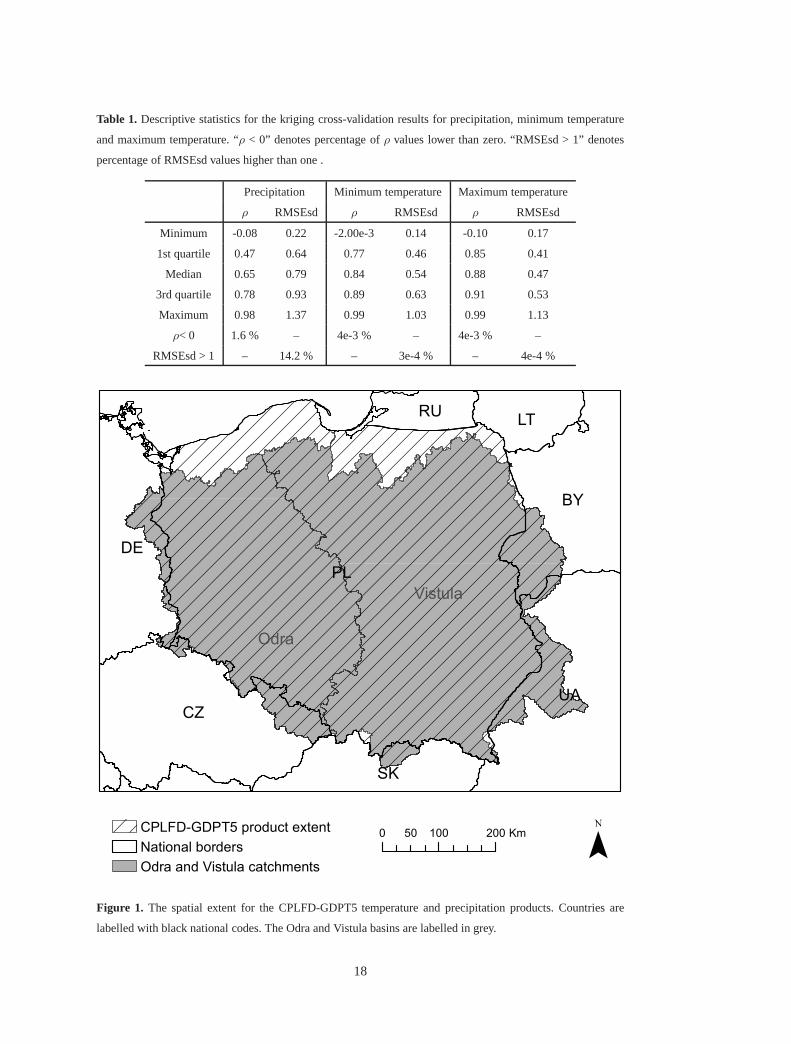
Table 1. Descriptive statistics for the kriging cross-validation results for precipitation, minimum temperature

and maximum temperature. “ρ < 0” denotes percentage ofρ values lower than zero. “RMSEsd > 1” denotes

percentage of RMSEsd values higher than one .

Precipitation Minimum temperature Maximum temperature

ρ RMSEsd ρ RMSEsd ρ RMSEsd

Minimum -0.08 0.22 -2.00e-3 0.14 -0.10 0.17

1st quartile 0.47 0.64 0.77 0.46 0.85 0.41

Median 0.65 0.79 0.84 0.54 0.88 0.47

3rd quartile 0.78 0.93 0.89 0.63 0.91 0.53

Maximum 0.98 1.37 0.99 1.03 0.99 1.13

ρ< 0 1.6 % – 4e-3 % – 4e-3 % –

RMSEsd > 1 – 14.2 % – 3e-4 % – 4e-4 %

PL

CZUA

BY

DE

SK

LTRU

Vistula

Odra

CPLFD-GDPT5 product extent

National borders

Odra and Vistula catchments

0 100 20050 Km

Figure 1. The spatial extent for the CPLFD-GDPT5 temperature and precipitation products. Countries are

labelled with black national codes. The Odra and Vistula basins are labelled in grey.

18

Year

Num

ber

of s

tatio

ns p

er y

ear

0

200

400

600

1960 1980 2000

IMGW−PIBECADNOAADWD

Figure 2. Number of meteorological stations for precipitation observations per year from 1951 to 2013.

Year

Num

ber

of s

tatio

ns p

er y

ear

0

50

100

150

1960 1980 2000

IMGW−PIBECADNOAADWD

Figure 3. Number of meteorological stations for temperature observations per year from 1951 to 2013.

19

Temperature stations

Precipitation stations

CPLFD-GDPT5 product extent

0 100 20050 Km

Figure 4.Spatial distribution of meteorological stations for temperature and precipitation used for interpolation

of the CPLFD-GDPT5 product.

20

PL

CZUA

BY

DE

SK

LTRU

Parameter b for precipitation stations

low shielding

medium shielding

National borders

0 100 20050 Km

Figure 5. The Richter (1995) parameterb value groups for different for precipitation stations.

21

PL

UACZ

BY

DE

SK

LTRU

0 100 20050 Km

Correlation for precipitation stations0.00 - 0.20 0.21 - 0.40 0.41 - 0.60 0.61 - 0.80 0.81 - 1.00

PL

UACZ

BY

DE

SK

LTRU

RMSEsd for precipitation stations0.29 - 0.35 0.36 - 0.70 0.71 - 1.05 1.06 - 1.40 1.41 - 1.75

Figure 6. Precipitationρ (top) and RMSEsd (bottom) values calculated for stations inthe period 1951-2013.

National borders (black lines) are labelled with country codes.

22

Year

1960 1980 2000

0.70

0.75

0.80

0.85

0.90

300

400

500

600

700

Num

ber

of s

tatio

ns p

er y

ear

RM

SE

sd [−

]

Figure 7. Annual RMSEsd median (blue) and number of available stations per year (pink) for precipitation

in the period 1951-2013. The daily results, also summarizedin Table 1, were used for calculating the annual

medians.

23

PL

UACZ

BY

DE

SK

LTRU

0 100 20050 Km

Correlation for minimum temperature stations

0.46 - 0.60 0.61 - 0.80 0.81 - 1.00

PL

UACZ

BY

DE

SK

LTRU

RMSEsd for minimum temperature stations0.06 - 0.20 0.21 - 0.40 0.41 - 0.60 0.61 - 0.80 0.81 - 1.00

Figure 8. Minimum temperatureρ (top) and RMSEsd (bottom) values calculated for stations inthe period

1951-2013. National borders (black lines) are labelled with country codes.

24

PL

UACZ

BY

DE

SK

LTRU

0 100 20050 Km

Correlation for maximum temperature stations0.65 - 0.70 0.71 - 0.80 0.81 - 0.90 0.91 - 1.00

PL

UACZ

BY

DE

SK

LTRU

RMSEsd for maximum temperature stations0.05 - 0.25 0.26 - 0.50 0.51 - 0.75 0.76 - 1.00 1.01 - 1.25

Figure 9. Maximum temperatureρ (top) and RMSEsd (bottom) values calculated for stations inthe period

1951-2013. National borders (black lines) are labelled with country codes.

25

Year

1960 1980 2000

0.50

0.52

0.54

0.56

0.58

0.60

80

100

120

140

160

180

Num

ber

of s

tatio

ns p

er y

ear

RM

SE

sd [−

]

Figure 10. Annual RMSEsd median (blue) and number of available stations per year (pink) for minimum

temperature in the period 1951-2013. The daily results, also summarized in Table 1, were used for calculating

the annual medians.

Year

1960 1980 2000

0.45

0.50

0.55

80

100

120

140

160

180

Num

ber

of s

tatio

ns p

er y

ear

RM

SE

sd [−

]

Figure 11. Annual RMSEsd median (blue) and number of available stations per year (pink) for maximum

temperature in the period 1951-2013. The daily results, also summarized in Table 1, were used for calculating

the annual medians.

26

650

700

75

0 800850

600

650

750 700

650

600

750

700

800

750

650

700

600

13501000

1050

Legend

CPLFD-GDPT5 precipitaion totals contours [mm]IMGW-PIB precipitation totals symbology:

Figure 12. Comparison of CPLFD-GDPT5 precipitation totals contours with IMGW-PIB precipitation totals

map for the 1971-2000 period. Contours are in 50 mm intervals. The IMGW-PIB map indicates also major

rivers (blue lines) and major cities (labelled black circles). The IMGW-PIB map is adapted from the Climatic

Maps of Poland (IMGW-PIB, 2015).

27

-9

-8

-7

-10

-11

-12

-6

-11

-10

-9

-9

-8

-10

-11

-11

-8

-7

-13 -12Legend

CPLFD-GDPT5 5% minimum temperature contours [oC]IMGW-PIB 5% minimum temperature symbology:

Figure 13.Comparison of CPLFD-GDPT5 5% minimum temperatures contours with IMGW-PIB 5% minimum

temperatures map for the 1971-2000 period. Contours are in 1◦C intervals. The IMGW-PIB map indicates also

major rivers (blue lines) and major cities (labelled black circles). The IMGW-PIB map is adapted from the

Climatic Maps of Poland (IMGW-PIB, 2015).

28

26

27

25

24

26

27

26

26

27

27

27

25

26

2425

27

27

27

26

24

25

27

26

25

24

27

27

27

26

26

25

27

25

26

26

27

27

27

27

25

26

27

18 23Legend

CPLFD-GDPT5 95% maximum temperature contours [oC]IMGW-PIB 95% maximum temperature symbology:

Figure 14.Comparison of CPLFD-GDPT5 95% maximum temperatures contours with IMGW-PIB 95% maxi-

mum temperatures map for the 1971-2000 period. Contours arein 1◦C intervals. The IMGW-PIB map indicates

also major rivers (blue lines) and major cities (labelled black circles). The IMGW-PIB map is adapted from the

Climatic Maps of Poland (IMGW-PIB, 2015).

29

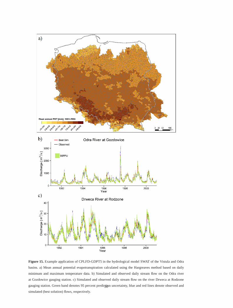
Figure 15. Example application of CPLFD-GDPT5 in the hydrological model SWAT of the Vistula and Odra

basins. a) Mean annual potential evapotranspiration calculated using the Hargreaves method based on daily

minimum and maximum temperature data. b) Simulated and observed daily stream flow on the Odra river

at Gozdowice gauging station. c) Simulated and observed daily stream flow on the river Drweca at Rodzone

gauging station. Green band denotes 95 percent prediction uncertainty, blue and red lines denote observed and

simulated (best solution) flows, respectively.

30