Copyright crab.ict.pwr.wroc.pl/~kreczmer/wds/MATERIALY/gnuplot1.pdf · Najprostszy wykres plot...
30
Wprowadzenie do programu gnuplot Bogdan Kreczmer ZPCiR ICT PWR pokój 307 budynek C3 [email protected] Copyright c 2003 Bogdan Kreczmer Niniejszy dokument zawiera materialy do wykladu na temat wizualizacji danych sensorycznych. Jest on udost ˛ epiony pod warunkiem wykorzystania wyl ˛ acznie do wlasnych prywatnych potrzeb i mo˙ ze on by ´ c kopiowany wyl ˛ acznie w calo ´ sci, razem z ninijesz ˛ a stron ˛ a tytulow ˛ a. – Sklad Foil T E X–
Transcript of Copyright crab.ict.pwr.wroc.pl/~kreczmer/wds/MATERIALY/gnuplot1.pdf · Najprostszy wykres plot...

Wprowadzenie do programu gnuplot
Bogdan KreczmerZPCiR ICT PWR
pokój 307 budynek C3
Copyright c� 2003 Bogdan Kreczmer �
� Niniejszy dokument zawiera materiały do wykładu na temat wizualizacji danych sensorycznych. Jest on udostepionypod warunkiem wykorzystania wyłacznie do własnych prywatnych potrzeb i moze on byc kopiowany wyłacznie w całosci,razem z ninijesza strona tytułowa.
– Skład FoilTEX–

gnuplot
Główni autorzy: Thomas Williams, Colin Kelley
http://www.gnuplot.info/ftp://ftp.gnuplot.info/pub/gnuplot/
gnuplot jest programem przeznaczonym do:
� tworzenia rysunków wykresów funkcji jedno i dwuargumentowych (funkcje moga bycparametryzowane),
� obrazowania danych pomiarowych,
� tworzenia wykresów interpolujacych przebiegi funkcji na podstawie zbioru danychpomiarowych. Przy interpolacji brane sa pod uwage błedy zwiazane z zadanymiwartosciami.
Jest to program zorientowany na polecenia tekstowe w pracy interaktywnej lub wsado-wej.
gnuplot 1
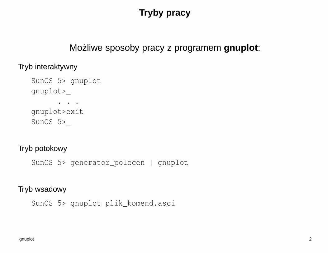
Tryby pracy
Mozliwe sposoby pracy z programem gnuplot:
Tryb interaktywny
SunOS 5> gnuplotgnuplot>_
. . .gnuplot>exitSunOS 5>_
Tryb potokowy
SunOS 5> generator_polecen | gnuplot
Tryb wsadowy
SunOS 5> gnuplot plik_komend.asci
gnuplot 2

Podpowiedzi - help
gnuplot> help‘gnuplot‘ is a command-driven interactive function and data plotting program.It is case sensitive (commands and function names written in lowercase arenot the same as those written in CAPS). All command names may be abbreviatedas long as the abbreviation is not ambiguous. Any number of commands may
. . .
Help topics available:batch/interactive bugs commands commentscoordinates copyright environment expressionsglossary graphical introduction line-editingnew-features old_bugs plotting seeking-assistanceset show startup substitutionsyntax time/date
Help topic: _
gnuplot 3
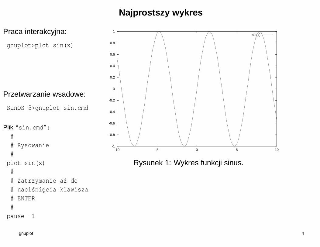
Najprostszy wykres
Praca interakcyjna:
gnuplot>plot sin(x)
Przetwarzanie wsadowe:
SunOS 5>gnuplot sin.cmd
Plik “sin.cmd”:## Rysowanie#plot sin(x)## Zatrzymanie az do# nacisniecia klawisza# ENTER#pause -1
-1
-0.8
-0.6
-0.4
-0.2
0
0.2
0.4
0.6
0.8
1
-10 -5 0 5 10
sin(x)
Rysunek 1: Wykres funkcji sinus.
gnuplot 4

Najprostszy wykres
plot sin(x) with lines 2
plot sin(x) w l 2
Składnia sekcji withdla polecenia plot:
with <style> { {linestyle | ls <line_style>}| {{linetype | lt <line_type>} {linewidth | lw <line_width>}
{pointtype | pt <point_type>} {pointsize | ps <point_size>}} }
-1
-0.8
-0.6
-0.4
-0.2
0
0.2
0.4
0.6
0.8
1
-10 -5 0 5 10
sin(x)
<style> = lines | points | linespoints | impulses | dots | steps | fsteps |histeps | errorbars | xerrorbars | yerrorbars | xyerrorbars |boxes | xyerrorbars | boxes | boxerrorbars | boxxyerrorbars |financebars | candlesticks | candlesticks | vector
gnuplot 5
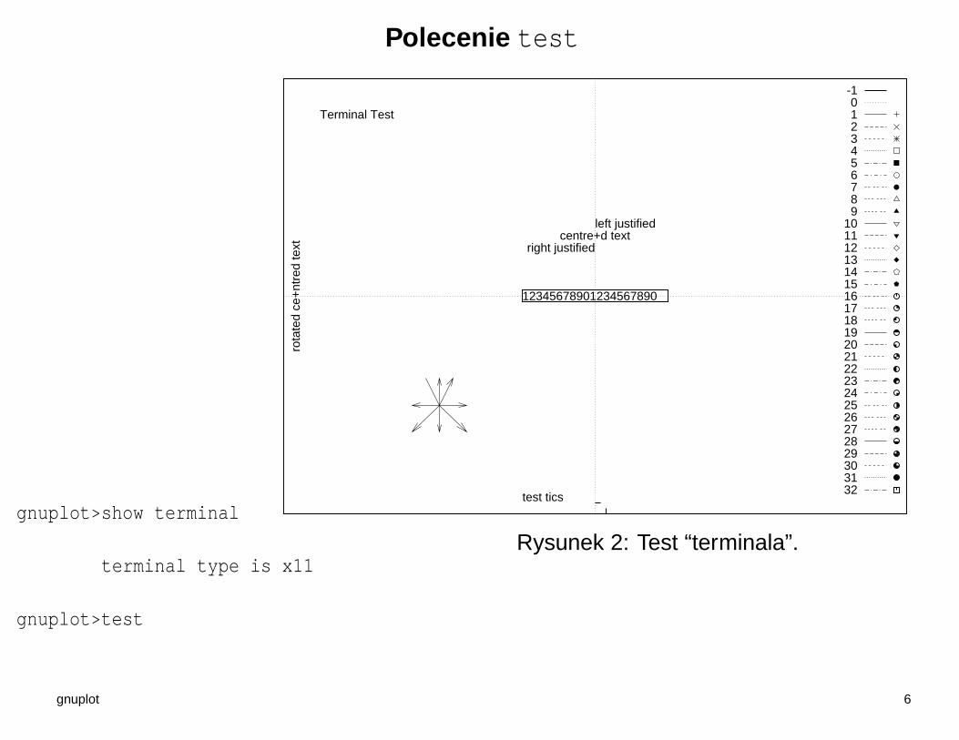
Polecenie test
gnuplot>show terminal
terminal type is x11
gnuplot>test
Terminal Test
12345678901234567890
left justifiedcentre+d text
right justified
rota
ted
ce+
ntre
d te
xt
test tics
-10123456789
1011121314151617181920212223242526272829303132
Rysunek 2: Test “terminala”.
gnuplot 6

Przykłady stylów rysowania
-1
-0.8
-0.6
-0.4
-0.2
0
0.2
0.4
0.6
0.8
1
-10 -5 0 5 10
sin(x)
-1
-0.8
-0.6
-0.4
-0.2
0
0.2
0.4
0.6
0.8
1
-10 -5 0 5 10
sin(x)
-1
-0.8
-0.6
-0.4
-0.2
0
0.2
0.4
0.6
0.8
1
-10 -5 0 5 10
sin(x)
plot sin(x) with l lt 2 plot sin(x) with l lt 3 lw 3 plot sin(x) with l lt 7 lw 9
-1
-0.8
-0.6
-0.4
-0.2
0
0.2
0.4
0.6
0.8
1
-10 -5 0 5 10
sin(x)
-1
-0.8
-0.6
-0.4
-0.2
0
0.2
0.4
0.6
0.8
1
-10 -5 0 5 10
sin(x)
-1
-0.8
-0.6
-0.4
-0.2
0
0.2
0.4
0.6
0.8
1
-10 -5 0 5 10
sin(x)
plot sin(x) with points plot sin(x) with points pt 1 ps 4 plot sin(x) with p lt 2 pt 2 ps 8
-1
-0.8
-0.6
-0.4
-0.2
0
0.2
0.4
0.6
0.8
1
-10 -5 0 5 10
sin(x)
-1
-0.8
-0.6
-0.4
-0.2
0
0.2
0.4
0.6
0.8
1
-10 -5 0 5 10
sin(x)
-1
-0.8
-0.6
-0.4
-0.2
0
0.2
0.4
0.6
0.8
1
-10 -5 0 5 10
sin(x)
plot sin(x) with linespoints lt 2 ... w linesp lt 3 lw 3 pt 1 ps 4 ... w linesp lt 7 lw 9 pt 2 ps 8gnuplot 7
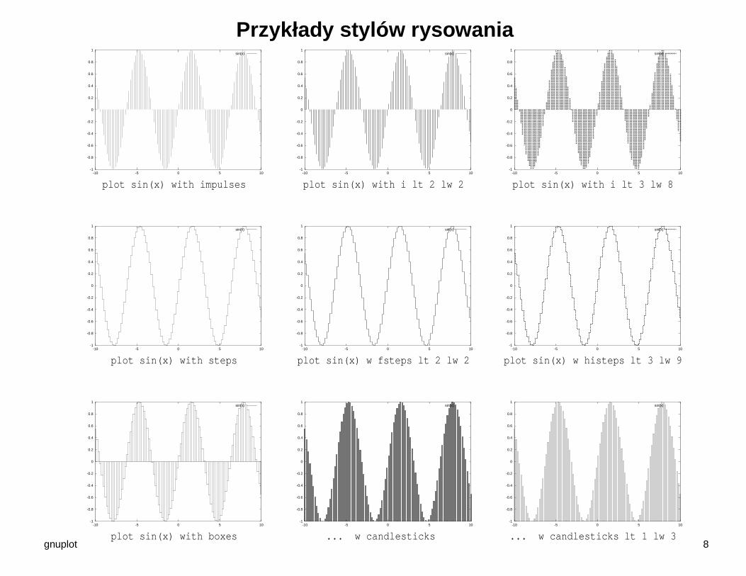
Przykłady stylów rysowania
-1
-0.8
-0.6
-0.4
-0.2
0
0.2
0.4
0.6
0.8
1
-10 -5 0 5 10
sin(x)
-1
-0.8
-0.6
-0.4
-0.2
0
0.2
0.4
0.6
0.8
1
-10 -5 0 5 10
sin(x)
-1
-0.8
-0.6
-0.4
-0.2
0
0.2
0.4
0.6
0.8
1
-10 -5 0 5 10
sin(x)
plot sin(x) with impulses plot sin(x) with i lt 2 lw 2 plot sin(x) with i lt 3 lw 8
-1
-0.8
-0.6
-0.4
-0.2
0
0.2
0.4
0.6
0.8
1
-10 -5 0 5 10
sin(x)
-1
-0.8
-0.6
-0.4
-0.2
0
0.2
0.4
0.6
0.8
1
-10 -5 0 5 10
sin(x)
-1
-0.8
-0.6
-0.4
-0.2
0
0.2
0.4
0.6
0.8
1
-10 -5 0 5 10
sin(x)
plot sin(x) with steps plot sin(x) w fsteps lt 2 lw 2 plot sin(x) w histeps lt 3 lw 9
-1
-0.8
-0.6
-0.4
-0.2
0
0.2
0.4
0.6
0.8
1
-10 -5 0 5 10
sin(x)
-1
-0.8
-0.6
-0.4
-0.2
0
0.2
0.4
0.6
0.8
1
-10 -5 0 5 10
sin(x)
-1
-0.8
-0.6
-0.4
-0.2
0
0.2
0.4
0.6
0.8
1
-10 -5 0 5 10
sin(x)
plot sin(x) with boxes ... w candlesticks ... w candlesticks lt 1 lw 3gnuplot 8
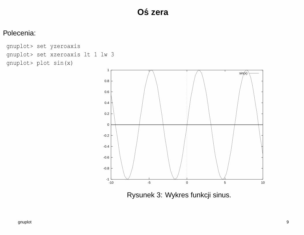
Os zera
Polecenia:
gnuplot> set yzeroaxisgnuplot> set xzeroaxis lt 1 lw 3gnuplot> plot sin(x)
-1
-0.8
-0.6
-0.4
-0.2
0
0.2
0.4
0.6
0.8
1
-10 -5 0 5 10
sin(x)
Rysunek 3: Wykres funkcji sinus.
gnuplot 9

Z radianów na stopnie
Polecenia:
gnuplot> set angles degreesgnuplot> plot [0:360] sin(x)
-1
-0.8
-0.6
-0.4
-0.2
0
0.2
0.4
0.6
0.8
1
0 50 100 150 200 250 300 350
sin(x)
Rysunek 4: Wykres funkcji sinus.
gnuplot 10
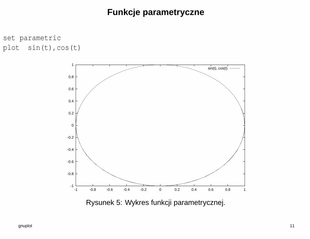
Funkcje parametryczne
set parametricplot sin(t),cos(t)
-1
-0.8
-0.6
-0.4
-0.2
0
0.2
0.4
0.6
0.8
1
-1 -0.8 -0.6 -0.4 -0.2 0 0.2 0.4 0.6 0.8 1
sin(t), cos(t)
Rysunek 5: Wykres funkcji parametrycznej.
gnuplot 11

Wzajemna proporcjonalnosc osi
gnuplot> . . .gnuplot> set size ratio 1gnuplot> set parametricgnuplot> plot sin(t),cos(t)
noratio ratio: 1 ratio: 1.33
-2
-1.5
-1
-0.5
0
0.5
1
1.5
2
-1.5 -1 -0.5 0 0.5 1 1.5
sin(t), cos(t)
-2
-1.5
-1
-0.5
0
0.5
1
1.5
2
-2 -1.5 -1 -0.5 0 0.5 1 1.5 2
sin(t), cos(t)
-2
-1.5
-1
-0.5
0
0.5
1
1.5
2
-1.5 -1 -0.5 0 0.5 1 1.5
sin(t), cos(t)
set size {{no}square | ratio <r> | noratio} {<xscale>,<yscale>}
gnuplot 12
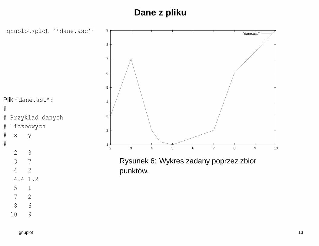
Dane z pliku
gnuplot>plot ’’dane.asc’’
Plik ”dane.asc”:## Przyklad danych# liczbowych# x y#
2 33 74 24.4 1.25 17 28 610 9
1
2
3
4
5
6
7
8
9
2 3 4 5 6 7 8 9 10
"dane.asc"
Rysunek 6: Wykres zadany poprzez zbiorpunktów.
gnuplot 13
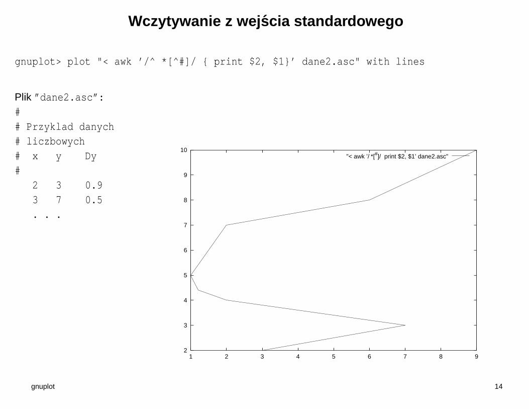
Wczytywanie z wejscia standardowego
gnuplot> plot "< awk ’/^ *[^#]/ { print $2, $1}’ dane2.asc" with lines
Plik ”dane2.asc”:## Przyklad danych# liczbowych# x y Dy#
2 3 0.93 7 0.5. . .
2
3
4
5
6
7
8
9
10
1 2 3 4 5 6 7 8 9
"< awk ’/ *[#]/ print $2, $1’ dane2.asc"
gnuplot 14
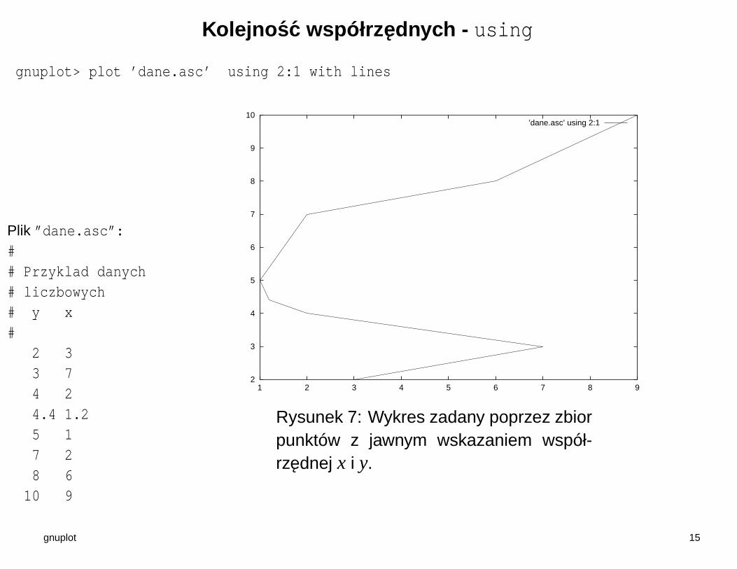
Kolejnosc współrzednych - using
gnuplot> plot ’dane.asc’ using 2:1 with lines
Plik ”dane.asc”:## Przyklad danych# liczbowych# y x#
2 33 74 24.4 1.25 17 28 610 9
2
3
4
5
6
7
8
9
10
1 2 3 4 5 6 7 8 9
’dane.asc’ using 2:1
Rysunek 7: Wykres zadany poprzez zbiorpunktów z jawnym wskazaniem współ-rzednej x i y.
gnuplot 15
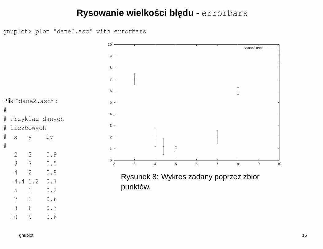
Rysowanie wielkosci błedu - errorbars
gnuplot> plot "dane2.asc" with errorbars
Plik ”dane2.asc”:## Przyklad danych# liczbowych# x y Dy#
2 3 0.93 7 0.54 2 0.84.4 1.2 0.75 1 0.27 2 0.68 6 0.310 9 0.6
0
1
2
3
4
5
6
7
8
9
10
2 3 4 5 6 7 8 9 10
"dane2.asc"
Rysunek 8: Wykres zadany poprzez zbiorpunktów.
gnuplot 16
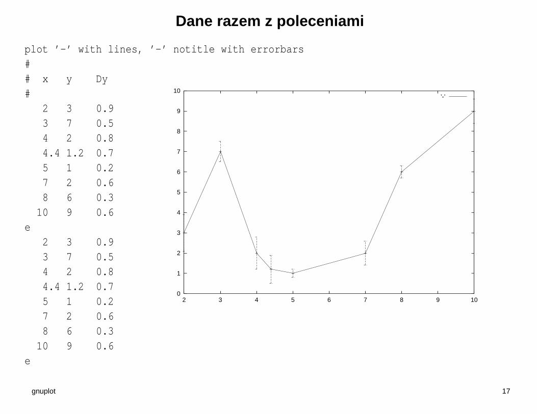
Dane razem z poleceniami
plot ’-’ with lines, ’-’ notitle with errorbars## x y Dy#
2 3 0.93 7 0.54 2 0.84.4 1.2 0.75 1 0.27 2 0.68 6 0.310 9 0.6
e2 3 0.93 7 0.54 2 0.84.4 1.2 0.75 1 0.27 2 0.68 6 0.310 9 0.6
e
0
1
2
3
4
5
6
7
8
9
10
2 3 4 5 6 7 8 9 10
’-’
gnuplot 17
Rysowanie wielkosci błedu - errorbars
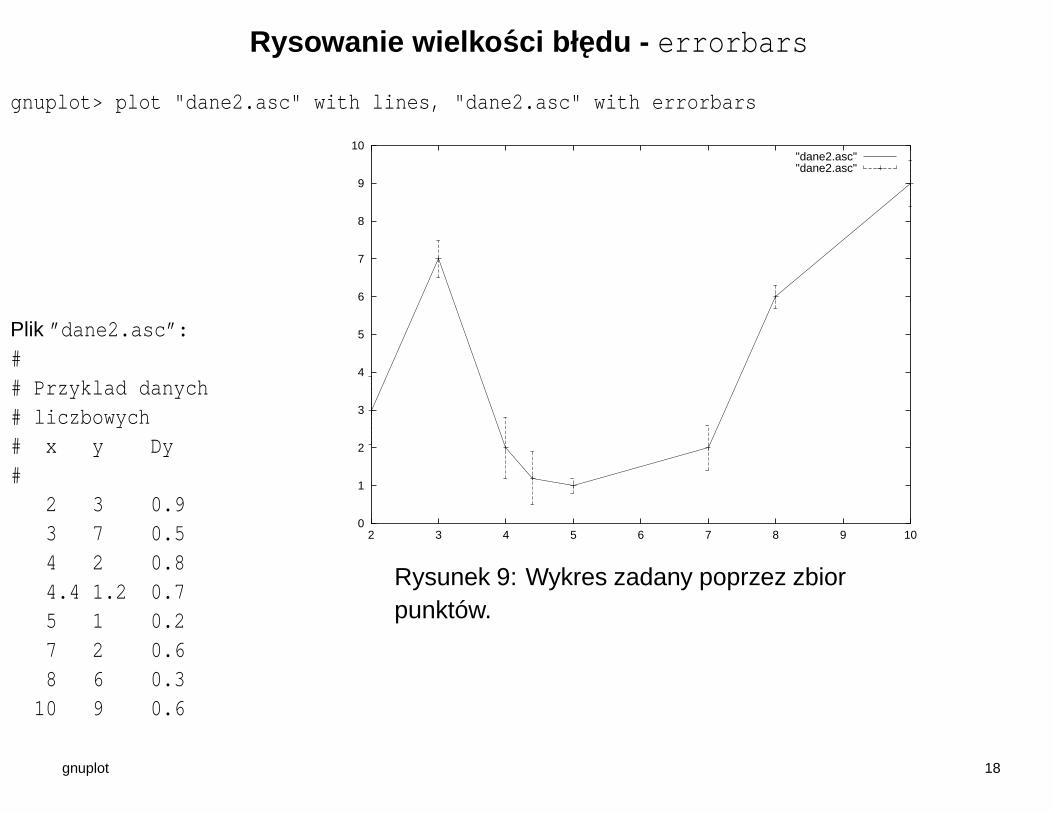
gnuplot> plot "dane2.asc" with lines, "dane2.asc" with errorbars
Plik ”dane2.asc”:## Przyklad danych# liczbowych# x y Dy#
2 3 0.93 7 0.54 2 0.84.4 1.2 0.75 1 0.27 2 0.68 6 0.310 9 0.6
0
1
2
3
4
5
6
7
8
9
10
2 3 4 5 6 7 8 9 10
"dane2.asc""dane2.asc"
Rysunek 9: Wykres zadany poprzez zbiorpunktów.
gnuplot 18

Rysowanie wielkosci błedu - xyerrorbars
gnuplot> plot "dane3.asc" with xyerrorbars
Plik ”dane3.asc”:## Przyklad danych# liczbowych# x y Dx Dy#
2 3 0.5 0.93 7 0.2 0.54 2 0.9 0.84.4 1.2 0.4 0.75 1 0.6 0.27 2 0.8 0.68 6 0.4 0.310 9 0.4 0.6
0
1
2
3
4
5
6
7
8
9
10
1 2 3 4 5 6 7 8 9 10 11
"dane3.asc"
Rysunek 10: Wykres zadany poprzezzbior punktów z informacja o błedach.
gnuplot 19

Rysowanie z wygładzaniem
gnuplot> plot "dane.asc" smooth csplines
Plik ”dane.asc”:## Przyklad danych# liczbowych# x y#
2 33 74 24.4 1.25 17 28 610 9
0
1
2
3
4
5
6
7
8
9
2 3 4 5 6 7 8 9 10
’dane.asc’
Rysunek 11: Wykres zadany poprzezzbior punktów. Rysunek z wygładzaniem.
gnuplot 20
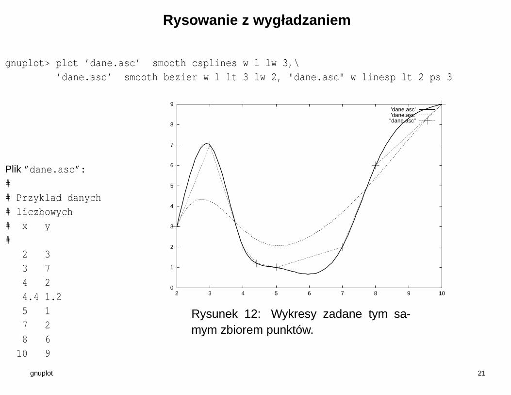
Rysowanie z wygładzaniem
gnuplot> plot ’dane.asc’ smooth csplines w l lw 3,\’dane.asc’ smooth bezier w l lt 3 lw 2, "dane.asc" w linesp lt 2 ps 3
Plik ”dane.asc”:## Przyklad danych# liczbowych# x y#
2 33 74 24.4 1.25 17 28 610 9
0
1
2
3
4
5
6
7
8
9
2 3 4 5 6 7 8 9 10
’dane.asc’’dane.asc’"dane.asc"
Rysunek 12: Wykresy zadane tym sa-mym zbiorem punktów.
gnuplot 21
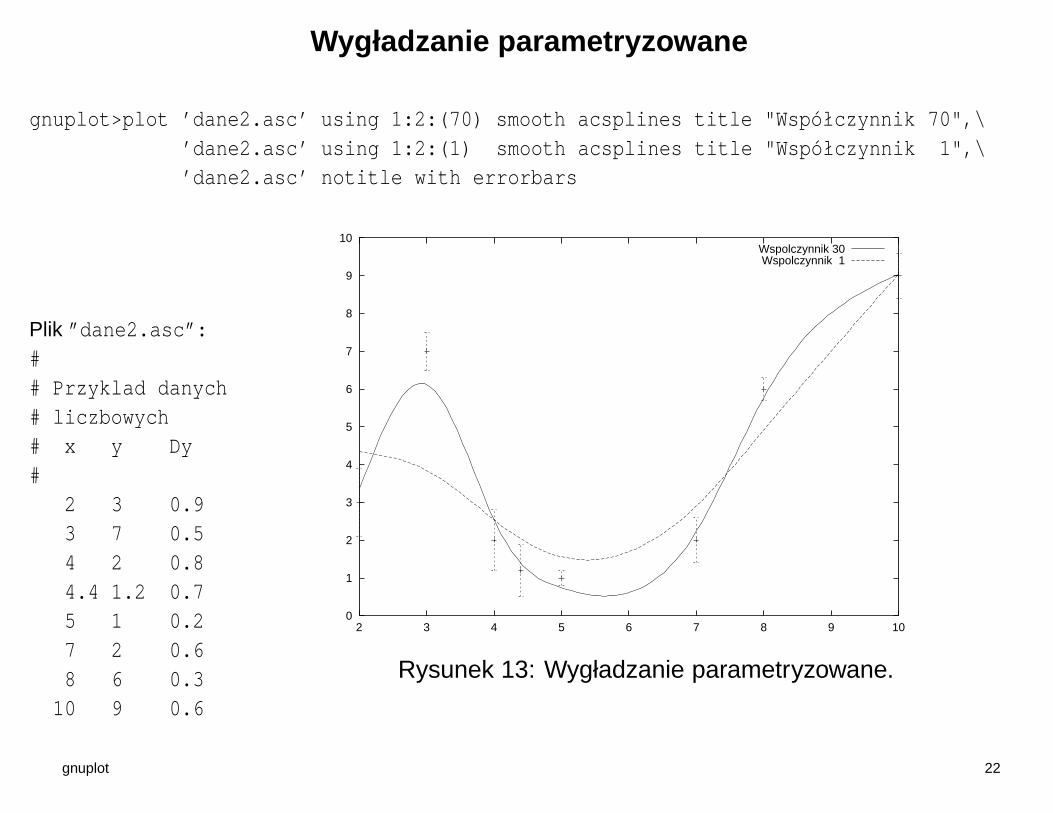
Wygładzanie parametryzowane
gnuplot>plot ’dane2.asc’ using 1:2:(70) smooth acsplines title "Współczynnik 70",\’dane2.asc’ using 1:2:(1) smooth acsplines title "Współczynnik 1",\’dane2.asc’ notitle with errorbars
Plik ”dane2.asc”:## Przyklad danych# liczbowych# x y Dy#
2 3 0.93 7 0.54 2 0.84.4 1.2 0.75 1 0.27 2 0.68 6 0.310 9 0.6
0
1
2
3
4
5
6
7
8
9
10
2 3 4 5 6 7 8 9 10
Wspolczynnik 30Wspolczynnik 1
Rysunek 13: Wygładzanie parametryzowane.
gnuplot 22
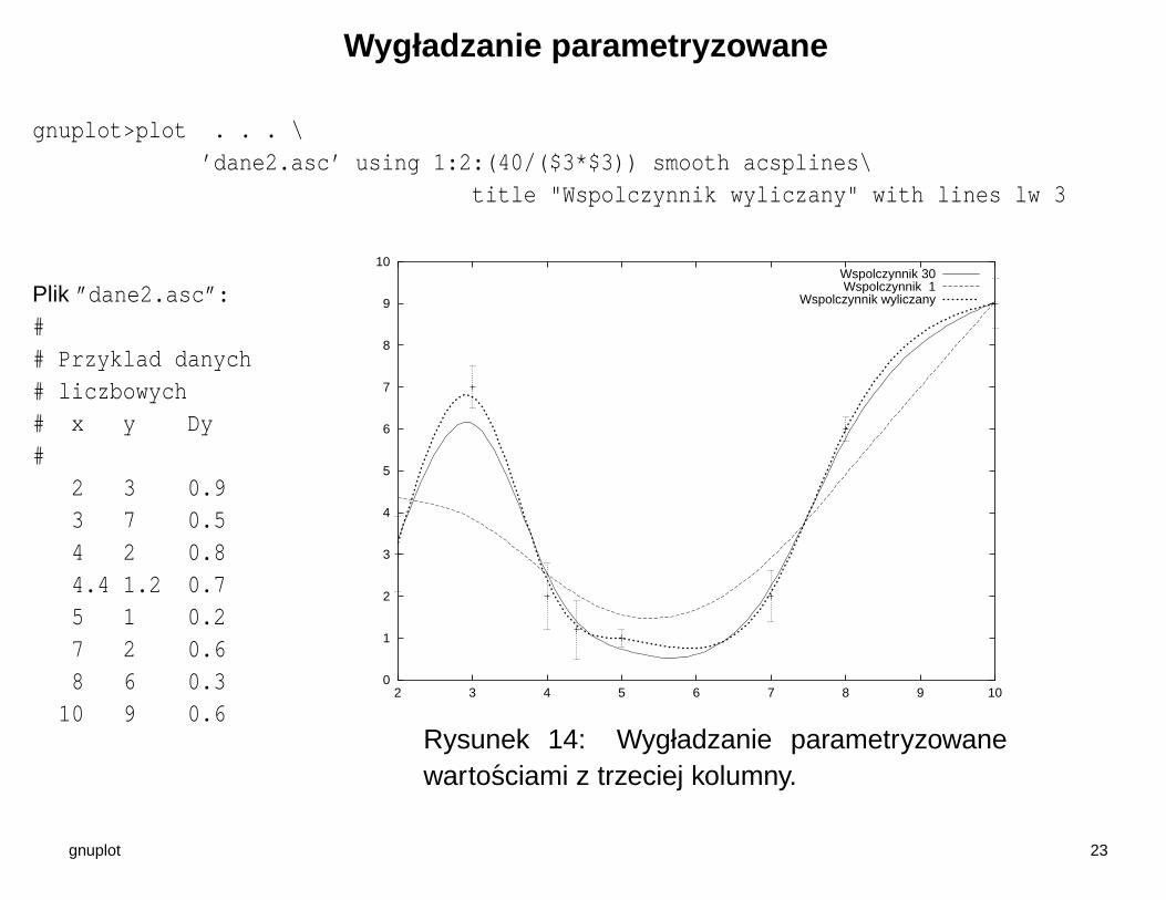
Wygładzanie parametryzowane
gnuplot>plot . . . \’dane2.asc’ using 1:2:(40/($3*$3)) smooth acsplines\
title "Wspolczynnik wyliczany" with lines lw 3
Plik ”dane2.asc”:## Przyklad danych# liczbowych# x y Dy#
2 3 0.93 7 0.54 2 0.84.4 1.2 0.75 1 0.27 2 0.68 6 0.310 9 0.6
0
1
2
3
4
5
6
7
8
9
10
2 3 4 5 6 7 8 9 10
Wspolczynnik 30Wspolczynnik 1
Wspolczynnik wyliczany
Rysunek 14: Wygładzanie parametryzowanewartosciami z trzeciej kolumny.
gnuplot 23

Zakres - range
gnuplot> plot [1:11] [0:10] ’dane.asc’ with lines
## Drugi sposób:#
set xrange [1:11]set yrange [0:10]plot ’dane.asc’ w lines
0
2
4
6
8
10
2 4 6 8 10
’dane.asc’
Rysunek 15: Wykres zadany poprzezzbior punktów z własnym ustawieniem za-kresu zmian współrzednych.
gnuplot 24
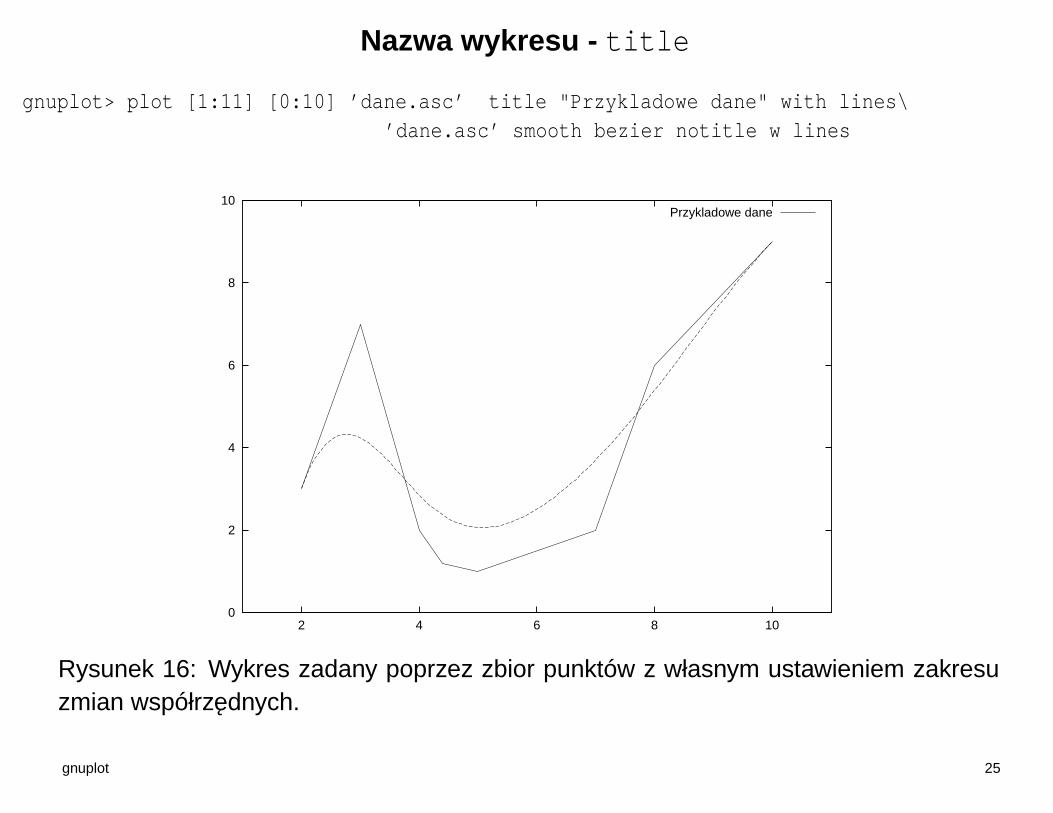
Nazwa wykresu - title
gnuplot> plot [1:11] [0:10] ’dane.asc’ title "Przykladowe dane" with lines\’dane.asc’ smooth bezier notitle w lines
0
2
4
6
8
10
2 4 6 8 10
Przykladowe dane
Rysunek 16: Wykres zadany poprzez zbior punktów z własnym ustawieniem zakresuzmian współrzednych.
gnuplot 25
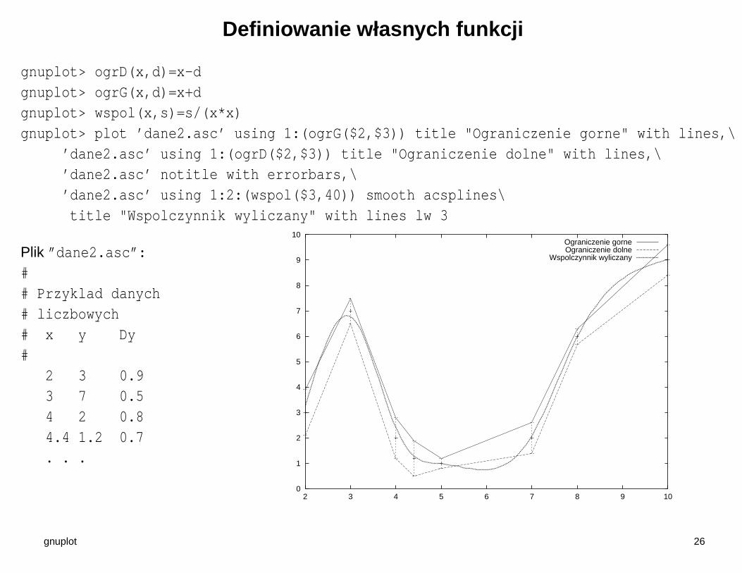
Definiowanie własnych funkcji
gnuplot> ogrD(x,d)=x-dgnuplot> ogrG(x,d)=x+dgnuplot> wspol(x,s)=s/(x*x)gnuplot> plot ’dane2.asc’ using 1:(ogrG($2,$3)) title "Ograniczenie gorne" with lines,\
’dane2.asc’ using 1:(ogrD($2,$3)) title "Ograniczenie dolne" with lines,\’dane2.asc’ notitle with errorbars,\’dane2.asc’ using 1:2:(wspol($3,40)) smooth acsplines\title "Wspolczynnik wyliczany" with lines lw 3
Plik ”dane2.asc”:## Przyklad danych# liczbowych# x y Dy#
2 3 0.93 7 0.54 2 0.84.4 1.2 0.7. . .
0
1
2
3
4
5
6
7
8
9
10
2 3 4 5 6 7 8 9 10
Ograniczenie gorneOgraniczenie dolne
Wspolczynnik wyliczany
gnuplot 26
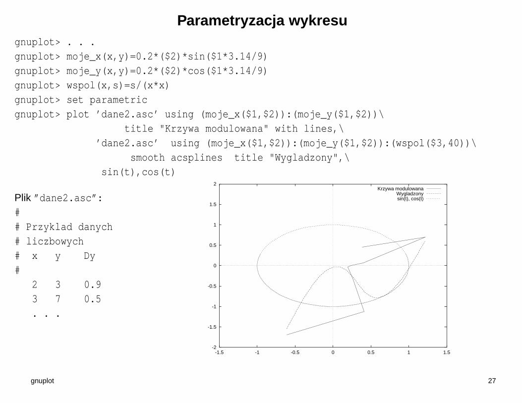
Parametryzacja wykresugnuplot> . . .gnuplot> moje_x(x,y)=0.2*($2)*sin($1*3.14/9)gnuplot> moje_y(x,y)=0.2*($2)*cos($1*3.14/9)gnuplot> wspol(x,s)=s/(x*x)gnuplot> set parametricgnuplot> plot ’dane2.asc’ using (moje_x($1,$2)):(moje_y($1,$2))\
title "Krzywa modulowana" with lines,\’dane2.asc’ using (moje_x($1,$2)):(moje_y($1,$2)):(wspol($3,40))\
smooth acsplines title "Wygladzony",\sin(t),cos(t)
Plik ”dane2.asc”:## Przyklad danych# liczbowych# x y Dy#
2 3 0.93 7 0.5. . .
-2
-1.5
-1
-0.5
0
0.5
1
1.5
2
-1.5 -1 -0.5 0 0.5 1 1.5
Krzywa modulowanaWygladzonysin(t), cos(t)
gnuplot 27
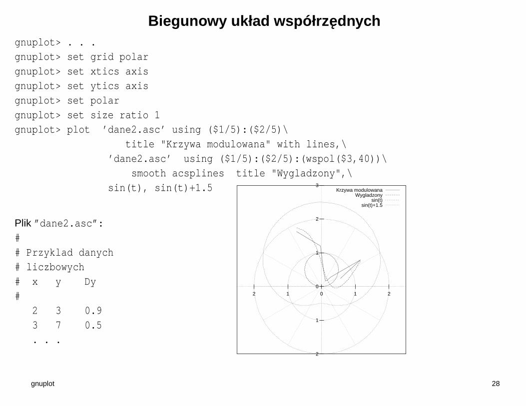
Biegunowy układ współrzednychgnuplot> . . .gnuplot> set grid polargnuplot> set xtics axisgnuplot> set ytics axisgnuplot> set polargnuplot> set size ratio 1gnuplot> plot ’dane2.asc’ using ($1/5):($2/5)\
title "Krzywa modulowana" with lines,\’dane2.asc’ using ($1/5):($2/5):(wspol($3,40))\
smooth acsplines title "Wygladzony",\sin(t), sin(t)+1.5
Plik ”dane2.asc”:## Przyklad danych# liczbowych# x y Dy#
2 3 0.93 7 0.5. . .
2
1
0
1
2
3
2 1 0 1 2
Krzywa modulowanaWygladzony
sin(t)sin(t)+1.5
gnuplot 28

Siatka i podziałka
gnuplot> set y2ticsgnuplot> set my2tics 2gnuplot> set mxticsgnuplot> set gridgnuplot> plot ’dane2.asc’ with lines
set grid set grid xtics set grid xtics ytics mytics
1
2
3
4
5
6
7
8
9
2 3 4 5 6 7 8 9 101
2
3
4
5
6
7
8
9’dane2.asc’
1
2
3
4
5
6
7
8
9
2 3 4 5 6 7 8 9 101
2
3
4
5
6
7
8
9’dane2.asc’
1
2
3
4
5
6
7
8
9
2 3 4 5 6 7 8 9 101
2
3
4
5
6
7
8
9’dane2.asc’
set grid {{no}{m}xtics} {{no}{m}ytics} {{no}{m}ztics}{{no}{m}x2tics} {{no}{m}y2tics}{polar {<angle>}} { {linestyle <major_linestyle>}
| {linetype | lt <major_linetype>} ...
gnuplot 29