
Acta Energetica Power Engineering Quarterly no. 01/2009
120
01/2009 number 1/year 1 nergetica act Electrical Power Engineering Quarterly
description
Acta Energetica is a scientific journal devoted to power engineering. It is published by the Polish energy holding Energa SA under the patronage of Gdańsk University of Technology.
Transcript of Acta Energetica Power Engineering Quarterly no. 01/2009

01/2009 number 1/year 1
nergeticaact Electrical Power Engineering Quarterly

www. actaenergetica.org

Publisher
Patronage
Gdańsk University of Technology
ENERGA S.A.
Editor-in-ChiefZbigniew Lubośny
Academic ConsultantsJanusz Białek / Mieczysław Brdyś / Antoni Dmowski / Istvan Erlich / Andrzej GraczykTadeusz Kaczorek / Marian Kaźmierkowski / Jan Kiciński / Jerzy KulczyckiKwang Y. Lee / Zbigniew Lubośny / Jan Machowski / Om Malik / Jovica MilanovicJan Popczyk / Zbigniew Szczerba / G. Kumar Venayagamoorthy / Jacek Wańkowicz
Editorial Staff OfficeActa Energeticaul. Grodzka 12, 80-841 Gdańsk, POLANDtel.: +48 58 320 00 94, fax: +48 58 320 00 90e-mail: [email protected]. actaenergetica.org
Graphic designMirosław Miłogrodzki
TranslationMaria StelmasiewiczWitold Zbirohowski-Kościa
ProofreadingMirosław Wójcik
Editorial SupportKatarzyna Żelazek
ISSN 2080-7570
Content
INNOVATIVE POWER INDUSTRY. ECOLOGICAL-POWER ENGINEERING AND ECONOMIC -CIVILISATION CONTEXTJan Popczyk
CURRENT DISTORTION IN LIGHTING SYSTEMS AND ITS IMPACT ON POWER SUPPLY INSTALLATIONSStanisław Czapp
DEVELOPMENT OF CO2 EMISSION TRADING IN THE EUROPEAN UNIONAndrzej Graczyk
CONDITIONS FAVOURING VOLTAGE AVALANCHE IN THE OPERATION OF GENERATOR REGULATORS – SELECTED ISSUESJacek Klucznik / Robert Małkowski / Piotr Szczeciński / Ryszard Zajczyk
POWER LOSSES AS NECESSARY OWN NEEDS OF NETWORKJerzy Kulczycki / Michał RudzińskiWaldemar Szpyra
ANALYTICAL DERIVATION OF PSS PARAMETERSFOR GENERATOR WITH STATIC EXCITATION SYSTEMZbigniew Lubośny / Janusz W. Białek
PPN - LIVE CONDUCTOR OPERATIONS ON 400 KV, 220 KV AND 110 KV OVERHEAD TRANSMISSION AND DISTRIBUTION LINES IN ENERGA-OPERATOR S.A. TORUŃ BRANCH.Ryszard Michniewski
MEASUREMENT OF PARTIAL DISCHARGES IN MEDIUM VOLTAGE CABLE LINESSławomir Noske
nergeticaact
8
24
40
48
58
78
94
104
Electrical Power Engineering Quarterly

Gdańsk University of Technology is the oldest and the largest technical college in the North of Poland. Its origins go back to the autumn of 1904, when the Royal Technical College (Königliche Technische Hochs-chule) was founded. It was the first academic school in Gdańsk. Its goal was to spread technical knowledge in the West Prussia and Pomeranian area. From the very beginning the school was located in the beautiful buildings designed by Albert Carsten, built between 1900 and 1904 and well preserved until today.
The college was to educate 600 students in the first years of its operation. All in all, about sixteen thousand students were matriculated until 1945. After World War II, on May 24, 1945 Gdańsk University of Technology, the first Polish state college was founded by virtue of the decree of State National Council. The citizens started renovation of the premises ruined and burnt during the War already in April 1945. The teachers, including many distinguished professors, came mainly from Lvov, Vilnius and Warsaw.
At present Gdańsk University of Technology has 9 faculties, 7 of which have full academic rights. About 24 000 students are studying at 27 specialisations, 3 of which are interdepartmental and 1 - intercol-legiate. Gdańsk University of Technology provides education on engineer, master and doctoral levels in all fields of science, starting from civil engineering and architecture, our oldest specialisations, to modern elec-tronic engineering, material nanotechnology, biotechnology or biomedical engineering. Economics, busi-ness administration and social sciences seem to naturally complete the studies in technical fields.
Our school confirms its well established reputation of a strong educational, scientific and cultural centre by cooperating with other universities and research institutions in Poland and abroad. We cooperate with many companies, educational and cultural organisations and state agencies in the ambition to create a good image of Gdańsk, Pomerania, Poland and Europe.
Cooperation between Gdańsk University of Technology and the region’s business community is get-ting stricter and stronger every year. We are closely related particularly to the Pomeranian Chamber of Commerce and to science and technology parks. Our goal is to stimulate cooperation so that the scientific community’s achievements could be effectively applied in economy. Each year the college very actively participates in the “Industrial Technology, Science and Innovation Fair” held in the Gdańsk International Fair Co., where we present innovative solutions and their applications in the economic environment. We also win many medals and awards.
It is the graduates of Gdańsk University of Technology that create the school’s unique character and reputation. They manage industries and take part in the formation of our country’s present and future. They conduct research in science centres and create new 21st century technologies. We have all the reasons to claim that Gdańsk University of Technology’s diploma can pave the way to professional success and to re-alisation of one’s aspirations.
Let us achieve our basic goals with imagination and wisdom. Therefore, I ask you all to take up new challenges, indispensable for further development of our college in the age of constantly changing environment and global competition. Cooperation between Gdańsk University of Technology and ENERGA Energetic Concern in the field of power industry is one of such challenges. The newly-founded scientific and technical magazine Acta Energetica constitutes a synergic result of our cooperation.
May the authors of this magazine enjoy its every success and the readers - a pleasant and instructive reading.
Prof. Henryk Krawczyk Rector of GUT

The European power industry is undergoing an enormous transformation. There are two goals: to increase power supply security and at the same time to reduce the environmental impact. These priorities express our care about the present as well as about the future. It will be difficult to make them a reality because it requires from the power industry companies to get involved in projects which some stockhold-ers might consider controversial. Our cooperation with the science community shall support this kind of involvement. That is why ENERGA Group together with Gdańsk University of Technology has founded Acta Energetica magazine. Its first issue is right in your hands.
Innovativeness is the key concept for the development of such a company as ENERGA. We consider this notion in a far broader way than only being ready to buy new technologies. We want to participate in their creation. We also want to explain the consequences of formal regulations and postulate their change for the benefit of our customers. By stimulating development of certain areas of power industry we wish Acta Energetica to support popularization, both in Poland and abroad, of the research carried out by the scientists, particularly at the Gdańsk University of Technology. We would like this magazine to contribute to faster implementation of new technical and technological solutions in ENERGA Group. The technical ideas of both institutions should become visible in various scientific and economic environments.
That is why I encourage you to read Acta Energetica.
Mirosław BielińskiPresident of the Board of ENERGA S.A.

WHAT ARE OUR OBJECTIVES?
The challenges of contemporary electrical power systems are the challenges of Acta Energetica
Controlling power engineering subsystems highly saturated with dispersed sources, i.e. intelligent systems• Development of IT systems for distribution system operators to control dispersed sources, distribution systems and consumers (electric power consumption control),• Control algorithms for dispersed sources,• Control algorithms for distribution systems to eliminate dynamic overload of system elements,• Technical systems for controlling power demand including kW-meters with two way communication,• Electrical power engineering protection automation for this kind of system, • New systems.
Accumulation technologies and application of electrical power in electrical power engi-neering systems
Electricity driven cars• Sources of energy for electric cars, i.e. batteries, supercapaciters/condensers, • Using electric cars as dispersed electrical energy accumulators in the electrical power engineering system,• Developing a system of stations for charging cars and algorithms for their control, using electric cars as dispersed power accumulators.
Fuel cells• Fuel cell technologies and the possibility of their application in electrical power engineering systems,• Using fuel cells as an element of power accumulators,• Cogeneration system type accumulators: fuel cell + wind farm, fuel cell + PV source and others, e.g. ap-plied in transport,• Fuel cell control algorithms in various work configurations for the needs of electrical power engineering systems.
Protection and reconstruction of the electrical power engineering systems• Automation of autogenic frequency unloading – SCO• Automation of autogenic voltage unloading – SNO• Autonomic dispersed electrical power engineering protection systems for individual consumers – an equiv-alent of SCO and SNO system automatics • Control algorithms for dispersed sources, including dispersed sources in protection and reconstruction of power engineering systems.
System services in distribution systems• Distribution system operator as the contracting party concentrating system services on the local market (in sub systems), • Distribution system operators as suppliers of system services to the distribution system operator.
Integration of electrical power and gas engineering systems as an element of the power safety segment • Development of gas and biogas source technologies,• Cooperation capacity of electrical power and gas engineering systems to cover fluctuating demand (periodi-cal shortage), • Algorithm for integrated control of a gas and electrical power engineering systems.
Monitoring and managing the electrical power line load• New technologies and methods for expanding the capacity of electrical power lines,• Systems and devices for monitoring the dynamic load of electrical power lines • Communication systems for management centres with electrical power line measuring systems, • Algorithms for managing the electrical power line load.
All the topics referred to above are obviously linked with the financial aspect of economic efficiency and – as an element of effectiveness – national and possibly international legal environment.
We are the witnesses of a turbulent transformation in the sector of power systems, including electric power engineering systems. This fact inspired the appearance of a new scientific journal – Acta Energetica.
May you live in interesting times – is the curse cast by the ancient Chinese on their enemies. Whether we like it or not we do live in interesting times, also interesting for power engineering. We believe that the curse can turn to a blessing.
Continuous development characterises above all, though not exclusively, energy sources. Renewable energy resources such as wind farms and biogas and solar power plants, minor photovoltaic cells and fuel cells are being introduced on a global scale. We face the era of electricity driven cars, marine transport supported by wind power and new fuel saving aviation constructions. Changes are also expected in electric power transmission systems. Thermonuclear reactors under construction today should provide the opportu-nity to obtain more energy produced than fed to the systems.
Contemporary times are the times of transformations, which means that it is advisable and relatively easy – thanks to social acceptance and governmental financing trends – to get drawn into the development drive in the electric power engineering sector. Scientific and research centres are naturally predestined in this area, as the key creators of the concept, as are the institutions managing electric power engineering sys-tems, power supply companies, system operators, and providers to the energy sector and power engineering companies. Practical application of theory and concepts developed in scientific research centres creates the quality of life and contributes to the development of society. The experience of companies involved in power engineering (electric power) should not be underestimated.
It is an imperative of our times to start this new scientific journal – Acta Energetica. The publication has its roots in the power engineers’ circles combining – thanks to Gdańsk University of Technology and Energa Group – the best in the scientific sphere and in practical applications. We would like to present new ideas, to solve technical, technological, organisational, managerial and economic problems in the power sector.
Our publication is addressed to engineers and other technical staff, managerial staff, university staff and students involved in power and electric power engineering.
The first issue of Acta Energetica, as an example of the topics covered by the journal, presents articles on various electrical engineering issues.
We begin with a paper discussing the problems of modern electric power systems and predicting their development.
The two other articles are on stability of electrical power system and its components with a decisive impact on the stability, i.e. AVRs and PSSs.
Medium voltage networks issues are represented by an article on power and energy losses in electrical power systems (initiating a series of articles devoted to operational problems of medium voltage grids) and a paper on electric arc in MV switchboard modelling.
Low voltage problems are represented by an article dealing with deformations of current consumed by lighting devices.
The articles devoted to power systems practice refer to measuring partial discharges on medium volt-age cable lines and maintenance operations on 400 kV transmission lines.
Economic issues are represented by an article on CO2 emission trading in the European Union.
You are cordially invited to partake in our endeavours.
Zbigniew LubośnyEditor in Chief of Acta Energetica

Jan PopczykGliwice / Poland
A graduate of the Electrical Engineering Faculty at Silesian University of Technology (1970), he obtained his doktor degree [PhD – first level doc-torate] four years later and the title of professor in 1987. He was a co-author of the reform of the Polish electric power engineering sector and in the first half of the nineties implemented the reform as the President of Polish Electric Power Supply Systems]. He participated in the process of connecting the Polish power system with the systems of Central and Western Europe. He was also involved in the establishment of four micro firms and their management – as President of Management Board and President of Supervisory Board at the post of Company President or Chair-man of the Supervisory Board. In 2005, together with a group of students, he developed the concept of a virtual network e-GIE (e-Gmina Infrastruktura Energetyka), which is a tool combining civilisa-tion development of Polish municipalities with the activeness of the young generation of university graduates and supporting the restructuring of the infrastructural sectors, mainly the power, heating and gas sectors. Since 2007, he has been supporting the Energy and Climate Package 3x20 (Cluster 3x20). He is a mem-ber of many professional associations.
Authors / Biographies
8 Jan Popczyk / Silesian University of Technology
INNOVATIVE POWER INDUSTRY. Ecological-power engineering and economic-civilisation context

Wars are fought for land, religion, natural resources, water and sources of energy. Man has always needed land to feed himself. And in Europe land has always been scarce in terms of foodstuffs supply security. That is why over fifty years ago the Treaties of Rome (actually one of them, establishing the European Economic Community) included a provision for establishing a Common Agricultural Policy (by the use of state protectionism) to provide for a stable basis for the Community foodstuffs security. In a short time, however, the policy led to big surpluses of foodstuffs production, which was due to unimaginative minds of politicians on efficiency growth in farming, the effect being a big cost of the Policy, hindering development of the Union in its present shape.
Now the most important war, though fought with no armies, but by the use of monopolies and with participation of politicians, is the war about energy supply security. It is a war fought at the expense of societies and natural environment.
However, the situation in agriculture and power industry can soon change radically, when man will be using land to produce energy [2, 3]. Then surplus in production of foodstuffs and deficit of energy will stop (separately) being a nice area of practicing politics. And competition in agriculture, power industry and the environment will lead to historical allocation of resources.
Abstract
INNOVATIVE POWER INDUSTRY. Ecological-power engineering and economic-civilisation context
Jan Popczyk / Silesian University of Technology
The reforms based on TPA principle launched in 1990 by Great Britain [4] still continue to determine the perspective in which we perceive the condition of electric power industry. The real significance of those reforms consisted in making the general public aware of the fact that competition in electric energy market is theoreti-cally possible. The practical meaning of the reforms, however, consists nowadays in the fact that they revealed a system conflict between the superstructure (power policy, that is political-corporate business alliance [5]) and the basis (knowledge society) in the system of supplying the economy with fuels and energy to three final markets (of electric energy, heat and transport). Such a conflict, of course, does not arise in a short period of time, and is not characteristic only for Poland. However, this conflict poses a much bigger threat to Poland than to other countries. It also results in a much more significant loss of opportunities that each big crisis provides.
All that means that the approach telling the society to adapt to the ways of power industry functioning must be changed. And adapting of power industry to the standards of knowledge society must be encouraged (two decades should be enough to complete the process). The industry must also be prepared to function in no-emission/hydrogen society (fourth, fifth decade of this century)1. In a mature knowledge society and in the future no-emission /hydrogen society one must make a clear distinction between electric power system and the system of supplying economy with fuels and energy.
The consolidation made in Poland by the previous government, and continued by the current government, unfortunately is an imitation of declining patterns of industrial society and a movement against the current. It means corporate, historical and technological isolationism. Corporate isolationism prevents the convergence so much needed in knowledge society (in the area of all sectors of fuels and energy). Historical isolationism means no present capacity for critical use of past experience. Generally speaking, it means the first great allocation of resources in power industry from supply to demand orientation and the first great stage of internalisation of ex-ternal environmental costs (concerning dust and SO2)emission). It refers In particular to four traumatic American experiences from the 1960s and the 1970s [6]2 that were a catalyst for market reforms of electric power industry in the 1980s (developing new forms of financing investments in the sector of independent producers – USA3, South America) and in the 1990s (privatisation-liberalisation reforms, creating competition based on the use of
1 A global political project, with hydrogen energy technologies (fuel cell in particular) as its symbol, and CO2 emission reduction (against the cur-rent level) at least by 50% (in countries/regions – world leaders of development – even by 80%).2 The north-eastern blackout – 1965 (implementation of the principle of enhancement of structural reliability of transmission networks by redun-dancy), first oil crisis – 1973/74, stock exchange crisis Consolidated Edison – 1974, Three Mile Island failure – 1979). 3 Effective introduction of legislative procedure connected with PURPA Bill, lasting for 4 years – 1978–1982, made way for development of Ameri-can segment of independent producers (IPP), cogeneration oriented (environmental protection and reduced use of primary fuels).
INNOVATIVE POWER INDUSTRY. Ecological-power engineering and economic-civilisation context 9
INNOVATIVE POWER INDUSTRY. Ecological-power engineering and economic-civilisation context

TPA principle – USA, Europe)4. Technological isolationism is more dangerous – it means no capacity for opening to technological universalisation. The universalisation, with global technological development as its starting point, began on a large scale in the 1990s (the Internet, acceleration in biotechnology, microprocessor, gas production, combi and cogeneration technologies, mass application of heat pumps, commercialisation of hybrid/electric car, reaching construction maturity of hydrogen car, as well as acceleration of work on hydrogen airplane).
The analogies in the current power sector situation in the world to the events that shook American electric power industry in the 1960s and 1970 are already very clear. Concrete facts can be pointed out to in individual areas, namely:
• Liquid fuels: stock market prices of crude oil, which in mid 2008 reached the level of 150 USD/barrel, and no drilling capacity (unlike during the first oil crisis of 1973–1974, when there was a capacity, so the threat was smaller)
• Gas industry: the prices of natural gas in bilateral contracts – 500 USD/1000 m3, announced already in 2008 (by Russia) and also no drilling capacity
• The environment: strong determination of the European Commission to totally eliminate free of charge CO2 emission allowances and to forecast the European market price of these allowances at minimum of EUR 40 /ton (with complications connected with different than European one American policy of climate change management and no consent of China and India to internalisation of external environmental costs)
• Agriculture: totally manipulated media coverage of foodstuffs prices growth in the context of (liquid) biofu-els production5, blocking liquidation of the EU Common Agricultural Policy, blocking development of energy agriculture and GMO technologies.All the global threats mentioned above transfer very acutely to Poland, because they are reinforced in indi-
vidual sectors by very negative conditions, even growing recently. It is of special significance that there is a total lack of a government concept of regulation system (together with support systems), ensuring market coordination of development of wind, biomass, traditional coal, nuclear and clean coal power industry. Special danger is posed by an uncontrollable trend to develop programmes which, if combined, considerably exceed the needs, and on the other hand do not take into account the difficulties involved in further development of networks and potential impact on the change of fuel-power balance of such technologies as electric car and heat pump.
The presented wide historical-civilisation context and Polish conditions leaves no doubt: in the decades to come Polish electric power industry will be shifting from industrial society to advanced knowledge society, and then to no-emission/hydrogen one. And the related big tensions are inevitable. The aim is to minimise the losses connected with transformation, and to maximise taking the opportunities (“velvet revolution” would be a good solution).
HOW TO SHEPHERD POLISH ELECTRIC POWER INDUSTRY THROUGH THE TRANSITION PERIOD OF 2008 –2020 AND ENSURE ITS ECONOMIC-ECOLOGICAL EFFICIENCY AND ADEQUACY WITH GLOBAL TRENDS?
Market mechanisms in electric power industry can be spoiled, but it is impossible to block them in the long-run. If one admits that it is true, then in production area the answers to the questions asked can be looked for, inter alia, in table 1. That is to say that certain technologies (nuclear, CCT coal) are out of reach in the decade to come. Traditional coal technologies (including supercritical fluid units) can be used but with effects after 20156. Unfortunately, on introducing full charge for CO2 emission allowances and taking into account the actual network charge, these technologies become very expensive, with no scope for competition in long time perspectives.
What is left is natural gas cogeneration technologies and renewable technologies (wind and cogeneration biogas). Fuel is essential in gas cogeneration technologies. In this area Poland faces the most difficult transforma-tion, consisting in building a new fuel segment in the form of energy agriculture, of a very big potential in 2020, of 140 TWh in the market of primary fuels (Table 3), and of even bigger potential in the market of final energy, exceeding 100 TWh7.
4 The reforms, mainly the second British successful reform of electric power industry with global effects (1989/1990), would not have been possible if it had not been for many other related reforms, such as: liberalisation of telecommunications in USA – 1982 and British privatisation-liberalisation reforms outside electric power industry (in coal mining – 1984/85 and gas industry – 1985), and also the first unsuccessful reform in British electric power industry – 1984.5 Biofuels cannot cause a significant growth of foodstuffs prices if only 2% of arable land is allocated for energy agriculture and the share of farming products in foodstuffs prices is not more than 20%. It should also be emphasised that second generation biomass fuels can evoke a reverse effect, that is a drop of foodstuffs prices as biofuels can hinder growth of prices of energy and fuels, that is also prices of fertilisers. 6 It does not refer to Łagisza and Bełchatów units (under construction), which will be launched before 2011.7 Taking into consideration the constraints connected with the required minimum share of renewable energy in the market of transport fuels, of 10% (the target was specified in the European Union 3x20 Energy and Climate Package).
10 Jan Popczyk / Silesian University of Technology

A big potential in the form of energy efficient technologies on the demand side is a separate issue from the point of view of Polish national energy security. That is to say that till 2020 it is possible to reduce energy con-sumption of Polish economy (GDP in fixed prices, from 125 MWh/million PLN (it is worth noting that this energy consumption of economy is matched with the share of electric energy in GDP of almost 4%) to 100 MWh/million PLN, that is by 20%8.
Yet another issue is the use of the potential of changing export/import balance from export to import option (change of annual export balance of ca 6 TWh in 2007 to import balance of ca 10 TWh, which is possible already in 2013, especially when 750 kV transmission system is equipped with back to back coupling9).
Table 1. Susceptibility of production technologies (together with network investments) and energy efficient technologies to market signals on the demand side
Technology Minimum investment expenditure [in million PLN] Time of response to market signals [years]
Coal (traditional) 2 000 8
Nuclear 10 000 15
Coal CCT (CCS, IGCC...) 3 000 20
Wind 10... 1 500 2... 5
Natural 1 1
Biogas 10 2
Energy efficient technologies on the demand side Practically any funds are useful from zero1 to more than ten years2
1 Individual (consumer/prosuments) replacement of energy intensive devices with energy efficient ones, existing in the market (replacement of, for example, traditional bulbs with energy saving ones).
2 Transformation of energy intensive economy into energy efficient economy.
The conditions mentioned above (technological, efficiency and system related) will make the next decade a decade of consumers, independent producers and operators in Poland. The role of the latter is emphasised in par-ticular. It means that operators must ensure intensification of the use of the existing networks by innovative activi-ties, rooted in new concepts of heat load capacity of overhead line (treated dynamically), short-circuit strength of facilities, as well as quality of electric energy, supported by statistical-probabilistic model. The research in this area in Poland has a very long tradition in the Faculty of Electrical Engineering of Silesian University of Technology (the first research was done in the 1970s and the 1980s by Jan Popczyk, Kurt Żmuda, Jerzy Macełko, Andrzej Polaczek and Andrzej Błaszczyk, and now by Kurt Żmuda and Edward Siwy).
There is a great potential in the area of network use intensification [8, 9, 10]. It refers in particular to electric power networks, which for decades had been optimised by the criteria that the electric energy market verified neg-atively10. That is to say that the market creates new competitiveness of sources, different from the one that was characteristic for national monopolies. The network developed in the past, of transmission capacities determined by a very conservative system of technical criteria, concerning mainly heat load capacity of the wiring, makes it impossible to use cheap production sources, but it forces operators to use services of expensive producers.
On the other hand, tele-information and microprocessor technologies enable change of conservative crite-ria. That is to say that the technologies enable new approach to management of network transmission capacities. The approach is based on combining heat load capacity of overhead wiring with actual weather condition (wind velocity, air temperature, sun exposure). And progress in materials engineering has provided access to high tem-perature wires for a long time. Replacing traditional wiring of overhead lines with high temperature ones, which does not happen very often in Poland, is a very effective way of increasing network transmission capacity.
Intensified use of existing networks in the second decade can in no circumstances be treated as a beautify-ing procedure. Apart from the two factors mentioned above (dynamic load capacity and high temperature wires), the real great potential also has a third pillar. That is to say that in monopolistic electric power industry networks were adapted to sources. It was due to the dominant position of production sub-sector (with big production units), formed in a long historical process. In electric power market, at the stage of competition created according to TPA principle, there comes a time for reversing the order. Adapting sources to existing network becomes a very strong
8 The potential for real reduction of electric energy consumption is probably much bigger, which can be seen in particular in the data coming from USA [7].9 In reality, there is much more to the problem than just a technical-economic dimension. It also has a political dimension, with which a big busi-ness risk of possible project implementation is connected. 10 Moreover, electric power networks, in particular in Poland, did not enjoy the progress in the area of operation (in the area of diagnosis of devices, work under voltage, management of liquidation of effects of big failures).
INNOVATIVE POWER INDUSTRY. Ecological-power engineering and economic-civilisation context 11
principle which enables solving many practical problems, impossible to solve under the old order. Weak rural net-works (low and medium voltage) are one of the important examples in this respect. In the old order the solution would have to consist in classical (network) re-electrification of Polish rural areas. Modern market solution consists in re-electrification based on innovative, scattered and production power industry as well as on energy agriculture (based on the rural areas’ own resources).
Intensification of the use of existing networks means an urgent need to build a public (for market entities) map of available network resources. In particular, this map should be a carrier of a new system of locational sig-nals, based on node prices. In the decade to come, the system should be addressed to:
• end users (industrial investors interested in buying cheap electric energy in the areas of surplus of network flow capacities in particular)
• system services suppliers (interested in e.g. construction of intervention sources, reserve sources for wind power industry, etc.)
• producers in large scale power industry (interested in modernisation of the existing units) • investors in the area of scattered power industry (interested in construction of local sources in the areas of
high level of electric energy prices and deficit of network transmission capacity).
FROM SCATTERING TO THE SYSTEM AND BACKBy its nature, electric power industry was scattered at the beginning (the end of 19th century). However, at
the stage of general electrification of individual countries the way of its functioning became a serious limitation in reducing costs of electric energy production. That is why serious changes in functioning of electric power industry must have taken place in the further development process. The changes went towards combining small systems into bigger and bigger ones by the use of network. But as long as production units were not too big (till mid 20th century), the pressure on increasing the systems was not big either, and the size of the systems was limited (they did not cross the borders of regions in individual countries).
Big combined systems (crossing borders of countries) have been characteristic for electric power industry since mid 20th century. The reason why the systems developed was aiming at reducing costs of electric energy production, mainly by increasing the power of production units (of the nuclear ones to the level of 1500 MW, coal ones to the level of 800 MW) and selecting the cheapest (at investment and operation stage) set of those bigger units, taking into consideration very strong burden to the consumers. Cost reduction, the care of electric power industry at each stage of its development, is different in monopolistic electric power industry than it is in the mar-ket (competitive) one. The essence of optimisation calculation in monopolistic and market (competitive) electric power industry is presented below in a more precise way, with focus on network distribution.
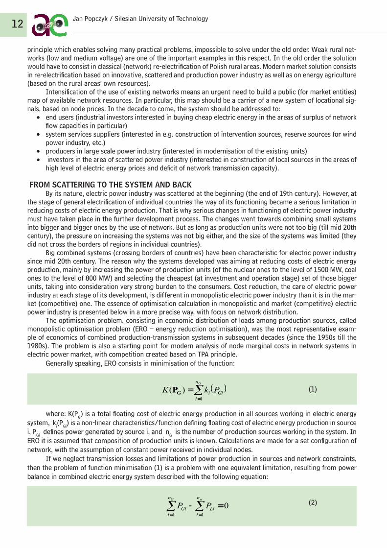
The optimisation problem, consisting in economic distribution of loads among production sources, called monopolistic optimisation problem (ERO – energy reduction optimisation), was the most representative exam-ple of economics of combined production-transmission systems in subsequent decades (since the 1950s till the 1980s). The problem is also a starting point for modern analysis of node marginal costs in network systems in electric power market, with competition created based on TPA principle.
Generally speaking, ERO consists in minimisation of the function:
(1)
where: K(PG) is a total floating cost of electric energy production in all sources working in electric energy system, ki(PGi) is a non-linear characteristics/function defining floating cost of electric energy production in source i, PGi defines power generated by source i, and nG is the number of production sources working in the system. In ERO it is assumed that composition of production units is known. Calculations are made for a set configuration of network, with the assumption of constant power received in individual nodes.
If we neglect transmission losses and limitations of power production in sources and network constraints, then the problem of function minimisation (1) is a problem with one equivalent limitation, resulting from power balance in combined electric energy system described with the following equation:
(2)
Zadanie ERO polega ogólnie na minimalizacji funkcji:
Gn
i
Gii PkK1
)( GP (1)
gdzie: K(PG) jest całkowitym zmiennym kosztem wytwarzania energii elektrycznej we
wszystkich źródłach pracujących w systemie elektroenergetycznym, ki(PGi) jest nieliniową charakterystyką/funkcją określającą zmienny koszt wytwarzania energii elektrycznej w źródle
i, PGi określa moc generowaną przez źródło i, natomiast nG jest liczbą źródeł wytwórczych
pracujących w systemie. W zadaniu ERO zakłada się, że znany jest skład jednostek
wytwórczych. Obliczenia wykonuje się dla ustalonej konfiguracji sieci przy założeniu stałej
mocy odbieranej w poszczególnych węzłach.
Jeśli pominąć straty przesyłowe, a także ograniczenia wytwarzania mocy w źródłach
oraz ograniczenia sieciowe, to zadanie minimalizacji funkcji (1) jest zadaniem z jednym
ograniczeniem równościowym, wynikającym z bilansu mocy w połączonym systemie
elektroenergetycznym określonym równaniem:
011
wG n
i
Li
n
i
Gi PP (2)
gdzie PLi oznacza moc czynną odbieraną w węźle i, a nw oznacza liczbę węzłów w sieci.
Zadanie to można rozwiązać analitycznie, wykorzystując w tym celu odpowiednio utworzoną funkcję Lagrange’a.
W rzeczywistości zadanie minimalizacji funkcji (1) ma oprócz ograniczenia
równościowego (2), uzupełnionego o straty mocy w sieci, trzy rodzaje ograniczeń
nierównościowych. Są to ograniczenia: górne i dolne mocy źródeł wytwórczych, górne
przepustowości linii (ograniczenia prądowe lub inaczej gałęziowe, dotyczące linii i
transformatorów) oraz górne i dolne napięć w węzłach sieci elektroenergetycznej
(ograniczenia napięciowe lub inaczej węzłowe). Do rozwiązania zadania z ograniczeniami
nierównościowymi (metodą iteracyjną) wykorzystuje się twierdzenie Kuhna-Tuckera.
Z ekonomicznego punktu widzenia podstawowe znaczenie w zadaniu minimalizacji
funkcji (1) mają charakterystyki/funkcje określające zmienne koszty wytwarzania energii
elektrycznej w poszczególnych źródłach wytwórczych. W praktyce koszty te na ogół określało się w przeszłości dla każdego źródła na podstawie jego technicznej charakterystyki
sprawności, wyznaczonej pomiarowo, i przeciętnej ceny jednostkowej paliwa. Jeszcze
częściej minimalizację kosztu w równaniu (1) zastępowało się minimalizacją ilości zużytego
paliwa. Generalną zasadą w monopolistycznej elektroenergetyce było przy tym stosowanie w
rachunku optymalizacyjnym kosztów przeciętnych. Trzeba natomiast pamiętać, że rynek
konkurencyjny działa, opierając się na kosztach krańcowych.
Według klasycznej definicji krótkookresowy koszt krańcowy energii elektrycznej w
węźle i (Short Run Marginal Cost – SRMC), nazywany dalej także krótkookresową ceną węzłową (Locational Marginal Price – LMP), jest równy minimalnej zmianie całkowitego
zmiennego kosztu wytwarzania energii w systemie, spowodowanej zmianą zapotrzebowania
w tym węźle. W warunkach polskiego rynku energii elektrycznej przez pojęcie „krótki okres”
rozumie się zwykle okres równy jednej godzinie. W związku z tym, w danej godzinie miarą energii odebranej/wygenerowanej w węźle i może być stała moc czynna. Definicję krótkookresowego kosztu węzłowego można zatem zapisać za pomocą zależności:
6
12 Jan Popczyk / Silesian University of Technology
where PLi means active power received in node i, and nw means the number of nodes in the network. The problem can be solved analytically, by the use of specially created Lagrange function.
In reality, apart from the equivalent constraint (2), supplemented by power losses in the network, the func-tion minimisation problem has three types of non-equivalent constraints. They are: upper and lower limitations of power of production sources, upper limitations of line flowing capacity (current limitations or other branch limitations of the line and transformers) and upper and lower constraints of voltages in nodes of electric energy network (voltage or other node limitations). Kuhn-Tucker theorem is used to solve the problem of non-equivalent limitations (by the use of iterative method).
From the economic point of view, characteristics/functions defining floating costs of electric energy pro-duction in individual production sources are of fundamental significance in function minimisation problem (1). In practice, in the past, the costs were usually defined for each source, based on its technical efficiency characteris-tics, set by measurement, and average unit price of fuel. Even more often, cost minimisation in equation (1) was replaced with minimisation of the fuel used. And using average costs in optimisation calculation was a general rule in monopolistic electric power industry. But it must be remembered that competitive market functions based on marginal costs.
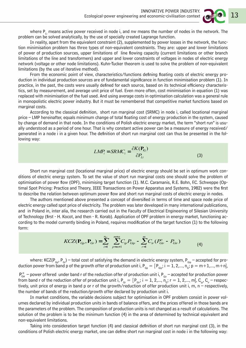
According to the classical definition, short run marginal cost (SRMC) in node i, called locational marginal price – LMP hereinafter, equals minimum change of total floating cost of energy production in the system, caused by change of demand in that node. In the conditions of Polish electric energy market, the term “short run” is usu-ally understood as a period of one hour. That is why constant active power can be a measure of energy received/generated in a node i in a given hour. The definition of short run marginal cost can thus be presented in the fol-lowing way:
(3)
Short run marginal cost (locational marginal price) of electric energy should be set in optimum work con-ditions of electric energy system. To set the value of short run marginal costs one should solve the problem of optimisation of power flow (OPF), minimising target function (1). M.C. Caramanis, R.E. Bohn, F.C. Schweppe (Op-timal Spot Pricing: Practice and Theory, IEEE Transactions on Power Apparatus and Systems, 1982) were the first to describe the relation between optimum power flow and short run marginal costs of electric energy in nodes.
The authors mentioned above presented a concept of diversified in terms of time and space node price of electric energy called spot price of electricity. The problem was later developed in many international publications, and in Poland in, inter alia, the research carried out in the Faculty of Electrical Engineering of Silesian University of Technology (first - H. Kocot, and then - R. Korab). Application of OPF problem in energy market, functioning ac-cording to the model currently binding in Poland, requires modification of the target function (1) to the following form:
(4)
where: KCZ(PGp, PGr) – total cost of satisfying the demand in electric energy system, PGip – accepted for pro-duction power from band p of the growth offer of production unit i, PGp = [PGip; i = 1, 2,..., nG; p = m+1,..., m+n],
oGirP – power offered under band r of the reduction offer of production unit i, PGir – accepted for production power
from band r of the reduction offer of production unit i, PGr = [PGir; i = 1, 2,..., nG; r = 1, 2,..., m], Cip, Cir – respec-tively, unit price of energy in band p or r of the growth/reduction of offer production unit i, m, n – respectively, the number of bands of the reduction/growth offer declared by production unit i.
In market conditions, the variable decisions subject for optimisation in OPF problem consist in power vol-umes declared by individual production units in bands of balance offers, and the prices offered in those bands are the parameters of the problem. The composition of production units is not changed as a result of calculations. The solution of the problem is to be the minimum function (4) in the area of determined by technical equivalent and non-equivalent limitations.
Taking into consideration target function (4) and classical definition of short run marginal cost (3), in the conditions of Polish electric energy market, one can define short run marginal cost in node i in the following way:
Li
iiP
KSRMCLMP
)( GP(3)
Krótkookresowy koszt krańcowy energii elektrycznej (krótkookresowa cena węzłowa)
powinien zostać wyznaczony w optymalnym stanie pracy systemu elektroenergetycznego. W
celu określenia wartości krótkookresowych kosztów węzłowych należy rozwiązać zadanie
optymalizacji rozpływu mocy OPF, minimalizujące funkcję celu (1). Po raz pierwszy w
literaturze światowej związek między optymalnym rozpływem mocy a krótkookresowymi
kosztami krańcowymi energii elektrycznej w węzłach sieci opisali M.C. Caramanis, R.E.
Bohn, F.C. Schweppe (Optimal Spot Pricing: Practice and Theory, IEEE Transactions on
Power Apparatus and Systems, 1982).
Wymienieni autorzy przedstawili koncepcję zróżnicowanej czasowo i przestrzennie
węzłowej ceny energii elektrycznej nazwanej spot price of electricity. W późniejszym okresie
za granicą tematyka ta została znacznie rozwinięta w wielu opracowaniach, zaś w Polsce
m.in. w pracach prowadzonych na Wydziale Elektrycznym Politechniki Śląskiej (najpierw H.
Kocot, następnie R. Korab). Zastosowanie zadania OPF na rynku energii, funkcjonującym
według modelu aktualnie obowiązującego w Polsce, wymaga modyfikacji funkcji celu (1) do
postaci:
Gn
i
m
r
Gir
o
Girir
nm
mp
GipipGrGp PPCPCKCZ1 11
)(),( PP (4)
gdzie: KCZ(PGp, PGr) – całkowity koszt pokrycia zapotrzebowania w systemie
elektroenergetycznym, PGip – zaakceptowana do produkcji moc z pasma p oferty przyrostowej
jednostki wytwórczej i, PGp = [PGip; i = 1, 2,..., nG; p = m+1,..., m+n], o
GirP – moc oferowana
w ramach pasma r oferty redukcyjnej jednostki wytwórczej i, PGir – zaakceptowana do
produkcji moc z pasma r oferty redukcyjnej jednostki wytwórczej i, PGr = [PGir; i = 1, 2,..., nG;
r = 1, 2,..., m], Cip, Cir – odpowiednio jednostkowa cena energii w paśmie p lub r oferty
przyrostowej/redukcyjnej jednostki wytwórczej i, m, n – odpowiednio liczba pasm oferty
redukcyjnej/przyrostowej zadeklarowanych przez jednostkę wytwórczą i.
Zmiennymi decyzyjnymi podlegającymi optymalizacji w zadaniu OPF w warunkach
rynkowych są wielkości mocy deklarowane przez poszczególne jednostki wytwórcze w pasmach
ofert bilansujących, natomiast ceny oferowane w tych pasmach są parametrami zadania. Skład
jednostek wytwórczych nie ulega zmianie w wyniku przeprowadzenia obliczeń. W zadaniu tym
poszukuje się minimum funkcji (4) w obszarze określonym przez techniczne ograniczenia
równościowe i nierównościowe.
Uwzględniając funkcję celu (4) oraz klasyczną definicję krótkookresowego kosztu
krańcowego (3), w warunkach polskiego rynku energii elektrycznej, krótkookresowy koszt
krańcowy w węźle i można zdefiniować następująco:
Li
GrGp
iiP
KCZSRMCLMP
),( PP(5)
Krótkookresowy koszt węzłowy (5) można rozłożyć na składniki o prostej interpretacji
fizykalnej, są to: koszt węzłowy energii elektrycznej, czynnej w węźle bilansującym, koszt
7
INNOVATIVE POWER INDUSTRY. Ecological-power engineering and economic-civilisation context 13
Li
iiP
KSRMCLMP
)( GP(3)
Krótkookresowy koszt krańcowy energii elektrycznej (krótkookresowa cena węzłowa)
powinien zostać wyznaczony w optymalnym stanie pracy systemu elektroenergetycznego. W
celu określenia wartości krótkookresowych kosztów węzłowych należy rozwiązać zadanie
optymalizacji rozpływu mocy OPF, minimalizujące funkcję celu (1). Po raz pierwszy w
literaturze światowej związek między optymalnym rozpływem mocy a krótkookresowymi
kosztami krańcowymi energii elektrycznej w węzłach sieci opisali M.C. Caramanis, R.E.
Bohn, F.C. Schweppe (Optimal Spot Pricing: Practice and Theory, IEEE Transactions on
Power Apparatus and Systems, 1982).
Wymienieni autorzy przedstawili koncepcję zróżnicowanej czasowo i przestrzennie
węzłowej ceny energii elektrycznej nazwanej spot price of electricity. W późniejszym okresie
za granicą tematyka ta została znacznie rozwinięta w wielu opracowaniach, zaś w Polsce
m.in. w pracach prowadzonych na Wydziale Elektrycznym Politechniki Śląskiej (najpierw H.
Kocot, następnie R. Korab). Zastosowanie zadania OPF na rynku energii, funkcjonującym
według modelu aktualnie obowiązującego w Polsce, wymaga modyfikacji funkcji celu (1) do
postaci:
Gn
i
m
r
Gir
o
Girir
nm
mp
GipipGrGp PPCPCKCZ1 11
)(),( PP (4)
gdzie: KCZ(PGp, PGr) – całkowity koszt pokrycia zapotrzebowania w systemie
elektroenergetycznym, PGip – zaakceptowana do produkcji moc z pasma p oferty przyrostowej
jednostki wytwórczej i, PGp = [PGip; i = 1, 2,..., nG; p = m+1,..., m+n], o
GirP – moc oferowana
w ramach pasma r oferty redukcyjnej jednostki wytwórczej i, PGir – zaakceptowana do
produkcji moc z pasma r oferty redukcyjnej jednostki wytwórczej i, PGr = [PGir; i = 1, 2,..., nG;
r = 1, 2,..., m], Cip, Cir – odpowiednio jednostkowa cena energii w paśmie p lub r oferty
przyrostowej/redukcyjnej jednostki wytwórczej i, m, n – odpowiednio liczba pasm oferty
redukcyjnej/przyrostowej zadeklarowanych przez jednostkę wytwórczą i.
Zmiennymi decyzyjnymi podlegającymi optymalizacji w zadaniu OPF w warunkach
rynkowych są wielkości mocy deklarowane przez poszczególne jednostki wytwórcze w pasmach
ofert bilansujących, natomiast ceny oferowane w tych pasmach są parametrami zadania. Skład
jednostek wytwórczych nie ulega zmianie w wyniku przeprowadzenia obliczeń. W zadaniu tym
poszukuje się minimum funkcji (4) w obszarze określonym przez techniczne ograniczenia
równościowe i nierównościowe.
Uwzględniając funkcję celu (4) oraz klasyczną definicję krótkookresowego kosztu
krańcowego (3), w warunkach polskiego rynku energii elektrycznej, krótkookresowy koszt
krańcowy w węźle i można zdefiniować następująco:
Li
GrGp
iiP
KCZSRMCLMP
),( PP(5)
Krótkookresowy koszt węzłowy (5) można rozłożyć na składniki o prostej interpretacji
fizykalnej, są to: koszt węzłowy energii elektrycznej, czynnej w węźle bilansującym, koszt
7
(5)
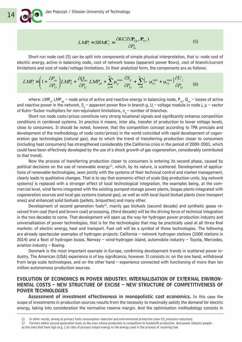
Short run node cost (5) can be split into components of simple physical interpretation, that is: node cost of electric energy, active in balancing node, cost of network losses (apparent power flows), cost of branch/current limitations and cost of node/voltage limitations. In their analytical form, the components are as follows:
(6)
where: LMPb, LMPqb – node price of active and reactive energy in balancing node, Pstr, Qstr – losses of active and reactive power in the network, Sg – apparent power flow in branch g, Uj – voltage module in node j, m – vector of Kuhn–Tucker multipliers for non-equivalent limitations, ng – number of branches.
Short run node costs/prices constitute very strong locational signals and significantly enhance competition conditions in combined systems. In practice it means, inter alia, transfer of production to lower voltage levels, close to consumers. It should be noted, however, that the competition concept according to TPA principle and development of the methodology of node costs/prices) in the world coincided with rapid development of cogen-eration gas technologies (natural gas), due to which the trend of transferring production closer to consumers (including heat consumers) has strengthened considerably (the California crisis in the period of 2000–2001, which could have been effectively developed by the use of a shock growth of gas cogeneration, considerably contributed to that trend).
Now the process of transferring production closer to consumers is entering its second phase, caused by political decisions on the use of renewable energy11, which, by its nature, is scattered. Development of applica-tions of renewable technologies, seen jointly with the systems of their technical control and market management, clearly leads to qualitative changes. That is to say that economic effect of scale (big production units, big network systems) is replaced with a stronger effect of local technological integration, the examples being, at the com-mercial level, wind farms integrated with the existing pumped-storage power plants, biogas plants integrated with cogeneration sources and local gas systems (natural gas), as well as with local liquid biofuel plants (now transport ones) and enhanced solid biofuels (pellets, briquettes) and many other.
Development of second generation fuels12, mainly gas biofuels (second decade) and synthetic gases re-ceived from coal (hard and brown coal) processing, (third decade) will be the driving force of technical integration in the two decades to come. That development will open up the way for hydrogen power production industry and universalisation of power technologies, that is for the technologies that may be practically used at all three final markets: of electric energy, heat and transport. Fuel cell will be a symbol of those technologies. The following are already spectacular examples of hydrogen projects: California – network hydrogen stations (1000 stations in 2014) and a fleet of hydrogen buses, Norway – wind-hydrogen island, automobile industry – Toyota, Mercedes, aviation industry – Boeing.
Denmark is the most important example in Europe, confirming development trends in scattered power in-dustry. The American (USA) experience is of key significance, however. It consists in: on the one hand, withdrawal from large scale technologies, and on the other hand – experience connected with functioning of more than ten million autonomous production sources.
EVOLUTION OF ECONOMICS IN POWER INDUSTRY. INTERNALISATION OF EXTERNAL ENVIRON-MENTAL COSTS – NEW STRUCTURE OF EXCISE – NEW STRUCTURE OF COMPETITIVENESS OF POWER TECHNOLOGIES
Assessment of investment effectiveness in monopolistic cost economics. In this case the scope of investments in production sources results from the necessity to maximally satisfy the demand for electric energy, taking into consideration the normative reserve margin. And the optimisation methodology consists in
11 In other words, aiming at primary fuels consumption reduction and environmental protection (now CO2 emission reduction).12 Farmers define second generation fuels as the ones whose production is competitive to foodstuffs production. And power industry people - as the ones that have high (e.g. 1.6) ratio of process output energy to the energy used in the process of receiving fuel.
strat sieciowych (od przepływu mocy pozornych), koszt ograniczeń gałęziowych/prądowych i
koszt ograniczeń węzłowych/napięciowych. W formie analitycznej składniki te mają postać:
wg n
j Li
j
UjUj
n
g Li
g
gqb
Li
strb
Li
stri
P
U
P
SLMP
P
QLMP
P
PLMP
11
1 maxminmax µµµ (6)
gdzie: LMPb, LMPqb – cena węzłowa energii czynnej i biernej w węźle bilansującym, Pstr, Qstr
– straty mocy czynnej i biernej w sieci, Sg – przepływ mocy pozornej w gałęzi g, Uj – moduł napięcia w węźle j, µ – wektor mnożników Kuhna–Tuckera dla ograniczeń
nierównościowych, ng – liczba gałęzi.
Krótkookresowe koszty/ceny węzłowe stanowią bardzo silne sygnały lokalizacyjne i
znacznie polepszają uwarunkowania dla konkurencji w połączonych systemach. W praktyce
oznacza to między innymi przenoszenie wytwarzania na niższe poziomy napięciowe, bliżej
odbiorców. Trzeba przy tym podkreślić, że koncepcja konkurencji według zasady TPA i
rozwój metodyki kosztów/cen węzłowych) na świecie zbiegły się w czasie z gwałtownym
rozwojem gazowych technologii kogeneracyjnych (na gaz ziemny). Dzięki temu trend
przenoszenia wytwarzania bliżej odbiorców (u których są odbiory ciepła) niezwykle się wzmocnił (kryzys kalifornijski w latach 2000–2001, który można było rozwiązać efektywnie
za pomocą szokowego wzrostu kogeneracji gazowej, znacznie się do tego przyczynił).
Obecnie proces przenoszenia wytwarzania bliżej odbiorców wchodzi w drugą fazę, a
powodują ją decyzje polityczne dotyczące wykorzystania energetyki odnawialnej11, która z
natury jest rozproszona. Rozwój zastosowań technologii odnawialnych, widzianych łącznie z
systemami ich sterowania technicznego i zarządzania rynkowego, w sposób widoczny
prowadzi do nowych zmian jakościowych. Mianowicie, ekonomiczny efekt skali (wielkie
bloki wytwórcze, wielkie systemy sieciowe) jest wypierany przez silniejszy efekt lokalnej
integracji technologicznej. Przykładami takiej integracji są już, na poziomie komercyjnym,
farmy wiatrowe integrowane z istniejącymi elektrowniami szczytowo-pompowymi,
biogazownie integrowane ze źródłami kogeneracyjnymi i lokalnymi systemami gazowymi
(gazu ziemnego), a także z lokalnymi wytwórniami biopaliw płynnych (obecnie
transportowych) i ulepszonych biopaliw stałych (pelety, brykiety) i wiele innych.
Siłą napędową integracji technologicznej w kolejnych dwóch dekadach będzie rozwój
paliw drugiej generacji12, przede wszystkim biopaliw gazowych (druga dekada) i gazów
syntezowych otrzymywanych w procesie przeróbki węgla, zarówno kamiennego, jak i
brunatnego (trzecia dekada). Rozwój ten otworzy drogę do energetyki wodorowej i
uniwersalizacji technologii energetycznych, tzn. do takich technologii, które będą się praktycznie nadawać do wykorzystania na wszystkich trzech rynkach końcowych: energii
elektrycznej, ciepła i transportu. Symbolem tych technologii będzie ogniwo paliwowe.
Spektakularnymi przykładami projektów wodorowych już obecnie są: Kalifornia – sieć stacji
wodorowych (1000 stacji w 2014 roku) i flota autobusów wodorowych, Norwegia – wyspa
wiatrowo-wodorowa, przemysł samochodowy – Toyota, Mercedes, lotnictwo – Boeing.
Najważniejszym przykładem w Europie, potwierdzającym siłę trendów rozwojowych
energetyki rozproszonej, jest Dania. Jednak kluczowe znaczenie mają doświadczenia
amerykańskie (USA). Na te ostatnie doświadczenia składają się: odwrót od technologii
11 Inaczej, dążenie do obniżenia zużycia paliw pierwotnych i ochrona środowiska (obecnie redukcja emisji CO2).12 Rolnicy definiują paliwa drugiej generacji jako te, których produkcja nie jest konkurencyjna względem
produkcji żywności. Energetycy natomiast jako te, które mają wysoki (np. 1,6) stosunek energii na wyjściu z
procesu do energii włożonej w procesie pozyskiwania paliwa.
8
Li
iiP
KSRMCLMP
)( GP(3)
Krótkookresowy koszt krańcowy energii elektrycznej (krótkookresowa cena węzłowa)
powinien zostać wyznaczony w optymalnym stanie pracy systemu elektroenergetycznego. W
celu określenia wartości krótkookresowych kosztów węzłowych należy rozwiązać zadanie
optymalizacji rozpływu mocy OPF, minimalizujące funkcję celu (1). Po raz pierwszy w
literaturze światowej związek między optymalnym rozpływem mocy a krótkookresowymi
kosztami krańcowymi energii elektrycznej w węzłach sieci opisali M.C. Caramanis, R.E.
Bohn, F.C. Schweppe (Optimal Spot Pricing: Practice and Theory, IEEE Transactions on
Power Apparatus and Systems, 1982).
Wymienieni autorzy przedstawili koncepcję zróżnicowanej czasowo i przestrzennie
węzłowej ceny energii elektrycznej nazwanej spot price of electricity. W późniejszym okresie
za granicą tematyka ta została znacznie rozwinięta w wielu opracowaniach, zaś w Polsce
m.in. w pracach prowadzonych na Wydziale Elektrycznym Politechniki Śląskiej (najpierw H.
Kocot, następnie R. Korab). Zastosowanie zadania OPF na rynku energii, funkcjonującym
według modelu aktualnie obowiązującego w Polsce, wymaga modyfikacji funkcji celu (1) do
postaci:
Gn
i
m
r
Gir
o
Girir
nm
mp
GipipGrGp PPCPCKCZ1 11
)(),( PP (4)
gdzie: KCZ(PGp, PGr) – całkowity koszt pokrycia zapotrzebowania w systemie
elektroenergetycznym, PGip – zaakceptowana do produkcji moc z pasma p oferty przyrostowej
jednostki wytwórczej i, PGp = [PGip; i = 1, 2,..., nG; p = m+1,..., m+n], o
GirP – moc oferowana
w ramach pasma r oferty redukcyjnej jednostki wytwórczej i, PGir – zaakceptowana do
produkcji moc z pasma r oferty redukcyjnej jednostki wytwórczej i, PGr = [PGir; i = 1, 2,..., nG;
r = 1, 2,..., m], Cip, Cir – odpowiednio jednostkowa cena energii w paśmie p lub r oferty
przyrostowej/redukcyjnej jednostki wytwórczej i, m, n – odpowiednio liczba pasm oferty
redukcyjnej/przyrostowej zadeklarowanych przez jednostkę wytwórczą i.
Zmiennymi decyzyjnymi podlegającymi optymalizacji w zadaniu OPF w warunkach
rynkowych są wielkości mocy deklarowane przez poszczególne jednostki wytwórcze w pasmach
ofert bilansujących, natomiast ceny oferowane w tych pasmach są parametrami zadania. Skład
jednostek wytwórczych nie ulega zmianie w wyniku przeprowadzenia obliczeń. W zadaniu tym
poszukuje się minimum funkcji (4) w obszarze określonym przez techniczne ograniczenia
równościowe i nierównościowe.
Uwzględniając funkcję celu (4) oraz klasyczną definicję krótkookresowego kosztu
krańcowego (3), w warunkach polskiego rynku energii elektrycznej, krótkookresowy koszt
krańcowy w węźle i można zdefiniować następująco:
Li
GrGp
iiP
KCZSRMCLMP
),( PP(5)
Krótkookresowy koszt węzłowy (5) można rozłożyć na składniki o prostej interpretacji
fizykalnej, są to: koszt węzłowy energii elektrycznej, czynnej w węźle bilansującym, koszt
7
14 Jan Popczyk / Silesian University of Technology
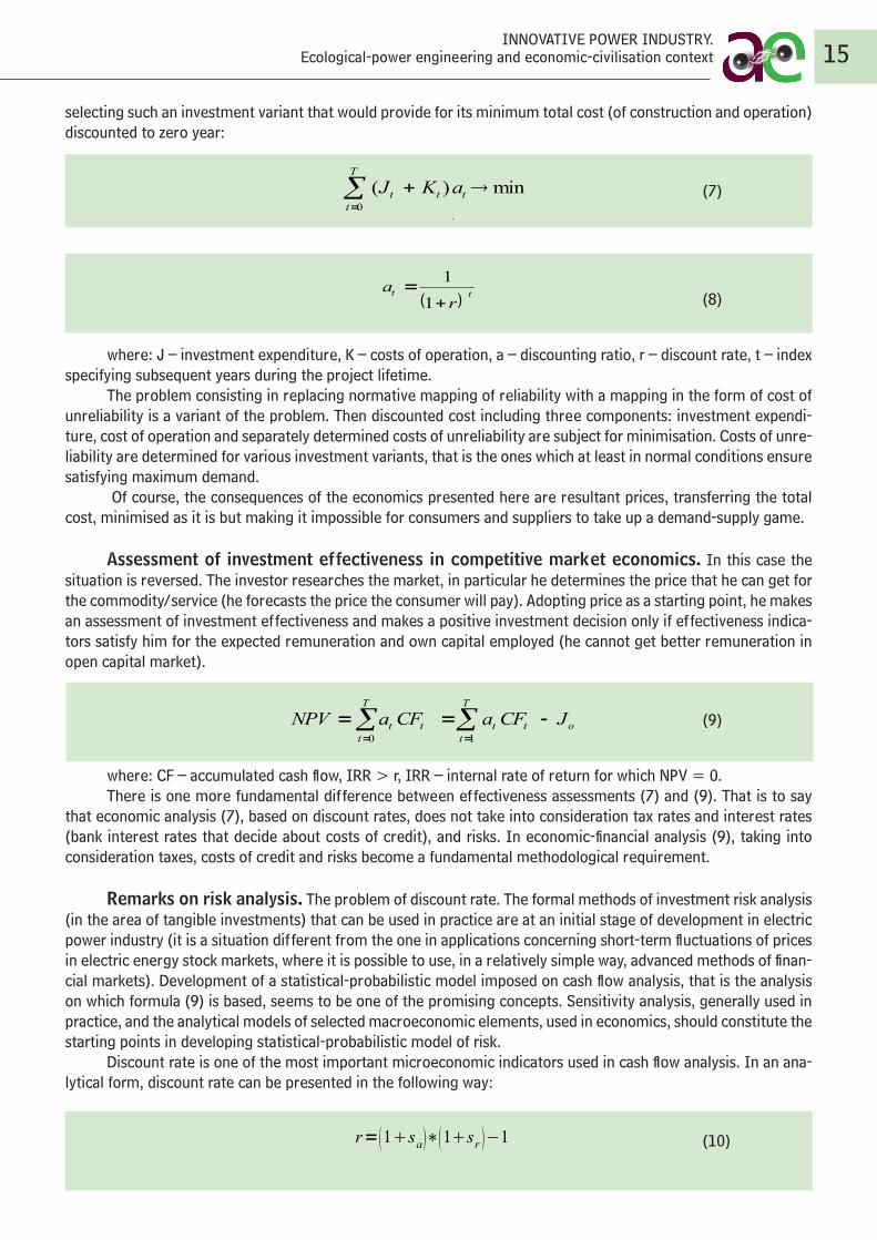
selecting such an investment variant that would provide for its minimum total cost (of construction and operation) discounted to zero year:
(7)
(8)
where: J – investment expenditure, K – costs of operation, a – discounting ratio, r – discount rate, t – index specifying subsequent years during the project lifetime.
The problem consisting in replacing normative mapping of reliability with a mapping in the form of cost of unreliability is a variant of the problem. Then discounted cost including three components: investment expendi-ture, cost of operation and separately determined costs of unreliability are subject for minimisation. Costs of unre-liability are determined for various investment variants, that is the ones which at least in normal conditions ensure satisfying maximum demand.
Of course, the consequences of the economics presented here are resultant prices, transferring the total cost, minimised as it is but making it impossible for consumers and suppliers to take up a demand-supply game.
Assessment of investment effectiveness in competitive market economics. In this case the situation is reversed. The investor researches the market, in particular he determines the price that he can get for the commodity/service (he forecasts the price the consumer will pay). Adopting price as a starting point, he makes an assessment of investment effectiveness and makes a positive investment decision only if effectiveness indica-tors satisfy him for the expected remuneration and own capital employed (he cannot get better remuneration in open capital market).
(9)
where: CF – accumulated cash flow, IRR > r, IRR – internal rate of return for which NPV = 0.There is one more fundamental difference between effectiveness assessments (7) and (9). That is to say
that economic analysis (7), based on discount rates, does not take into consideration tax rates and interest rates (bank interest rates that decide about costs of credit), and risks. In economic-financial analysis (9), taking into consideration taxes, costs of credit and risks become a fundamental methodological requirement.
Remarks on risk analysis. The problem of discount rate. The formal methods of investment risk analysis (in the area of tangible investments) that can be used in practice are at an initial stage of development in electric power industry (it is a situation different from the one in applications concerning short-term fluctuations of prices in electric energy stock markets, where it is possible to use, in a relatively simple way, advanced methods of finan-cial markets). Development of a statistical-probabilistic model imposed on cash flow analysis, that is the analysis on which formula (9) is based, seems to be one of the promising concepts. Sensitivity analysis, generally used in practice, and the analytical models of selected macroeconomic elements, used in economics, should constitute the starting points in developing statistical-probabilistic model of risk.
Discount rate is one of the most important microeconomic indicators used in cash flow analysis. In an ana-lytical form, discount rate can be presented in the following way:
(10)
wielkoskalowych z jednej strony, z drugiej natomiast doświadczenia związane z
funkcjonowaniem kilkunastu milionów autonomicznych źródeł wytwórczych.
Ewolucja ekonomiki w energetyce. Internalizacja kosztów zewnętrznych środowiska –
nowa struktura podatku akcyzowego – nowa struktura konkurencyjności technologii
energetycznych
Ocena efektywności inwestycji w monopolistycznej ekonomice kosztowej. W tym
przypadku zakres inwestycji w źródła wytwórcze wynika z konieczności pokrycia
maksymalnego zapotrzebowania na energię elektryczną, z uwzględnieniem normatywnego
marginesu rezerwy. Metodyka optymalizacyjna polega zaś na wyborze wariantu
inwestycyjnego, zapewniającego jego minimalny koszt łączny (budowy i eksploatacji)
zdyskontowany na rok zerowy:
T
t
ttt aKJ0
min)( (7)
tt
ra
1
1(8)
gdzie: J – nakłady inwestycyjne, K – koszty eksploatacji, a – współczynnik dyskontujący, r –
stopa dyskonta, t – indeks oznaczający kolejne lata w okresie życia projektu.
Odmianą zadania jest zadanie polegające na zastąpieniu normatywnego odwzorowania
niezawodności odwzorowaniem w postaci kosztu zawodności. Wówczas minimalizacji
podlega zdyskontowany koszt obejmujący trzy składniki: nakłady inwestycyjne, koszty
eksploatacyjne i odrębnie określone koszty zawodności. Koszty zawodności określa się dla
zróżnicowanych wariantów inwestycyjnych, przy tym takich, które przynajmniej w
warunkach normalnych zapewniają pokrycie maksymalnego zapotrzebowania.
Oczywiście, konsekwencją przedstawionej tu ekonomiki są wynikowe ceny,
przenoszące łączny koszt, wprawdzie zminimalizowany, ale uniemożliwiający odbiorcom i
dostawcom podjęcie gry popytowo-podażowej.
Ocena efektywności inwestycji w konkurencyjnej ekonomice rynkowej. W tym przypadku
następuje odwrócenie sytuacji. Inwestor bada rynek, w szczególności określa cenę, jaką może
uzyskać za towar/usługę (prognozuje cenę, którą zapłaci odbiorca). Przyjmując tę cenę za
punkt wyjścia, dokonuje oceny efektywności inwestycji i podejmuje pozytywną decyzję inwestycyjną tylko wówczas, jeśli wskaźniki efektywności są dla niego satysfakcjonujące pod
względem oczekiwanego wynagrodzenia i zaangażowanego kapitału własnego (nie może
uzyskać lepszego wynagrodzenia na otwartym rynku kapitałowym).
T
t
ott
T
t
tt JCFaCFaNPV10
(9)
gdzie: CF – skumulowany przepływ finansowy (cash flow), IRR > r, IRR – wewnętrzna stopa
zwrotu, dla której NPV = 0.
Istnieje jeszcze jedna fundamentalna różnica między ocenami efektywności (7) i (9).
Mianowicie, w analizie ekonomicznej (7), której podstawą są stopy dyskontowe, nie
uwzględnia się stóp podatkowych i stóp procentowych (stóp bankowych decydujących o
9
INNOVATIVE POWER INDUSTRY. Ecological-power engineering and economic-civilisation context 15
wielkoskalowych z jednej strony, z drugiej natomiast doświadczenia związane z
funkcjonowaniem kilkunastu milionów autonomicznych źródeł wytwórczych.
Ewolucja ekonomiki w energetyce. Internalizacja kosztów zewnętrznych środowiska –
nowa struktura podatku akcyzowego – nowa struktura konkurencyjności technologii
energetycznych
Ocena efektywności inwestycji w monopolistycznej ekonomice kosztowej. W tym
przypadku zakres inwestycji w źródła wytwórcze wynika z konieczności pokrycia
maksymalnego zapotrzebowania na energię elektryczną, z uwzględnieniem normatywnego
marginesu rezerwy. Metodyka optymalizacyjna polega zaś na wyborze wariantu
inwestycyjnego, zapewniającego jego minimalny koszt łączny (budowy i eksploatacji)
zdyskontowany na rok zerowy:
T
t
ttt aKJ0
min)( (7)
tt
ra
1
1(8)
gdzie: J – nakłady inwestycyjne, K – koszty eksploatacji, a – współczynnik dyskontujący, r –
stopa dyskonta, t – indeks oznaczający kolejne lata w okresie życia projektu.
Odmianą zadania jest zadanie polegające na zastąpieniu normatywnego odwzorowania
niezawodności odwzorowaniem w postaci kosztu zawodności. Wówczas minimalizacji
podlega zdyskontowany koszt obejmujący trzy składniki: nakłady inwestycyjne, koszty
eksploatacyjne i odrębnie określone koszty zawodności. Koszty zawodności określa się dla
zróżnicowanych wariantów inwestycyjnych, przy tym takich, które przynajmniej w
warunkach normalnych zapewniają pokrycie maksymalnego zapotrzebowania.
Oczywiście, konsekwencją przedstawionej tu ekonomiki są wynikowe ceny,
przenoszące łączny koszt, wprawdzie zminimalizowany, ale uniemożliwiający odbiorcom i
dostawcom podjęcie gry popytowo-podażowej.
Ocena efektywności inwestycji w konkurencyjnej ekonomice rynkowej. W tym przypadku
następuje odwrócenie sytuacji. Inwestor bada rynek, w szczególności określa cenę, jaką może
uzyskać za towar/usługę (prognozuje cenę, którą zapłaci odbiorca). Przyjmując tę cenę za
punkt wyjścia, dokonuje oceny efektywności inwestycji i podejmuje pozytywną decyzję inwestycyjną tylko wówczas, jeśli wskaźniki efektywności są dla niego satysfakcjonujące pod
względem oczekiwanego wynagrodzenia i zaangażowanego kapitału własnego (nie może
uzyskać lepszego wynagrodzenia na otwartym rynku kapitałowym).
T
t
ott
T
t
tt JCFaCFaNPV10
(9)
gdzie: CF – skumulowany przepływ finansowy (cash flow), IRR > r, IRR – wewnętrzna stopa
zwrotu, dla której NPV = 0.
Istnieje jeszcze jedna fundamentalna różnica między ocenami efektywności (7) i (9).
Mianowicie, w analizie ekonomicznej (7), której podstawą są stopy dyskontowe, nie
uwzględnia się stóp podatkowych i stóp procentowych (stóp bankowych decydujących o
9
kosztach kredytów), a także ryzyk. W analizie ekonomiczno-finansowej (9) uwzględnienie
podatków, kosztów kredytów i ryzyk staje się podstawowym wymaganiem metodologicznym.
Uwagi dotyczące analizy ryzyka. Problem stopy dyskontowej. Formalne metody analizy
ryzyka inwestycyjnego (w obszarze inwestycji materialnych), nadające się do zastosowań
praktycznych, są w elektroenergetyce dopiero w początkowej fazie rozwoju (jest to inna
sytuacja niż w zastosowaniach dotyczących krótkookresowych wahań cen na rynkach
giełdowych energii elektrycznej, gdzie możliwe jest stosunkowo proste wykorzystanie
zaawansowanych metod z rynków finansowych). Jedną z koncepcji, którą można wskazać jako obiecującą, jest budowa modelu statystyczno-probabilistycznego nałożonego na analizę przepływów finansowych, czyli analizę, której podstawą jest wzór (9). Punktem wyjścia do
budowy modelu statystyczno-probabilistycznego ryzyka w tej koncepcji powinna być analiza
wrażliwości stosowana powszechnie w praktyce, a ponadto stosowane w ekonomii modele
analityczne wybranych wielkości makroekonomicznych.
Jedną z najważniejszych wielkości makroekonomicznych, wykorzystywanych w
analizie przepływów finansowych, jest stopa dyskontowa. Stopa ta w postaci analitycznej
może być wyrażona w sposób następujący:
r=1sa∗1s
r −1 (10)
gdzie: sa – jest kosztem alternatywnym kapitału (najczęściej równym oprocentowaniu
państwowych obligacji długoterminowych), sr – jest natomiast stopą ryzyka,
charakterystyczną dla danej działalności gospodarczej.
Stopa dyskontowa charakteryzuje kondycję gospodarki oraz jej stabilność w
długoterminowym horyzoncie inwestycyjnym i stanowi w szczególności podstawę decyzji
inwestycyjnych o kluczowym znaczeniu w sektorach o największej kapitałochłonności. Stopa
dyskontowa, jako parametr pozwalający uwzględnić zmianę wartości pieniądza w czasie, ma
zasadniczy wpływ na optymalną (dla danej gospodarki) strukturę nakładów inwestycyjnych
(rozłożonych w okresie inwestowania) oraz przyszłych kosztów eksploatacyjnych
(ponoszonych przez długi czas).
Jest jasne, że wysokie stopy dyskontowe, charakterystyczne dla słabych i niestabilnych
gospodarek, prowadzą do rozwiązań o niskich nakładach inwestycyjnych i wysokich kosztach
eksploatacyjnych, a niskie stopy odwrotnie – do rozwiązań o wysokich kosztach
inwestycyjnych i niskich kosztach eksploatacyjnych. Jeśli zatem pominąć ryzyko
technologiczne oraz ryzyko zmian cen paliw, to zastosowanie rachunku dyskonta powoduje,
że elektrownie wodne (i ogólnie źródła odnawialne energii elektrycznej), a także elektrownie
atomowe mają większe szanse zastosowania w USA i w Europie Zachodniej, natomiast
elektrownie gazowe (ewentualnie na ropę naftową) są bardziej właściwe dla Afryki i Ameryki
Południowej. Podobnie, niska stopa dyskontowa w USA i w Unii preferuje linie
elektroenergetyczne o dużych przekrojach przewodów roboczych (wyższych nakładach
inwestycyjnych, niższych kosztach strat mocy i energii), a wysoka stopa dyskontowa,
właściwa dla gospodarek krajów afrykańskich i południowoamerykańskich, prowadzi do
mniejszych przekrojów przewodów roboczych linii elektroenergetycznych.
Wybór stopy dyskontowej do zilustrowania problemu ryzyka w elektroenergetyce
rynkowej, i ogólnie na rynkach z wymaganą kapitałochłonną infrastrukturą, ma
charakterystyczne znaczenie z wielu innych punktów widzenia (poza punktem widzenia
związanym z techniką obliczeniową), z których dwa są najważniejsze. Po pierwsze, podejście
do stopy dyskontowej wyrażone za pomocą wzoru (10) wskazuje, że rynek będzie wymuszał zbliżanie się tradycyjnych metodologii ocen ekonomicznych materialnych inwestycji
10

where: sa – is an alternative cost of capital (usually equal to interest rate on long-term state bonds), sr – is a risk rate, characteristic for the given business.
Discount rate characterises the standing of the economy and its stability in long-term investment perspec-tive and in particular constitutes a basis for investment decisions of key significance in sectors of the biggest capi-tal consumption. As a parameter that enables taking into account change of money value in time, discount rate fundamentally affects optimum (for the given economy) structure of investment expenditure (distributed over investment time) and future operation costs (incurred over a long period of time).
It is clear that high discount rates, characteristic for weak and instable economies, lead to solutions of low investment expenditure and high operation cost, but low rates – just the opposite – to solutions of high investment costs and low operation costs. If one neglects technological risk and risk of change of fuel prices, then application of discount calculation provides better opportunities for existence of water power plants (and generally, renewable sources of electric energy), and nuclear power plants in USA and Western Europe. And gas power plants (or oil powered ones) are more proper for Africa and South America. Similarly, low discount rate in USA and in the Euro-pean Union prefers electric power lines of big cross-sections of working cables (of higher investment expenditure, lower costs of power and energy losses), and high discount rate, characteristic for the economies of African and South American countries, leads to smaller cross-sections of working cables of electric power lines.
The choice of a discount rate to illustrate the problem of risk in electric power market, and generally in the markets with the required capital consuming infrastructure, is of characteristic significance from many points of view (apart from the point of view connected with calculation technique), of which the following two are the most important ones. Firstly, the approach to discount rate expressed by formula (10) indicates that the market will be forcing similarity of traditional methodologies of economic assessments of material infrastructure invest-ments and the methodologies of assessing capital investments. It means, of course, universalisation and levelling as tendencies, profitability of infrastructure investments and profitability of the market expressed by the use of profitability of stock included in characteristic stock indexes, e.g. American indexes: industrial - Dow Jones In-dustrial Average, banking - Standard & Poor and technological - Nasdaq. In other words, in competitive markets infrastructure services it means a trend from economic account to financial account and from long-term account to short-term account. Secondly, formula (10) points out to a special task to be performed in terms of the neces-sary modernisation of regulation systems of infrastructure services markets. That is to say it is necessary for the regulators to develop immediately a basis for setting risk rate sr and determining its reference value, in network infrastructure in particular.
In the case of electric power industry, a challenge is posed also by determining risk rate sr, different for individual power technologies, e.g. for nuclear power industry13, for coal, gas, renewable energy industry and for pro-efficient technologies in the area of using electric energy. It is clear that market risk of building a traditional nuclear unit of 1500 MW, for PLN 10 billion differs from the risk of building a unit of 460 MW for PLN 1800 million, powered by hard coal, whose market is shrinking. And it is obvious that the latter is radically different from the risk of building a micro gas powered electric heat plant for PLN 1 million in a fast growing market of cogeneration scat-tered power industry. And finally, the situation in the market of pro-efficient technologies in the area of using elec-tric energy, where competition mechanisms have been in place for as long time and are stable, is also different.
REFERENCE COSTS/PRICES THAT TAKE INTO ACCOUNT INTERNALISATION OF EXTERNAL COSTS Fig 1 presents reference costs taking into account internalisation of external environmental costs, and also
the costs that can soon become a source of stranded costs, that is those of network and system services. A uni-form (product) internalisation of CO2 emission costs was adopted in the method used to estimate the presented reference costs. In the light of 3x20 Energy and Climate Package (specifying the total target of CO2 emission re-duction in all three final markets: electric energy, heat and transport), this method should surely be improved. The improvement should go towards using the thermo-ecological method connected with egzergy for internalisation of CO2 emission costs.
Despite the fact that Fig. 1 presents the change of competitiveness structure of electric energy technologies that seems to be shocking now, one must remember that it is only an introduction to what is going to happen in
13 The risk of nuclear power industry in macroeconomic terms (for example in inflation aspect), that is no longer in terms of big environmental disasters and costs of treatment of used fuel (still, to a great extent, outside the mechanism of internalisation), is becoming a subject of a serious public debate in USA [11].
16 Jan Popczyk / Silesian University of Technology

the decades to come. That is to say that the revolution in the area of fuels will cause a decline of the existing excise system and that a new one will be created. The current excise system, developed over decades, is, in particular, subordinated to the way of using fuels. In such a system, diesel fuel used for transport, for example, has a very high excise, but natural gas does not. The same diesel fuel put into a car, having a very high excise, has a much lower excise if it is used in cogeneration aggregate. There are many similar examples. The conclusion is unambigu-ous - the existing excise, characteristic for industrial society, is totally irrational in knowledge society, and it would be even more irrational in a hydrogen society (now it can by no means be justified for technological reasons, and is even corruptive in this aspect). That is why it is necessary to develop a new, uniform excise system from the scratch. It seems that the thermo-ecological method mentioned above, connected with egzergy, would be even more useful in this case.
Fig. 1. Reference costs for various electric energy technologies and for two values of CO2 emission allowances: 10 euro/ton and 40 euro/ton [8]Technologies: 1 – nuclear unit, transmission network, 2 – brown coal unit, transmission network, 3 – hard coal unit, transmission network, 4 – gas cogeneration source, 110 kV network, 5 – gas cogeneration source, MV network, 6 – gas cogeneration source, LV network, 7 – integrated wind-gas technology, 110 kV network, 8 – biomethane cogeneration source, MV network, 9 – small water power plant, MV network, 10 – fuel cell
Without going into methodological complexities, to illustrate the fact that the new economics changes the competitiveness structure of electric energy technologies, in particular makes large scale coal technologies non-competitive, it will present, apart from Fig. 1, a simplified estimation of unit cost for Łagisza unit under construc-tion of (supercritical, fluidal) 460 MW. The basic data, deciding about unit cost of electric energy supplied from that unit to end (averaged) user are as follows: investment expenditure – PLN 1.8 billion, net effectiveness – 42%, CO2 emission – 0.8 t/MWh, time of use of nominal power – 7000 h/year.
Individual components of unit cost of electric energy for end consumer for the above data are as follows: depreciation (for depreciation period of 30 years) – 20 PLN/MWh, cost of transferable capital (for IRR of 8%) – 60 PLN/MWh, cost of coal – 100 PLN/MWh, cost of CO2 emission allowances – 120 PLN/MWh, fixed costs variabled – 20 PLN/MWh, transfer charge – 100 PLN/MWh. And the total is 420 PLN/MWh. It is a cost very well correspond-ing with the upper level of the cost for technology 3 (matching Łagisza unit) in Fig. 1.
POWER INDUSTRY SQUEEZED INTO THE MECHANISM OF ECONOMIC CYCLES The year 2009 is very good to start changing the description of future growth of demand for electric energy,
from a smooth description not taking into account the changing patterns in economy, to a description strictly cor-related with them. The growth of electric energy prices, caused by the growing costs of CO2 emission allowances purchase (and the growth of coal prices), provides an opportunity in this area.
It is worth noting that growth of prices is inevitable, which means that it is, to a great extent, beyond effec-tive management. But there is still a certain possibility of managing its effects. The question of how we will use that growth remains open. The key issue, of course, is whether the growth of prices will stimulate investments and development of innovative power industry, or whether the opposite will happen: the growth of prices will be used to finance the growth of operation costs consolidated in the last two years in companies, and to implement old style investments, which will cause big stranded costs in the future.
INNOVATIVE POWER INDUSTRY. Ecological-power engineering and economic-civilisation context 17

If electric energy free market in Poland has a say, then the scenario is easy to envisage. Below are five re-marks connected with that scenario. They provide estimates of the impact of growth of prices on macroeconomic indicators, which are only of orientation character (the thing is to describe the problems of supplying economy with electric energy by the use of a new language, characteristic for market approach, and not by the use of the language used so far, the language characteristic for monopolies). The presented estimates should be system-atically reviewed and developed (practically speaking, a rigorous methodology providing for more accurate esti-mates is yet to be developed).
1. A very strong growth of prices of electric energy (of e.g. 50%) immediately translates into growth of con-sumer inflation (consumer price index – CPI). The potential of that growth is now ca 2%. Short-term inflation translates directly into an increase of interest rates and slow down of economy (decrease of GDP). But with the current, very big power consumption of Polish GDP (125 MWh/million PLN) there is no threat of long-term slow down of economy (bigger than 0.2% annually).
2. Strong growth of prices of electric energy in Poland coincides with a period of weaker economic situation in the world. It means that the cleaning impact of economic cycle on economy, inter alia, reducing its power consumption, in Poland will be bigger than in the countries where there will be no growth of prices of elec-tric energy. It can be assumed that if the correlation coefficient between growth of demand for energy and growth of GDP (in the ascending phase of economic cycle) is now ca 0.5 for Poland, then for the next cycle, the coefficient can be at a very low level of 0.2.
3. It should be remembered here that a strong growth of prices will show the first time ever what price flexibil-ity of demand for electric energy is really like in Poland. The first component of demand decrease, connected with simple economising on electric energy, will reveal, practically speaking, right after the prices grow. The second component, connected with investments to reduce energy consumption of economy (including the planned white certificates), will reveal in ca 2009. The third component, connected with structural changes of economy to more modern one, will reveal in ca 2010. The aggregated annual ratio of decreasing energy consumption in economy (seen as business as usual) should be adopted at the level of ca 1.5% in the per-spective to 2020 (such a decrease can be treated as well correlated with the European Union 3x20 Energy and Climate Package).
4. A strong growth of prices will stimulate development of the segment of independent producers. A tangible effect in this area (increased annual supply of electric energy coming from wind and biomethane power industry, of ca 1.5 TWh) is possible after 2–3 years. It is necessary, however, to change the regulations, from consumer oriented regulations to investors and technologies oriented regulations (regulations based on reference costs for individual technologies).
5. The large scale coal electric power industry, even the one in the form of traditional technologies, with effects possible not earlier than after 201514, is not able to respond to the current growth of prices, regardless of how big it will be. It must be emphasised, however, that in the case of traditional coal technologies, it is rather coal, shortages of which will appear, than power that is going to be a problem. And the situation in coal mining industry (in terms of mining investments) is not, in terms of response time to growth of prices, better than in electric power industry (in terms of production and network investments).
INNOVATIVE POWER INDUSTRY – DRIVING FORCE OF ECONOMY AND A BIG AREA OF NEW CON-SOLIDATION OF COMPETENCE
Although generally accepted in the world, the threat to the climate has not been unambiguously proved. Should it not be then recommended to be moderate in internalising external costs of CO2 emission, in particular in relation to the aggressive European Union strategy in this area and in the light of the fact the United States have not accepted the Kyoto protocol?
On the contrary. The fact that the United States have not accepted the Kyoto protocol can in no circum-stances be treated as an argument for the fundamental difference of their climate policy in comparison with the European Union policy. It is known that in the time perspective till 2050 the States want to build a mature hy-drogen society, and the Union – a no-emission society. So the long-term target is, practically speaking, the same, and the ways of reaching it for both regions lead, in 2020 time perspective, through renewable power industry (innovative). And that is the essence of the problem.
14 By the use of no-emission coal technologies, the response to the growth of prices of electric energy could appear as late as in 2030.
18 Jan Popczyk / Silesian University of Technology

Below is presented an attempt at specifying a uniform fundamental perspective for innovative power indus-try and the most controversial issues from the point of view of operationalisation of power supply security, i.e. a perspective taking into account wind power industry, biomass power industry, ecological foodstuffs security. It is clear that the big problem of power supply, ecological and foodstuffs security on the one hand and of wind and biomass power technologies on the other hand, considered from the point of view natural resources, requires research. But it should be remembered that fossil fuels (created over millions of years), wind, foodstuffs and biomass have the same source – the sun. The author of this article admits that justified is the hypothesis that (at the current technological stage) biomass is, fundamentally speaking, more useful than wind in the chain of solar energy processing into final energy that man needs (electric energy, heat, transport fuels). Furthermore, justified is also the thesis that energy agriculture does not violate foodstuffs security. Such a hypothesis is based on the fact that foodstuffs takes only 1% of biomass growth in the entire biomass balance of the Earth (it is already known that the potential of secure development of energy agriculture has not been exhausted yet, and there already appear energy forests that open a new perspective for second generation biomass fuels).
The presented fundamental perspective needs to be supplemented by further factors reinforcing the trend in the form of scattered innovative power industry. The following are the two important factors: the effect of “factory production” and the effect of an “intelligent object”. The first one refers to investment and construction, the other one to operation and operation management (in the future – to operation handling). Replacing power plant construction sites (transformer-distribution stations, electric energy lines) with production of “sources” in factories means replacement of the effect of scale with the effect of series production and is a qualitative change of great potential of innovation. Replacement of traditional operation with servicing of facilities, and traditional operation handling with no service handling in the formula of a virtual power plant and an intelligent object is a similar qualitative change of a great potential of innovation.
In subsequent years, energy agriculture can be an area in which there will appear a strong impulse to de-velop innovative agriculture, energy and ecology related technologies, that is:
• environmental biotechnology (waste treatment in municipal economy, in agricultural production, in agricul-tural products-foodstuffs processing, in industry)
• biotechnology of producing biofuels, biomethane, hydrogen from biomass (including cellulose) • tele-information technologies to meet the technical and market needs of networked (virtually scattered)
power industry, including virtual power plants. Energy agriculture can also be an impulse for Poland to build modern industry of facilities supply (creating
a big demand market for BUMAR industrial group, Cegielski Plant and other companies would serve the purpose well – construction of cogeneration sets, and for Polish shipyards – production of containers for biogas plants). And it should be emphasised that the barrier for entering the mentioned markets of innovative technologies (not all the markets, however) is still relatively low and that it surely can be overcome by Polish science, Polish industry, agriculture, rural areas and power industry.
Innovative power industry, which is to be a driving force of economy in the whole world, needs a big edu-cational programme, including a specialist human resources training programme. It is necessary to immediately intensify education to provide economy with specialists in the new professions, such as for example, power auditor (a profession formally developed in Poland in 2008), an engineer for cooperation of scattered sources with net-work, engineer of intelligent objects, developer of biogas projects (energy-ecological), integrator of infrastructure services in municipalities (professions needed, but non-existent from the formal point of view). The list of the professions can be extended. It is important that they are professions for which there is already a big demand in the European Union. It is also important that they are professions of a totally new consolidation of competence. Among Polish technical universities, Silesian University of Technology has one of the best sets of conditions to teach these professions. But there is a need to change the formula of education (and research). One of the pos-sibilities in this respect could consist in launching an inter-faculty school, “intelligent power industry”, grouping many faculties, with the Faculty of Electrical Engineering as the leader.
Telecommunications experience is an example to follow in power industry. So far telecommunications has been the most spectacular example of influence of elimination of a monopoly on development of public utility sector and its transformation into one of the most innovative areas of economy, with very strong worldwide com-petition. The global liberalisation of telecommunications started with the reforms at the beginning of the 1980s in USA, Great Britain and Japan. And comparing American and British reforms is of special significance here. That is to say that in USA the reform consisted in division of the national monopolist AT&T (a private company). In Great
INNOVATIVE POWER INDUSTRY. Ecological-power engineering and economic-civilisation context 19

Britain the reform is implemented by privatisation of the national monopolist, British Telecom, after allowing (in 1982) the company Mercury to enter the market and an attempt at freeing competition by regulation activities in the duo-monopolistic market.
For the first time on a global scale, the practice has shown that privatisation of a monopoly without dividing it and then introducing regulations is not an effective way of stimulating competition in monopolistic infrastruc-ture sectors. It is necessary to divide the monopoly, just like in USA. It should be thus assumed that the following became the driving forces of development of competition in telecommunications:
1. Break-up of the American telecommunications giant AT&T (1982)2. Liberalisation of telecommunications OECD in countries 3. Technological progress (development of computer industry, development of fibre optics networks, develop-
ment of mobile phone industry, development of the Internet)4. Development of international companies that need extended internal (corporate) communication.
It must be emphasised, however, that without prior development of tele-information technologies (and measurement technologies) it would not have been possible to apply TPA principle in electric power industry. And it must be remembered that the essence of electric energy market functioning in TPA environment consists in: shock shortening of trading cycles, transformation of the market of technological system services (regulation services in particular) in electric energy market, development of the Internet trade, etc.
POLAND TO ATTAIN THE EUROPEAN UNION TARGETS SPECIFIED IN 3X20 ENERGY AND CLIMATE PACKAGE, AND IN PARTICULAR, DEVELOPMENT POTENTIAL OF POLISH ENERGY AGRICULTU-RE15 - POSSIBILITY15
3x20 Energy and Climate Package is the brightest star that the European Commission is sending Poland. By the use of the Package, Poland can accelerate its civilisation development. But we need to try to reach the star, to take the opportunity. So far, however, the ones that perceive the package as a disaster are the leading group. From corporate-political perspective, the Package means mainly growth of prices of electric energy, caused by charge for CO2, emission allowances, which after 2012 must significantly exceed PLN 20 billion annually for the business to be able to cover external environmental costs, that is the costs that corporate-political business has not been covering so far.
The problem looks totally different from the perspective of knowledge society. If electric energy is to be-come more expensive (the additional PLN 20 billion must be spent by the society/consumers), then there should be some benefits as well: the money should remain in Poland, as much of it as possible, and it should be used to modernise the economy. Table 2 clearly shows that his condition is met by biogas technologies. In the case of those technologies, that is energy agriculture, the money will stay in Poland, and furthermore, it will become a modernisation impulse for Polish rural areas and a restructuring impulse for Polish agriculture (preparations of Polish agriculture to the effects of “putting out” Common Agricultural Policy after 2013 and to absorb second generation fuels received from coal after 2020 will be used).
Table. 2. Share of charges paid for electric energy by end consumers (taking into account covering capital costs, fuel costs and other operation costs and total network costs) that will go to international suppliers
Technology Share [%]
Nuclear 80
Coal CCT (CCS, IGCC...) 20
Wind 60
Natural gas 50
Biogas 10
However, it must be emphasised here that the chance to use the big potential of Polish energy agriculture can be lost. In mid 2008 the media announced a great success consisting in creation of a Polish-German alliance to block one of the most fundamental solutions included in the draft of the directive on the use of renewable energy (published in January 2008).
15 The analysis does not yet take into account the big impact of heat pump and electric car on transformation of fuel-energy balance of Poland in the next two decades.
20 Jan Popczyk / Silesian University of Technology

And the solution is a single European market of green certificates. The simplest analysis to be made indi-cates that solution proposed in the draft of the directive is in the interest of Poland. And the Polish-German alliance to block this solution is not in the interest of Poland.
Table. 3. Comparison of the potential of energy agriculture of Poland and Germany in the aspect of single European market of green certificates [8]
Category Poland Germany
Population [million] 38 82
Surface area [thousand km2] 314 357
Arable land [million ha] 18,6 17,3
Arable land necessary to provide for foodstuffs supply1 [million ha] ok. 4 ok. 8,6
Potential of energy agriculture (25% of arable land) 20082, pp3 [TWh] 140 120
Energy needs 2008, pp [TWh] 1100 3845
Share of renewable energy sources in final energy market in 2005 [%] 5,8 7,2
The European Union target (2020) [%] 15 18
Energy consumption, pp GDP [MWh/1000 euro] 4,8 2,1
1 With the average grain production of 7 [ton/ha] (France, Holland, Ireland, Germany), in Poland it is now 3.5 [ton/ha]).2 The potential of energy agriculture was calculated in a conservative way, but with the assumption that equivalent surface area of energy farming is even twice smaller than the actual one and with the current corn energy efficiency of 50 MWh/ha (in the case of half-sugar beets, the potential is 215 TWh for Poland and 200 TWh for Germany, a in the case of GMO corn - ca 550 TWh and ca 500 TWh, respectively).3 pp – units referring to primary fuels market.
The data presented in Table 3 clearly though not directly indicate that Polish potential of energy agriculture, estimated very conservatively, is compatible with the European Union target for Poland in terms of the share of renewable energy (in final energy market). And German potential is ca six times smaller than the German target. So the marginal price of green certificates in the European market, depending to a great extent on the imbal-ance characteristic for Germany, will be high. In such a situation, it will be possible to sell Polish surplus of green certificates for favourable prices. (The surplus of green certificates will come from the sum of renewable energy resources, including also wind, water, etc. It will also result from higher than adopted for the calculations pre-sented in the table energy efficiency per hectare of arable land) Taking that opportunity and not the Polish-German alliance to block such a solution is the Polish raison d’état.
ELECTRIC POWER INDUSTRY IN 2030 (AT THE TURN OF KNOWLEDGE SOCIETY AND HYDROGEN SOCIETY EPOCHS)
For an external observer not specialised in electric energy matters, e.g. a driver, Polish electric energy sys-tem in 2030 will differ considerably from the situation that we have now. That is to say that such an observer will see mainly 4 500 wind turbines on huge poles (in the north of the country – grouped mainly in big wind farms of 30–100 turbines, in the middle part – of medium size of 10–30 turbines, and in south – small ones). He will not know, however, that it means as much as 9 000 MW of installed power, but only 18 TWh of annually produced electric energy and 900 MW of available power).
Such an external observer will see 50 000 micro biogas plants in farms. The plants will be used to treat bio-degradable waste and to handle risk management connected with foodstuffs farming (by diversification of plant product merchandise, that is producing also for energy purposes). He will not know, however, that it means over 2 000 MW of electric power installed and ca 2 000 MW of available power, as well as 15 TWh of annual electric energy production and over 50 PJ of heat. The same observer will see 6 000 single biogas plants in rural areas, where energy beets and corn will be grown. He will not know, however, that it means 6 000 MW of installed electric energy and over 5 000 MW of available power and as much as 45 TWh of annual electric energy production and over 250 PJ of heat.
Neither an inexperienced observer nor a professional in energy-heat-gas industry will be able to easily tell from a distance whether the cogeneration source integrated with micro biogas plant/biogas plant works parallel to the electric energy system or whether it is autonomous. Similarly, it will not be easy for him to see that very often a micro biogas plant/biogas plant is not integrated with a cogeneration source, and that the biogas it pro-duces (green gas) is transported in the form of LNG or CNG pumped into a natural gas network and transported to
INNOVATIVE POWER INDUSTRY. Ecological-power engineering and economic-civilisation context 21

another place, where heat is received and used co-production. But a financial investor, a biotechnologist and farm-ers will know almost everything about micro biogas plant/biogas plant market, about biogas gassing processes and economics of energy agriculture. They will also know a lot about electric energy market.
A mayor of a rural community, responsible for crisis management and for infrastructure in his area, a busi-nessman operating in the area (owner of an alcohol distillery, of a big dairy, of a big cattle, hog-raising, chicken farm, of a fruit and vegetable processing plant or of a sugar plant closed as a result of sugar industry restructur-ing after Poland had joined the EU) and a farmer producer group (growing energy beets and corn) will in 2030 continue to invest in the community ecological-energy centre that developed in the last two decades around the biogas plant treating waste biomass, additionally powered with substrates in the form of energy plants silage, of the plants grown in the energy zone of the community. Apart from a biogas plant integrated with a cogeneration source, the centre will include a second generation liquid fuels production plant and a refined solid biomass pro-duction plant (pellets and briquettes).
In 2030, a professional in energy-heat-gas industry will know about more than ten natural gas cogenera-tion sources of electric power of ca 50 MW (in the cities of the population of over 100 000), of a few tens of such sources of the power of a few but not more than twenty MW (in the cities of the population of over 50 000) and of a few thousand of sources of the power of up to 1 MW (small scale cogeneration and micro-cogeneration: in small towns and villages, in office buildings, in public utility objects, in SMEs).
A professional in electric energy networks that in 2030 will be looking at a overhead network for topology reasons (lines and stations), will see a picture very similar to that of 2008. But he will know that in last two decades there was a great intensification (even 2-fold one) of the use of electric energy lines and stations (as a result of in-novative approach to network resources, put into new modernisation technologies connected with the use of high temperature cables, as well as in new concepts of dynamic load capacity of facilities and their life management, supported by statistical-probabilistic models and tele-information technologies).
A professional in electric energy power plants that in 2030 will be looking at large scale production sources for locational reasons, will see, practically speaking, a picture very similar to that of 2008. But he will know that in last two decades there was a great modernisation: that is to say that the old coal units will be replaced with new ones of supercritical parameters, of much higher powers and significantly higher efficiencies.
A miner-chemist and at the same time a professional in nuclear energy will in 2030 see a few installations of clean coal technologies (in Silesia and in the vicinity of Legnica). The installations will be producing synthetic petrol, synthesis gasses and hydrogen, using heat nuclear reactors. Fuels from coal processing will be distributed to networks of fuel stations, including networks of hydrogen stations, similar to the network built in California. Hybrid cars (able to become emergency sources of electric energy), airplanes, cogeneration sources (small scale ones and micro sources) will be powered at such stations. Gas piston engines, gas turbines, electric machines and fuel cells will be the production-drive technologies.
By 2030 the politicians and farmers in the EU will have forgotten that there was a Common Agricultural Policy. By that time farmers-entrepreneurs will have diversified their operations and will have allocated 20% of ar-able land for energy farming to provide for better management of their market risk. Such an allocation between foodstuffs and energy segment will provide for market balance of foodstuffs and energy prices, which means that the entire economy will benefit. By 2030 also biotechnologists will have won the battle for GMO technologies to be used in energy farming and will be offering hydrogen produced directly from biomass, without the gas phase. In this way, they will be preparing to announce that the epoch of hydrogen society starts.
All the investments (small and very big) will in 2030 be financed from the investors’ own resources and from stock exchange capital. The investors will not be carrying out a mission, but they will be earning money and implementing good business practices. A visible hand of a regulator (the state) will not be destroying the invisible hand of the market. The corporate-political alliance will not be terrorising the society with loss of energy security. The state will not be maintaining the system of excise in its present form, rooted in the development phase of industrial society. The consumers will in a natural way take the market risk. In the case of power from electric energy system, they will in particular accept electric energy prices (of energy supplied directly by producers or trading companies), which will be changing only a little slower than stock prices in stock exchanges. But electric energy users will also be able to really choose a fuel-technological system of electric energy (from a network, from a hybrid car, fuel cell, from electric energy storage).
22 Jan Popczyk / Silesian University of Technology

CONCLUSIONIs there a threat that in the future we will have to cope with big electric power industry problems and huge
stranded costs, similar to the ones in the past? Is there a threat of a failure due to lack of competition, great development trend, such as for example, decline of development of nuclear power industry in USA due to lack of competition in nuclear technology supply industry in the 1960s and the 1970?
No! In knowledge society and then in hydrogen society it will be less and less possible. The competition will force power engineering solutions similar to the ones in transport and telecommunications (electric energy system will be an equivalent of railway transport and wireless telecommunications, and scattered power industry – of road transport and mobile telephone industry). It will provide for a market development balance of power industry (not only electric power industry) in competitive environment for a long time.
LITERATURE
1. Popczyk J., Zarządzanie i ekonomika na rynkach usług infrastrukturalnych (w świetle reprezentatywnych doświadczeń elektroenergetyki), Gliwice, 2006 (na prawach maszynopisu, www.egie.pl).
2. Popczyk J., Polska sytuacja w aspekcie unijnej strategii energetycznej do 2020 roku, Rynek Energii, 2008, nr 3.3. Müller-Kraenner S., Bezpieczeństwo energetyczne. Nowy pomiar świata. Wydawnictwo „Z naszej strony”, Szczecin, 2009.4. Hanney A.A., Stady of the Privatisation of the Electricity Supply Industry in England & Wales, EEE Limited, London, 1994.5. Energy for Tomorrow’s Word – the Realities, the Real Options and the Agenda for Achievement. WEC Commisson, 1993.6. Hyman L.S., America’s Electric Utilities: Past, Present and Future. Public Utilities Reports, Inc. Arlington, Virginia, 1992.7. Grunwald M., Wasting Our Watts (We don’t need new drilling or new power plants. We need to get efficient), Time,
January 12, 2009.8. Bezpieczeństwo elektroenergetyczne w społeczeństwie postprzemysłowym na przykładzie Polski. Monografia opra-
cowana pod redakcją J. Popczyka, Wydawnictwo Politechniki Śląskiej, Gliwice, 2009.9. Bartodziej G., Tomaszewski M., Polityka energetyczna i bezpieczeństwo energetyczne. Wydawnictwo Nowa Energia,
Racibórz, 2009.10. Problemy rozległych awarii sieci elektroenergetycznych, pod redakcją G. Bartodzieja i M. Tomaszewskiego, w druku
(Wydawnictwo Nowa Energia).11. Grunwald M., Going Nuclear (Proponents tout atomic energy as a clean, carbon-free alternative to coal and oil.
But could sink nukes again), Time, January 12, 2009.
INNOVATIVE POWER INDUSTRY. Ecological-power engineering and economic-civilisation context 23

Stanisław CzappGdańsk / Poland
Assistant Professor at the Department of Electrical Power Engineering of the Fac-ulty of Electrical and Control Engineer-ing at the Gdansk University of Technol-ogy. He graduated from the Faculty in 1996 and received a Ph.D. degree in technical sciences in 2002. His scientific activities are connected with electrical equipment and installations, especially in the area of protection against electric shock.
Author / Biographie
24 Stanisław Czapp / Gdansk University of Technology

CURRENT DISTORTION IN LIGHTING SYSTEMS AND ITS IMPACT ON POWER SUPPLY INSTALLATIONS
Stanisław Czapp PhD. Eng. / Gdansk University of Technology
1. CONSTRUCTION OF DISCHARGE LAMPS AND ITS IMPACT ON LOAD CURRENT
1.1. Light sources and ballast-ignition circuits The following are among the most popular discharge light sources:
• low-pressure mercury lamps (tubular fluorescents and compact fluorescents),• high-pressure mercury lamps,• metal halide lamps,• high-pressure sodium lamps,• low-pressure sodium lamps,• induction lamps.
It is characteristic of discharge lamps that in addition to a light source they also require a stabilising bal-last-ignition circuit in order to function properly. This circuit starts the lamp and stabilizes the level of discharge between its electrodes. Depending on lamp type, starting requires voltage ranging from hundreds of volts to a few kilovolts while in those circuits which allow for a hot restart of a high-pressure lamp after a voltage dip (e.g. stadium lighting) the value reaches several dozen kilovolts.
Discharging in lamps has a falling current-voltage characteristic. In order to avoid damage to the lamp, current limiting ballast should be used which sets the working point of the circuit. In conventional solutions this function is filled by an inductor or a capacitor. Majority of lamps are equipped with non-linear inductors which causes the power factor of the circuit to drop to the level of 0.5. The power factor may be improved by installing a capacitor for individual compensation. Discharge in the arc tube may be reflected by non-linear impedance. Taking into account the non-linearity of inductor and the presence of capacitor, the current load on the lamp is distorted. The distortion may also be significant in lamp with electronic ballast.
Figure 1 presents examples of discharge lamp circuit diagrams. In the diagrams from 1a to 1d the arc tube is powered by 50 Hz voltage and fittings includes inductor, ignition module and a compensating capacitor. Figure 1e presents power supply block diagram of a tubular fluorescent with electronic ballast. In this case, the arc tube receives high frequency voltage - approximately 25÷50 kHz. The circuit of electronic ballast lamp is more advanced [19], but with the use of high frequency current the luminous efficacy of the lamp [23, 25, 31] increases and smooth dimming control is made possible.
Lamp construction and used fittings affect the waveform of input current [6, 8, 9, 13, 39, 33] Lamps of similar characteristics such as luminous flux, colour temperature or colour rendering index may differ signifi-cantly in the waveform of load current.
The most of commonly used energy saving lighting systems have a distorted load current. In some cases di-stortion of the load current is significant and has an essen-tial impact on overcurrent devices, cables and supplying transformer selection. The paper presents a spectral analy-sis of the discharge lamps load current and the principles of overcurrent devices and cables selection in lighting instal-lations. Attention is also given to the problem of supplying transformer derating for nonsinusoidal load currents.
Abstract
Current distortion in lighting systems and its impact on power supply installations 25
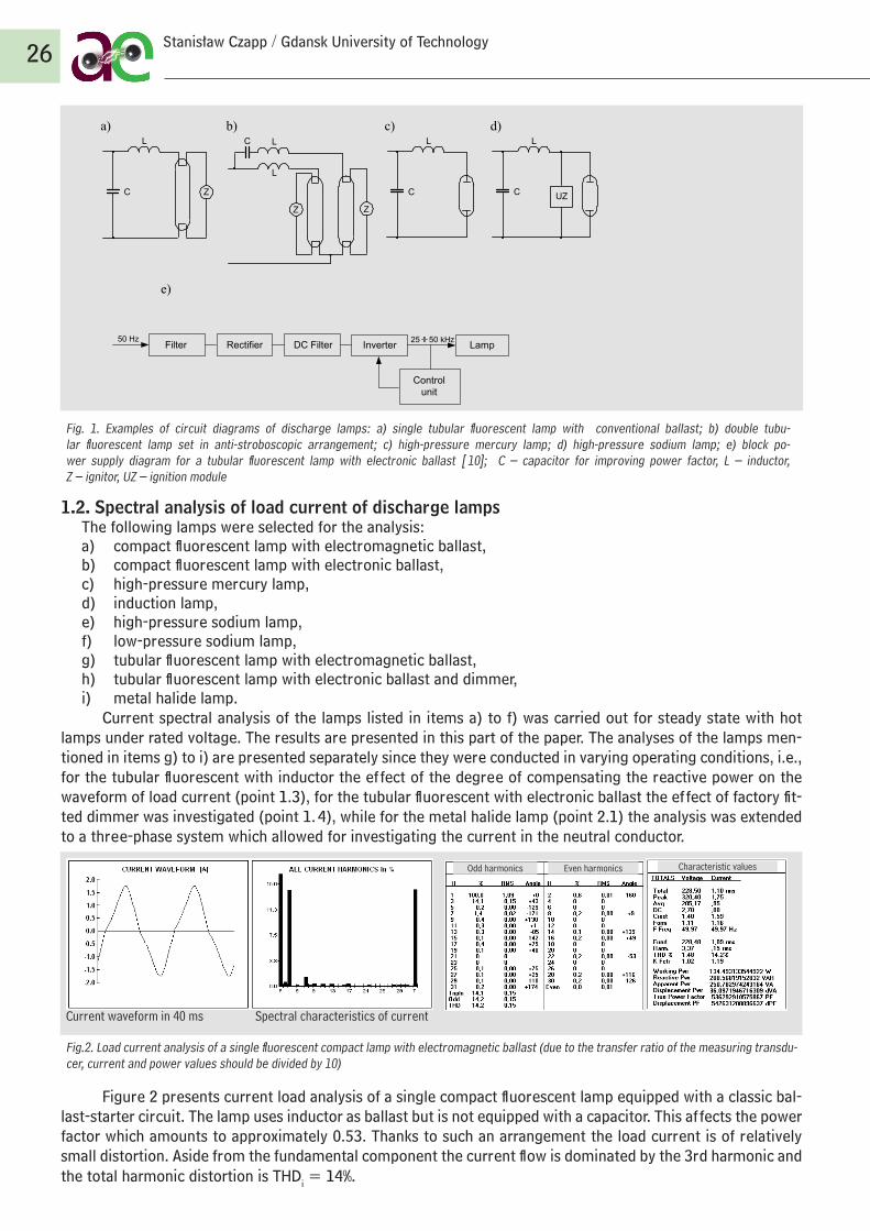
Fig. 1. Examples of circuit diagrams of discharge lamps: a) single tubular fluorescent lamp with conventional ballast; b) double tubu-lar fluorescent lamp set in anti-stroboscopic arrangement; c) high-pressure mercury lamp; d) high-pressure sodium lamp; e) block po-wer supply diagram for a tubular fluorescent lamp with electronic ballast [10]; C – capacitor for improving power factor, L – inductor, Z – ignitor, UZ – ignition module
1.2. Spectral analysis of load current of discharge lampsThe following lamps were selected for the analysis:a) compact fluorescent lamp with electromagnetic ballast,b) compact fluorescent lamp with electronic ballast,c) high-pressure mercury lamp,d) induction lamp,e) high-pressure sodium lamp,f) low-pressure sodium lamp,g) tubular fluorescent lamp with electromagnetic ballast,h) tubular fluorescent lamp with electronic ballast and dimmer,i) metal halide lamp.
Current spectral analysis of the lamps listed in items a) to f) was carried out for steady state with hot lamps under rated voltage. The results are presented in this part of the paper. The analyses of the lamps men-tioned in items g) to i) are presented separately since they were conducted in varying operating conditions, i.e., for the tubular fluorescent with inductor the effect of the degree of compensating the reactive power on the waveform of load current (point 1.3), for the tubular fluorescent with electronic ballast the effect of factory fit-ted dimmer was investigated (point 1. 4), while for the metal halide lamp (point 2.1) the analysis was extended to a three-phase system which allowed for investigating the current in the neutral conductor.
Current waveform in 40 ms Spectral characteristics of current
Fig.2. Load current analysis of a single fluorescent compact lamp with electromagnetic ballast (due to the transfer ratio of the measuring transdu-cer, current and power values should be divided by 10)
Figure 2 presents current load analysis of a single compact fluorescent lamp equipped with a classic bal-last-starter circuit. The lamp uses inductor as ballast but is not equipped with a capacitor. This affects the power factor which amounts to approximately 0.53. Thanks to such an arrangement the load current is of relatively small distortion. Aside from the fundamental component the current flow is dominated by the 3rd harmonic and the total harmonic distortion is THDi = 14%.
26 Stanisław Czapp / Gdansk University of Technology
Characteristic valuesEven harmonicsOdd harmonics
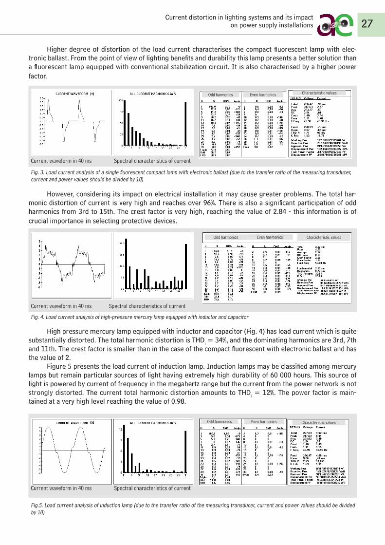
Higher degree of distortion of the load current characterises the compact fluorescent lamp with elec-tronic ballast. From the point of view of lighting benefits and durability this lamp presents a better solution than a fluorescent lamp equipped with conventional stabilization circuit. It is also characterised by a higher power factor.
Current waveform in 40 ms Spectral characteristics of current
Fig. 3. Load current analysis of a single fluorescent compact lamp with electronic ballast (due to the transfer ratio of the measuring transducer, current and power values should be divided by 10)
However, considering its impact on electrical installation it may cause greater problems. The total har-monic distortion of current is very high and reaches over 96%. There is also a significant participation of odd harmonics from 3rd to 15th. The crest factor is very high, reaching the value of 2.84 - this information is of crucial importance in selecting protective devices.
Current waveform in 40 ms Spectral characteristics of current
Fig. 4. Load current analysis of high-pressure mercury lamp equipped with inductor and capacitor
High pressure mercury lamp equipped with inductor and capacitor (Fig. 4) has load current which is quite substantially distorted. The total harmonic distortion is THDi = 34%, and the dominating harmonics are 3rd, 7th and 11th. The crest factor is smaller than in the case of the compact fluorescent with electronic ballast and has the value of 2.
Figure 5 presents the load current of induction lamp. Induction lamps may be classified among mercury lamps but remain particular sources of light having extremely high durability of 60 000 hours. This source of light is powered by current of frequency in the megahertz range but the current from the power network is not strongly distorted. The current total harmonic distortion amounts to THDi = 12%. The power factor is main-tained at a very high level reaching the value of 0.98.
Current waveform in 40 ms Spectral characteristics of current
Fig.5. Load current analysis of induction lamp (due to the transfer ratio of the measuring transducer, current and power values should be divided by 10)
27Current distortion in lighting systems and its impact
on power supply installations
Characteristic valuesEven harmonicsOdd harmonics
Characteristic valuesEven harmonicsOdd harmonics
Characteristic valuesEven harmonicsOdd harmonics
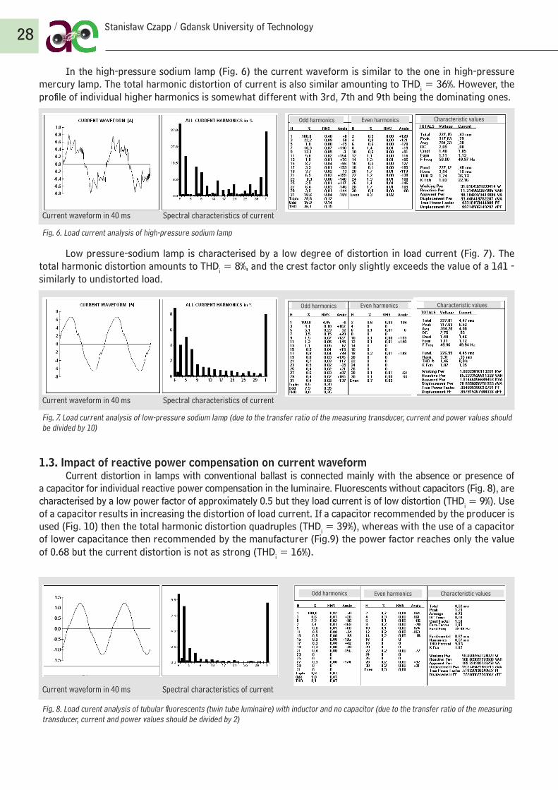
In the high-pressure sodium lamp (Fig. 6) the current waveform is similar to the one in high-pressure mercury lamp. The total harmonic distortion of current is also similar amounting to THDi = 36%. However, the profile of individual higher harmonics is somewhat different with 3rd, 7th and 9th being the dominating ones.
Current waveform in 40 ms Spectral characteristics of current
Fig. 6. Load current analysis of high-pressure sodium lamp
Low pressure-sodium lamp is characterised by a low degree of distortion in load current (Fig. 7). The total harmonic distortion amounts to THDi = 8%, and the crest factor only slightly exceeds the value of a 1.41 - similarly to undistorted load.
Current waveform in 40 ms Spectral characteristics of current
Fig. 7. Load current analysis of low-pressure sodium lamp (due to the transfer ratio of the measuring transducer, current and power values should be divided by 10)
1.3. Impact of reactive power compensation on current waveformCurrent distortion in lamps with conventional ballast is connected mainly with the absence or presence of
a capacitor for individual reactive power compensation in the luminaire. Fluorescents without capacitors (Fig. 8), are characterised by a low power factor of approximately 0.5 but they load current is of low distortion (THDi = 9%). Use of a capacitor results in increasing the distortion of load current. If a capacitor recommended by the producer is used (Fig. 10) then the total harmonic distortion quadruples (THDi = 39%), whereas with the use of a capacitor of lower capacitance then recommended by the manufacturer (Fig.9) the power factor reaches only the value of 0.68 but the current distortion is not as strong (THDi = 16%).
Current waveform in 40 ms Spectral characteristics of current
Fig. 8. Load curent analysis of tubular fluorescents (twin tube luminaire) with inductor and no capacitor (due to the transfer ratio of the measuring transducer, current and power values should be divided by 2)
28 Stanisław Czapp / Gdansk University of Technology
Characteristic valuesEven harmonicsOdd harmonics
Characteristic valuesEven harmonicsOdd harmonics
Characteristic valuesEven harmonicsOdd harmonics
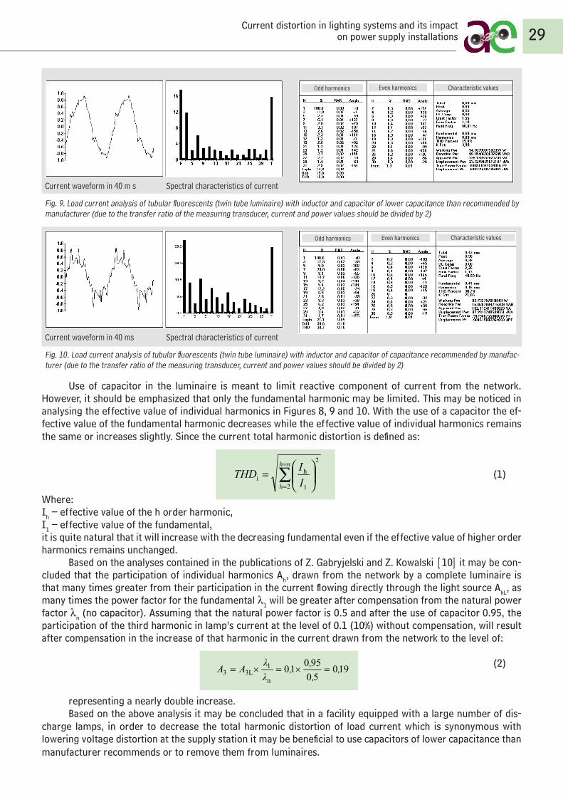
Current waveform in 40 m s Spectral characteristics of current
Fig. 9. Load current analysis of tubular fluorescents (twin tube luminaire) with inductor and capacitor of lower capacitance than recommended by manufacturer (due to the transfer ratio of the measuring transducer, current and power values should be divided by 2)
Current waveform in 40 ms Spectral characteristics of current
Fig. 10. Load current analysis of tubular fluorescents (twin tube luminaire) with inductor and capacitor of capacitance recommended by manufac-turer (due to the transfer ratio of the measuring transducer, current and power values should be divided by 2)
Use of capacitor in the luminaire is meant to limit reactive component of current from the network. However, it should be emphasized that only the fundamental harmonic may be limited. This may be noticed in analysing the effective value of individual harmonics in Figures 8, 9 and 10. With the use of a capacitor the ef-fective value of the fundamental harmonic decreases while the effective value of individual harmonics remains the same or increases slightly. Since the current total harmonic distortion is defined as:
∑
=
=
=
nh
h IITHD
2
2
1
hi (1)
Where:Ih – effective value of the h order harmonic,I1 – effective value of the fundamental,it is quite natural that it will increase with the decreasing fundamental even if the effective value of higher order harmonics remains unchanged.
Based on the analyses contained in the publications of Z. Gabryjelski and Z. Kowalski [10] it may be con-cluded that the participation of individual harmonics Ah, drawn from the network by a complete luminaire is that many times greater from their participation in the current flowing directly through the light source AhL, as many times the power factor for the fundamental λ1 will be greater after compensation from the natural power factor λn (no capacitor). Assuming that the natural power factor is 0.5 and after the use of capacitor 0.95, the participation of the third harmonic in lamp’s current at the level of 0.1 (10%) without compensation, will result after compensation in the increase of that harmonic in the current drawn from the network to the level of:
(2)
representing a nearly double increase.Based on the above analysis it may be concluded that in a facility equipped with a large number of dis-
charge lamps, in order to decrease the total harmonic distortion of load current which is synonymous with lowering voltage distortion at the supply station it may be beneficial to use capacitors of lower capacitance than manufacturer recommends or to remove them from luminaires.
29Current distortion in lighting systems and its impact
on power supply installations
Characteristic values
Characteristic values
Even harmonics
Even harmonics
Odd harmonics
Odd harmonics
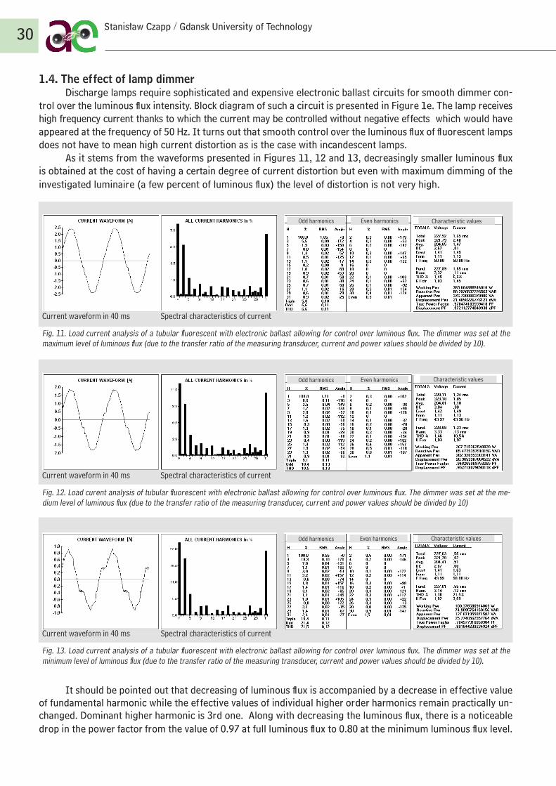
1. 4. The effect of lamp dimmer Discharge lamps require sophisticated and expensive electronic ballast circuits for smooth dimmer con-
trol over the luminous flux intensity. Block diagram of such a circuit is presented in Figure 1e. The lamp receives high frequency current thanks to which the current may be controlled without negative effects which would have appeared at the frequency of 50 Hz. It turns out that smooth control over the luminous flux of fluorescent lamps does not have to mean high current distortion as is the case with incandescent lamps.
As it stems from the waveforms presented in Figures 11, 12 and 13, decreasingly smaller luminous flux is obtained at the cost of having a certain degree of current distortion but even with maximum dimming of the investigated luminaire (a few percent of luminous flux) the level of distortion is not very high.
Current waveform in 40 ms Spectral characteristics of current
Fig. 11. Load current analysis of a tubular fluorescent with electronic ballast allowing for control over luminous flux. The dimmer was set at the maximum level of luminous flux (due to the transfer ratio of the measuring transducer, current and power values should be divided by 10).
Current waveform in 40 ms Spectral characteristics of current
Fig. 12. Load curent analysis of tubular fluorescent with electronic ballast allowing for control over luminous flux. The dimmer was set at the me-dium level of luminous flux (due to the transfer ratio of the measuring transducer, current and power values should be divided by 10)
Current waveform in 40 ms Spectral characteristics of current
Fig. 13. Load current analysis of a tubular fluorescent with electronic ballast allowing for control over luminous flux. The dimmer was set at the minimum level of luminous flux (due to the transfer ratio of the measuring transducer, current and power values should be divided by 10).
It should be pointed out that decreasing of luminous flux is accompanied by a decrease in effective value of fundamental harmonic while the effective values of individual higher order harmonics remain practically un-changed. Dominant higher harmonic is 3rd one. Along with decreasing the luminous flux, there is a noticeable drop in the power factor from the value of 0.97 at full luminous flux to 0.80 at the minimum luminous flux level.
30 Stanisław Czapp / Gdansk University of Technology
Characteristic valuesEven harmonicsOdd harmonics
Characteristic valuesEven harmonicsOdd harmonics
Characteristic valuesEven harmonicsOdd harmonics
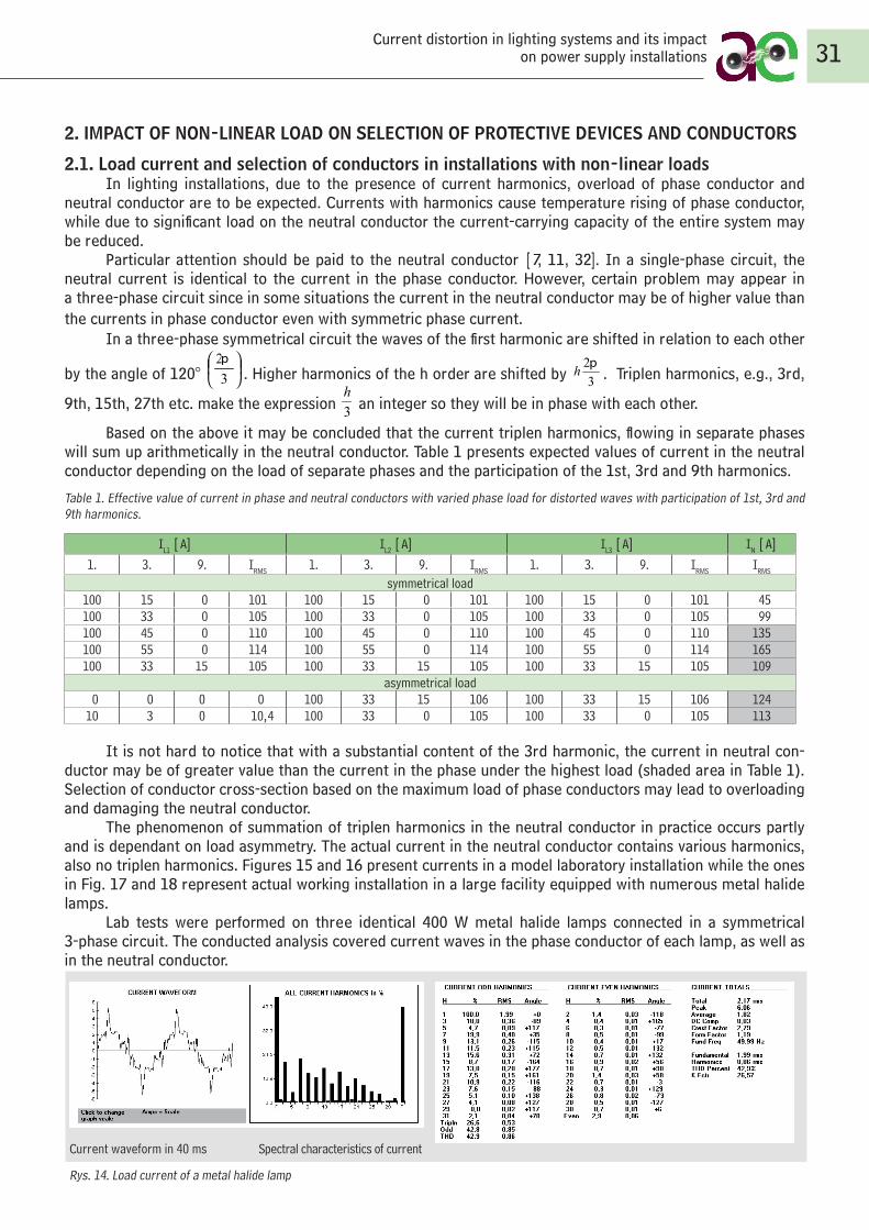
2. IMPACT OF NON-LINEAR LOAD ON SELECTION OF PROTECTIVE DEVICES AND CONDUCTORS
2.1. Load current and selection of conductors in installations with non-linear loadsIn lighting installations, due to the presence of current harmonics, overload of phase conductor and
neutral conductor are to be expected. Currents with harmonics cause temperature rising of phase conductor, while due to significant load on the neutral conductor the current-carrying capacity of the entire system may be reduced.
Particular attention should be paid to the neutral conductor [7, 11, 32]. In a single-phase circuit, the neutral current is identical to the current in the phase conductor. However, certain problem may appear in a three-phase circuit since in some situations the current in the neutral conductor may be of higher value than the currents in phase conductor even with symmetric phase current.
In a three-phase symmetrical circuit the waves of the first harmonic are shifted in relation to each other
by the angle of 120°
32ð
. Higher harmonics of the h order are shifted by 32ph . Triplen harmonics, e.g., 3rd,
9th, 15th, 27th etc. make the expression 3h
an integer so they will be in phase with each other.
Based on the above it may be concluded that the current triplen harmonics, flowing in separate phases will sum up arithmetically in the neutral conductor. Table 1 presents expected values of current in the neutral conductor depending on the load of separate phases and the participation of the 1st, 3rd and 9th harmonics.
Table 1. Effective value of current in phase and neutral conductors with varied phase load for distorted waves with participation of 1st, 3rd and 9th harmonics.
IL1 [A] IL2 [A] IL3 [A] IN [A]
1. 3. 9. IRMS 1. 3. 9. IRMS 1. 3. 9. IRMS IRMS
symmetrical load100 15 0 101 100 15 0 101 100 15 0 101 45100 33 0 105 100 33 0 105 100 33 0 105 99100 45 0 110 100 45 0 110 100 45 0 110 135100 55 0 114 100 55 0 114 100 55 0 114 165100 33 15 105 100 33 15 105 100 33 15 105 109
asymmetrical load 0 0 0 0 100 33 15 106 100 33 15 106 12410 3 0 10, 4 100 33 0 105 100 33 0 105 113
It is not hard to notice that with a substantial content of the 3rd harmonic, the current in neutral con-ductor may be of greater value than the current in the phase under the highest load (shaded area in Table 1). Selection of conductor cross-section based on the maximum load of phase conductors may lead to overloading and damaging the neutral conductor.
The phenomenon of summation of triplen harmonics in the neutral conductor in practice occurs partly and is dependant on load asymmetry. The actual current in the neutral conductor contains various harmonics, also no triplen harmonics. Figures 15 and 16 present currents in a model laboratory installation while the ones in Fig. 17 and 18 represent actual working installation in a large facility equipped with numerous metal halide lamps.
Lab tests were performed on three identical 400 W metal halide lamps connected in a symmetrical 3-phase circuit. The conducted analysis covered current waves in the phase conductor of each lamp, as well as in the neutral conductor.
Current waveform in 40 ms Spectral characteristics of current
Rys. 14. Load current of a metal halide lamp
31Current distortion in lighting systems and its impact
on power supply installations
32ph
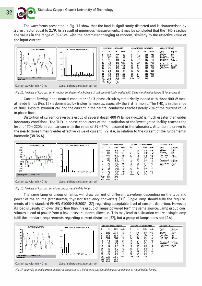
The waveforms presented in Fig. 14 show that the load is significantly distorted and is characterised by a crest factor equal to 2.79. As a result of numerous measurements, it may be concluded that the THDi reaches the values in the range of 39÷54%; with the parameter changing at random, similarly to the effective value of the input current.
Current waveform in 40 ms Spectral characteristics of current
Fig. 15. Analysis of load current in neutral conductor of a 3-phase circuit symmetrically loaded with three metal halide lamps (1 lamp/phase)
Current flowing in the neutral conductor of a 3-phase circuit symmetrically loaded with three 400 W met-al halide lamps (Fig. 15) is dominated by triplen harmonics, especially the 3rd harmonic. The THDi is in the range of 300%. Despite symmetrical load the current in the neutral conductor reaches nearly 70% of the current value in phase lines.
Distortion of current drawn by a group of several dozen 400 W lamps (Fig.16) is much greater than under laboratory conditions. The THDi in phase conductors of the installation of the investigated facility reaches the level of 70÷220%, in comparison with the value of 39÷54% measured in the laboratory. Attention is drawn to the nearly three times greater effective value of current– 92. 4 A, in relation to the current of the fundamental harmonic (38.36 A).
Current waveform in 40 ms Spectral characteristics of current
Fig. 16. Analysis of load current of a group of metal halide lamps
The same lamp or group of lamps will draw current of different waveform depending on the type and power of the source (transformer, thyristor frequency converter) [13]. Single lamp should fulfil the require-ments of the standard PN-EN 61000-3-2:2007 [27] regarding acceptable level of current distortion. However, its load is usually of lower distortion than in a group of lamps powered form the same source. Lamp group con-stitutes a load of power from a few to several dozen kilowatts. This may lead to a situation where a single lamp fulfil the standard requirements regarding current distortion[27], but a group of lamps does not [16].
Current waveform in 40 ms Spectral characteristics of current
Fig. 17. Analysis of load current in neutral conductor of a lighting circuit containing a large number of metal halide lamps.
32 Stanisław Czapp / Gdansk University of Technology

Analysis of current in the neutral conductor of the circuit containing several dozen 400 W metal halide lamps shows (Fig. 17) that the 3rd harmonic is the dominating one. Based on the analysis it may be concluded that current in the neutral conductor has higher value than current in phase conductors even with certain small asymmetry of load. The effective value of this current is over 170 A, while the effective value of the current in phase conductors is approximately 90 A, which is of significance in selecting the cross-section of neutral con-ductor. The neutral conductor cross-section in installations of non-linear loads should not be any smaller than the cross-section of phase conductors
2.2. Selection of overcurrent protective devicesProtection against overloads and short-circuits is provided by circuit breakers and fuses. In selecting
rated current of protective device one should be guided by the effective value of current with providing for cur-rents of higher harmonics. Taking into account higher harmonic currents the effective value of current in phase conductors of a single lamp may be a dozen or so percent higher than in the case of the fundamental harmonic (Fig. 14). The participation of higher harmonics in current may be higher since the combined power of the lamp constitutes significant transformer load.
Discharge lamps are characterised by increased current at the moment of switching on. The transient current value is about 1, 4÷2,01 times greater than rated current value. Data on transient current is provided by lamp manufacturer. Fig. 19 presents changes in current drawn by high-pressure mercury lamp and high-pressure sodium lamp from the point of switching on to reaching steady state [10, 23]. The transient current gradually decreases within a period of few minutes to the rated current value.
Due to the increased current value right after switching the lamp on, the rated current of the circuit breaker should be greater than it might stem from the maximum load current in steady state. In a circuit with discharge lamps with cacapitor, it may be concluded for the sake of simplification that the continuous rated current of the circuit breaker Inw should be high enough not to allow its overload release to react in a given time period to the load current expressed as a multiple of lamp’s rated current Ilam (Tab. 2) [15]. As it stems from Table 2, the rated current of the circuit breaker should be at least 25% greater than the load on the lamp in steady state.
Tabl. 2. Estimated values of transient current and its flow time in circuits of discharge lamps with capacitors
Time ∞ 4 min 2 min
Load current 1,25×Ilam 1,6×Ilam 1,8×Ilam
The changes presented in Fig. 18 apply to the effective value, and as it stems from the oscilograms pre-sented in the previous point, the load current may be strongly distorted. Study results presented in the publica-tion of M. Walejewski [34] show that the current right after switching the lamp on may be of higher distortion than in its steady state. In protective devices selection it is also important whether the current waveform is characterised by high crest factor. Electromagnetic release of the circuit breaker reacts to the peak load value and in order to avoid nuisance tripping the peak current value of non-tripping current of the circuit breaker should be greater than the instantaneous value of the current imax present in all foreseen transient state [22].
Fig. 18. Changes of current load for high-pressure mercury and sodium lamps from ignition to steady state[10, 23];In – current load in steady state
1 Peak value of current at switching on of a lamp equipped with parallel capacitor may amount to several dozen amperes but the pulse will be of very short duration (hundreds of microseconds). Such phenomena is not considered in this paper.
33Current distortion in lighting systems and its impact
on power supply installations
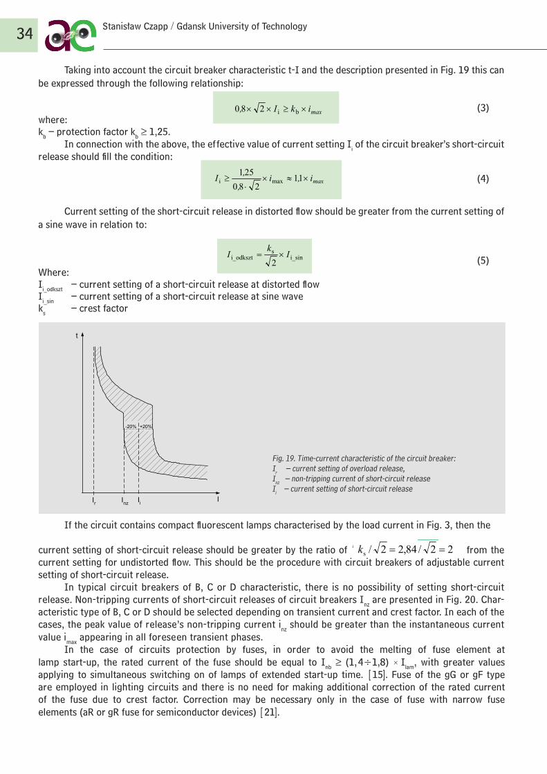
Taking into account the circuit breaker characteristic t-I and the description presented in Fig. 19 this can be expressed through the following relationship:
maxbi28,0 ikI ⋅≥⋅⋅
(3)where:kb – protection factor kb ≥ 1,25.
In connection with the above, the effective value of current setting Ii of the circuit breaker’s short-circuit release should fill the condition:
maxmaxi 1,1
28,025,1 iiI ⋅≈⋅⋅
≥ (4)
Current setting of the short-circuit release in distorted flow should be greater from the current setting of a sine wave in relation to:
i_sin
si_odkszt 2
IkI ⋅= (5)Where:Ii_odkszt – current setting of a short-circuit release at distorted flowIi_sin – current setting of a short-circuit release at sine waveks – crest factor
t
I
-20% +20%
IiIr Inz
Fig. 19. Time-current characteristic of the circuit breaker:Ir – current setting of overload release,Inz – non-tripping current of short-circuit release Ii – current setting of short-circuit release
If the circuit contains compact fluorescent lamps characterised by the load current in Fig. 3, then the
current setting of short-circuit release should be greater by the ratio of 22/84.22/s ==k from the current setting for undistorted flow. This should be the procedure with circuit breakers of adjustable current setting of short-circuit release.
In typical circuit breakers of B, C or D characteristic, there is no possibility of setting short-circuit release. Non-tripping currents of short-circuit releases of circuit breakers Inz are presented in Fig. 20. Char-acteristic type of B, C or D should be selected depending on transient current and crest factor. In each of the cases, the peak value of release’s non-tripping current inz should be greater than the instantaneous current value imax appearing in all foreseen transient phases.
In the case of circuits protection by fuses, in order to avoid the melting of fuse element at lamp start-up, the rated current of the fuse should be equal to Inb ≥ (1, 4÷1,8) × Ilam, with greater values applying to simultaneous switching on of lamps of extended start-up time. [15]. Fuse of the gG or gF type are employed in lighting circuits and there is no need for making additional correction of the rated current of the fuse due to crest factor. Correction may be necessary only in the case of fuse with narrow fuse elements (aR or gR fuse for semiconductor devices) [21].
34 Stanisław Czapp / Gdansk University of Technology
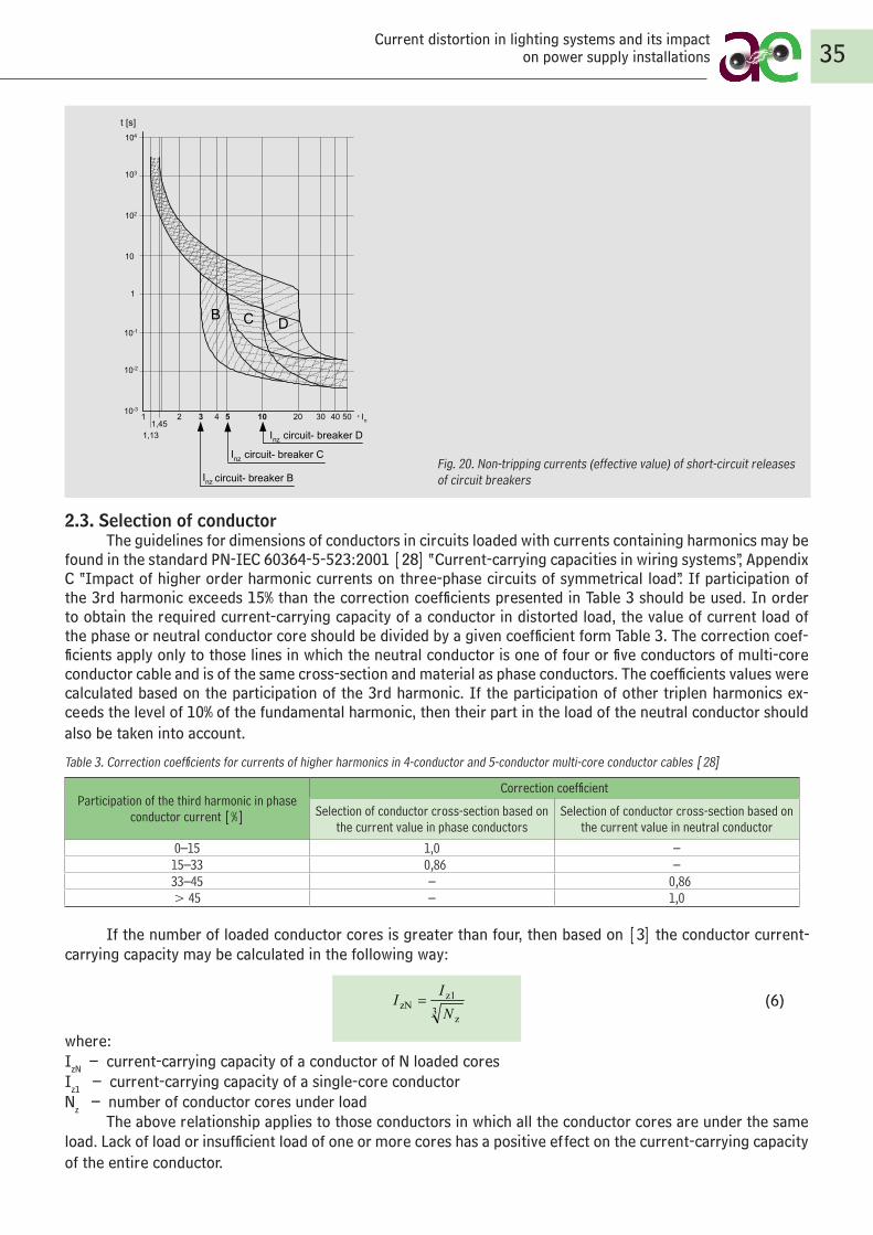
Fig. 20. Non-tripping currents (effective value) of short-circuit releases of circuit breakers
2.3. Selection of conductorThe guidelines for dimensions of conductors in circuits loaded with currents containing harmonics may be
found in the standard PN-IEC 60364-5-523:2001 [28] “Current-carrying capacities in wiring systems”, Appendix C “Impact of higher order harmonic currents on three-phase circuits of symmetrical load”. If participation of the 3rd harmonic exceeds 15% than the correction coefficients presented in Table 3 should be used. In order to obtain the required current-carrying capacity of a conductor in distorted load, the value of current load of the phase or neutral conductor core should be divided by a given coefficient form Table 3. The correction coef-ficients apply only to those lines in which the neutral conductor is one of four or five conductors of multi-core conductor cable and is of the same cross-section and material as phase conductors. The coefficients values were calculated based on the participation of the 3rd harmonic. If the participation of other triplen harmonics ex-ceeds the level of 10% of the fundamental harmonic, then their part in the load of the neutral conductor should also be taken into account.
Table 3. Correction coefficients for currents of higher harmonics in 4-conductor and 5-conductor multi-core conductor cables [28]
Participation of the third harmonic in phase conductor current [%]
Correction coefficient
Selection of conductor cross-section based on the current value in phase conductors
Selection of conductor cross-section based on the current value in neutral conductor
0–15 1,0 –15–33 0,86 –33–45 – 0,86> 45 – 1,0
If the number of loaded conductor cores is greater than four, then based on [3] the conductor current-carrying capacity may be calculated in the following way:
(6)
where:IzN – current-carrying capacity of a conductor of N loaded coresIz1 – current-carrying capacity of a single-core conductorNz – number of conductor cores under load
The above relationship applies to those conductors in which all the conductor cores are under the same load. Lack of load or insufficient load of one or more cores has a positive effect on the current-carrying capacity of the entire conductor.
35Current distortion in lighting systems and its impact
on power supply installations
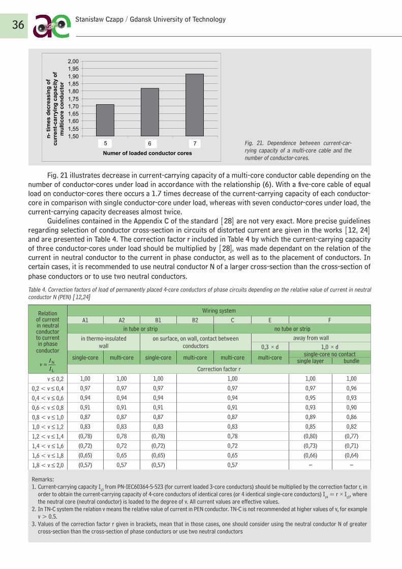
1,501,551,601,651,701,751,801,851,901,952,00
1 2 3
L iczba obciążonych żył
n-kr
otne
zm
niej
szen
ie
obci
ążal
nośc
i prz
ewod
u w
ielo
żyło
weg
o
5 6 7
Fig. 21 illustrates decrease in current-carrying capacity of a multi-core conductor cable depending on the number of conductor-cores under load in accordance with the relationship (6). With a five-core cable of equal load on conductor-cores there occurs a 1.7 times decrease of the current-carrying capacity of each conductor-core in comparison with single conductor-core under load, whereas with seven conductor-cores under load, the current-carrying capacity decreases almost twice.
Guidelines contained in the Appendix C of the standard [28] are not very exact. More precise guidelines regarding selection of conductor cross-section in circuits of distorted current are given in the works [12, 24]and are presented in Table 4. The correction factor r included in Table 4 by which the current-carrying capacity of three conductor-cores under load should be multiplied by [28], was made dependant on the relation of the current in neutral conductor to the current in phase conductor, as well as to the placement of conductors. In certain cases, it is recommended to use neutral conductor N of a larger cross-section than the cross-section of phase conductors or to use two neutral conductors.
Table 4. Correction factors of load of permanently placed 4-core conductors of phase circuits depending on the relative value of current in neutral conductor N (PEN) [12,24]
Relation of current in neutral conductor to current in phase
conductor
L
N
II
v =
Wiring system
A1 A2 B1 B2 C E Fin tube or strip no tube or strip
in thermo-insulated wall
on surface, on wall, contact between conductors
away from wall0,3 × d 1,0 × d
single-core multi-core single-core multi-core multi-core multi-core single-core no contactsingle layer bundle
Correction factor r
v ≤ 0,2 1,00 1,00 1,00 1,00 1,00 1,00
0,2 < v ≤ 0, 4 0,97 0,97 0,97 0,97 0,97 0,96
0, 4 < v ≤ 0,6 0,94 0,94 0,94 0,94 0,95 0,93
0,6 < v ≤ 0,8 0,91 0,91 0,91 0,91 0,93 0,90
0,8 < v ≤ 1,0 0,87 0,87 0,87 0,87 0,89 0,86
1,0 < v ≤ 1,2 0,83 0,83 0,83 0,83 0,85 0,82
1,2 < v ≤ 1, 4 (0,78) 0,78 (0,78) 0,78 (0,80) (0,77)
1, 4 < v ≤ 1,6 (0,72) 0,72 (0,72) 0,72 (0,73) (0,71)
1,6 < v ≤ 1,8 (0,65) 0,65 (0,65) 0,65 (0,66) (0,64)
1,8 < v ≤ 2,0 (0,57) 0,57 (0,57) 0,57 – –
Remarks: 1. Current-carrying capacity Iz3 from PN-IEC60364-5-523 (for current loaded 3-core conductors) should be multiplied by the correction factor r, in
order to obtain the current-carrying capacity of 4-core conductors of identical cores (or 4 identical single-core conductors) Iz4 = r × Iz3, where the neutral core (neutral conductor) is loaded to the degree of v. All current values are effective values.
2. In TN-C system the relation v means the relative value of current in PEN conductor. TN-C is not recommended at higher values of v, for example v > 0.5.
3. Values of the correction factor r given in brackets, mean that in those cases, one should consider using the neutral conductor N of greater cross-section than the cross-section of phase conductors or use two neutral conductors
36 Stanisław Czapp / Gdansk University of Technology
Fig. 21. Dependence between current-car-rying capacity of a multi-core cable and the number of conductor-cores.
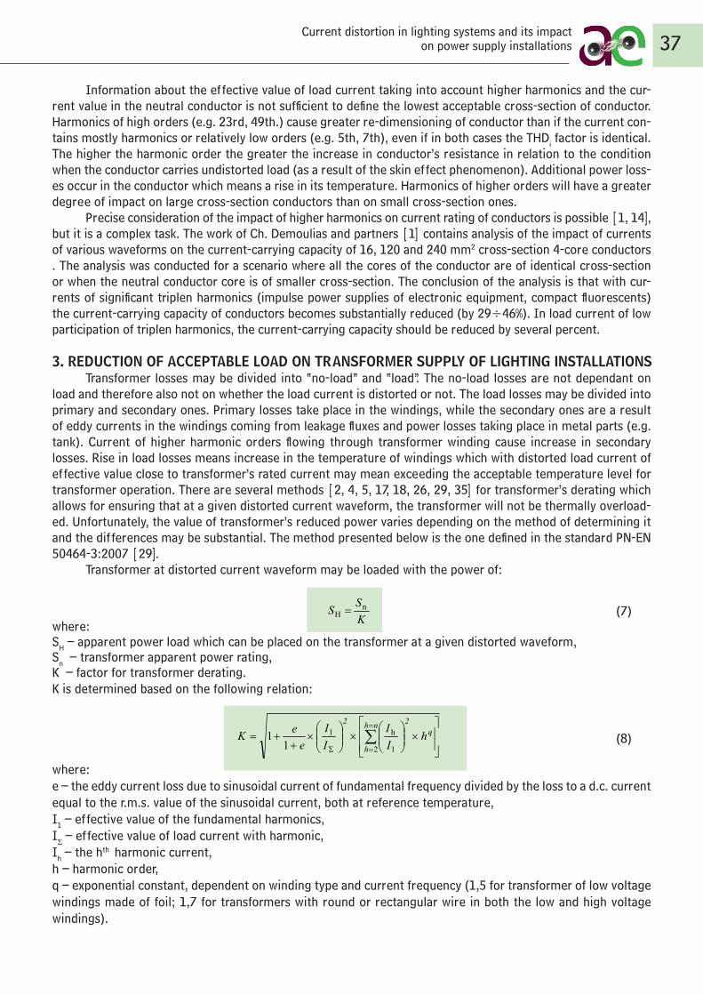
Information about the effective value of load current taking into account higher harmonics and the cur-rent value in the neutral conductor is not sufficient to define the lowest acceptable cross-section of conductor. Harmonics of high orders (e.g. 23rd, 49th.) cause greater re-dimensioning of conductor than if the current con-tains mostly harmonics or relatively low orders (e.g. 5th, 7th), even if in both cases the THDi factor is identical. The higher the harmonic order the greater the increase in conductor’s resistance in relation to the condition when the conductor carries undistorted load (as a result of the skin effect phenomenon). Additional power loss-es occur in the conductor which means a rise in its temperature. Harmonics of higher orders will have a greater degree of impact on large cross-section conductors than on small cross-section ones.
Precise consideration of the impact of higher harmonics on current rating of conductors is possible [1, 14], but it is a complex task. The work of Ch. Demoulias and partners [1] contains analysis of the impact of currents of various waveforms on the current-carrying capacity of 16, 120 and 240 mm2 cross-section 4-core conductors . The analysis was conducted for a scenario where all the cores of the conductor are of identical cross-section or when the neutral conductor core is of smaller cross-section. The conclusion of the analysis is that with cur-rents of significant triplen harmonics (impulse power supplies of electronic equipment, compact fluorescents) the current-carrying capacity of conductors becomes substantially reduced (by 29÷46%). In load current of low participation of triplen harmonics, the current-carrying capacity should be reduced by several percent.
3. REDUCTION OF ACCEPTABLE LOAD ON TRANSFORMER SUPPLY OF LIGHTING INSTALLATIONS Transformer losses may be divided into “no-load” and “load”. The no-load losses are not dependant on
load and therefore also not on whether the load current is distorted or not. The load losses may be divided into primary and secondary ones. Primary losses take place in the windings, while the secondary ones are a result of eddy currents in the windings coming from leakage fluxes and power losses taking place in metal parts (e.g. tank). Current of higher harmonic orders flowing through transformer winding cause increase in secondary losses. Rise in load losses means increase in the temperature of windings which with distorted load current of effective value close to transformer’s rated current may mean exceeding the acceptable temperature level for transformer operation. There are several methods [2, 4, 5, 17, 18, 26, 29, 35] for transformer’s derating which allows for ensuring that at a given distorted current waveform, the transformer will not be thermally overload-ed. Unfortunately, the value of transformer’s reduced power varies depending on the method of determining it and the differences may be substantial. The method presented below is the one defined in the standard PN-EN 50464-3:2007 [29].
Transformer at distorted current waveform may be loaded with the power of:
KSS n
H = (7)where:SH – apparent power load which can be placed on the transformer at a given distorted waveform,Sn – transformer apparent power rating,K – factor for transformer derating.K is determined based on the following relation:
⋅
⋅
⋅
++= ∑
=
=
nh
2h
q22
hII
II
eeK
1
h
Ó
1
11 (8)
where:e – the eddy current loss due to sinusoidal current of fundamental frequency divided by the loss to a d.c. current equal to the r.m.s. value of the sinusoidal current, both at reference temperature,I1 – effective value of the fundamental harmonics,IΣ – effective value of load current with harmonic,Ih – the hth harmonic current,h – harmonic order,q – exponential constant, dependent on winding type and current frequency (1,5 for transformer of low voltage windings made of foil; 1,7 for transformers with round or rectangular wire in both the low and high voltage windings).
37Current distortion in lighting systems and its impact
on power supply installations
If a 630 kVA rated power transformer was loaded with current of the waveform presented in Fig.15 (pow-ering a single lamp under lab conditions), then following power could be drawn from it for long duration:
(9)
so its use would be limited to the level of 81% (assuming e = 0.05 and q = 1.7). In a facility with a large number of lamps which constitute the dominant transformer load, current distortions are greater than under laboratory conditions (Fig. 17) and are difficult to predetermine [20]. With such current waveform, the power which can be provided by the transformer is even smaller and equals 440 kVA (0.7×Sn).
4. CONCLUSIONSDistortion of load current in lighting systems depends on the type of installed light source and the ballast-
ignition circuit, as well as the power source rating. The impact of current distortion should be taken into consid-eration in selecting protective devices, conductors and power transformer. Therefore, it is advisable to examine quite closely the properties of lighting devices, which are to be included in the installation, especially in the area regarding the participation of harmonics in the load current. This is particularly important when the devices are to constitute a substantial participation in facility’s combined power demand and transformer’s load.
LITERATURE
1. Demoulias Ch., Labridis D.P., Dokopoulos S.P., Gouramanis K., Ampacity of Low-Voltage Power Cables Under Nonsi-nusoudal Currents. IEEE Transactions on Power Delivery, 2007, vol. 22, no. 1, s. 584–594.
2. Desmet J., Lemcko L., Harmoniczne. Dopuszczalna obciążalność i dobór transformatorów do pracy z prądem od-kształconym. Leonardo Power Quality Initiative. Jakość zasilania – poradnik, cz. 3.5.2, listopad 2005.
3. Det Norske Veritas. Rules for classification of ships. Part 4 – Machinery and Systems – Main Class. Chapter 4 – Elec-trical Installations. Edition 1999.
4. Faiz J., Sharifian M.B.B., Fakheri S.A., Sabet-Marzooghi E., Derating of Distribution Transformers for Non-sinusoidal Load Currents Using Finite Element Method. Iranian Journal of Science & Technology, Transaction B, 2004, vol. 28, no. B3, s. 315–322.
5. Filtracja i detekcja harmonicznych. Schneider Electric. Materiały firmowe.6. Gabryjelski Z., Świetlówki kompaktowe jako źródło zaburzeń elektromagnetycznych. Przegląd Elektrotechniczny,
2007, nr 9, s. 100–103.7. Gabryjelski Z., Praca świetlówek kompaktowych w sieci trójfazowej. Przegląd Elektrotechniczny, 2007, nr 9, s. 42–43.8. Gabryjelski Z., Odkształcenie prądu w obwodach lamp fluorescencyjnych i wyładowczych połączonych ze stateczni-
kiem indukcyjnym. Archiwum Elektrotechniki, 1982, t. XXXI, z. 1–2, s. 125–136.9. Gabryjelski Z., Odkształcenie prądu w obwodach lamp fluorescencyjnych i wyładowczych połączonych ze stateczni-
kiem pojemnościowo-indukcyjnym. Archiwum Elektrotechniki, 1982, t. XXXI, z. 3-4, s. 571–581.10. Gabryjelski Z., Kowalski Z.: Sieci i urządzenia oświetleniowe. Zagadnienia wybrane. Politechnika Łódzka. Łódź 1997.11. Gabryjelski Z., Kowalski Z.: Przyczyny obciążania przewodów zerowych w sieciach oświetleniowych. Gospodarka
Paliwami i Energią, 1977, nr 7, s. 21–23.12. Hering E., Leitungen mit vier belasteten Leitern. Elektropraktiker, 2004, nr 9, s. 722–726.13. Herlender K., Cadler E.: Wpływ sposobu zasilania nowoczesnych układów oświetleniowych na jakość energii elek-
trycznej. Wiadomości Elektrotechniczne, 2006, nr 3, s. 30–32.14. Hiranandani A.: Calculation of Cable Ampacities Including the Effect of Harmonics. IEEE Industry Applications
Magazine, March/April 1998, s. 42–51. 15. Instalacje elektryczne i teletechniczne. Poradnik montera i inżyniera elektryka. Verlag Dashöfer. Część 5. Zabezpie-
czenia w instalacjach elektrycznych.16. Kasprzak A., Orlikowski M., Brodecki D., O pewnych aspektach EMC dotyczących powszechnego wprowadzenia
świetlówek energooszczędnych. Przegląd Elektrotechniczny, 2007, nr 9, s. 104–105.17. Kelley A.W., Edwards S.W., Rhode J.P. Baran M.E., Transformer Derating for Harmonic Currents: A Wide-Band Mea-
surement Approach for Energized Transformers. IEEE Transactions on Industry Applications, 1999, vol. 35, no. 6, s. 1450–1457.
18. Kuśmierek Z., Współczynnik obciążenia transformatora zasilającego odbiorniki nieliniowe i jego pomiar. Przegląd Elektrotechniczny, 2004, nr 6, s. 636–638.
19. Magdziak R. Układy zabezpieczeń w elektronicznych statecznikach świetlówek. Elektronizacja, 2000, nr 4, s. 18–19.
38 Stanisław Czapp / Gdansk University of Technology

20. Musiał E., Czapp S., Opinia w sprawie zakłóceń wywołanych prądami wyższych harmonicznych w instalacji elek-trycznej supermarketu OBI w Gdyni-Cisowej. Gdańsk 1999.
21. Musiał E., Bezpieczniki w nowoczesnych układach zabezpieczeń urządzeń niskiego napięcia. Ogólnopolskie Szkole-nie Techniczne „Zabezpieczenia niskonapięciowych instalacji i urządzeń elektrycznych”. ENERGO-EKO-TECH, Poznań, paź-dziernik 2001.
22. Musiał E., Zabezpieczanie silników zasilanych z pośrednich przemienników częstotliwości. INPE Informacje o Nor-mach i Przepisach Elektrycznych, Miesięcznik SEP, 2004, nr 59–60, s. 3–35.
23. Musiał E., Przegląd elektrycznych źródeł światła. Główne właściwości i tendencje rozwojowe. INPE Informacje o Normach i Przepisach Elektrycznych, Miesięcznik SEP, 2006, nr 79, s. 3–66.
24. Musiał E., Obciążalność cieplna oraz zabezpieczenia nadprądowe przewodów i kabli. INPE Informacje o Normach i Przepisach Elektrycznych, Miesięcznik SEP, 2008, nr 107, s. 3–41.
25. Pabjańczyk W., Oszczędności energetyczne wynikające ze stosowania elektronicznych urządzeń stabilizacyjno-za-płonowych. Wiadomości Elektrotechniczne, 2000, nr 10, s. 540–543.
26. Pierce L.W., Transformer Design and Application Considerations for Nonsinusoidal Load Currents, IEEE Transactions on Industry Applications, 1996, vol. 32, no. 3, s. 633–645.
27 PN-EN 61000-3-2:2007 Kompatybilność elektromagnetyczna (EMC). Część 3-2: Poziomy dopuszczalne. Poziomy dopuszczalne emisji harmonicznych prądu (fazowy prąd zasilający odbiornika < lub = 16 A).
28. PN-IEC 60364-5-523:2001 Instalacje elektryczne w obiektach budowlanych. Dobór i montaż wyposażenia elek-trycznego. Obciążalność prądowa długotrwała przewodów.
29. PN-EN 50464-3:2007 Trójfazowe olejowe transformatory rozdzielcze 50 Hz od 50 kVA do 2500 kVA o najwyższym napięciu urządzenia nie przekraczającym 36 kV. Część 3: Wyznaczanie mocy znamionowej transformatora obciążonego prądem niesinusoidalnym. (oryg.)
30. Różowicz A., Systemy świetlne jako źródło zakłóceń. Przegląd Elektrotechniczny, 2003, nr 4, s. 296–299.31. Różowicz A., Skuteczność świetlna lamp fluorescencyjnych zasilanych prądem o różnej częstotliwości. Wiadomości
Elektrotechniczne, 2004, nr 11, s. 15–18.32. Rydzewski Z., Nowosielski J., Specyficzne cechy świetlówek jako odbiorników sieci trójfazowej niskiego napięcia.
Przegląd Elektrotechniczny, 1973, nr 7, s. 331–335.33. Starzak Ł., Bek S., Modelowanie kompaktowych lamp fluorescencyjnych do badań ich oddziaływania na sieć zasila-
jącą. Przegląd Elektrotechniczny, 2007, nr 9, s. 106–107.34. Walejewski M., Analiza jakości energii elektrycznej w instalacjach oświetleniowych. Praca dyplomowa magisterska.
Politechnika Gdańska, Gdańsk 2006. 35. Yildirim D., Fuchs E.F., Measured Transformer Derating and Comparision with Harmonic Loss Factor (FHL) Approach.
IEEE Transactions on Power Delivery, 2000, vol. 15, no. 1, s. 186–191.
39Current distortion in lighting systems and its impact
on power supply installations

Author / Biographie
Andrzej GraczykWrocław / Poland
Head of the Environmental Economy Chair at the Wrocław University of Economics in Wrocław. Graduate of the National Economy Faculty of the Wrocław University of Economics, MA degree in 1978, Ph.D. - in 1988, habilitacja [second level doctorate] in 2005. In the years 1999–2005 De-puty Dean for Didactics at the Faculty of National Economy and starting 2005 Dean of the Faculty of Economic Sciences at the Wrocław University of Economics in Wrocław. Research areas related to environmental eco-nomics and environmental management, power management, theory and practice in sustainable development. In the years 2003–2004 he was the head of the team for financial and economic environmental development mechanisms of the Expert Council appointed by the Minister of the Environment. He is a member of the Scienti-fic and Technical Council of Energa Group and Programme Council for Application of Advanced Technologies CATA.
40Andrzej Graczyk / Wrocław University of Economics

DEVELOPMENT OF CO2 EMISSION TRADING IN THE EUROPEAN UNION1
Andrzej Graczyk / Wrocław University of Economics
THE CONCEPT OF EMISSION TRADING Tradable emission allowances/credits are a relatively new instrument for regulating pollution emissions
(and emission reduction rate). The concept at its initial stage involved resignation from controlling the quality of the environment with norms and standards set for emitters. An agency (office) responsible for environmental control was to decide on the admissible or tolerable pollution load and the relevant number of emission allow-ances and next introduce them to the market, distributing them free of charge or selling the credits to emitters.
The key element of the concept is the allowance/credit, which the emitters can sell and buy on the cre-ated secondary market. The demand for credits is created by allowance holders who may refrain from exercis-ing the right to emit a specified quantity of pollutants, but to sell this right to another entity. Allowances may then be further sold and bought on the emission credits market. The motive underlying the transactions is the benefit enjoyed by the parties involved and the choice of the cheapest way of compliance with environmental regulations.
Emitters whose costs of reducing emissions below the assigned limit are lower may lower their emission levels and sell extra emission rights to other emitters (with higher emission costs). For the latter the purchase of additional emission credits is more profitable than emission reduction. Trading will continue until the differ-ences of marginal costs of emission reduction disappear. The credits market will reach equilibrium when the price is equal to marginal costs of all emission sources. Thus, emission trading will automatically satisfy the conditions for minimising social costs of reaching the specified environmental quality level. The projected emis-sion reduction will be performed by those who can reach the target at the lowest cost.
The emission credits market may – if it is properly designed – lead to a major drop of environmental pro-tection costs of society in general, particularly as compared with an administrative regulating system, (emission standards). Tradable emission rights would be exercised wherever they are cheaper than the required measures reducing emissions. And on the contrary, they would not be applied should the drop of emission levels require smaller outlays than the purchase of relevant emission allowances. This means that any admissible pollution load for the environment could be attainable in this system at minimum overall social cost.
The emission credits market may – if it is properly designed – lead to a major drop of environmental pro-tection costs of society in general, particularly as compared with an administrative regulating system, (emission standards). Tradable emission rights would be exercised wherever they are cheaper than the required measures
1 Research project financed from the state budget for science in the years 2007–2009.
The article presents the concept of emission credits trading. The development of the market for emission trading in the European Union resulted from the lack of progress in ratifying the Kyoto Protocol, which was to open a global market. Several stages can be identified in the development of the European system for emission trading. The years 1997–2004 were devoted to preparing the political, concep-tual and regulatory grounds for market development. The first stage, in the years 2005–2007, was a trial period, where emission allowances for voluntary participants were alloca-ted at no cost by particular countries according to criteria set out on the basis of historical emissions.
The second stage of implementing the emission tra-ding system (2008–2012) overlaps with the first period of Kyoto protocol commitments where the allowance alloca-
tion method was uniform in all EU States. The participation of entities in identified sectors is mandatory. The distribution of tradable credits is free of charge but continuous to be based on historical emission data. A secondary emission cre-dit market is developing. In the third period – in the years 2013–2020 – the range of market players will grow. Sys-tematic development of the auction system for allowance distribution will follow. The development of the system for emission trading after 2020 will depend on the adoption of an international agreement on reducing emissions globally.
The article is to present the development of the Eu-ropean Union market, which is the leader of applying market mechanisms to protect the climate.
Abstract
Development of CO2 emission trading in the european union41

reducing emissions. And on the contrary, they would not be applied should the drop of emission levels require smaller outlays than the purchase of relevant emission allowances. This means that any admissible pollution load for the environment could be attainable in this system at minimum overall social cost.
FLEXIBLE MECHANISMS UNDER THE KYOTO PROTOCOLIntroduction of new market solutions in limiting emission of greenhouse gases are connected with the
Protocol to the United Nations Framework Convention on climatic changes adopted in Kyoto on 11 December 1997, further referred to as the Kyoto Protocol2. On 16 February 2005, the Kyoto Protocol came into force rati-fied by 55 countries in Annex 1, who in total emit at least 55% of the global CO2 emission as of 1990.
The Kyoto Protocol introduced several mechanisms facilitating performance of commitments on emis-sion reduction by exchange of the so-called reduction units between countries – Convention parties. The most important instruments for such cooperation are:
• The Joint Implementation Mechanism – JI where the Emission Reduction Unit – ERU is obtained in joint implementation projects;
• Clean Development Mechanism – CDM, where trade covers units of Certified Emission Reduction (CER); • Emission Trading Mechanism – ET, according to which Assigned Amount Units – AAU are traded.
The primary aim of introducing market mechanisms, called flexible mechanisms, is the drive to reduce costs of implementing reduction objectives under the Kyoto Protocol. The mechanisms allow for the achieve-ment of targeted emission reduction of these gasses on a global scale by trading CRU and ERU between parties to the Convention. At the same time, this new form of activating international cooperation has a considerable development potential.
The solutions were adopted for a limited time period, up to the year 2012. Nevertheless, the European Union drives at concluding a new international agreement that will be binding after the year 2012. Therefore, we can expect that the mechanisms applied to that date will also function later.
PREPARATORY MEASURES FOR CREATING A EUROPEAN MARKET FOR EMISSION CREDITS - 1997–2004
At the beginning of the nineties tradable allowances were deemed to be a controversial solution in many European countries. Emission trading was exercised on a limited scale, often as an experiment3. Proposals of introducing an international system for emission trading in greenhouse gasses appeared at the stage of prepar-ing for the conference in Kyoto (1997).
As there was no option for immediate introduction of the Protocol worldwide4, European Union States initiated action towards introducing emission trade within the Community. In 2000 work on emission trade gained impetus. The European Commission in March of that year published the “Green Paper on greenhouse gas emissions trading within the European Union”, and in November of the same year the European Parliament committed the Commission to prepare the emission trading scheme by the year 2005. In October 2001, Com-mission Communication from Goteborg for the European Council “A Sustainable Europe for a Better World: a European Union Strategy for Sustainable Development” confirmed the need to develop a European scheme for carbon dioxide emission trading.
The Kyoto protocol was approved by the Council Decisions 2002/358/EC of 25 April 2002. The Commu-nity and its Member States agreed to jointly comply with the commitment to reduce anthropogenic greenhouse gasses according to the Kyoto Protocol. In the above period two EU countries implemented their own internal systems for emission trading – Denmark in 1999 (mandatory participations of the energy sector) and Great Brit-ain in 2002 (voluntary participation for enterprises from all sectors). Additionally in third countries – Sweden, The Netherlands and Germany widespread research was carried out on the option of implementing tradable allowances, whereas France developed a scheme for voluntary agreements regarding reduction of greenhouse emissions which may evolve into emission trading.
The sixth Community Programme5 specified reduction of greenhouse emissions as one of four priorities
2 Journal of Laws no 203, item 1684, of 17 October 2005.3 These examples are given in the book by: Fiedor B., Graczyk A., Jakubczyk Z., Rynek pozwoleń na emisję zanieczyszczeń na przykładzie SO2 w energetyce polskiej, Wydawnictwo Ekonomia i Środowisko, Białystok 2002, pp. 39–42.4 On 16 February 2005 the Kyoto Protocol came into force ratified by 55 countries, according to Annex I to the Protocol, that in total emitted at least 55% of CO2 in global terms in 1990.5 Established by the European Parliament and European Council Decision No 1600/2002/EC (Official Journal L 242 dated 10.9.2002, p. 1).
42Andrzej Graczyk / Wrocław University of Economics

in environmental sphere. The programme agrees that the Community is involved in reaching an 8 % reduction of greenhouse emission from 2008 to 2012 compared to 1990, and in the long term perspective global green-house emissions will have to be reduced by approximately 70% as compared to 1990. In connection with the above programme a European Parliament and European Council Directive was drafted on a system for trading GHG credits in the Community and to amend Directive 96/61/EC6.
Directive 2003/87/EC7 was adopted in October 2003 with the aim of improving successful compliance with the commitment of the European Community and its Member States by effective European trade in GHG emission allowances with the least detrimental impact on economic development and employment8. It obliged EU Member States to establish national systems for GHG emission trading. The Directive stipulated that the system will be mandatory in all Community countries starting 2005. It projected limited trading in the Com-munity as early as in 2005 in order to facilitate development of relevant strategies before open emission trade under the Kyoto Protocol in 2008.
THE FIRST STAGE OF MARKET DEVELOPMENT 2005–2007The system for emission trading was introduced in two stages. The first stage (in the years 2005–2007)
was a trial period, where emission limits for traders were allocated at no cost by particular countries according to criteria set out in the Directive on the basis of historical emissions (i.e. grandfathering method). Member States divided emission credits for 2298.5 million Mg of carbon dioxide with nearly 95% free of charge.
The system covered emission of carbon dioxide generated by various heat and power plants with high emission levels and other power consuming industrial sectors, such as: incineration plants, oil refineries, coke plants, steel mills, cement factories, brick factories, glass mills, plants producing lime, ceramics, pulp and paper.
The National Emissions Trading Schemes for the years 2005–2007 covered only one (CO2) of the green-house gasses and only part of the domestic emission. Due to the above, it was impossible to apply the Kyoto Protocol objectives as emission limits in the ETS. Nevertheless, Annex III to Directive 2003/87/EC required for the total number of allowances granted under ETS before 2008 to be in line with the drive to satisfy the Kyoto Protocol requirements.
A significant change in the system also included a change in the procedures tor issuing emission allow-ances. Directive 96/61/EC was amended accordingly. Firstly the acceptable emission volumes are not set with reference to direct GHG emissions from installations subject to Directive 2003/87/EC. Secondly, member states may chose not to impose requirements on power efficiency if energy burning units or other units emit carbon dioxide on their premises without breaching any requirements, under Directive 96/61/EC.
The European emission trading system is the first international cap-and-trade system applied at company level. The limit also called the “cap” is for some companies too small in face of their emission needs. This short-age allows for trading to development. The demand is generated by enterprises, which emit below the allocated limit and may sell the surplus at market price on the secondary market.
Various instruments were used in Western Europe on the secondary market for emissions and price risk management9:
• Spot contracts – offered by, inter alia, the exchange (Powernext, Nordpool, European Energy Exchange);• Futures – standardised contracts offered, inter alia, the exchange (primarily energy) ECX, Nordpool, EEX;• forward contracts – offered on the over the-counter market, OTC adapted to the needs of the parties
involved. The key animators of this market are such investment banks as JP Morgan, Morgan Stanley, Barclays and chosen companies of corporations operating on the power and energy markets like Shell Trading;
• Optional contracts – rarely applied instruments offered by other than exchange markets like banks and exchange (ECX);
• Certifications of Emission Reduction (CER) units and Emission Reduction Units (ERU).Worldwide carbon dioxide emission trading was dominated from the start by trading on the European
market thanks to the development in the European Union of an emission trading market. The global coal market in 2007 was valued at 40 billion Euro and constituted an increase by 80% as compared to 2006. The total volume
6 Vorschlag für eine Richtlinie des Europäischen Parlaments und des Rates über ein System für den Handel mit Treibhausgasemissionsberechti-gungen in der Gemeinschaft und zur Änderung der Richtlinie 96/61/EG des Rates [KOM(2001) 581 endg. – Amtsblatt C 75 E vom 26.3.2002].7 Directive 2003/87/EC of the European Parliament and of the Council of 13 October 2003 establishing a scheme for greenhouse gas emission allowance trading within the Community and amending Council Directive 96/61/EC.8 same, Preamble, paragraph 5. 9 Czarnecki P., Zarządzanie ryzykiem cen uprawnień do emisji dwutlenku węgla, Rynek Energii, 2007, no 5.
43Development of CO2 emission trading in the european union
traded grew by 64% - from 1600 million Mg (1.6 billion ton equivalent of CO2) in 2006 to 2700 million Mg in the following year. The majority of the market is governed by EU ETS mechanisms – in 2007 1600 million Mg worth 28 billion Euro. This would mean volume growth by 62% and value increase by 55% as compared to 2006. At present EU ETS constitutes 62% of the global coal marker and 70% value of that market10.
THE SECOND STAGE OF MARKET DEVELOPMENT 2008–2012The second stage of implementing the emission trading system overlaps with the first period of Kyoto
protocol commitments where the allowance allocation method is uniform in all EU States. The participation of entities in identified sectors becomes mandatory. Member States allocate at least 90% of allowances free of charge starting from 1 January 2008 for a five year period. Every Member State develops a national scheme indicating the overall number of credits which it intends to distribute for that period and propose how they are to be allocated. The Scheme is subject to a consulting procedure and approval by the European Commission. In order to satisfy needs for emission allowances, companies may use credits acquired under the flexible mecha-nisms of the Kyoto Protocol.
Today, allocation of allowances rules the market of emission trading deforming it before it began to de-velop. Unequal distribution of tradable credits based on transposing proportions from the previous period can be seen as unjustified public aid. A quota allocated free of charge disrupts the image of future credit demand because in the period of establishing allocation proportions no entity will reject the allocation and all protest that quotas are too small.
Thus, it is difficult to assess the overall value of European market emission allowances. On one hand, it depends on the number of allowances, which entities will be capable of trading thanks to reducing their emis-sion levels below this sum of acquired allowances. On the other, the market price, which can also influence the readiness of companies to reduce emission levels, will be decisive. The price of allowances for 2009 will depend on more than the fundamental factors. It will depend on the scale and persistence of the economic crises as well as steps undertaken by the US, EU and China to recover from the recession.
At the beginning of 2009, the emission credit prices on the spot market (EU ETS) amounted to approxi-mately 11 Euro per ton. Deutsche Bank forecasts that this year’s price for CO2 emission credits may drop to below 10 Euro11. Prices projected for the period up to 2012 may be adopted at the level of 20 Euro per ton. The price of 25–27 Euro is deemed less realistic (particularly in the years 2008–2009) due to the option of obtaining allowances from CDM12. The total market value may therefore be projected as a wide range estimation. On the basis of the number of credits issued in EU for 2079 million Mg emissions annually, and prices quoted above, market value is estimated at 20–40 billion Euro annually.
The third stage of market development 2013–2020Podstawą dalszego rozwoju rynku są dwie dyrektywy wchodzące w skład Pakietu energetyczno-klimatyc-
znego:• The European Parliament and European Council Directive 2009/29/EC dated 23 April 2009 amending
Directive 2003/87/EC to improve and extend the Community system for GHG emission credits13 (the so called EU ETS Directive)
• The European Parliament and European Council Decision 2009/406/EC dated 23 April 2009 on efforts by Member States to reduce emission of greenhouse gasses to satisfy by 2020 Community commitments on reduction of GHG14 (the so called non ETS decision).
The Community system (EU ETS) for emission trading today covers over half of CO2 emission and 40% of all emitted GHG. Therefore, the key instrument for reducing emission in the Community will be the EU ETS system. The emission volume covered by ETS is by 2020 to reach 21% of the projected reduction of allowances in the entire Union as compared to 2005, thus the admissible number of allowance in 2020 embraces 1720 mil-lion Mg CO2.
10 Roine K., Tvinnereim E., Hasselknippe H. (eds.), Carbon 2008 – Post – 2012 is now, Point Carbon, 11 March 2008, p.1, www.pointcarbon.com (enforced on 18.07.2008).11 www.cire.pl/zielonaenergia/index.html?d_id=37778&d_typ=1 from 16.01.2009.12 Majchrzak H., Krawczyk W., Wpływ uprawnień do emisji CO2 na cenę energii elektrycznej, Energetyka, 2008.13 EU Official Journal 140/63 of 5.06.2009.14 EU Official Journal 140/136 of 5.06.2009.
44Andrzej Graczyk / Wrocław University of Economics
The remaining 60% of emitted greenhouse gasses will be covered by the provisions of the second key document, i.e. the non-ETS decision. The Decision projects a 10% reduction of greenhouse gasses emission in sectors not covered by EU ETS in the European Union as a whole (among others, transport, building, waste management and agriculture). The mechanism will be implemented in the entire European Union but Member States will remain competent to define their own policies in other economy sectors. The EU non-ETS reduction objective is diversified and some of the less prosperous Member States may even increase emission in the years 2013–202015.
The EU ETS Directive projects auctioning as the basic method of allocating emission allowances. The total quantity of allowances to be auctioned by each Member State shall be made public by the European Commis-sion by 31 December 2010. It shall be divided among Member States 88%/10%/2% accordingly, where:
• 88% of the total quantity of allowances to be auctioned being distributed amongst Member States in shares that are identical to the share of verified emissions under the Community scheme for 2005 or the average of the period from 2005 to 2007, (whichever one is the highest) ;
• 10% will be subject to redistribution based on GDP/per head criteria according to values specified in An-nex IIa to the Directive.
• 2% will be subject to redistribution based on reduction efforts up to date, according to values specified in Annex IIb to the Directive.
Credit auctions are to be open, which means that every entity will have the opportunity to purchase credits in any EU country. Income from the sale of allowances will credit the budget of Member States. The European Commission estimates that the auction revenues in 2020 should amount to approximately 50 billion Euro16. The auction system will be introduced gradually, according to various criteria and methods depending on the economic sector17.
The Directive divides the sectors covered by EU ETS into three groups: producers liable to emission leak-age, producers of electric energy and other industry sectors, including heat production. An option for exemp-tions from the duty to buy auctioned credits for the power engineering sector was introduced for new Member States. The power engineerin sector will be entitled to receive part of their allowance free of charge on satisfy-ing conditions specified in the Directive. The annual reduction quota for emission allowances will be reduced starting 2013 by 1.74%.
The number of emission permits is assessed to be much lower than the projected emission volume. The lacking allowances will be available at auctions on the secondary market, to be purchased under the Kyoto Pro-tocol mechanisms (or possibly from the next agreement that may be signed in December 2009 in Copenhagen) or from allowances acquired in the period 2008–201218.
The circumstances described above mean that estimated economic effects of implementing the pack-age are exceptionally difficult. The situation is further complicated by the economic crises, which on one hand reduces power demand causing a drop in prices of energy and falling prices of emission credits resulting from falling demand for credit purchase, and on the other leads to reducing industrial production and that in other industrial sectors. The European Commission estimates that the average price per ton of emitted CO2 may grow to approximately to 30–39 Euro in 2020. Some forecasts predict the price of even 80–100 Euro/Mg 202019.
PROJECTED MARKET DEVELOPMENT AFTER THE YEAR 2020The development of the system for emission trading after 2020 is connected with adoption of an inter-
national agreement on reducing emissions globally. The Directive states that by 2050 global greenhouse gas emissions should drop by at least 50% below the level of 199020. The European Parliament also repeated the opinion that industrialised countries should make commitments to reduce greenhouse gas emissions by at least 30% by 2020 and by 60–80% by 2050 as compared to 1990. The European Union projects successful negotiations during the UN Climate Conference 2009 in Copenhagen (COP 15). Therefore, the Community should initiate development of more restrictive objectives in reducing emission for the year 2020 and the following years to
15 Poland, for example, may increase emission volume in the non-ETS sector by 14%.16 Ibidem.17 The system of allocating allowances free of charge will be based on indicators, which must be determined for particular sectors by the European Commission by the end of 2010.18 Paczosa A., Błachowicz A., Jeszke R. et al., Zadania wynikające z nowych regulacji dotyczących redukcji emisji gazów cieplarnianych w Unii Europejskiej. Dyrektywa EU ETS & Decyzja NON ETS, Instytut Ochrony Środowiska, KASHUE, Warszawa, June 2009.19 Stawski P., Wytwarzanie energii elektrycznej – uwarunkowania emisji CO2, Energetyka, 2008, No 12.20 Preamble, paragraph 3.
45Development of CO2 emission trading in the european union

ensure that after 2013 the Community system allows for a more stringent emission cap as the Communities’ contribution to the future agreement of climate changes21.
It is projected that by 2020 the European system for emission trading will allow the EU to be successful in reducing emissions as planned in the Kyoto Protocol at costs below 0.1% of GDP. The system will also play a key role in implementing even more ambitious European goals in reducing emissions by 2020 and in the following years22.
SUMMARYThe key idea underlining emission trading is that emitters whose costs of reducing emissions below the
assigned limit are lower may lower their emission levels and sell extra emission allowances to other emitters (with higher emission costs). Thus, emission trading will automatically satisfy the conditions for minimising social costs of reaching the targeted emission cap.
Emission reduction limits systematically grow. Their performance will satisfy Kyoto Protocol commitments in the period up to 2012. The development of the European emission trading system is embracing a growing number of entities and economic sectors. Market mechanisms keep improving and the flexible mechanisms of the Kyoto Protocol are introduced to the European system.
Today, allocation of allowances rules the market of emission trading deforming it before it began to devel-op. Introduction of the auction system, starting 2013, eliminates this inconvenience and enforces competition between enterprises. The auction system should be governed by economic calculus based on various options for meeting the requirements on CO2 emission. Such flexibility ensures emission reduction in the most profit-able manner for entrepreneurs, particular economic sectors, countries and the European Union in its entirety.
Development of the emission trading market is thus a dynamic process. Wider application range and changing market forms will change the business environment of entities in various sectors, particularly in the energy sector.
21 Same, paragraph 4.22 EU counteracting climate change. European Emission Trading Scheme, Office for Official Publications of the European Communities, Luxembourg 2008.
46Andrzej Graczyk / Wrocław University of Economics

LITERATURE
1. Czarnecki P., Zarządzanie ryzykiem cen uprawnień do emisji dwutlenku węgla, Rynek Energii, 2007, nr 5.2. Decyzja Parlamentu Europejskiego i Rady 2009/406/WE z dnia 23 kwietnia 2009 r. w sprawie wysiłków podjętych
przez państwa członkowskie, zmierzających do zmniejszenia emisji gazów cieplarnianych w celu realizacji do roku 2020 zobowiązań Wspólnoty dotyczących redukcji emisji gazów cieplarnianych, Dziennik Urzędowy Unii Europejskiej L 140/136 z 5.06.2009.
3. Dyrektywa 2003/87/WE Parlamentu Europejskiego i Rady z dnia 13 października 2003 r. ustanawiająca system handlu przydziałami emisji gazów cieplarnianych we Wspólnocie oraz zmieniająca dyrektywę Rady 96/61/WE, Dziennik Urzędowy Unii Europejskiej L 275/32 z 25.10.2003.
4. Dyrektywa Parlamentu Europejskiego i Rady 2009/29/WE z dnia 23 kwietnia 2009 r. zmieniająca Dyrektywę 2003/87/WE w celu usprawnienia i rozszerzenia wspólnotowego systemu handlu uprawnieniami do emisji gazów cieplarnianych, Dziennik Urzędowy Unii Europejskiej L 140/63 z 5.06.2009.
5. Działania UE przeciw zmianom klimatu. Europejski System Handlu Emisjami (ETS), Urząd Oficjalnych Publikacji Wspólnot Europejskich, Luksemburg 2008.
6. Fiedor B., Graczyk A., Jakubczyk Z., Rynek pozwoleń na emisję zanieczyszczeń na przykładzie SO2 w energetyce pol-skiej, Wydawnictwo Ekonomia i Środowisko, Białystok 2002.
7. Majchrzak H., Krawczyk W., Wpływ uprawnień do emisji CO2 na cenę energii elektrycznej, Energetyka, 2008, nr 10.8. Paczosa A., Błachowicz A., Jeszke R. i wsp., Zadania wynikające z nowych regulacji dotyczących redukcji emisji
gazów cieplarnianych w Unii Europejskiej. Dyrektywa EU ETS & Decyzja NON ETS, Instytut Ochrony Środowiska, KASHUE, Warszawa czerwiec 2009.
9. Protokół do Ramowej konwencji Narodów Zjednoczonych w sprawie zmian klimatu, Dz.U. nr 203 poz. 1684 z dnia 17 października 2005.
10. Roine K., Tvinnereim E., Hasselknippe H. (eds.), Carbon 2008 – Post – 2012 is now, Point Carbon, 11 March 2008, s. 1, [dokument internetowy, kod dostępu: www.pointcarbon.com].
11. Stawski P., Wytwarzanie energii elektrycznej – uwarunkowania emisji CO2, Energetyka, 2008, nr 12.12. Vorschlag für eine Richtlinie des Europäischen Parlaments und des Rates über ein System für den Handel mit Treib-
hausgasemissionsberechtigungen in der Gemeinschaft und zur Änderung der Richtlinie 96/61/EG des Rates [KOM(2001) 581 endg. – Amtsblatt C 75 E vom 26.3.2002].
47Development of CO2 emission trading in the european union

Jacek KlucznikGdańsk / Polska He graduated from the Faculty of Electrical En-gineering and Automation of Gdańsk University of Technology in 1999. Five years later he got his PhD. He works as an assistant professor in the Chair of Electrical Engineering of Gdańsk University of Technology. He deals with regula-tion systems of generators and turbines, wind power engineering and electrical engineering protection automation.
Piotr SzczecińskiGdańsk / Polska
He graduated from the Faculty of Electrical Engineering and Automation of Gdańsk Univer-sity of Technology and was awarded Master’s degree in electrical engineering. He worked in the Institute of Power Engineering Gdańsk Branch for five years and then came back to his University, where he pursues his interests in direct current energy transmission, electrical power system stability, excitation systems and FACTS type of systems.
Robert MałkowskiGdańsk / Polska
He graduated from the Faculty of Electrical En-gineering and Automation of Gdańsk University of Technology in 1999. Four years later he got his PhD. He works as an assistant professor in the Chair of Electrical Engineering of Gdańsk University of Technology. His scientific interest focus on wind energy issues, critical electrical energy systems failures, as well as on levels of voltage and reactive power distribution in electric power systems.
Ryszard ZajczykGdańsk / Polska
He was awarded Master’s degree in the Faculty of Electrical Engineering of Gdańsk University of Technology in 1978, PhD – in 1988, second level doctorate (habilitation) - in 1997, and became full professor in 2004. He works in the Chair of Electrical Power Engineering of Gdańsk University of Technology as a professor and is the head of the chair. His scientific interests focus on electrical power and power systems, and electrical engine-ering automation.
Authors / Biographies
48Jacek Klucznik; Robert Małkowski / Gdansk University of TechnologyPiotr Szczeciński; Ryszard Zajczyk / Gdansk University of Technology
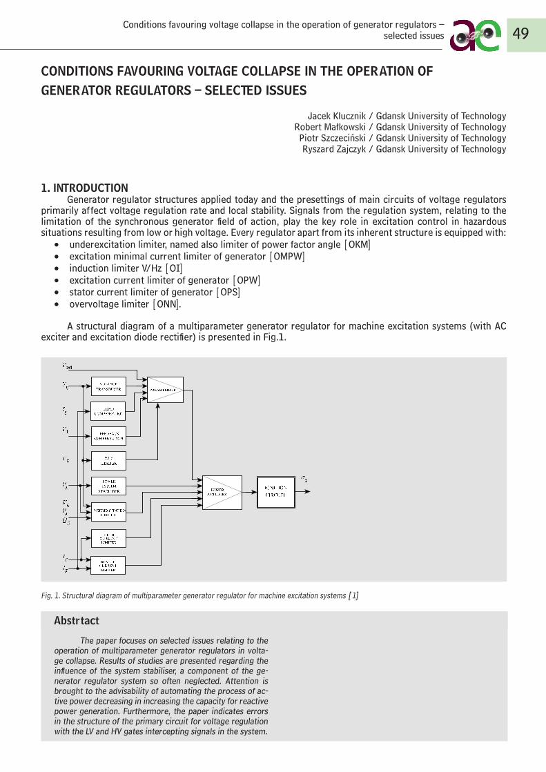
The paper focuses on selected issues relating to the operation of multiparameter generator regulators in volta-ge collapse. Results of studies are presented regarding the influence of the system stabiliser, a component of the ge-nerator regulator system so often neglected. Attention is brought to the advisability of automating the process of ac-tive power decreasing in increasing the capacity for reactive power generation. Furthermore, the paper indicates errors in the structure of the primary circuit for voltage regulation with the LV and HV gates intercepting signals in the system.
Abstrtact
Conditions favouring voltage collapse in the operation of generator regulators – selected issues 49
CONDITIONS FAVOURING VOLTAGE COLLAPSE IN THE OPERATION OF GENERATOR REGULATORS – SELECTED ISSUES
Jacek Klucznik / Gdansk University of TechnologyRobert Małkowski / Gdansk University of TechnologyPiotr Szczeciński / Gdansk University of TechnologyRyszard Zajczyk / Gdansk University of Technology
1. INTRODUCTIONGenerator regulator structures applied today and the presettings of main circuits of voltage regulators
primarily affect voltage regulation rate and local stability. Signals from the regulation system, relating to the limitation of the synchronous generator field of action, play the key role in excitation control in hazardous situations resulting from low or high voltage. Every regulator apart from its inherent structure is equipped with:
• underexcitation limiter, named also limiter of power factor angle [OKM]• excitation minimal current limiter of generator [OMPW]• induction limiter V/Hz [OI]• excitation current limiter of generator [OPW]• stator current limiter of generator [OPS]• overvoltage limiter [ONN].
A structural diagram of a multiparameter generator regulator for machine excitation systems (with AC exciter and excitation diode rectifier) is presented in Fig.1.
Fig. 1. Structural diagram of multiparameter generator regulator for machine excitation systems [1]
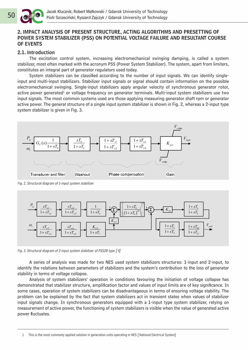
50Jacek Klucznik; Robert Małkowski / Gdansk University of TechnologyPiotr Szczeciński; Ryszard Zajczyk / Gdansk University of Technology
2. IMPACT ANALYSIS OF PRESENT STRUCTURE, ACTING ALGORITHMS AND PRESETTING OF POWER SYSTEM STABILIZER (PSS) ON POTENTIAL VOLTAGE FAILURE AND RESULTANT COURSE OF EVENTS
2.1. IntroductionThe excitation control system, increasing electromechanical swinging damping, is called a system
stabilizer, most often marked with the acronym PSS (Power System Stabilizer). The system, apart from limiters, constitutes an integral part of generator regulators used today.
System stabilizers can be classified according to the number of input signals. We can identify single-input and multi-input stabilizers. Stabilizer input signals or signal should contain information on the possible electromechanical swinging. Single-input stabilizers apply angular velocity of synchronous generator rotor, active power generated1 or voltage frequency on generator terminals. Multi-input system stabilizers use two input signals. The most common systems used are those applying measuring generator shaft rpm or generator active power. The general structure of a single input system stabilizer is shown in Fig. 2, whereas a 2-input type system stabilizer is given in Fig. 3.
Fig. 2. Structural diagram of 1-input system stabilizer
Fig. 3. Structural diagram of 2-input system stabilizer of PSS2B type [4]
A series of analysis was made for two NES used system stabilizers structures: 1-input and 2-input, to identify the relations between parameters of stabilizers and the system’s contribution to the loss of generator stability in terms of voltage collapse.
Analysis of system stabilizers’ operation in conditions favouring the initiation of voltage collapse has demonstrated that stabilizer structure, amplification factor and values of input limits are of key significance. In some cases, operation of system stabilizers can be disadvantageous in terms of ensuring voltage stability. The problem can be explained by the fact that system stabilizers act in transient states when values of stabilizer input signals change. In synchronous generators equipped with a 1-input type system stabilizer, relying on measurement of active power, the functioning of system stabilizers is visible when the value of generated active power fluctuates.
1 This is the most commonly applied solution in generation units operating in NES [National Electrical System]
ee e eeeee
ee e eeeee
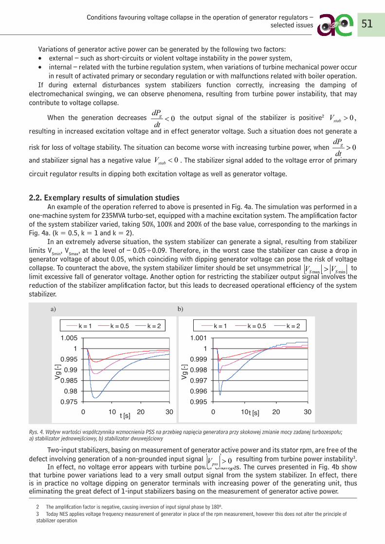
51Conditions favouring voltage collapse in the operation of generator regulators –
selected issues
Variations of generator active power can be generated by the following two factors: • external – such as short-circuits or violent voltage instability in the power system,• internal – related with the turbine regulation system, when variations of turbine mechanical power occur in result of activated primary or secondary regulation or with malfunctions related with boiler operation.If during external disturbances system stabilizers function correctly, increasing the damping of
electromechanical swinging, we can observe phenomena, resulting from turbine power instability, that may contribute to voltage collapse.
When the generation decreases 0gdPdt
> the output signal of the stabilizer is positive2 0stabU < ,
resulting in increased excitation voltage and in effect generator voltage. Such a situation does not generate a
risk for loss of voltage stability. The situation can become worse with increasing turbine power, when 0gdPdt
>
and stabilizer signal has a negative value 0stabU < . The stabilizer signal added to the voltage error of primary
circuit regulator results in dipping both excitation voltage as well as generator voltage.
2.2. Exemplary results of simulation studies An example of the operation referred to above is presented in Fig. 4a. The simulation was performed in a
one-machine system for 235MVA turbo-set, equipped with a machine excitation system. The amplification factor of the system stabilizer varied, taking 50%, 100% and 200% of the base value, corresponding to the markings in Fig. 4a. (k = 0.5, k = 1 and k = 2).
In an extremely adverse situation, the system stabilizer can generate a signal, resulting from stabilizer limits VSmin, VSmax, at the level of – 0.05÷0.09. Therefore, in the worst case the stabilizer can cause a drop in generator voltage of about 0.05, which coinciding with dipping generator voltage can pose the risk of voltage collapse. To counteract the above, the system stabilizer limiter should be set unsymmetrical
max minS SV V> to limit excessive fall of generator voltage. Another option for restricting the stabilizer output signal involves the reduction of the stabilizer amplification factor, but this leads to decreased operational efficiency of the system stabilizer.
Rys. 4. Wpływ wartości współczynnika wzmocnienia PSS na przebieg napięcia generatora przy skokowej zmianie mocy zadanej turbozespołu; a) stabilizator jednowejściowy, b) stabilizator dwuwejściowy
Two-input stabilizers, basing on measurement of generator active power and its stator rpm, are free of the defect involving generation of a non-grounded input signal 0pssU >
resulting from turbine power instability3.
In effect, no voltage error appears with turbine power changes. The curves presented in Fig. 4b show that turbine power variations lead to a very small output signal from the system stabilizer. In effect, there is in practice no voltage dipping on generator terminals with increasing power of the generating unit, thus eliminating the great defect of 1-input stabilizers basing on the measurement of generator active power.
2 The amplification factor is negative, causing inversion of input signal phase by 180º.3 Today NES applies voltage frequency measurement of generator in place of the rpm measurement, however this does not alter the principle of stabilizer operation
4
a) b)
Rys. 4. Wpływ wartości współczynnika wzmocnienia PSS na przebieg napięcia generatora przy skokowej zmianie mocy zadanej turbozespołu; a) stabilizator jednowejściowy, b) stabilizator dwuwejściowy
Wady, polegającej na generowaniu niezerowego sygnału wyjściowego 0pssV > przy zmianach mocy turbiny, pozbawione są stabilizatory dwuwejściowe, bazujące na pomiarze mocy czynnej generatora i prędkości obrotowej wirnika generatora3. Dzięki temu nie powodują one powstawania uchybu napięcia przy zmianach mocy turbiny. Przedstawione na rysunku 4b przebiegi wskazują, Ŝe zmiany mocy turbiny powodują powstawanie bardzo niewielkiego sygnału wyjściowego stabilizatora systemowego. Dzięki temu przy zwiększaniu mocy jednostki wytwórczych praktycznie nie dochodzi do obniŜania napięcia na zaciskach generatora, co było główną wadą stabilizatora jednowejściowego bazującego na pomiarze mocy czynnej generatora.
2.3 Wnioski Analizy prowadzą do następujących wniosków:
• Stabilizatory systemowe jednowejściowe, wykorzystujące pomiar mocy czynnej, mogąprowadzić do obniŜania napięcia generatora przy zmianach mocy turbiny. Wartość o jakąobniŜone zostanie napięcie, zaleŜy od nastaw stabilizatorów – współczynnika wzmocnienie i ograniczników sygnału wyjściowego. Na podstawie nastaw wybranych stabilizatorów stosowanych w KSE moŜna przyjąć, Ŝe maksymalne obniŜenie napięcia na skutek działania stabilizatora moŜe sięgać 5%. Taka wartość w skrajnie niekorzystnych warunkach napięciowych moŜe stanowić zagroŜenie dla utraty stabilności. Rozwiązaniem sytuacji moŜe być blokowanie wzrostu mocy bloku w sytuacji obniŜenia napięcia, co jest równieŜ korzystne z punktu widzenia działania ogranicznika prądu stojana. Drugim rozwiązaniem jest stosowanie stabilizatorów dwuwejściowych, gdzie problem z powstawaniem uchybu napięcia przy zmianach mocy turbiny praktycznie nie występuje
• Nie stwierdzono wpływu stabilizatorów dwuwejściowych na moŜliwość powstania awarii napięciowej. W związku z tym postuluje się instalowanie na wszystkich
3 Obecnie w KSE wykorzystuje się równieŜ pomiar częstotliwości napięcia generatora, zamiast pomiaru prędkości obrotowej, nie zmienia to jednak zasady działania stabilizatorów.
0.9750.98
0.9850.99
0.9951
1.005
0 10 20 30
Vg [-
]
t [s]
k = 1 k = 0.5 k = 2
0.9950.9960.9970.9980.999
11.001
0 10 20 30
Vg [-
]
t [s]
k = 1 k = 0.5 k = 2
e
e
e
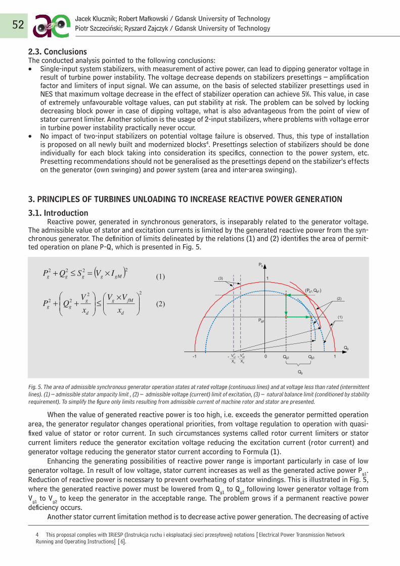
52Jacek Klucznik; Robert Małkowski / Gdansk University of TechnologyPiotr Szczeciński; Ryszard Zajczyk / Gdansk University of Technology
2.3. ConclusionsThe conducted analysis pointed to the following conclusions:• Single-input system stabilizers, with measurement of active power, can lead to dipping generator voltage in
result of turbine power instability. The voltage decrease depends on stabilizers presettings – amplification factor and limiters of input signal. We can assume, on the basis of selected stabilizer presettings used in NES that maximum voltage decrease in the effect of stabilizer operation can achieve 5%. This value, in case of extremely unfavourable voltage values, can put stability at risk. The problem can be solved by locking decreasing block power in case of dipping voltage, what is also advantageous from the point of view of stator current limiter. Another solution is the usage of 2-input stabilizers, where problems with voltage error in turbine power instability practically never occur.
• No impact of two-input stabilizers on potential voltage failure is observed. Thus, this type of installation is proposed on all newly built and modernized blocks4. Presettings selection of stabilizers should be done individually for each block taking into consideration its specifics, connection to the power system, etc. Presetting recommendations should not be generalised as the presettings depend on the stabilizer’s effects on the generator (own swinging) and power system (area and inter-area swinging).
3. PRINCIPLES OF TURBINES UNLOADING TO INCREASE REACTIVE POWER GENERATION
3.1. IntroductionReactive power, generated in synchronous generators, is inseparably related to the generator voltage.
The admissible value of stator and excitation currents is limited by the generated reactive power from the syn-chronous generator. The definition of limits delineated by the relations (1) and (2) identifies the area of permit-ted operation on plane P-Q, which is presented in Fig. 5.
Fig. 5. The area of admissible synchronous generator operation states at rated voltage (continuous lines) and at voltage less than rated (intermittent lines). (1) – admissible stator ampacity limit , (2) – admissible voltage (current) limit of excitation, (3) – natural balance limit (conditioned by stability requirement). To simplify the figure only limits resulting from admissible current of machine rotor and stator are presented.
When the value of generated reactive power is too high, i.e. exceeds the generator permitted operation area, the generator regulator changes operational priorities, from voltage regulation to operation with quasi-fixed value of stator or rotor current. In such circumstances systems called rotor current limiters or stator current limiters reduce the generator excitation voltage reducing the excitation current (rotor current) and generator voltage reducing the generator stator current according to Formula (1).
Enhancing the generating possibilities of reactive power range is important particularly in case of low generator voltage. In result of low voltage, stator current increases as well as the generated active power Pg1. Reduction of reactive power is necessary to prevent overheating of stator windings. This is illustrated in Fig. 5, where the generated reactive power must be lowered from Qg1 to Qg2 following lower generator voltage from Vg1 to Vg2 to keep the generator in the acceptable range. The problem grows if a permanent reactive power deficiency occurs.
Another stator current limitation method is to decrease active power generation. The decreasing of active
4 This proposal complies with IRiESP (Instrukcja ruchu i eksploatacji sieci przesyłowej) notations [Electrical Power Transmission Network Running and Operating Instructions] [6].
5
nowopowstających i modernizowanych blokach tego typu układów4. Dobór nastaw takich stabilizatorów musi odbywać się indywidualnie dla każdego z bloków z uwzględnieniem ich specyfiki, sposobu powiązania z systemem elektroenergetycznym itp. Nie można w sposób ogólny podać zalecanych nastaw, zależą one od efektów, które ma powodować stabilizator w odniesieniu do danego generatora (kołysania własne) i systemu elektroenergetycznego (kołysania obszarowe i międzyobszarowe).
3. Zasady odciążania turbin w celu zwiększenia generacji mocy biernej
3.1 Wstęp
Wartość mocy biernej generowanej przez generator synchroniczny, jest nierozerwalnie związana z wartością napięcia generatora. Ograniczeniem generowanej przez generator synchroniczny mocy biernej jest wartość dopuszczalna prądu stojana i prądu wzbudzenia. Definicja ograniczeń opisanych zależnościami (1) i (2) pozwala na wyznaczenie obszaru dopuszczalnej pracy na płaszczyźnie P-Q, co pokazano na rys. 5.
( )2222gMgggg IUSQP ×=≤+ (1)
2222
⎟⎟⎠
⎞⎜⎜⎝
⎛ ×≤⎟
⎟⎠
⎞⎜⎜⎝
⎛++
d
fMg
d
ggg x
UUx
UQP (2)
Rys. 5. Obszar dopuszczalnych stanów pracy generatora synchronicznego przy napięciu znamionowym (linie ciągłe) i przy napięciu mniejszym do znamionowego (linie przerywane). (1) – granica wynikająca z dopuszczalnej obciążalności prądowej stojana, (2) – granica wynikająca z dopuszczalnego napięcia (prądu) wzbudzenia, (3) – granica równowagi naturalnej (wynikająca z warunku zachowania stabilności). Dla uproszczenia na rysunku
4 Postulat ten jest zgodny z zapisami w IRiESP [6]
5
nowopowstających i modernizowanych blokach tego typu układów4. Dobór nastaw takich stabilizatorów musi odbywać się indywidualnie dla kaŜdego z bloków z uwzględnieniem ich specyfiki, sposobu powiązania z systemem elektroenergetycznym itp. Nie moŜna w sposób ogólny podać zalecanych nastaw, zaleŜą one od efektów, które ma powodowaćstabilizator w odniesieniu do danego generatora (kołysania własne) i systemu elektroenergetycznego (kołysania obszarowe i międzyobszarowe).
3. Zasady odciąŜania turbin w celu zwiększenia generacji mocy biernej 3.1 Wstęp
Wartość mocy biernej generowanej przez generator synchroniczny, jest nierozerwalnie związana z wartością napięcia generatora. Ograniczeniem generowanej przez generator synchroniczny mocy biernej jest wartość dopuszczalna prądu stojana i prądu wzbudzenia. Definicja ograniczeń opisanych zaleŜnościami (1) i (2) pozwala na wyznaczenie obszaru dopuszczalnej pracy na płaszczyźnie P-Q, co pokazano na rys. 5.
( )2222gMgggg IVSQP ×=≤+ (1)
2222
×≤
++
d
fMg
d
ggg x
VVxV
QP (2)
Rys. 5. Obszar dopuszczalnych stanów pracy generatora synchronicznego przy napięciu znamionowym (linie ciągłe) i przy napięciu mniejszym do znamionowego (linie przerywane). (1) – granica wynikająca z dopuszczalnej obciąŜalności prądowej stojana, (2) – granica wynikająca z dopuszczalnego napięcia (prądu) wzbudzenia, (3) – granica równowagi naturalnej (wynikająca z warunku zachowania stabilności). Dla uproszczenia na rysunku
4 Postulat ten jest zgodny z zapisami w IRiESP [6]
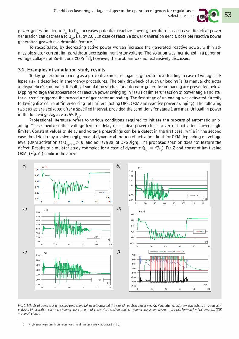
53Conditions favouring voltage collapse in the operation of generator regulators –
selected issues
power generation from Pg1 to Pg2 increases potential reactive power generation in each case. Reactive power generation can decrease to Qg3, i.e. by ∆Qg. In case of reactive power generation deficit, possible reactive power generation growth is a desirable feature.
To recapitulate, by decreasing active power we can increase the generated reactive power, within ad-missible stator current limits, without decreasing generator voltage. The solution was mentioned in a paper on voltage collapse of 26-th June 2006 [2], however, the problem was not extensively discussed.
3.2. Examples of simulation study results Today, generator unloading as a preventive measure against generator overloading in case of voltage col-
lapse risk is described in emergency procedures. The only drawback of such unloading is its manual character at dispatcher’s command. Results of simulation studies for automatic generator unloading are presented below. Dipping voltage and appearance of reactive power swinging in result of limiters reaction of power angle and sta-tor current5 triggered the procedure of generator unloading. The first stage of unloading was activated directly following disclosure of “inter-forcing” of limiters (acting OPS, OKM and reactive power swinging). The following two stages are activated after a specified interval, provided the conditions for stage 1 are met. Unloading power in the following stages was 5% Pgn.
Professional literature refers to various conditions required to initiate the process of automatic unlo-ading. These involve either voltage level or delay or reactive power close to zero at activated power angle limiter. Constant values of delay and voltage presettings can be a defect in the first case, while in the second case the defect may involve negligence of dynamic alteration of activation limit for OKM depending on voltage level (OKM activation at QogrOKM > 0, and no reversal of OPS sign). The proposed solution does not feature the defect. Results of simulator study examples for a case of dynamic Qogr = f(Vg), Fig.7, and constant limit value OKM, (Fig. 6.) confirm the above.
Fig. 6. Effects of generator unloading operation, taking into account the sign of reactive power in OPS. Regulator structure – correction: a) generator voltage, b) excitation current, c) generator current, d) generator reactive power, e) generator active power, f) signals form individual limiters. OGR – overall signal.
5 Problems resulting from inter-forcing of limiters are elaborated in [5].
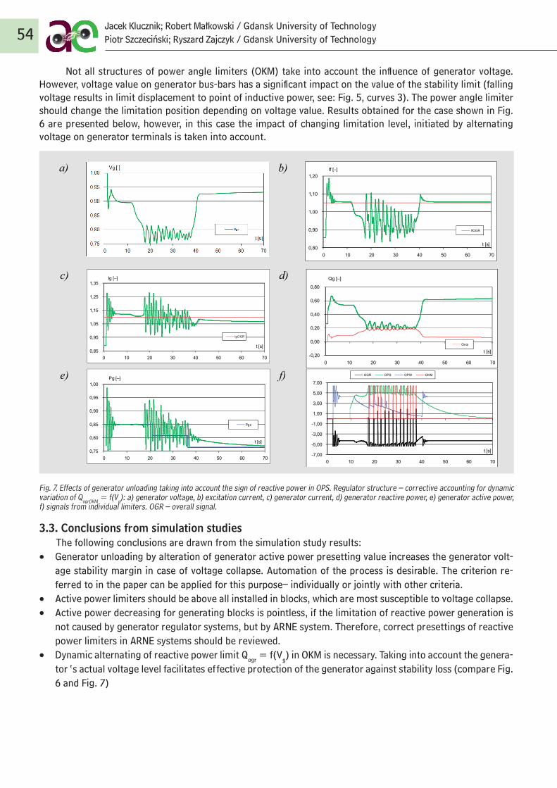
54Jacek Klucznik; Robert Małkowski / Gdansk University of TechnologyPiotr Szczeciński; Ryszard Zajczyk / Gdansk University of Technology
Not all structures of power angle limiters (OKM) take into account the influence of generator voltage. However, voltage value on generator bus-bars has a significant impact on the value of the stability limit (falling voltage results in limit displacement to point of inductive power, see: Fig. 5, curves 3). The power angle limiter should change the limitation position depending on voltage value. Results obtained for the case shown in Fig. 6 are presented below, however, in this case the impact of changing limitation level, initiated by alternating voltage on generator terminals is taken into account.
Fig. 7. Effects of generator unloading taking into account the sign of reactive power in OPS. Regulator structure – corrective accounting for dynamic variation of QogrOKM = f(Vg): a) generator voltage, b) excitation current, c) generator current, d) generator reactive power, e) generator active power, f) signals from individual limiters. OGR – overall signal.
3.3. Conclusions from simulation studies The following conclusions are drawn from the simulation study results:• Generator unloading by alteration of generator active power presetting value increases the generator volt-
age stability margin in case of voltage collapse. Automation of the process is desirable. The criterion re-ferred to in the paper can be applied for this purpose– individually or jointly with other criteria.
• Active power limiters should be above all installed in blocks, which are most susceptible to voltage collapse.• Active power decreasing for generating blocks is pointless, if the limitation of reactive power generation is
not caused by generator regulator systems, but by ARNE system. Therefore, correct presettings of reactive power limiters in ARNE systems should be reviewed.
• Dynamic alternating of reactive power limit Qogr = f(Vg) in OKM is necessary. Taking into account the genera-tor ‘s actual voltage level facilitates effective protection of the generator against stability loss (compare Fig. 6 and Fig. 7)
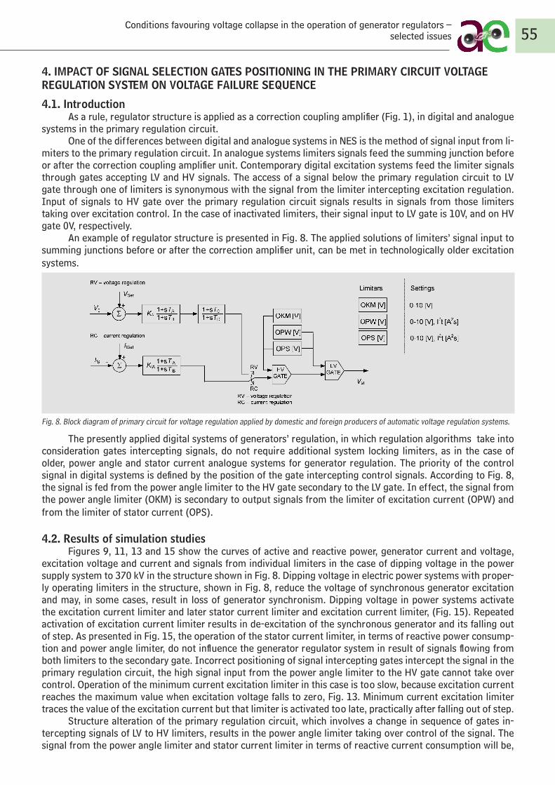
55Conditions favouring voltage collapse in the operation of generator regulators –
selected issues
4. IMPACT OF SIGNAL SELECTION GATES POSITIONING IN THE PRIMARY CIRCUIT VOLTAGE REGULATION SYSTEM ON VOLTAGE FAILURE SEQUENCE
4.1. IntroductionAs a rule, regulator structure is applied as a correction coupling amplifier (Fig. 1), in digital and analogue
systems in the primary regulation circuit.One of the differences between digital and analogue systems in NES is the method of signal input from li-
miters to the primary regulation circuit. In analogue systems limiters signals feed the summing junction before or after the correction coupling amplifier unit. Contemporary digital excitation systems feed the limiter signals through gates accepting LV and HV signals. The access of a signal below the primary regulation circuit to LV gate through one of limiters is synonymous with the signal from the limiter intercepting excitation regulation. Input of signals to HV gate over the primary regulation circuit signals results in signals from those limiters taking over excitation control. In the case of inactivated limiters, their signal input to LV gate is 10V, and on HV gate 0V, respectively.
An example of regulator structure is presented in Fig. 8. The applied solutions of limiters’ signal input to summing junctions before or after the correction amplifier unit, can be met in technologically older excitation systems.
Fig. 8. Block diagram of primary circuit for voltage regulation applied by domestic and foreign producers of automatic voltage regulation systems.
The presently applied digital systems of generators’ regulation, in which regulation algorithms take into consideration gates intercepting signals, do not require additional system locking limiters, as in the case of older, power angle and stator current analogue systems for generator regulation. The priority of the control signal in digital systems is defined by the position of the gate intercepting control signals. According to Fig. 8, the signal is fed from the power angle limiter to the HV gate secondary to the LV gate. In effect, the signal from the power angle limiter (OKM) is secondary to output signals from the limiter of excitation current (OPW) and from the limiter of stator current (OPS).
4.2. Results of simulation studiesFigures 9, 11, 13 and 15 show the curves of active and reactive power, generator current and voltage,
excitation voltage and current and signals from individual limiters in the case of dipping voltage in the power supply system to 370 kV in the structure shown in Fig. 8. Dipping voltage in electric power systems with proper-ly operating limiters in the structure, shown in Fig. 8, reduce the voltage of synchronous generator excitation and may, in some cases, result in loss of generator synchronism. Dipping voltage in power systems activate the excitation current limiter and later stator current limiter and excitation current limiter, (Fig. 15). Repeated activation of excitation current limiter results in de-excitation of the synchronous generator and its falling out of step. As presented in Fig. 15, the operation of the stator current limiter, in terms of reactive power consump-tion and power angle limiter, do not influence the generator regulator system in result of signals flowing from both limiters to the secondary gate. Incorrect positioning of signal intercepting gates intercept the signal in the primary regulation circuit, the high signal input from the power angle limiter to the HV gate cannot take over control. Operation of the minimum current excitation limiter in this case is too slow, because excitation current reaches the maximum value when excitation voltage falls to zero, Fig. 13. Minimum current excitation limiter traces the value of the excitation current but that limiter is activated too late, practically after falling out of step.
Structure alteration of the primary regulation circuit, which involves a change in sequence of gates in-tercepting signals of LV to HV limiters, results in the power angle limiter taking over control of the signal. The signal from the power angle limiter and stator current limiter in terms of reactive current consumption will be,
9
4 Wpływ lokalizacji bramek wybierających sygnał w głównym torze układu regulacji napięcia na przebieg awarii napięciowej
4.1 Wstęp W układach analogowych i cyfrowych w głównym torze regulacji stosuje się z reguły
strukturę regulatora, jako wzmacniacza ze sprzężeniem korekcyjnym, rys. 1. Jedną z różnic w spotykanych w KSE układach analogowych i cyfrowych jest sposób
wprowadzania sygnałów z ograniczników do toru głównego regulacji. W układach analogowych sygnały ograniczników wprowadzane są do węzłów sumacyjnych przed lub za wzmacniaczem z członem korekcyjnym. W stosowanych obecnie cyfrowych układach wzbudzenia stosuje się wprowadzenie sygnałów ograniczników poprzez bramki przejmujące sygnały LV i HV. Wprowadzenie przez jeden z ograniczników do bramki LV wartości mniejszej od sygnału z głównego toru regulacji jest jednoznaczne z przejęciem regulacji wzbudzenia przez sygnał z ogranicznika. Wprowadzenie do bramki HV sygnałów większych od sygnału z toru głównego regulacji, powoduje przejęcie regulacji wzbudzenia przez sygnały z tych ograniczników. Przy niepobudzonych ogranicznikach sygnał z ograniczników wchodzący na bramki LV wynosi 10V, a na bramkę HV odpowiednio 0V.
Przykładową strukturę stosowanych regulatorów przedstawiono na rys. 8. Stosowane rozwiązania z wprowadzaniem sygnałów z ograniczników do węzłów sumacyjnych przed lub za wzmacniaczem z członem korekcyjnym, można spotkać w starszych technologicznie układach wzbudzenia.
Rys. 8. Schemat blokowy toru głównego regulacji napięcia stosowany u krajowych i zagranicznych producentów układów automatycznej regulacji napięcia.
Obecnie stosowane cyfrowe układy regulacji generatorów, których algorytmy regulacji uwzględniają stosowanie bramek przejmujących sygnał, nie wymagają dodatkowych układów blokujących ograniczniki, jak to jest w ogranicznikach kąta mocy i ogranicznikach prądu stojana w starszych, analogowych układach regulacji generatorów. Nadrzędność sygnału sterowania w układach cyfrowych jest definiowana kolejnością rozmieszczenia bramek przejmujących sygnały sterujące. Zgodnie z rys. 8 sygnał z ogranicznika kąta mocy jest wprowadzany do bramki HV, podrzędnej względem bramki LV. Powoduje to, że sygnał z ogranicznika kąta mocy (OKM) jest podrzędny względem sygnałów z ogranicznika prądu wzbudzenia (OPW) i z ogranicznika prądu stojana (OPS).
4.2 Wyniki badań symulacyjnych Na rys. 9, 11, 13 i 15 przedstawiono przebiegi mocy czynnej i mocy biernej, prądu i
napięcia generatora, napięcia i prądu wzbudzenia oraz sygnały z poszczególnych
e e e eeee
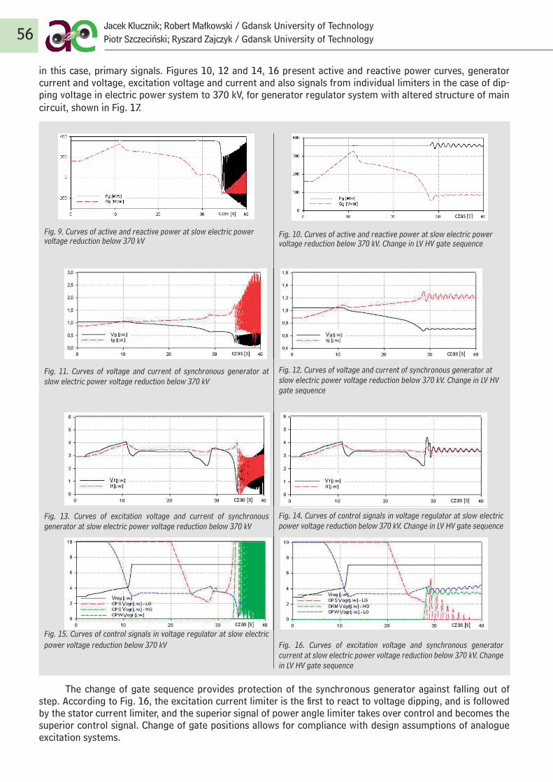
56Jacek Klucznik; Robert Małkowski / Gdansk University of TechnologyPiotr Szczeciński; Ryszard Zajczyk / Gdansk University of Technology
in this case, primary signals. Figures 10, 12 and 14, 16 present active and reactive power curves, generator current and voltage, excitation voltage and current and also signals from individual limiters in the case of dip-ping voltage in electric power system to 370 kV, for generator regulator system with altered structure of main circuit, shown in Fig. 17.
Fig. 9. Curves of active and reactive power at slow electric power voltage reduction below 370 kV
Fig. 10. Curves of active and reactive power at slow electric power voltage reduction below 370 kV. Change in LV HV gate sequence
Fig. 11. Curves of voltage and current of synchronous generator at slow electric power voltage reduction below 370 kV
Fig. 12. Curves of voltage and current of synchronous generator at slow electric power voltage reduction below 370 kV. Change in LV HV gate sequence
Fig. 13. Curves of excitation voltage and current of synchronous generator at slow electric power voltage reduction below 370 kV
Fig. 14. Curves of control signals in voltage regulator at slow electric power voltage reduction below 370 kV. Change in LV HV gate sequence
Fig. 15. Curves of control signals in voltage regulator at slow electric power voltage reduction below 370 kV Fig. 16. Curves of excitation voltage and synchronous generator
current at slow electric power voltage reduction below 370 kV. Change in LV HV gate sequence
The change of gate sequence provides protection of the synchronous generator against falling out of step. According to Fig. 16, the excitation current limiter is the first to react to voltage dipping, and is followed by the stator current limiter, and the superior signal of power angle limiter takes over control and becomes the superior control signal. Change of gate positions allows for compliance with design assumptions of analogue excitation systems.
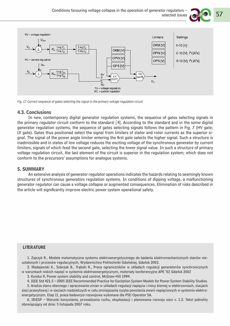
57Conditions favouring voltage collapse in the operation of generator regulators –
selected issues
Σ+
- 1+sTA1+sTB
KA1+sTC1+sTD
HVGATELV
GATE
OKM [V]
UNast
Ug
OPW [V]
OPS [V]
OKM [V]
OPW [V]
OPS [V]
Ust
RA
RRRA – regulacja automatycznaRR – regulacja ręczna
Σ+
- 1+sTIA1+sTIB
KIA
IfNast
Ifg
RA – regulacja automatyczna
RR – regulacja ręczna
0-10 [V]
0-10 [V], I2t [A2s]
0-10 [V], I2t [A2s]
Ograniczniki: Nastawy:
Fig. 17. Correct sequence of gates selecting the signal in the primary voltage regulation circuit
4.3. ConclusionsIn new, contemporary digital generator regulation systems, the sequence of gates selecting signals in
the primary regulator circuit conform to the standard [4]. According to the standard and in the some digital generator regulation systems, the sequence of gates selecting signals follows the pattern in Fig. 7 (HV gate; LV gate). Gates thus positioned select the signal from limiters of stator and rotor currents as the superior si-gnal. The signal of the power angle limiter entering the first gate selects the higher signal. Such a structure is inadmissible and in states of low voltage reduces the exciting voltage of the synchronous generator by current limiters, signals of which feed the second gate, selecting the lower signal value. In such a structure of primary voltage regulation circuit, the last element of the circuit is superior in the regulation system; which does not conform to the precursors’ assumptions for analogue systems.
5. SUMMARYAn extensive analysis of generator regulator operations indicates the hazards relating to seemingly known
structures of synchronous generators regulation systems. In conditions of dipping voltage, a malfunctioning generator regulator can cause a voltage collapse or augmented consequences. Elimination of risks described in the article will significantly improve electric power system operational safety.
LITERATURE
1. Zajczyk R., Modele matematyczne systemu elektroenergetycznego do badania elektromechanicznych stanów nie-ustalonych i procesów regulacyjnych, Wydawnictwo Politechniki Gdańskiej, Gdańsk 2003.
2. Madajewski K., Sobczak B., Trębski R., Praca ograniczników w układach regulacji generatorów synchronicznych w warunkach niskich napięć w systemie elektroenergetycznym, materiały konferencyjne APE ’07, Gdańsk 2007.
3. Kundur P., Power system stability and control, McGraw-Hill 1994.4. IEEE Std 421.5 – 2005 IEEE Recommended Practice for Excitation System Models for Power System Stability Studies.5. Analiza stanu obecnego i opracowanie zmian w układach regulacji napięcia i mocy biernej w elektrowniach, stacjach
sieci przesyłowej i w sieciach rozdzielczych w celu zmniejszenia ryzyka powstania awarii napięciowych w systemie elektro-energetycznym. Etap II, praca badawczo-rozwojowa wykonana dla PSE-Operator SA.
6. IRiESP – Warunki korzystania, prowadzenia ruchu, eksploatacji i planowania rozwoju sieci v. 1.2. Tekst jednolity obowiązujący od dnia: 5 listopada 2007 roku.

Authors / Biographies
Jerzy KulczyckiKraków / Poland Graduate of Silesian University of Technology in Gliwice (1956). He was awarded PhD in AGH University of Science and Technology in Kraków (1967), then, in 1976 - second level doctorate (habilitation) and became a professor in 1991. During the period of 1956–72 he worked mainly at installment and project design of electrical power systems. Since 1972 – an academic teacher in AGH University of Science and Technology. His profes-sional interests include electrical power engineer-ing, in particular, methods of designing optimum system structures, enhanced efficiency of using of electrical power systems.
Waldemar L. SzpyraKraków / Poland
He obtained the diploma of engineer electri-cian in the Faculty of Electrical Engineering of AGH University of Science and Technology in Kraków in 1975, and PhD – in the Faculty of Electrical Engineering, Automatics, IT and Electronics of AGH University of Science and Technology in Kraków in 1998. Now - an assist-ant professor in the Department of Electrical and Power Engineering of his University. He deal with modelling, state estimation and optimal control of power distribution networks using an artificial intelligence methods and electrical power management.
Michał Rudziński Kraków / Poland
Graduate of the Faculty of Faculty of Electrical Engi-neering, Automatics and Electronics of AGH University of Science and Technology in Kraków. He was awarded Master’s – engineer’s degree in electrical automation and metrology in 1979. During the period of 1979–1983 he worked in Kielce in research and development center of industrial fittings (Ośrodek Badawczo-Roz-wojowy Armatury Przemysłowej). During the period of 1983–1995 he was employed in T. Sendzimir steel-works in Kraków as a specialist in Power Engineering Division. Since 1995 he as been working in electrical power distribution company ENION S.A. in Kraków as the Head of Transmission Services Management Office. Member of numerous working groups appointed by Polskie Towarzystwo Przesyłu i Rozdziału Energii Ele-ktrycznej (Polish Society of Electrical Energy Transfer and Distribution).
58Jerzy Kulczycki; Waldemar L. Szpyra/ AGH University of Science and Technology in CracowMichał Rudziński / ENION S.A.
Abstract
POWER LOSSES AS NECESSARY OWN NEEDS OF NETWORK
Jerzy Kulczycki / AGH University of Science and Technology in Cracow Michał Rudziński / ENION S.A.
Waldemar Szpyra / AGH University of Science and Technology in Cracow
1. CAUSES OF LOSSES; ACTUAL, JUSTIFIED AND OPTIMAL LOSSES Output energy is smaller than input energy in each element of energy network.Network energy losses are the difference between the energy introduced into the network and the power
received from the network. Network losses are most often classified by their sources of origin. Technical losses and commercial losses are distinguished.
Technical losses of power are due to physical phenomena accompanying power flow in network or voltage in network. Based on these phenomena, the following classification is adopted:
• current losses (load, lengthwise losses) dependent on load (Joule heat)• voltage losses (idle, crosswise losses) dependent on voltage (losses in dielectrics, losses of corona dis-
charge, losses in transformer cores).Technical power losses are unavoidable in a network consisting of the elements in which those phenomena
occur. Since each element of a network has resistance – flow of current produces heat, which is a loss of a part of the power transmitted. Live insulation also produces losses. Losses in resistance and in insulation of properly selected and used element of a network result from “the physics of the phenomena” taking place during power transmission. They do not occur due to wastefulness or mismanagement. It seems that own needs of network or, to be more precise, power own needs of network would be a more appropriate term to describe such losses. However, the term technical losses will be used in further parts of the text; as it is shorter, generally understood and generally used.
Commercial losses are due to the fact that both input energy, and output energy are measured with certain errors. They are thus effects of energy trading issues. They are classified in the following way:
• losses due to errors of measurement systems, mainly from high start up level of meters and accuracy class of the meters used - it can happen that losses due to errors of measurement systems are less than zero
• losses resulting from registration system of energy sold, e.g. resulting from the system adopted for set-tlement, based on forecasts of energy consumption by small consumers. Losses in the case of different frequency of reading of various groups of meters and delays in meter readings constitute other examples of regulation losses. Regulation losses have positive and negative values, and in longer time periods their value is close to zero
• unmeasured energy taken from network (illegal energy consumption).
Power Losses as Necessary Own Needs of Network 59
Classification of network losses (balance difference) by sources of their origin was presented. It was demonstra-ted that balance difference is not sufficient to determine the technical losses in the network. Due to measurement errors and errors resulting from energy sold registration systems, balance difference often shows, in relation to actual losses, alternately inflated, underestimated or even negative valu-es. Three methods of calculating actual losses based on reporting were presented. Impact of local energy sources, energy transits, distribution network operator decisions and contractual obligations with some consumers on losses fac-tor were pointed out to.
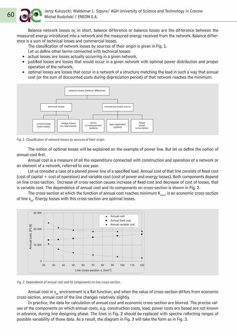
Balance network losses or, in short, balance difference or balance losses are the difference between the measured energy introduced into a network and the measured energy received from the network. Balance differ-ence is a sum of technical losses and commercial losses.
The classification of network losses by sources of their origin is given in Fig. 1.Let us define other terms connected with technical losses:
• actual losses are losses actually occurring in a given network, • justified losses are losses that would occur in a given network with optimal power distribution and proper
operation of the network,• optimal losses are losses that occur in a network of a structure matching the load in such a way that annual
cost (or the sum of discounted costs during depreciation period) of that network reaches the minimum.
Fig. 1. Classification of network losses by sources of their origin
The notion of optimal losses will be explained on the example of power line. But let us define the notion of annual cost first.
Annual cost is a measure of all the expenditure connected with construction and operation of a network or an element of a network, referred to one year.
Let us consider a case of a planed power line of a specified load. Annual cost of that line consists of fixed cost (cost of capital + cost of operation) and variable cost (cost of power and energy losses). Both components depend on line cross-section. Increase of cross-section causes increase of fixed cost and decrease of cost of losses, that is variable cost. The dependence of annual cost and its components on cross-section is shown in Fig. 2.
The cross-section at which the function of annual cost reaches minimum Krmin, is an economic cross-section of line sek. Energy losses with this cross-section are optimal losses.
Fig. 2. Dependence of annual cost and its components on line cross-section.
Annual cost in sek environment is a flat function, and when the value of cross-section differs from economic cross-section, annual cost of the line changes relatively slightly.
In practice, the data for calculation of annual cost and economic cross-section are blurred. The precise val-ues of the components on which annual costs, e.g. construction costs, load, power costs are based are not known in advance, during line designing phase. The lines in Fig. 2 should be replaced with spectra reflecting ranges of possible variability of those data. As a result, the diagram in Fig. 2 will take the form as in Fig. 3.
60Jerzy Kulczycki; Waldemar L. Szpyra/ AGH University of Science and Technology in CracowMichał Rudziński / ENION S.A.
2
losses. Regulation losses have positive and negative values, and in longer time periods their value is close to zero unmeasured power energy taken from network (illegal power energy consumption).
Balance network losses or, in short, balance difference or balance losses are the difference between the measured power energy introduced into a network and the measured power energy received from the network. Balance difference is a sum of technical losses and commercial losses.
The classification of network losses by sources of their origin is given in Fig. 1. Let us define other terms connected with technical losses:
actual losses are losses actually occurring in a given network, justified losses are losses that would occur in a given network with optimal power
distribution and proper operation of the network, optimal losses are losses that occur in a network of a structure matching the load in
such a way that annual cost (or the sum of discounted costs during depreciation period) of that network reaches the minimum.
Fig. 1. Classification of network losses by sources of their origin
The notion of optimal losses will be explained on the example of power line. But
let us define the notion of annual cost first. Annual cost is a measure of all the expenditure connected with construction and
operation of a network or an element of a network, referred to one year. Let us consider a case of a planed power line of a specified load. Annual cost of
that line consists of fixed cost (cost of capital + cost of operation) and variable cost (cost of power and energy losses). Both components depend on line cross-section. Increase of cross-section causes increase of fixed cost and decrease of cost of losses, that is floating variable cost. The dependence of annual cost and its components on cross-section is shown in Fig. 2.
The cross-section at which the function of annual cost reaches minimum Krmin, is an economic cross-section of line sek. Power Energy losses with this cross-section are optimal losses.
balance losses (balance difference)
technical losses
current losses (load losses)
voltage losses (no load losses)
commercial losses due to:
errors of measurement
systems sale registration
systems
illegal power
consumption
3
Fig. 2. Dependence of annual cost and its components on line cross-section.
Annual cost in sek environment is a flat function, and when the value of cross-
section differs from economic cross-section, annual cost of the line changes relatively slightly.
In practice, the data for calculation of annual cost and economic cross-section are blurred. The precise values of the components on which annual costs, e.g. construction costs, load, power costs are based are not known in advance, during line designing phase. The lines in Fig. 2 should be replaced with spectra reflecting ranges of possible variability of those data. As a result, the diagram in Fig. 2 will take the form as in Fig. 3.
Fig. 3. Dependence of annual cost and its components on line cross-section in the case of “blurred” cost data – broken line shows borders of variability of costs with the assumption that investment expenditure and power losses bear an error of ±5%.
0
10 000
20 000
30 000
20 30 40 50 60 70 80 90 100 110 120 Line cross-section s, [mm2]
Ann
ual c
ost,
[PLN
]
Annual cost Annual fixed cost Annual variable cost
0
10 000
20 000
30 000
20 30 40 50 60 70 80 90 100 110 120 Line cross-section s, [mm2]
Ann
ual c
ost,
[PLN
]
Annual cost Annual fixed cost Annual variable cost
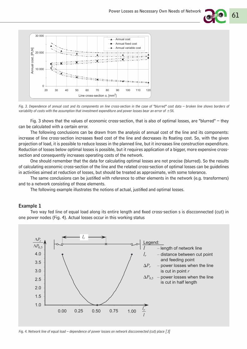
Fig. 3. Dependence of annual cost and its components on line cross-section in the case of “blurred” cost data – broken line shows borders of variability of costs with the assumption that investment expenditure and power losses bear an error of ±5%.
Fig. 3 shows that the values of economic cross-section, that is also of optimal losses, are “blurred” – they can be calculated with a certain error.
The following conclusions can be drawn from the analysis of annual cost of the line and its components: increase of line cross-section increases fixed cost of the line and decreases its floating cost. So, with the given projection of load, it is possible to reduce losses in the planned line, but it increases line construction expenditure. Reduction of losses below optimal losses is possible, but it requires application of a bigger, more expensive cross-section and consequently increases operating costs of the network.
One should remember that the data for calculating optimal losses are not precise (blurred). So the results of calculating economic cross-section of the line and the related cross-section of optimal losses can be guidelines in activities aimed at reduction of losses, but should be treated as approximate, with some tolerance.
The same conclusions can be justified with reference to other elements in the network (e.g. transformers) and to a network consisting of those elements.
The following example illustrates the notions of actual, justified and optimal losses.
Example 1Two way fed line of equal load along its entire length and fixed cross-section s is discconnected (cut) in
one power nodes (Fig. 4). Actual losses occur in this working status
Fig. 4. Network line of equal load – dependence of power losses on network discconnected (cut) place [3]
61Power Losses as Necessary Own Needs of Network
3
Fig. 2. Dependence of annual cost and its components on line cross-section.
Annual cost in sek environment is a flat function, and when the value of cross-
section differs from economic cross-section, annual cost of the line changes relatively slightly.
In practice, the data for calculation of annual cost and economic cross-section are blurred. The precise values of the components on which annual costs, e.g. construction costs, load, power costs are based are not known in advance, during line designing phase. The lines in Fig. 2 should be replaced with spectra reflecting ranges of possible variability of those data. As a result, the diagram in Fig. 2 will take the form as in Fig. 3.
Fig. 3. Dependence of annual cost and its components on line cross-section in the case of “blurred” cost data – broken line shows borders of variability of costs with the assumption that investment expenditure and power losses bear an error of ±5%.
0
10 000
20 000
30 000
20 30 40 50 60 70 80 90 100 110 120 Line cross-section s, [mm2]
Ann
ual c
ost,
[PLN
]
Annual cost Annual fixed cost Annual variable cost
0
10 000
20 000
30 000
20 30 40 50 60 70 80 90 100 110 120 Line cross-section s, [mm2]
Ann
ual c
ost,
[PLN
]
Annual cost Annual fixed cost Annual variable cost
4
Fig. 3 shows that the values of economic cross-section, that is also of optimal
losses, are “blurred” – they can be calculated with a certain error. The following conclusions can be drawn from the analysis of annual cost of the
line and its components: increase of line cross-section increases fixed cost of the line and decreases its floating cost. So, with the given projection of load, it is possible to reduce losses in the planned line, but it increases line construction expenditure. Reduction of losses below optimal losses is possible, but it requires application of a bigger, more expensive cross-section and consequently increases operating costs of the network.
One should remember that the data for calculating optimal losses are not precise (blurred). So the results of calculating economic cross-section of the line and the related cross-section of optimal losses can be guidelines in activities aimed at reduction of losses, but should be treated as approximate, with some tolerance.
The same conclusions can be justified with reference to other elements in the network (e.g. transformers) and to a network consisting of those elements.
The following example illustrates the notions of actual, justified and optimal losses.
Example 1 Two way fed line of equal load along its entire length and fixed cross-section s is
disconnected (cut) in one power nodes (Fig. 4). Actual losses occur in this working status.
Fig. 4. Network line of equal load – dependence of power losses on network disconnection (cut) place [3]
In a two way fed line of equal load along its entire length, but cut, actual losses depend on location of cut point. The dependence is shown in Fig. 4. If there were no contraindications for change of cut point (e.g. resulting from the requirement of
1.0
1.5
2.0
2.5
3.0
3.5
4.0
0.00 0.25 0.50 0.75 1.00
Legend: l – length of network line lr – distance between cut point
and feeding point Pr – power losses when the line
is cut in point r P0,5 – power losses when the line
is cut in half length
lr
5,0PPr
llr
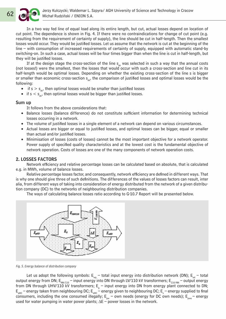
In a two way fed line of equal load along its entire length, but cut, actual losses depend on location of cut point. The dependence is shown in Fig. 4. If there were no contraindications for change of cut point (e.g. resulting from the requirement of certainty of supply), the line should be cut in half-length. Then the smallest losses would occur. They would be justified losses. Let us assume that the network is cut at the beginning of the line – with consumption of increased requirements of certainty of supply, equipped with automatic stand-by switching-on. In such a case, actual losses will be four times bigger than when the line is cut in half-length, but they will be justified losses.
If at the design stage the cross-section of the line sek was selected in such a way that the annual costs (not losses!) were the smallest, then the losses that would occur with such a cross-section and line cut in its half-length would be optimal losses. Depending on whether the existing cross-section of the line s is bigger or smaller than economic cross-section sek, the comparison of justified losses and optimal losses would be the following:
• if s > sek, then optimal losses would be smaller than justified losses• if s < sek, then optimal losses would be bigger than justified losses.
Sum upIt follows from the above considerations that:
• Balance losses (balance difference) do not constitute sufficient information for determining technical losses occurring in a network.
• The volume of justified losses in a single element of a network can depend on various circumstances.• Actual losses are bigger or equal to justified losses, and optimal losses can be bigger, equal or smaller
than actual and/or justified losses.• Minimisation of losses (costs of losses) cannot be the most important objective for a network operator.
Power supply of specified quality characteristics and at the lowest cost is the fundamental objective of network operation. Costs of losses are one of the many components of network operation costs.
2. LOSSES FACTORS Network efficiency and relative percentage losses can be calculated based on absolute, that is calculated
e.g. in MWh, volume of balance losses.Relative percentage losses factor, and consequently, network efficiency are defined in different ways. That
is why one should give three of such definitions. The differences of the values of losses factors can result, inter alia, from different ways of taking into consideration of energy distributed from the network of a given distribu-tion company (DC) to the networks of neighbouring distribution companies.
The ways of calculating balance losses ratio according to G-10.7 Report will be presented below.
Fig. 5. Energy balance of distribution company
Let us adopt the following symbols: Ewp – total input energy into distribution network (DN); Eod – total output energy from DN; ENN/110 – input energy into DN through LV/110 kV transformers; E110/NN – output energy from DN through UHV/110 kV transformers; Eg – input energy into DN from energy plant connected to DN; EpDC – energy taken from neighbouring DC; EoDC – energy given to neighbouring DC; Es – energy supplied to final consumers, including the one consumed illegally; Epw – own needs (energy for DC own needs); Epwe – energy used for water pumping in water power plants; ∆E – power losses in the network.
62Jerzy Kulczycki; Waldemar L. Szpyra/ AGH University of Science and Technology in CracowMichał Rudziński / ENION S.A.
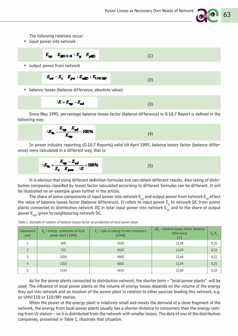
The following relations occur:• input power into network
(1)
• output power from network
(2)
• balance losses (balance difference, absolute value)
(3)
Since May 1995, percentage balance losses factor (balance difference) in G-10.7 Report is defined in the following way:
(4)
In power industry reporting (G.10.7 Reports) valid till April 1995, balance losses factor (balance differ-ence) were calculated in a different way, that is:
(5)
It is obvious that using different definition formulas one can obtain different results. Also rating of distri-bution companies classified by losses factor calculated according to different formulas can be different. It will be illustrated on an example given further in the article.
The share of some components of input power into network Ewp and output power from network Eod affect the value of balance losses factor (balance difference). It refers to input power Eg to network DC from power plants connected to distribution network DC in total input power into network Ewp and to the share of output power EoSD given to neighbouring network DC.
Table 1. Example of relation of balance losses factor on production of local power plant
Subsequent year
Eg – energy production of local power plant [GWh]
Es – sale of energy to end consumers[GWh]
∆E% – balance losses factor (balance difference)
[%]Eg/Es
1 890 4336 13,96 0,21
2 752 4559 14,99 0,16
3 1026 4805 13,68 0,21
4 1014 4682 13,04 0,22
5 1544 4642 12,00 0,33
As for the power plants connected to distribution network, the shorter term – “local power plants” will be used. The influence of local power plants on the volume of energy losses depends on the volume of the energy they put into network and on location of the power plant in relation to other sources feeding this network, e.g. on UHV/110 or 110/MV station.
When the power of the energy plant is relatively small and meets the demand of a close fragment of the network, the energy from local power plants usually has a shorter distance to consumers than the energy com-ing from LV station – so it is distributed from the network with smaller losses. The data of one of the distribution companies, presented in Table 1, illustrate that situation.
63Power Losses as Necessary Own Needs of Network

And when a local power plant also covers the load of distant consumers, e.g. surplus of input power into network at a given voltage is transformed into higher voltage – the work of the local power plant can increase power losses.
If a local power plant puts power into 110 kV network of the power of hundreds MW distributed in a few 110 kV networks, power losses in some distribution networks will decrease, and in some – they will increase; but:
• the biggest growth of losses occurs in a network of that distribution network to which the local power plant is connected
• losses in all distribution networks calculated together can increase or decreaseTables 2 and 3 refer to such a situation.
Table 2. An example of dependencies of balance losses factor in four distribution networks and in a 110 kV network of national power system (KSE) on the work of local power plant (heat and power generating plant) of 500 MW, connected to network DC-1
Variant
Power losses in MW in a 110 kV network of four distribution networks and a network of national power system (KSE), planned winter peak demand - 2015
DC-1 DC-2 DC-3 DC-4 KSE network
Initial 17,8 13,3 11,5 27,9
After launching of heat and power generating plant of the power of 500 MW 31,1 12,5 10,5 22,5
Effect of launching heat and power generating plant +13,3 –0,8 –1,0 –5,4 +6,3
Table 3. An example of dependencies of balance losses factor in five distribution networks and in a KSE 110 kV network on work of two heat and power generating plants of combined power of 330 MW, connected to distribution network DC-2
Variant
Power losses in MW in a 110 kV network of five distribution networks and the network of national power system (KSE), planned winter peak demand - 2015
SD-1 SD-2 SD-3 SD-4 SD-5 KSE network
Initial 17,8 13,3 11,5 27,9 10,8
After launching of heat and power generating plant of the power of 500 MW 16,1 14,9 10,6 26,4 11,9
Effect of launching heat and power generating plant -1,7 +1,6 –0,9 –1,5 +1,1 –1,4
Most of power transit to neighbouring distribution networks is in 110 kV, which is connected with consid-erably smaller percentage losses than power distribution to end users, fed at lower voltage levels. In the case of power transit (giving power do neighbouring distribution networks), percentage losses are smaller and network efficiency - bigger. The following calculation example explains it:
Example 2
Fig. 6. Energy balance of distribution companies – influence of calculation methodology on the volume of balance losses factor (balance difference)
Balance losses factors (balance difference) for distribution companies with energy balance as in Fig. 6 [formula (4)] are as follows:
• distribution company A
64Jerzy Kulczycki; Waldemar L. Szpyra/ AGH University of Science and Technology in CracowMichał Rudziński / ENION S.A.
9
power generating plant Most of power transit to neighbouring distribution networks is in 110 kV, which
is connected with considerably smaller percentage losses than power distribution to end users, fed at lower voltage levels. In the case of power transit (giving power do neighbouring distribution networks), percentage losses are smaller and network efficiency - bigger. The following calculation example explains it:
Example 2
Fig. 6. Power Energy balance of distribution companies – influence of calculation methodology on the volume of balance losses factor (balance difference)
Balance losses factors (balance difference) for distribution companies with power
energy balance as in Fig. 6 [formula (4)] are as follows: distribution company A
%09.9%100110
100110%100%wp
odwp
EEE
E
distribution company B
%20.7%100150
2.139150%E
And the factors calculated by the use of the method valid till to April 1995 [formula (5)] are as follows: distribution company A
%09.9%10010100
100110%100% EEEEE
Epwes
odwp
DC A area
ENN/110 110
Es 100
ΔE 10
DC B area
ENN/110 150
Es 100
ΔE 10.8
EoSD 39.2
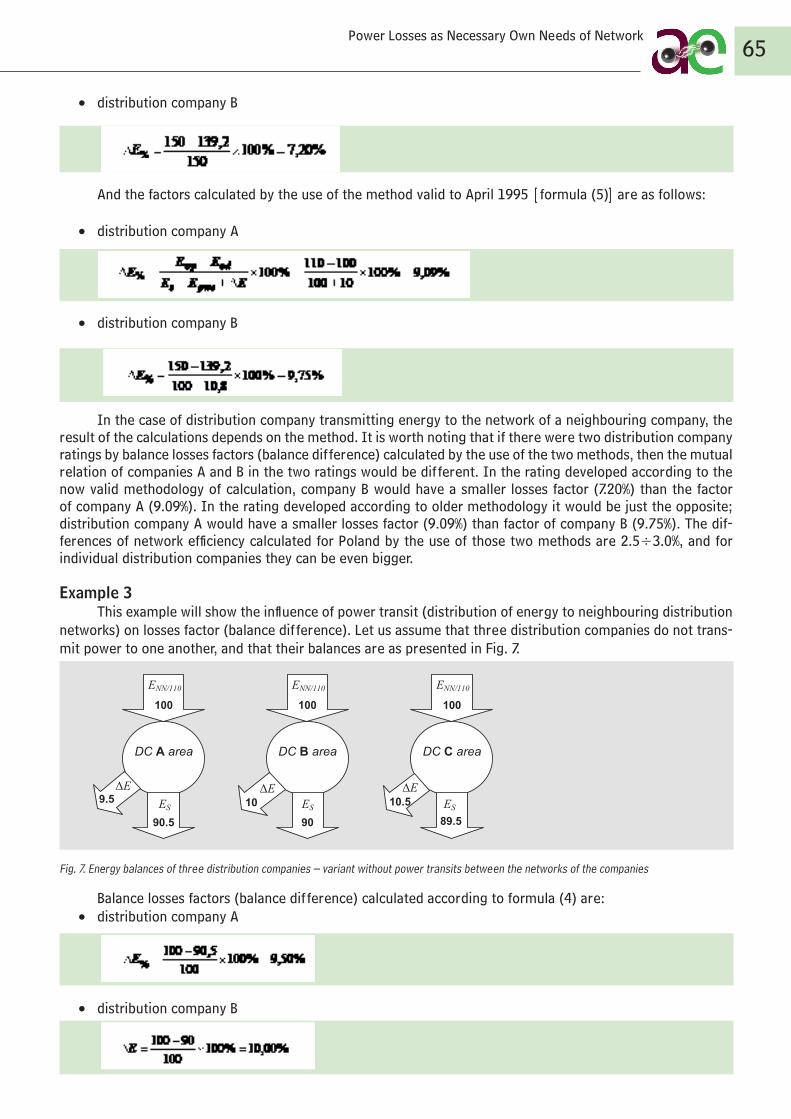
• distribution company B
And the factors calculated by the use of the method valid to April 1995 [formula (5)] are as follows:
• distribution company A
• distribution company B
In the case of distribution company transmitting energy to the network of a neighbouring company, the result of the calculations depends on the method. It is worth noting that if there were two distribution company ratings by balance losses factors (balance difference) calculated by the use of the two methods, then the mutual relation of companies A and B in the two ratings would be different. In the rating developed according to the now valid methodology of calculation, company B would have a smaller losses factor (7.20%) than the factor of company A (9.09%). In the rating developed according to older methodology it would be just the opposite; distribution company A would have a smaller losses factor (9.09%) than factor of company B (9.75%). The dif-ferences of network efficiency calculated for Poland by the use of those two methods are 2.5÷3.0%, and for individual distribution companies they can be even bigger.
Example 3This example will show the influence of power transit (distribution of energy to neighbouring distribution
networks) on losses factor (balance difference). Let us assume that three distribution companies do not trans-mit power to one another, and that their balances are as presented in Fig. 7.
Fig. 7. Energy balances of three distribution companies – variant without power transits between the networks of the companies
Balance losses factors (balance difference) calculated according to formula (4) are:• distribution company A
• distribution company B
65Power Losses as Necessary Own Needs of Network
10
distribution company B
%75.9%1008.101002.139150
%E
In the case of distribution company transmitting power energy to the network of a neighbouring company, the result of the calculations depends on the method. It is worth noting that if there were two distribution company ratings by balance losses factors (balance difference) calculated by the use of the two methods, then the mutual relation of companies A and B in the two ratings would be different. In the rating developed according to the now valid methodology of calculation, company B would have a smaller losses factor (7.20%) than the factor of company A (9.09%). In the rating developed according to older methodology it would be just the opposite; distribution company A would have a smaller losses factor (9.09%) than factor of company B (9.75%). The differences of network efficiency calculated for Poland by the use of those two methods are 2.5÷3.0%, and for individual distribution companies they can be even bigger.
Example 3 This example will show the influence of power transit (distribution of power
energy to neighbouring distribution networks) on losses factor (balance difference). Let us assume that three distribution companies do not transmit power to one another, and that their balances are as presented in Fig. 7.
Fig. 7. Power Energy balances of three distribution companies – variant without power transits between the networks of the companies
Balance losses factors (balance difference) calculated according to formula (4) are: distribution company A
DC A area
ENN/110 100
ES 90.5
ΔE 9.5
DC B area
ES 90
ΔE 10
DC C area
89.5
ΔE 10.5
ENN/110 100
ENN/110 100
ES
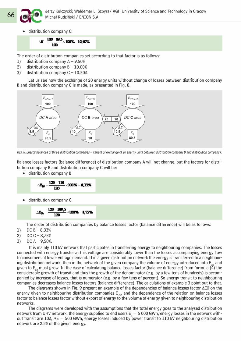
• distribution company C
The order of distribution companies set according to that factor is as follows:1) distribution company A – 9.50%2) distribution company B – 10.00%3) distribution company C – 10.50%
Let us see how the exchange of 20 energy units without change of losses between distribution company B and distribution company C is made, as presented in Fig. 8.
Rys. 8. Energy balances of three distribution companies – variant of exchange of 20 energy units between distribution company B and distribution company C
Balance losses factors (balance difference) of distribution company A will not change, but the factors for distri-bution company B and distribution company C will be:
• distribution company B
• distribution company C
The order of distribution companies by balance losses factor (balance difference) will be as follows:1) DC B – 8,33%2) DC C – 8,75%3) DC A – 9,50%.
It is mainly 110 kV network that participates in transferring energy to neighbouring companies. The losses connected with energy transfer at this voltage are considerably lower than the losses accompanying energy flow to consumers of lower voltage demand. If in a given distribution network the energy is transferred to a neighbour-ing distribution network, then in the network of the given company the volume of energy introduced into Ewp and given to Eod must grow. In the case of calculating balance losses factor (balance difference) from formula (4) the considerable growth of transit and thus the growth of the denominator (e.g. by a few tens of hundreds) is accom-panied by increase of losses, that is numerator (e.g. by a few tens of percent). So energy transit to neighbouring companies decreases balance losses factors (balance difference). The calculations of example 3 point out to that.
The diagrams shown in Fig. 9 present an example of the dependencies of balance losses factor ∆E% on the energy given to neighbouring distribution companies EoSD and the dependence of the relation on balance losses factor to balance losses factor without export of energy to the volume of energy given to neighbouring distribution networks.
The diagrams were developed with the assumptions that the total energy goes to the analysed distribution network from UHV network, the energy supplied to end users Es = 5 000 GWh, energy losses in the network with-out transit are 10%, ∆E = 500 GWh, energy losses induced by power transit to 110 kV neighbouring distribution network are 2.5% of the given energy.
66Jerzy Kulczycki; Waldemar L. Szpyra/ AGH University of Science and Technology in CracowMichał Rudziński / ENION S.A.
11
%50.9%100100
5.90100%E
distribution company B
%00.10%100100
90100E
distribution company C
%50.10%100100
5.89100E
The order of distribution companies set according to that factor is as follows:
1) distribution company A – 9.50% 2) distribution company B – 10.00% 3) distribution company C – 10.50%.
Let us see how the exchange of 20 power energy units without change of losses between distribution company B and distribution company C is made, as presented in Fig. 8.
Fig. 8. Power Energy balances of three distribution companies – variant of exchange of 20 power energy units between distribution company B and distribution company C
Balance losses factors (balance difference) of distribution company A will not
change, but the factors for distribution company B and distribution company C will be: distribution company B
DC A area
ENN/110 100
ES 90.5
ΔE 9.5
DC B area
ES 90
ΔE 10
DC C area
89.5
ΔE 10,5
ENN/110 100
ENN/110 100
ES
20 20
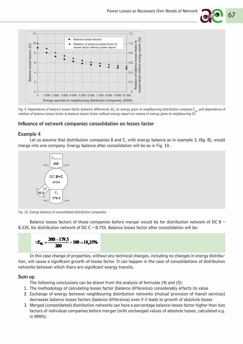
Fig. 9. Dependence of balance losses factor (balance difference) ∆E% on energy given to neighbouring distribution company EoSD and dependence of relation of balance losses factor to balance losses factor without energy export on volume of energy given to neighbouring DC
Influence of network companies consolidation on losses factor
Example 4Let us assume that distribution companies B and C, with energy balance as in example 3, (fig. 8), would
merge into one company. Energy balance after consolidation will be as in Fig. 10..
Fig. 10. Energy balance of consolidated distribution companies
Balance losses factors of those companies before merger would be for distribution network of DC B – 8.33%, for distribution network of DC C – 8.75%. Balance losses factor after consolidation will be:
In this case change of properties, without any technical changes, including no changes in energy distribu-tion, will cause a significant growth of losses factor. It can happen in the case of consolidations of distribution networks between which there are significant energy transits.
Sum upThe following conclusions can be drawn from the analysis of formulas (4) and (5):
1. The methodology of calculating losses factor (balance difference) considerably affects its value2. Exchange of energy between neighbouring distribution networks (mutual provision of transit services)
decreases balance losses factors (balance difference) even if it leads to growth of absolute losses 3. Merged (consolidated) distribution networks can have a percentage balance losses factor higher than loss
factors of individual companies before merger (with unchanged values of absolute losses, calculated e.g. in MWh).
67Power Losses as Necessary Own Needs of Network
13
Fig. 9. Dependence of balance losses factor (balance difference) ΔE% on power energy given to neighbouring distribution company EoSD and dependence of relation of balance losses factor to balance losses factor without power energy export on volume of power energy given to neighbouring SDDC
Influence of network companies consolidation on losses factor Example 4 Let us assume that distribution companies B and C, with power energy balance as
in example 3, (fig. 8), would merge into one company. Power Energy balance after consolidation will be as in Fig. 10.
Fig. 10. Power Energy balance of consolidated distribution companies
ENN/110 200
ES 179.5
ΔE 20.5
DC B+C area
0
2
4
6
8
10
12
0 1 000 2 000 3 000 4 000 5 000 6 000 7 000 8 000 9 000 10 000
Energy exported to neighbouring distribution companies, [GWh]
Bal
ance
loss
es fa
ctor
s, [%
]
0
0.2
0.4
0.6
0.8
1.0
1.2
Rel
atio
n of
bal
ance
loss
es fa
ctor
to
loss
es fa
ctor
with
out e
nerg
y ex
port,
[%]
Balance losses factors
Relation of balance losses factor to losses factor without power export power

3. COMMERCIAL LOSSES As mentioned in chapter 1, commercial losses are caused by errors of measurement systems, errors re-
sulting from sale registration systems and illegal energy consumption.
Errors of measurement systems
Example 5Let us consider the case of a network element, e.g. line with energy measurements at the beginning and at the end. Let us assume that in a certain time period between meters readings, the energy actually transmitted from
the line is 100 kWh; actual energy losses in the line are 0.5 kWh; both meters, at the beginning and the end of the line, are 0.5 class; the meter at the beginning of the line has negative deviation: its indications are by 0.4% lower than the actual energy flow; the meter at the end of the line has a positive deviation: its indications are by 0.3% higher than actual energy volume.
The assumptions indicate the following :• actual energy going to the line is 100.5 kWh• target energy as going to the line is 100.5 – 0.402 ≈ 100.1 kWh• target energy as received from the line is 100 + 0.3 = 100.3 kWh• the difference between the target energy at the beginning and at the end of the line, that is the losses
are: 100.1 – 100.3 = –0.2 kWh.The same example indicates that the balance losses (balance difference) can significantly depend on er-
rors of measurement systems. The error of balance difference is the bigger the smaller the actual losses of the network are.
In practice, the losses analysis refers to network fragments of much bigger losses, from few to over ten percent. But in extreme cases, balance losses (balance difference) can be lower than zero due to errors of measurement systems.
Energy sold registration systemsBigger and more frequent errors can be caused by systems of registration of energy sold. The reports
showing energy sold in reports in individual months can have errors. It refers in particular to the energy sold from LV network. The errors can be due to adoption of e.g. the following rules in meter readings:
1. Meters of energy transmitted to a network are read every month2. Consumers are divided into two groups, e.g. A and B3. In the first group of consumers meters are read in odd months, that is in January, March, May..., and in
the second group - meters are read in even months – that is in February, April, June... 4. The meters readings in each group take one month. Energy consumption in a month is assigned to the
15th day of the given month and is shown as energy consumption in both groups in a given month. So, e.g. energy consumption by consumers of group A, read in the period of in 1st to 31st of January, is as-signed to 15th of January and is indicated in reports as energy consumption by group A and B consumers in January.Considerable differences between the quantity of energy shown in reports as delivered to consumers and
the quantity of energy actually delivered to consumers in individual months can be an effect of “shift of energy consumption readings collection”. As a consequence, the specified balance losses (balance difference) are af-fected by the adopted system of settlement, based on energy consumption forecasts by small retail consum-ers. In relation to actual losses, the values of balance losses (balance difference) are alternately inflated and understated (“waving of losses”).
Example 6Let us consider a simple case in which:
• energy transmitted to the network is read once a month• consumers are divided into two groups A and B, with meter readings every two months. Meters are read
in odd months for group A consumers, and in even months for group B consumers• power consumption by the two groups differs considerably, which can be an effect of random division of
the consumers into those two groups.Let us assume that energy demand and input energy into the network in individual months by all consum-
68Jerzy Kulczycki; Waldemar L. Szpyra/ AGH University of Science and Technology in CracowMichał Rudziński / ENION S.A.
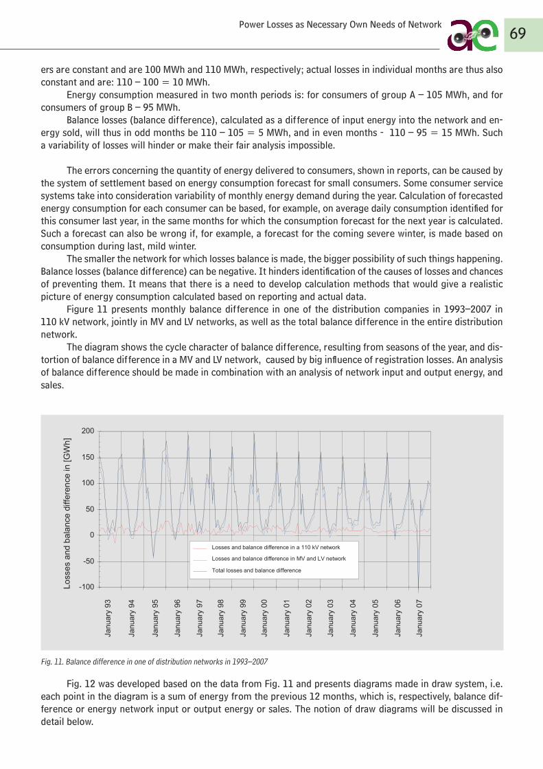
ers are constant and are 100 MWh and 110 MWh, respectively; actual losses in individual months are thus also constant and are: 110 – 100 = 10 MWh.
Energy consumption measured in two month periods is: for consumers of group A – 105 MWh, and for consumers of group B – 95 MWh.
Balance losses (balance difference), calculated as a difference of input energy into the network and en-ergy sold, will thus in odd months be 110 – 105 = 5 MWh, and in even months - 110 – 95 = 15 MWh. Such a variability of losses will hinder or make their fair analysis impossible.
The errors concerning the quantity of energy delivered to consumers, shown in reports, can be caused by the system of settlement based on energy consumption forecast for small consumers. Some consumer service systems take into consideration variability of monthly energy demand during the year. Calculation of forecasted energy consumption for each consumer can be based, for example, on average daily consumption identified for this consumer last year, in the same months for which the consumption forecast for the next year is calculated. Such a forecast can also be wrong if, for example, a forecast for the coming severe winter, is made based on consumption during last, mild winter.
The smaller the network for which losses balance is made, the bigger possibility of such things happening. Balance losses (balance difference) can be negative. It hinders identification of the causes of losses and chances of preventing them. It means that there is a need to develop calculation methods that would give a realistic picture of energy consumption calculated based on reporting and actual data.
Figure 11 presents monthly balance difference in one of the distribution companies in 1993–2007 in 110 kV network, jointly in MV and LV networks, as well as the total balance difference in the entire distribution network.
The diagram shows the cycle character of balance difference, resulting from seasons of the year, and dis-tortion of balance difference in a MV and LV network, caused by big influence of registration losses. An analysis of balance difference should be made in combination with an analysis of network input and output energy, and sales.
Fig. 11. Balance difference in one of distribution networks in 1993–2007
Fig. 12 was developed based on the data from Fig. 11 and presents diagrams made in draw system, i.e. each point in the diagram is a sum of energy from the previous 12 months, which is, respectively, balance dif-ference or energy network input or output energy or sales. The notion of draw diagrams will be discussed in detail below.
69Power Losses as Necessary Own Needs of Network
17
caused by big influence of registration losses. An analysis of balance difference should be made in combination with an analysis of network input and output powerenergy, and sales.
Fig. 11. Balance difference in one of distribution networks in 1993–2007 Fig. 12 was developed based on the data from Fig. 11 and presents diagrams
made in draw system, i.e. each point in the diagram is a sum of power energy from the previous 12 months, which is, respectively, balance difference or power energy network input or output power energy or sales. The notion of draw diagrams will be discussed in detail below.
-100
-50
0
50
100
150
200
Janu
ary
93
Janu
ary
94
Janu
ary
95
Janu
ary
96
Janu
ary
97
Janu
ary
98
Janu
ary
99
Janu
ary
00
Janu
ary
01
Janu
ary
02
Janu
ary
03
Janu
ary
04
Janu
ary
05
Janu
ary
06
Janu
ary
07
Loss
es a
nd b
alan
ce d
iffer
ence
in [G
Wh]
Losses and balance difference in a 110 kV network
Losses and balance difference in MV and LV network Total losses and balance difference
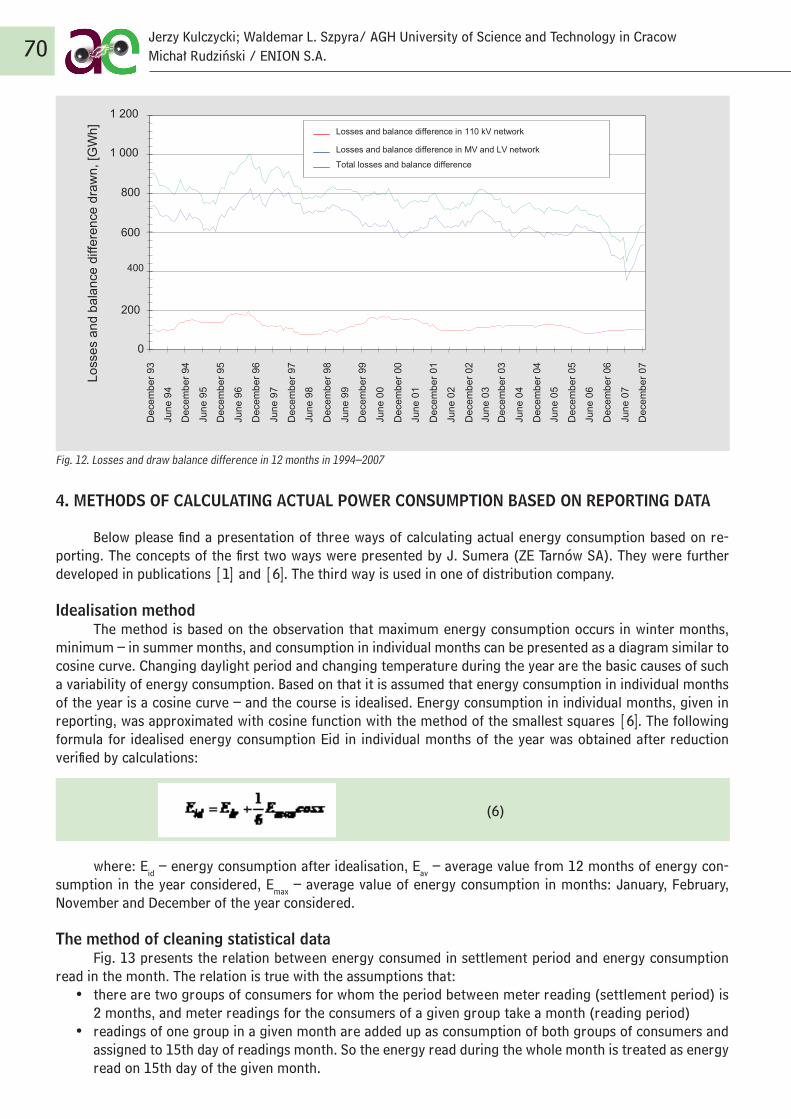
Fig. 12. Losses and draw balance difference in 12 months in 1994–2007
4. METHODS OF CALCULATING ACTUAL POWER CONSUMPTION BASED ON REPORTING DATA
Below please find a presentation of three ways of calculating actual energy consumption based on re-porting. The concepts of the first two ways were presented by J. Sumera (ZE Tarnów SA). They were further developed in publications [1] and [6]. The third way is used in one of distribution company.
Idealisation methodThe method is based on the observation that maximum energy consumption occurs in winter months,
minimum – in summer months, and consumption in individual months can be presented as a diagram similar to cosine curve. Changing daylight period and changing temperature during the year are the basic causes of such a variability of energy consumption. Based on that it is assumed that energy consumption in individual months of the year is a cosine curve – and the course is idealised. Energy consumption in individual months, given in reporting, was approximated with cosine function with the method of the smallest squares [6]. The following formula for idealised energy consumption Eid in individual months of the year was obtained after reduction verified by calculations:
(6)
where: Eid – energy consumption after idealisation, Eav – average value from 12 months of energy con-sumption in the year considered, Emax – average value of energy consumption in months: January, February, November and December of the year considered.
The method of cleaning statistical dataFig. 13 presents the relation between energy consumed in settlement period and energy consumption
read in the month. The relation is true with the assumptions that:• there are two groups of consumers for whom the period between meter reading (settlement period) is
2 months, and meter readings for the consumers of a given group take a month (reading period)• readings of one group in a given month are added up as consumption of both groups of consumers and
assigned to 15th day of readings month. So the energy read during the whole month is treated as energy read on 15th day of the given month.
70Jerzy Kulczycki; Waldemar L. Szpyra/ AGH University of Science and Technology in CracowMichał Rudziński / ENION S.A.
18
Fig. 12. Losses and draw balance difference in 12 months in 1994–2007
Methods of calculating actual power consumption based on reporting data Below please find a presentation of three ways of calculating actual power
energy consumption based on reporting. The concepts of the first two ways were presented by J. Sumera (ZE Tarnów SA). They were further developed in publications [1] and [6]. The third way is used in one of distribution networkscompany.
Idealisation method The method is based on the observation that maximum power energy
consumption occurs in winter months, minimum – in summer months, and consumption in individual months can be presented as a diagram similar to cosine curve. Changing daylight period and changing temperature during the year are the basic causes of such a variability of power energy consumption. Based on that it is assumed that power energy consumption in individual months of the year is a cosine curve – and the course is idealised. Power Energy consumption in individual months, given in reporting, was approximated with cosine function with the method of the smallest squares [6]. The following formula for idealised power energy consumption Eid in individual months of the year was obtained after reduction verified by calculations:
cosxEEE maxavid 61 (6)
0
200
400
600
800
1 000
1 200
Loss
es a
nd b
alan
ce d
iffer
ence
dra
wn,
[GW
h]
Dec
embe
r 93
June
94
Dec
embe
r 94
June
95
Dec
embe
r 95
June
96
Dec
embe
r 96
June
97
Dec
embe
r 97
June
98
Dec
embe
r 98
June
99
Dec
embe
r 99
Dec
embe
r 00
Dec
embe
r 01
June
02
Dec
embe
r 02
June
03
Dec
embe
r 03
June
04
Dec
embe
r 04
June
05
Dec
embe
r 05
June
06
Dec
embe
r 06
June
07
Dec
embe
r 07
June
01
June
00
Losses and balance difference in 110 kV network
Losses and balance difference in MV and LV network
Total losses and balance difference
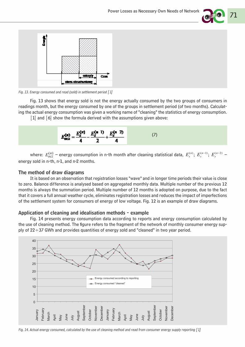
Fig. 13. Energy consumed and read (sold) in settlement period [1]
Fig. 13 shows that energy sold is not the energy actually consumed by the two groups of consumers in readings month, but the energy consumed by one of the groups in settlement period (of two months). Calculat-ing the actual energy consumption was given a working name of “cleaning” the statistics of energy consumption.
[1] and [6] show the formula derived with the assumptions given above:
(7)
where: )(noczE – energy consumption in n-th month after cleaning statistical data, )2()1()( ; ; −− n
sn
sn
s EEE – energy sold in n-th, n-1, and n-2 months.
The method of draw diagramsIt is based on an observation that registration losses “wave” and in longer time periods their value is close
to zero. Balance difference is analysed based on aggregated monthly data. Multiple number of the previous 12 months is always the summation period. Multiple number of 12 months is adopted on purpose, due to the fact that it covers a full annual weather cycle, eliminates registration losses and reduces the impact of imperfections of the settlement system for consumers of energy of low voltage. Fig. 12 is an example of draw diagrams.
Application of cleaning and idealisation methods - exampleFig. 14 presents energy consumption data according to reports and energy consumption calculated by
the use of cleaning method. The figure refers to the fragment of the network of monthly consumer energy sup-ply of 22÷37 GWh and provides quantities of energy sold and “cleaned” in two year period.
Fig. 14. Actual energy consumed, calculated by the use of cleaning method and read from consumer energy supply reporting [1]
71Power Losses as Necessary Own Needs of Network
Fig. 14. Actual energy consumed, calculated by the use of cleaning method and read from consumer energy supply reporting [1] Str. 74 w. 6g jest: Voltage levels of 110 kV in LV stations... Powinno być: Voltage levels of 110 kV in UHV stations... Str. 74 w. 11d (zbędny odstep pomiędzy UHV a znakiem /) jest: Construction of new UHV /110 kV stations Powinno być: Construction of new UHV/110 kV stations Str 75 w. 5g , 7g i 20g (zbędny odstep pomiędzy UHV a znakiem /) jest: UHV /110 kV Powinno być: UHV/110 kV
0 5
10 15 20 25 30 35 40
Nov
embe
r
Dec
embe
r
Janu
ary
Mar
ch
Febr
uary
Apr
il
June
May
July
Aug
ust
Sep
tem
ber
Oct
ober
Nov
embe
r
Dec
embe
r
Janu
ary
Febr
uary
Mar
ch
Apr
il
May
June
July
Sep
tem
ber
Aug
ust
Oct
ober
Month
Ene
rgy,
[GW
h]
Energy consumed according to reporting
Energy consumed “cleaned”
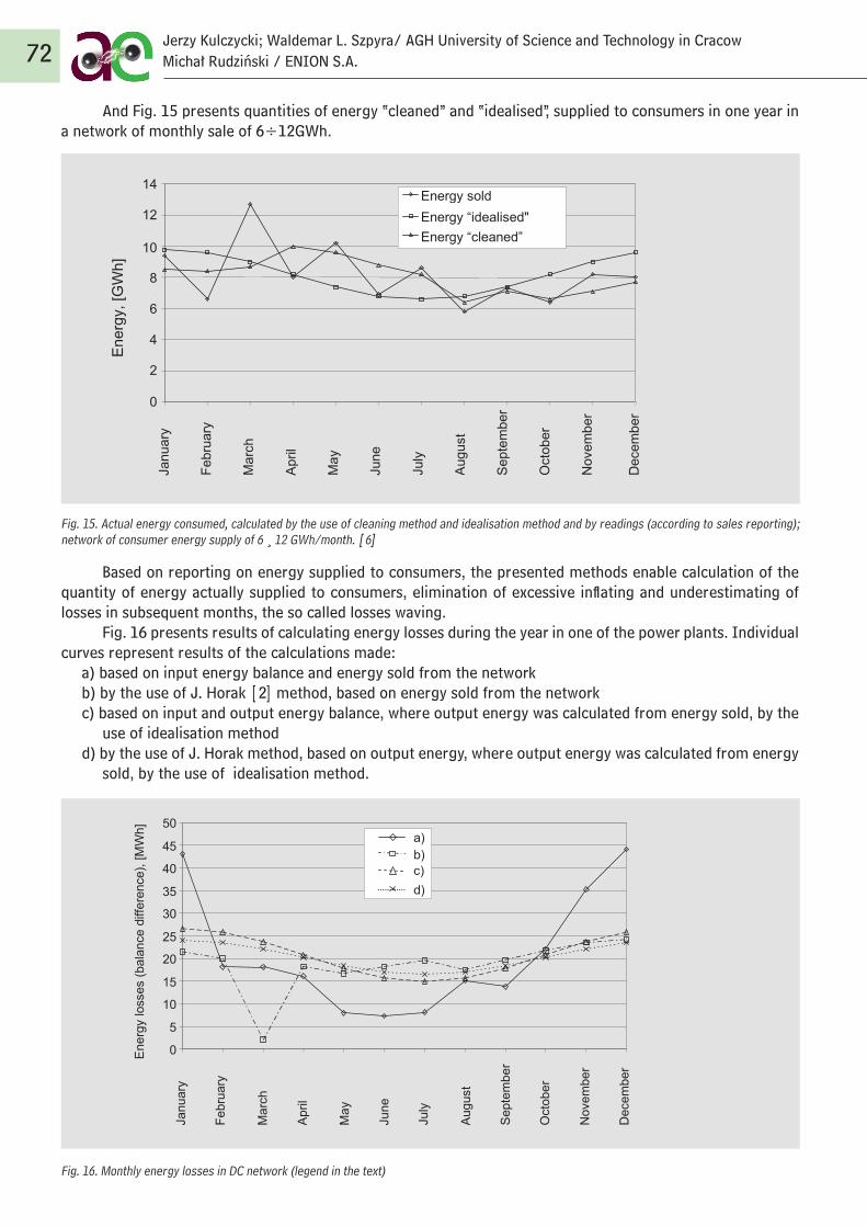
And Fig. 15 presents quantities of energy “cleaned” and “idealised”, supplied to consumers in one year in a network of monthly sale of 6÷12GWh.
Fig. 15. Actual energy consumed, calculated by the use of cleaning method and idealisation method and by readings (according to sales reporting); network of consumer energy supply of 6 ¸ 12 GWh/month. [6]
Based on reporting on energy supplied to consumers, the presented methods enable calculation of the quantity of energy actually supplied to consumers, elimination of excessive inflating and underestimating of losses in subsequent months, the so called losses waving.
Fig. 16 presents results of calculating energy losses during the year in one of the power plants. Individual curves represent results of the calculations made:
a) based on input energy balance and energy sold from the networkb) by the use of J. Horak [2] method, based on energy sold from the networkc) based on input and output energy balance, where output energy was calculated from energy sold, by the
use of idealisation methodd) by the use of J. Horak method, based on output energy, where output energy was calculated from energy
sold, by the use of idealisation method.
Fig. 16. Monthly energy losses in DC network (legend in the text)
72Jerzy Kulczycki; Waldemar L. Szpyra/ AGH University of Science and Technology in CracowMichał Rudziński / ENION S.A.
21
Fig. 15. Actual power energy consumed, calculated by the use of cleaning method and idealisation method and by readings (according to sales reporting); network of consumer power energy supply of 6 12 GWh/month. [6]
Based on reporting on power energy supplied to consumers, the presented
methods enable calculation of the quantity of power energy actually supplied to consumers, elimination of excessive inflating and underestimating of losses in subsequent months, the so called losses waving.
Fig. 16 presents results of calculating power energy losses during the year in one of the power plants. Individual curves represent results of the calculations made: a) based on input power energy balance and power sold from the network b) by the use of J. Horak [2] method, based on power energy sold from the network c) based on input and output power energy balance, where output power energy was
calculated from power energy sold, by the use of idealisation method d) by the use of J. Horak method, based on output powerenergy, where output power
energy was calculated from power energy sold, by the use of idealisation method.
0 2 4 6
8
10
12
14
Janu
ary
Febr
uary
Mar
ch
Apr
il
May
June
July
Aug
ust
Sep
tem
ber
Oct
ober
Nov
embe
r
Dec
embe
r
Month
Ene
rgy,
[GW
h]
Energy sold Energy “idealised" Energy “cleaned”
22
Fig. 16. Monthly power energy losses in DC networkZE (legend in the text)
Sum up Errors of measurement systems, errors resulting from registration systems of
power energy sold and illegal power energy consumption are causes of commercial losses. The value of balance losses (balance difference) is seen in relation to actual losses, and often the values are inflated or underestimated (“losses waving”). It is caused by commercial losses, and in particular by errors resulting from registration systems of power energy sold. In extreme cases, balance difference can be negative.
Three methods of calculating actual power energy consumption and actual losses based on reporting data were presented: idealisation method method of cleaning statistical data method of draw diagrams.
Based on reporting of consumer power energy supplied, the methods enable calculating the power energy actually supplied to consumers and eliminating the effect of “losses waving”.
The following conclusions can be drawn from the applications of the methods presented:
1. There can be significant differences between power energy supplied to consumers and power energy indicated in reportingreports, and the quantity of power energycalculated by the use of these methods
2. The method of draw diagrams and idealisation method are less work consuming than cleaning methods and enable the following calculations:
method of draw diagrams – annual actual losses
0
5
10
15
20
25
30
35
40
45
50
Janu
ary
Febr
uary
Mar
ch
Apr
il
May
June
July
Aug
ust
Sep
tem
ber
Oct
ober
Nov
embe
r
Dec
embe
r
Month
Ene
rgy
loss
es (b
alan
ce d
iffer
ence
), [M
Wh]
a) b) c) d)

Sum upErrors of measurement systems, errors resulting from registration systems of energy sold and illegal
energy consumption are causes of commercial losses. The value of balance losses (balance difference) is seen in relation to actual losses, and often the values are inflated or underestimated (“losses waving”). It is caused by commercial losses, and in particular by errors resulting from registration systems of energy sold. In extreme cases, balance difference can be negative.
Three methods of calculating actual energy consumption and actual losses based on reporting data were presented:
• idealisation method• method of cleaning statistical data• method of draw diagrams.
Based on reporting of consumer energy supplied, the methods enable calculating the energy actually supplied to consumers and eliminating the effect of “losses waving”.
The following conclusions can be drawn from the applications of the methods presented:1. There can be significant differences between energy supplied to consumers and energy indicated in re-
ports, and the quantity of energy calculated by the use of these methods2. The method of draw diagrams and idealisation method are less work consuming than cleaning methods
and enable the following calculations:• method of draw diagrams – annual actual losses • idealisation method – course of actual consumption
3. The cleaning method requires (in comparison with the two other methods) longer calculations based on knowledge of the causes of distortions in meter readings
4. The method of draw diagrams does not have any assumptions concerning the course of energy con-sumption. Idealisation method assumes cosine curve course of monthly energy quantities, and cleaning method assumes that daily energy consumption in a given month is the same. It follows from the analysis of these assumptions that the cleaning method is the most accurate one
5. Comparison of the courses of energy consumption according to reporting and “cleaned” energy indicates that the cleaning method shifts actual energy consumption towards previous months.
Technical losses independent of distribution network operator Decisions of ultra high voltage (UHV) network operator (Area Dispatch Centres) can affect losses in the
fed 110 kV distribution network. The volume of these losses is affected in particular by:1. Power distribution in a UHV network2. Voltage regulation in UHV/110 kV stations3. Decisions on 110 kV network structure. The network is owned by operators of distribution networks, but
the lines that significantly affect power transmitted from power plant or serving to transmit power be-tween companies are coordinated by Area Dispatch Centres
4. Construction of new UHV/110 kV stations.Also contractual obligations resulting from contracts with customers can affect increase of losses in MV
networks. It refers to cut locations in MV networks.
Load flow in a UHV networkChanges in power generation among power plants affect on load flow in UHV network, and consequently,
the load of individual UHV/110 kV stations. Change of these loads leads to change of load flow and power losses in 110 kV network, which is illustrated in figure 17. 110 kV network of a distribution company is fed from two stations of the highest voltage: 220/110 kV station and 400/110 kV station. The figure shows (in relative units) active power flow in UHV lines feeding the stations (the total power coming to 110 kV network via the two stations feeding the network is a reference unit). In normal working conditions, both stations are loaded with active power of 0.5.
If there is a change of power generated in power centres feeding UHV network, power flow in this net-work (values in brackets) will also change considerably. The changes will cause changes of load of LV/110 kV stations (up to 0.2 and 0.8 of reference power, respectively). These changes will result in changes of power flow and losses in the 110 kV network.
73Power Losses as Necessary Own Needs of Network
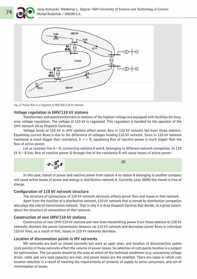
74Jerzy Kulczycki; Waldemar L. Szpyra/ AGH University of Science and Technology in CracowMichał Rudziński / ENION S.A.
Fig. 17. Power flow in a fragment of 400/220/110 kV network
Voltage regulation in UHV/110 kV stationsTransformers and autotransformers in stations of the highest voltage are equipped with facilities for long-
wise voltage regulation. The voltage of 110 kV is regulated. This regulation is handled by the operator of the UHV network (Area Dispatch Centres).
Voltage levels of 110 kV in UHV stations affect power flow in 110 kV network fed from those stations. Equalising current flows is due to the difference of voltages feeding 110 kV network. Since in 110 kV network reactance is much bigger than resistance, X >> R, equalising flow of reactive power is much bigger than the flow of active power.
Let us consider line A – B, connecting stations A and B, belonging to different network companies. In 110 kV A – B line, flow of reactive power Q through line of the resistance R will cause losses of active power:
(8)
In this case, transit of power and reactive power from station A to station B belonging to another company will cause active losses of power and energy in distribution network A. Currently (July 2009) this transit is free of charge.
Configuration of 110 kV network structureThe structure of connections of 110 kV network obviously affects power flow and losses in that network.Apart from the function of a distribution network, 110 kV network that is owned by distribution companies
also plays the role of transmission network. That is why it is Area Dispatch Centres that decide, to a great extent, about the structure of connections of that network.
Construction of new UHV/110 kV stationsConstruction of new UHV/110 kV stations and new lines transmitting power from those stations to 110 kV
networks shortens the power transmission distance via 110 kV network and decreases power flows in individual 110 kV lines; as a result of that, losses in 110 kV networks decrease.
Location of disconnetion points in MV networksMV networks are built as closed networks but work as open ones; and location of disconnection points
(cuts points) of those networks affect the volume of power losses. So selection of cuts points location is a subject for optimisation. The cut points should be the ones at which all the technical conditions (e.g. concerning voltage drops, cable and wire load capacity) are met, and power losses are the smallest. There are cases in which cuts location selection is a result of meeting the requirements of certainty of supply to some consumers, and not of minimisation of losses.
75Power Losses as Necessary Own Needs of Network
Sum upDecisions of UHV network operator and contractual obligations resulting from contracts with some customers
can affect the losses of the fed 110 kV distribution network. The volume of these losses is affected in particular by:• power flow in UHV network• voltage regulation voltage in UHV/110 kV stations• decisions on 110 kV network structure • construction of new UHV/110 kV stations.
Changes in distribution of power generation among power plants affect power flow in the UHV network, and consequently, the load of individual UHV/110 kV stations. Change of these loads leads to change of power flow and power losses in 110 kV network.
This regulation is handled by the operator of the network of the highest voltage.Voltage levels of 110 kV in UHV stations affect power flow in 110 kV network fed from those stations.
Equalising current flows is due to the difference of voltages feeding 110 kV network, and, as a consequence, energy losses.
The structure of connections of 110 kV network obviously affects power flow and losses in that network. 110 kV network is owned by distribution companies, and the lines that significantly affect power output from the power plant or that are used for power transit between distribution networks are coordinated by Area Dis-patch Centres.
By shortening the distance of power transmission via 110 kV network and decreasing power flow in 110 kV lines, construction of new UHV/110 kV stations decreases losses in 110 kV networks.
Taking into consideration the requirements of increased certainty of supply for some consumers can be connected with increase of power losses in networks supplying those consumers.
5. OTHER FACTORS OF NETWORK OPERATION QUALITY
Classification of losses in network and various losses factors used to assess network efficiency were pre-sented in previous chapters. Losses factors cannot, however, be the only basis for assessing a network both for its structure and operation. In market economy, company operation is assessed based on financial indicators, such as liquidity, active participation, profitability and debt ratio.
In electric power distribution companies efficiency measure could be composed of unit costs of power distribution, measured as a quotient of total costs of operation connected with power transmission and distribu-tion and the total quantity of power that was transmitted through the network of the company (supplied to end consumers or neighbouring companies) in a given time period (e.g. in a year). Unit costs of power transmission (distribution) in networks of individual organisational units of the company or at individual voltage levels, or, finally, in individual facilities can also be determined.
One should remember, however, that distribution companies operate in the areas that differ in population density, industrialisation level and land features. These factors significantly affect on a network structure and extent of its use. That is why unit costs of power distribution (and power losses, for that matter) are different in the companies operating in different areas.
Reduction of distribution unit costs is possible by reducing costs and/or increase of the quantity of the power supplied to consumers. Both options are limited, however. Operation of distribution companies is regulated by the Act Energy Law [7] and regulations to that Act, and in particular “tariff” [4] and “system” [5] ordinances. Meeting the requirements of that legislation often leads to investments, and, consequently, to growth of costs.
Reduction of power losses in electric power networks operated by those companies is one of the ways to reduce costs. Losses can be reduced by various operational activities or by investments. Operational ways of losses reduction in distribution networks include, inter alia, voltage regulation in those networks, reducing voltage and current asymmetry and distortion, change of cut points of medium voltage network.
It should also be noted that e.g. in some extreme cases voltage regulation that reduces power and energy losses can reduce the power consumed by consumers, and thus reduce income on transmission charges.

76
LITERATURE
[1] Bogacz S., Więcek M., Estymacja strat energii w wybranym zakładzie energetycznym, diploma thesis. Wydział Ele-ktrotechniki, Automatyki i Elektroniki AGH, Kraków 1996.
[2] Horak J., Gawlak A., Szkutnik J., Sieć elektroenergetyczna jako zbiór elementów. Wydawnictwo Politechniki Częstochowskiej, Częstochowa 1998.
[3] Horak J., Popczyk J., Eksploatacja elektroenergetycznych sieci rozdzielczych. WNT Warszawa 1985.[4] Ordinance of Minister of Economy of 2 July 2007 on detailed principles of development and calculation of tariffs
and settlements in electric power trading (Journal of Laws of 18 July 2007, No 128, pos. 895).[5] Ordinance of Minister of Economy of 4 May 2007 on detailed conditions of electric power system functioning
(Journal of Laws No 93 of 29 May 2007, pos.623).[6] Rutowicz R., Szacunek strat energii w sieciach zakładu energetycznego z uwzględnieniem błędów systemów
sprzedaży, diploma thesis. Faculty of Electrical Engineering, Automatics, IT and Electronics of AGH University of Science and Technology, Cracow 1997.
[7] The Act of 10 April 1997 Energy law (Journal of Laws No 54 pos. 348 with later amendments – Journal of Laws No 158, pos. 1042 and of 1998, No 94 pos. 594 and No 108 pos. 668).
Jerzy Kulczycki; Waldemar L. Szpyra/ AGH University of Science and Technology in CracowMichał Rudziński / ENION S.A.


Zbigniew LubośnyGdańsk / Polska
Zbigniew Lubosny graduated from the Gdansk University of Technology (Poland) in 1985. He received his Ph.D. degree in 1991 and D.Sc. degree in 1999 from the same university. He is currently full Profes-sor (since 2004) at the Gdansk University of Technology and Research Fellow at the University of Edinburgh, UK. His fields of interests include mathematical mod-eling, power system stability and control, artificial intelligence utilization to power system control, wind turbines modeling and control.
Janusz W. BiałekDurham / Wielka Brytania
Janusz W. Bialek holds M.Eng. (1977) and Ph.D. (1981) degrees in Electrical Engine-ering from Warsaw University of Technology (Poland), where he worked from 1981 to 1989. From 1989 to 2002 he was with Uni-versity of Durham, UK. From 2003 to 2009 he held Bert Whittington Chair of Electrical Engineering at the University of Edinburgh, UK. Since 2009 he has held Chair of Electrical Power and Control at Durham University, UK. His research interests are in power system security, liberalization of the electricity power industry, and in power system dynamics.
Authors / Biographies
78Zbigniew Lubośny / Gdansk University of TechnologyJanusz W. Białek / Durham University
Abstract
ANALYTICAL DERIVATION OF PSS PARAMETERSFOR GENERATOR WITH STATIC EXCITATION SYSTEM1
Zbigniew Lubośny / Gdansk University of TechnologyJanusz W. Białek / Durham University
I. NOMENCLATURE
Hjj – inertia constant, Eqj – q-axis steady-state internal emf,Iqj – stator current in the q-axis,K1-K6, T3j – parameters of linear model,KPSS, Ta-Tfj – PSS gain and time constants,Pg, Pref, Qgj – generator real, reference and reactive power,Rt, Xtj – step-up transformer resistance and reactance,Rs, Xsj – system resistance and reactance,Rl, Xlj – armature resistance and leakage reactance,Tg, Tmj – electromagnetic and mechanical torque,Ug, Uref, Usj – terminal, reference and infinite bus voltage,Xad, Xaqj – mutual reactance in d and q-axis,Xaduj – unsaturated mutual reactance in d-axis,X’dj – transient reactance in d-axis,Xfj – field circuit reactance,δ j – power angle,ω, ω0 – rotor speed, synchronous speed.
II. INTRODUCTIONProblem of damping electromechanical oscillations in electric power systems is not new. Since the 1950s,
when power systems started to get bigger and ever more stressed, engineers have been looking for synchro-nous generator controllers that could improve damping of oscillations.
The most popular tool for power system stability enhancement is the power system stabilizer (PSS) which provides an auxiliary control loop to the main automatic voltage regulator (AVR). PSS structure usually follows one of IEEE standards [1]. PSSs are usually of the single-input type with constant parameters (time-invariant) but two-input stabilizers are used too. PSS design is usually based on the compensation of plant frequency characteristics, optimization of defined quality indices, or shifting poles of the considered system to appropri-ate locations.
1 This work was supported by the Engineering and Physical Sciences Research Council, grant GR/S28082/01 “SUPERGEN: Future Network Tech-nologies”. .
Analytical derivation of pss parametersFor generator with static excitation system 79
This paper presents a methodology for PSS design which results in a PSS producing a nearly pure damping torque component in a wide frequency range. The derivation is based on the Heffron-Phillips single-machine infinite-bus-bar model and for a generator with static exciter and speed-based PSS. The choice of time constants is very simple and the only parameter still to be optimized is the PSS gain. Effectiveness of the PSS has been confirmed by tests con-ducted on single- and multi-machine power system model.
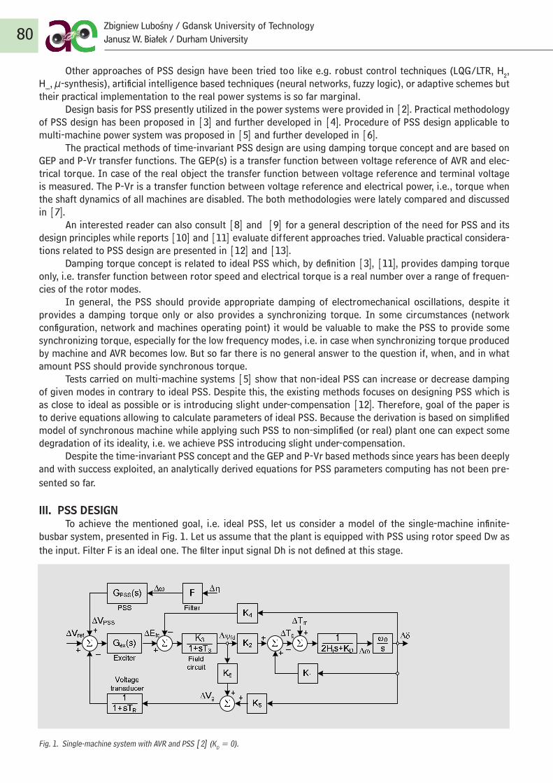
Other approaches of PSS design have been tried too like e.g. robust control techniques (LQG/LTR, H2, H∞, µ-synthesis), artificial intelligence based techniques (neural networks, fuzzy logic), or adaptive schemes but their practical implementation to the real power systems is so far marginal.
Design basis for PSS presently utilized in the power systems were provided in [2]. Practical methodology of PSS design has been proposed in [3] and further developed in [4]. Procedure of PSS design applicable to multi-machine power system was proposed in [5] and further developed in [6].
The practical methods of time-invariant PSS design are using damping torque concept and are based on GEP and P-Vr transfer functions. The GEP(s) is a transfer function between voltage reference of AVR and elec-trical torque. In case of the real object the transfer function between voltage reference and terminal voltage is measured. The P-Vr is a transfer function between voltage reference and electrical power, i.e., torque when the shaft dynamics of all machines are disabled. The both methodologies were lately compared and discussed in [7].
An interested reader can also consult [8] and [9] for a general description of the need for PSS and its design principles while reports [10] and [11] evaluate different approaches tried. Valuable practical considera-tions related to PSS design are presented in [12] and [13].
Damping torque concept is related to ideal PSS which, by definition [3], [11], provides damping torque only, i.e. transfer function between rotor speed and electrical torque is a real number over a range of frequen-cies of the rotor modes.
In general, the PSS should provide appropriate damping of electromechanical oscillations, despite it provides a damping torque only or also provides a synchronizing torque. In some circumstances (network configuration, network and machines operating point) it would be valuable to make the PSS to provide some synchronizing torque, especially for the low frequency modes, i.e. in case when synchronizing torque produced by machine and AVR becomes low. But so far there is no general answer to the question if, when, and in what amount PSS should provide synchronous torque.
Tests carried on multi-machine systems [5] show that non-ideal PSS can increase or decrease damping of given modes in contrary to ideal PSS. Despite this, the existing methods focuses on designing PSS which is as close to ideal as possible or is introducing slight under-compensation [12]. Therefore, goal of the paper is to derive equations allowing to calculate parameters of ideal PSS. Because the derivation is based on simplified model of synchronous machine while applying such PSS to non-simplified (or real) plant one can expect some degradation of its ideality, i.e. we achieve PSS introducing slight under-compensation.
Despite the time-invariant PSS concept and the GEP and P-Vr based methods since years has been deeply and with success exploited, an analytically derived equations for PSS parameters computing has not been pre-sented so far.
III. PSS DESIGNTo achieve the mentioned goal, i.e. ideal PSS, let us consider a model of the single-machine infinite-
busbar system, presented in Fig. 1. Let us assume that the plant is equipped with PSS using rotor speed Dw as the input. Filter F is an ideal one. The filter input signal Dh is not defined at this stage.
Fig. 1. Single-machine system with AVR and PSS [2] (KD = 0).
80Zbigniew Lubośny / Gdansk University of TechnologyJanusz W. Białek / Durham University
2
PSS to non-simplified (or real) plant one can expect some degradation of its ideality, i.e. we achieve PSS introducing slight under-compensation.
Despite the time-invariant PSS concept and the GEP and P-Vr based methods since years has been deeply and with success exploited, an analytically derived equations for PSS parameters computing has not been presented so far.
III. PSS DESIGN
To achieve the mentioned goal, i.e. ideal PSS, let us consider a model of the single-machine infinite-busbar system, presented in Fig. 1. Let us assume that the plant is equipped with PSS using rotor speed ∆ω as the input. Filter F is an ideal one. The filter input signal ∆η is not defined at this stage.
Fig. 1. Single-machine system with AVR and PSS [2] (KD = 0).
The electromagnetic torque ∆Tg can be defined as a function of the rotor angle ∆δ, the reference voltage ∆Vref and the rotor speed ∆ω :
ωδδ ∆⋅+∆⋅+∆⋅=∆ )()()( sTVsTsTT PSSrefVg (1)
where Tδ(s), TV(s), TPSS(s) are some transfer functions that depend on the plant’s parameters K1-K6, T3 and on the controller’s transfer functions, defined by Gex(s) and GPSS(s). What is important here, the PSS transfer function GPSS(s)appears in the TPSS(s) transfer function only.
The electromagnetic torque produced by the PSS is equal to:
ωω ∆+++
+=∆⋅=∆)()1)(1(
)1)(()()(633
32sGKKsTsT
sTsGsGKKsTTexR
RPSSexPSSPSS (2)
After introducing the PSS and the AVR transfer functions to (2) the TPSS(s) function can be written in form:
Ksb
saKsT M
j
jj
N
i
ii
PSSPSS =∑+
∑+=
=
=
1
1
1
1)( (3)
The electromagnetic torque ∆TPSS produced by the PSS will be in phase with the rotor speed ∆ω, i.e. we will achieve the ideal power system stabilizer, when the transfer function TPSS(s) will become real.
The function (3) takes form of a gain K when, for example, the following requirement is fulfilled:
iiMNNiba =∀
== ,...1 (4)
i.e. the numerator and the denominator coefficients, located at the same positions, are equal to each other. When this requirement is fulfilled the PSS is providing the damping torque only for the all frequencies of oscillations.
The search for such PSS means deriving formulas defining the PSS parameters that fulfill requirement (4). To find an analytical solution to the problem it is necessary to make some initial assumptions, i.e.: • allow the PSS’s numerator rank to be higher than the
denominator rank, • allow the AVR parameters to be defined by the derived
equations, • neglect dynamics of some components with small time
constant, e.g. voltage transducer.
To verify the proposed method let us consider a static excitation system (IEEE ST1A model), presented in Fig. 2.
Fig. 2. IEEE type ST1A static excitation system
Let us assume also that the initial transfer function of the PSS is as follows:
d
cbaPSSPSS sT
sTsTsTKsG+
+++=1
)1)(1)(1()( (5)
Additionally, let us neglect the voltage transducer dynamics, by assuming that TR = 0.
For a such defined plant the parameters of the PSS that provides damping torque only are defined by (6):
Aa TT = , Bb TT = , A
Fc KKK
TT631 +
= , Fd TT = (6)
Simultaneously, some of the AVR parameters have to be defined as follow:
3TTC = , 3
63 TTTKKK BA
F = , 3TTTTTT BA
BAF −+= (7)
The Eqs. (6) and (7) define the ideal PSS of a given structure.
Gain K which is a measure of the damping torque provided by the PSS, is here equal to:
A
PSSAKKK
KKKKK63
321 +
= (8)
In the real power systems the AVR, presented in Fig. 2, is also (even often) utilized in one of the following form: • with existing feedback loop (KF ≠ 0) but without transient
gain reduction block (TGR) (TB = TC), • with existing transient gain reduction block (TB ≠ TC) but
without feedback loop (KF = 0). In the first case, i.e. for synchronous generator equipped
with AVR without TGR the PSS and AVR parameters are
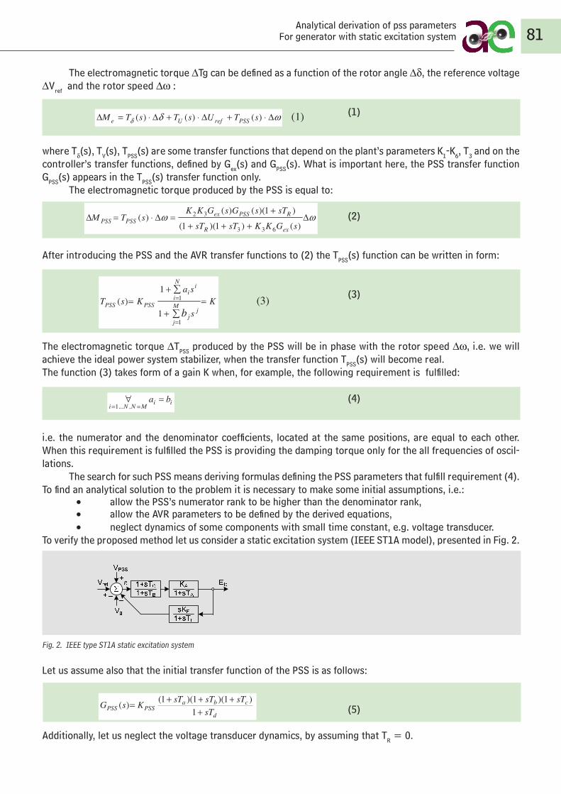
The electromagnetic torque ∆Tg can be defined as a function of the rotor angle ∆δ, the reference voltage ∆Vref and the rotor speed ∆ω : (1)
where Tδ(s), TV(s), TPSS(s) are some transfer functions that depend on the plant’s parameters K1-K6, T3 and on the controller’s transfer functions, defined by Gex(s) and GPSS(s). What is important here, the PSS transfer function GPSS(s) appears in the TPSS(s) transfer function only.
The electromagnetic torque produced by the PSS is equal to:
(2)
After introducing the PSS and the AVR transfer functions to (2) the TPSS(s) function can be written in form:
(3)
The electromagnetic torque ∆TPSS produced by the PSS will be in phase with the rotor speed ∆ω, i.e. we will achieve the ideal power system stabilizer, when the transfer function TPSS(s) will become real. The function (3) takes form of a gain K when, for example, the following requirement is fulfilled:
(4)
i.e. the numerator and the denominator coefficients, located at the same positions, are equal to each other. When this requirement is fulfilled the PSS is providing the damping torque only for the all frequencies of oscil-lations.
The search for such PSS means deriving formulas defining the PSS parameters that fulfill requirement (4). To find an analytical solution to the problem it is necessary to make some initial assumptions, i.e.: • allow the PSS’s numerator rank to be higher than the denominator rank, • allow the AVR parameters to be defined by the derived equations, • neglect dynamics of some components with small time constant, e.g. voltage transducer.To verify the proposed method let us consider a static excitation system (IEEE ST1A model), presented in Fig. 2.
Fig. 2. IEEE type ST1A static excitation system
Let us assume also that the initial transfer function of the PSS is as follows:
(5)
Additionally, let us neglect the voltage transducer dynamics, by assuming that TR = 0.
81Analytical derivation of pss parameters
For generator with static excitation system
4
Rys. 1. Liniowy model układu jednomaszynowego z regulatorem napięcia (RN) i stabilizatorem syste-
mowym (PSS), (KD = 0)
Moment elektromagnetyczny ∆Me moŜna zdefiniować jako funkcję kąta mocy ∆δ, napięcia zadanego
generatora ∆Vref oraz prędkości kątowej wirnika generatora ∆ω :
ωδδ ∆⋅+∆⋅+∆⋅=∆ )()()( sTUsTsTM PSSrefUe (1)
gdzie Tδ(s), TU(s), TPSS(s) są pewnymi transmitancjami zaleŜnymi od parametrów obiektu K1-K6, T3 oraz od
transmitancji regulatora napięcia generatora synchronicznego Gex(s) oraz transmitancji stabilizatora
systemowego GPSS(s). Co istotne, transmitancja stabilizatora systemowego GPSS(s) występuje tylko w
funkcji TPSS(s).
Moment elektromagnetyczny wytwarzany przez stabilizator systemowy jest równy:
ωω ∆+++
+=∆⋅=∆
)()1)(1(
)1)(()()(
633
32
sGKKsTsT
sTsGsGKKsTM
exR
RPSSexPSSPSS (2)
Po uwzględnieniu w zaleŜności (2) transmitancji stabilizatora systemowego i regulatora napięcia
generatora synchronicznego, transmitancję TPSS(s) (zaleŜność 2) moŜna przedstawić w postaci:
Ks
saKsT M
j
jj
N
i
ii
PSSPSSb
=+
+=
∑
∑
=
=
1
1
1
1)( (3)
Moment (fazor momentu) elektromagnetyczny ∆TPSS, wytwarzany przez stabilizator systemowy PSS,
będzie w fazie z prędkością (fazorem prędkości) wirnika generatora ∆ω, tzn. uzyskamy idealny stabilizator
systemowy, gdy transmitancja TPSS(s) będzie liczbą lub funkcją rzeczywistą.
ZaleŜność (3) staje się równa liczbie rzeczywistej K, gdy np. spełniona jest następująca zaleŜność:
5
iiMNNiba =∀
== ,...1 (4)
tzn. gdy współczynniki wielomianu licznika i mianownika transmitancji (3), znajdujące się na tych samych
pozycjach w wielomianach, będą sobie równe. Spełnienie warunku (4) powoduje, Ŝe rozwaŜany
stabilizator systemowy będzie wytwarzał tylko moment tłumiący o stałej, tj. niezaleŜnej od częstotliwości
wartości, dla dowolnej częstotliwości kołysań elektromechanicznych.
Synteza rozwaŜanego tu stabilizatora systemowego sprowadza się zatem do określenia parametrów
stabilizatora, które spełniają warunek (4).
W celu analitycznego rozwiązania problemu naleŜy przyjąć dodatkowe załoŜenia, a w tym:
• dopuścić rząd wielomianu licznika wyŜszy niŜ wielomianu mianownika transmitancji
• dopuścić moŜliwość definiowania parametrów regulatora napięcia generatora przez wyprowadzone
zaleŜności, tj. w celu spełnienia warunku (4)
• pominąć elementy modelu obiektu o małych stałych czasowych, np. przetwornika pomiarowego
napięcia generatora.
W celu weryfikacji zaproponowanej metody syntezy stabilizatora systemowego przyjmijmy, Ŝe generator
synchroniczny wyposaŜony jest w statyczny układ wzbudzenia i regulacji napięcia typu IEEE ST1A, tj. jak
przedstawiony na rys. 2.
Rys. 2. Model statycznego układu wzbudzenia i regulacji napięcia typu IEEE ST1A
ZałóŜmy wstępnie transmitancję stabilizatora systemowego o postaci jak (5):
d
cbaPSSPSS sT
sTsTsTKsG+
+++=1
)1)(1)(1()( (5)
Ponadto pomińmy dynamikę przetwornika pomiarowego napięcia generatora, przyjmując TR = 0.
Dla tak zdefiniowanego obiektu parametry stabilizatora systemowego wytwarzającego tylko moment
tłumiący określone są następującymi zaleŜnościami:
Aa TT = , Bb TT = , A
Fc KKK
TT631 +
= , Fd TT = (6)
Równocześnie pewne parametry regulatora napięcia generatora muszą być równe:
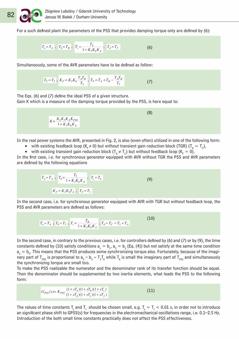
For a such defined plant the parameters of the PSS that provides damping torque only are defined by (6):
(6)
Simultaneously, some of the AVR parameters have to be defined as follow:
(7)
The Eqs. (6) and (7) define the ideal PSS of a given structure.Gain K which is a measure of the damping torque provided by the PSS, is here equal to:
(8)
In the real power systems the AVR, presented in Fig. 2, is also (even often) utilized in one of the following form: • with existing feedback loop (KF ≠ 0) but without transient gain reduction block (TGR) (TB = TC), • with existing transient gain reduction block (TB ≠ TC) but without feedback loop (KF = 0).In the first case, i.e. for synchronous generator equipped with AVR without TGR the PSS and AVR parameters are defined by the following equations
(9)
In the second case, i.e. for synchronous generator equipped with AVR with TGR but without feedback loop, the PSS and AVR parameters are defined as follows:
(10)
In the second case, in contrary to the previous cases, i.e. for controllers defined by (6) and (7) or by (9), the time constants defined by (10) satisfy conditions a1 = b1, a3 = b3 (Eq. (4)) but not satisfy at the same time condition a2 = b2. This means that the PSS produces some synchronizing torque also. Fortunately, because of the imagi-nary part of TPSS is proportional to a2 – b2 ≈ T3TA while TA is small the imaginary part of TPSS and simultaneously the synchronizing torque are small too. To make the PSS realizable the numerator and the denominator rank of its transfer function should be equal. Then the denominator should be supplemented by two inertia elements, what leads the PSS to the following form:
(11)
The values of time constants Te and Tf should be chosen small, e.g. Te = Tf < 0.01 s, in order not to introduce an significant phase shift to GPSS(s) for frequencies in the electromechanical oscillations range, i.e. 0.1–2.5 Hz. Introduction of the both small time constants practically does not affect the PSS effectiveness.
82Zbigniew Lubośny / Gdansk University of TechnologyJanusz W. Białek / Durham University
6
3TTC = , 3
63 TTTKKK BA
F = , 3TTTTTT BA
BAF −+= (7)
Wówczas zaleŜności (6) i (7) definiują tzw. idealny stabilizator systemowy.
Współczynnik K, będący miarą momentu tłumiącego wytwarzanego przez stabilizator systemowy, jest
wówczas równy:
A
PSSA
KKKKKKKK63
321+
= (8)
W rzeczywistości regulator napięcia generatora synchronicznego z rys. 2 dość często występuje w jednej z
następujących postaci (struktur):
• z pętlą sprzęŜenia zwrotnego (KF ≠ 0) ale bez bloku TGR (Transient Reduction Gain) (TB = TC)
• z blokiem TGR (TB ≠ TC), ale bez pętli sprzęŜenia zwrotnego (KF = 0).
W pierwszym przypadku, tj. dla generatora synchronicznego z regulatorem napięcia generatora bez bloku
TGR w swojej strukturze, parametry stabilizatora systemowego i regulatora napięcia definiują następujące
zaleŜności:
Aa TT = , A
b KKKTT
63
31 +
= , dc TT = (9)
AF TKKK 63= , 3TTF =
W drugim przypadku, tj. dla generatora synchronicznego z regulatorem napięcia generatora z blokiem TGR
w swojej strukturze parametry stabilizatora systemowego i regulatora napięcia definiują zaleŜności:
Aa TT = , 3TTb = , A
Bc KKK
TT631 +
= , ACd TTTT +== 3 (10)
W przypadku drugim, w porównaniu z pierwszym, tj. dla regulatorów definiowanych przez zaleŜności (6) i
(7) oraz przez (9), stałe czasowe definiowane zaleŜnością (10) prowadzą do spełniania warunków a1 = b1,
a3 = b3 [zaleŜność (4)], ale nie umoŜliwiają spełnienia warunku a2 = b2. Oznacza to, Ŝe tak określony
stabilizator systemowy wytwarza równieŜ, oprócz momentu tłumiącego, pewien moment synchronizujący.
PoniewaŜ jednak część urojona transmitancji TPSS jest proporcjonalna do a2 - b2 ≈ T3TA, gdzie wartość TA
jest mała, urojona część transmitancji TPSS i równocześnie moment synchronizujący są równieŜ małe.
W celu uzyskania realizowalności stabilizatora systemowego rząd wielomianu licznika jego transmitancji
nie moŜe być większy od rzędu wielomianu mianownika. Aby to uzyskać, tj. doprowadzić do stanu, w
którym rząd wielomianu licznika i mianownika transmitancji stabilizatora systemowego będą równe,
naleŜy uzupełnić mianownik transmitancji z zaleŜności (5) do postaci jak poniŜej:
7
)1)(1)(1()1)(1)(1()(
fed
cbaPSSPSS sTsTsT
sTsTsTKsG++++++= (11)
Wartości stałych czasowych Te i Tf powinny być na tyle małe, np. Te = Tf < 0,01 s, aby w transmitancji
GPSS(s) nie powodować znaczącego przesunięcia fazy z zakresu częstotliwości odpowiadających
częstotliwościom kołysań elektromechanicznych w systemie elektroenergetycznym, tj. 0,1–2,5 Hz.
PowyŜsza modyfikacja transmitancji stabilizatora systemowego praktycznie nie zmniejsza efektywności
rozwaŜanego stabilizatora systemowego.
Wyprowadzone zaleŜności pozwalają na sformułowanie następujących uwag:
• Parametry stabilizatora systemowego i regulatora napięcia generatora definiowane przez powyŜsze
zaleŜności, pozwalające stabilizatorowi systemowemu wytwarzać tylko moment tłumiący, zaleŜą od
punktu pracy generatora synchronicznego, parametrów maszyny i impedancji zewnętrznej (widzianej z
szyn generatora synchronicznego).
• PowyŜsze zaleŜności związane są z eliminowaniem się zer i biegunów transmitancji. Przykładowo,
pewne stałe czasowe w liczniku transmitancji stabilizatora systemowego są równe stałym czasowym
mianownika regulatora napięcia lub obwodu wzbudzenia maszyny (i odwrotnie). Sposób określania
niektórych stałych czasowych wydaje się intuicyjny, podczas gdy sposób definiowania innych stałych
czasowych i współczynnika wzmocnienia w pętli sprzęŜenia zwrotnego nie jest juŜ tak oczywisty.
• ZaleŜności (7), (9) i (10) określają wartości niektórych parametrów regulatora napięcia, które pozwalają
stabilizatorowi systemowemu PSS na optymalność. PowyŜsze, tj. konieczność modyfikacji wartości
nastaw regulatora napięcia, moŜe być traktowane jako ograniczenie proponowanej metody. NaleŜy
jednak podkreślić, Ŝe wartości parametrów regulatora napięcia, obliczone za pomocą powyŜszych
zaleŜności, często są bliskie nastawianym w regulatorach rzeczywistych. Parametry regulatora napięcia
generatora, określone przez zaleŜności (7), (9) oraz (10), pozwalają na poprawną pracę generatora
synchronicznego równieŜ po wyłączeniu stabilizatora systemowego oraz jego wydzieleniu się z pracy w
systemie elektroenergetycznym.
W przypadku regulatora napięcia bez pętli sprzęŜenia zwrotnego własności dynamiczne obiektu mogą
być niezaleŜnie kształtowane przez parametry KA i TB, które nie są definiowane przez zaproponowane
zaleŜności. W przypadku regulatora napięcia z pętlą sprzęŜenia zwrotnego, ale bez bloku TGR,
własności dynamiczne obiektu mogą być niezaleŜnie kształtowane tylko za pomocą współczynnika
wzmocnienia KA, a własności dynamiczne obiektu pracującego poza systemem elektroenergetycznym
(w tym na potrzeby własne) względnie silnie zaleŜą od stałej czasowej TA. Im mniejsza jest jej wartość,
tym lepsze własności dynamiczne obiektu.
• Wartości stałych czasowych stabilizatora systemowego zaleŜą od wartości parametrów regulatora
5
iiMNNiba =∀
== ,...1 (4)
tzn. gdy współczynniki wielomianu licznika i mianownika transmitancji (3), znajdujące się na tych samych
pozycjach w wielomianach, będą sobie równe. Spełnienie warunku (4) powoduje, Ŝe rozwaŜany
stabilizator systemowy będzie wytwarzał tylko moment tłumiący o stałej, tj. niezaleŜnej od częstotliwości
wartości, dla dowolnej częstotliwości kołysań elektromechanicznych.
Synteza rozwaŜanego tu stabilizatora systemowego sprowadza się zatem do określenia parametrów
stabilizatora, które spełniają warunek (4).
W celu analitycznego rozwiązania problemu naleŜy przyjąć dodatkowe załoŜenia, a w tym:
• dopuścić rząd wielomianu licznika wyŜszy niŜ wielomianu mianownika transmitancji
• dopuścić moŜliwość definiowania parametrów regulatora napięcia generatora przez wyprowadzone
zaleŜności, tj. w celu spełnienia warunku (4)
• pominąć elementy modelu obiektu o małych stałych czasowych, np. przetwornika pomiarowego
napięcia generatora.
W celu weryfikacji zaproponowanej metody syntezy stabilizatora systemowego przyjmijmy, Ŝe generator
synchroniczny wyposaŜony jest w statyczny układ wzbudzenia i regulacji napięcia typu IEEE ST1A, tj. jak
przedstawiony na rys. 2.
Rys. 2. Model statycznego układu wzbudzenia i regulacji napięcia typu IEEE ST1A
ZałóŜmy wstępnie transmitancję stabilizatora systemowego o postaci jak (5):
d
cbaPSSPSS sT
sTsTsTKsG+
+++=1
)1)(1)(1()( (5)
Ponadto pomińmy dynamikę przetwornika pomiarowego napięcia generatora, przyjmując TR = 0.
Dla tak zdefiniowanego obiektu parametry stabilizatora systemowego wytwarzającego tylko moment
tłumiący określone są następującymi zaleŜnościami:
Aa TT = , Bb TT = , A
Fc KKK
TT631 +
= , Fd TT = (6)
Równocześnie pewne parametry regulatora napięcia generatora muszą być równe:
6
3TTC = , 3
63 TTTKKK BA
F = , 3TTTTTT BA
BAF −+= (7)
Wówczas zaleŜności (6) i (7) definiują tzw. idealny stabilizator systemowy.
Współczynnik K, będący miarą momentu tłumiącego wytwarzanego przez stabilizator systemowy, jest
wówczas równy:
A
PSSA
KKKKKKKK63
321+
= (8)
W rzeczywistości regulator napięcia generatora synchronicznego z rys. 2 dość często występuje w jednej z
następujących postaci (struktur):
• z pętlą sprzęŜenia zwrotnego (KF ≠ 0) ale bez bloku TGR (Transient Reduction Gain) (TB = TC)
• z blokiem TGR (TB ≠ TC), ale bez pętli sprzęŜenia zwrotnego (KF = 0).
W pierwszym przypadku, tj. dla generatora synchronicznego z regulatorem napięcia generatora bez bloku
TGR w swojej strukturze, parametry stabilizatora systemowego i regulatora napięcia definiują następujące
zaleŜności:
Aa TT = , A
b KKKTT
63
31 +
= , dc TT = (9)
AF TKKK 63= , 3TTF =
W drugim przypadku, tj. dla generatora synchronicznego z regulatorem napięcia generatora z blokiem TGR
w swojej strukturze parametry stabilizatora systemowego i regulatora napięcia definiują zaleŜności:
Aa TT = , 3TTb = , A
Bc KKK
TT631 +
= , ACd TTTT +== 3 (10)
W przypadku drugim, w porównaniu z pierwszym, tj. dla regulatorów definiowanych przez zaleŜności (6) i
(7) oraz przez (9), stałe czasowe definiowane zaleŜnością (10) prowadzą do spełniania warunków a1 = b1,
a3 = b3 [zaleŜność (4)], ale nie umoŜliwiają spełnienia warunku a2 = b2. Oznacza to, Ŝe tak określony
stabilizator systemowy wytwarza równieŜ, oprócz momentu tłumiącego, pewien moment synchronizujący.
PoniewaŜ jednak część urojona transmitancji TPSS jest proporcjonalna do a2 - b2 ≈ T3TA, gdzie wartość TA
jest mała, urojona część transmitancji TPSS i równocześnie moment synchronizujący są równieŜ małe.
W celu uzyskania realizowalności stabilizatora systemowego rząd wielomianu licznika jego transmitancji
nie moŜe być większy od rzędu wielomianu mianownika. Aby to uzyskać, tj. doprowadzić do stanu, w
którym rząd wielomianu licznika i mianownika transmitancji stabilizatora systemowego będą równe,
naleŜy uzupełnić mianownik transmitancji z zaleŜności (5) do postaci jak poniŜej:
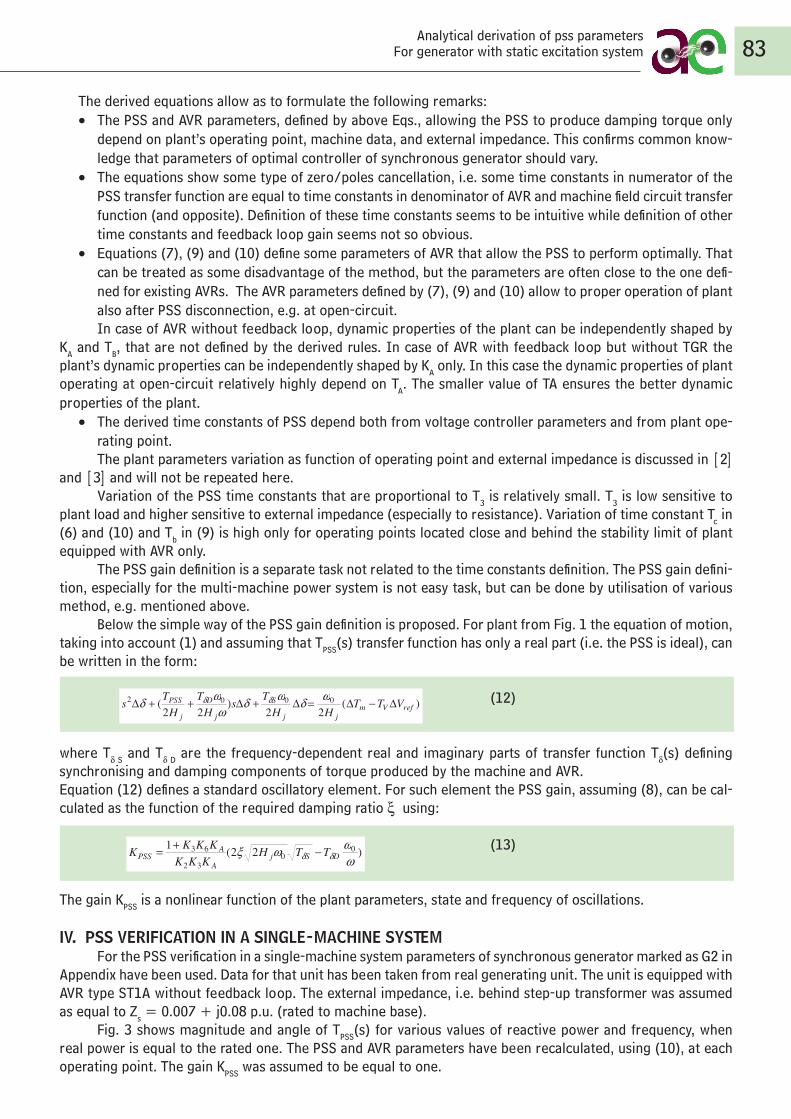
The derived equations allow as to formulate the following remarks:• The PSS and AVR parameters, defined by above Eqs., allowing the PSS to produce damping torque only
depend on plant’s operating point, machine data, and external impedance. This confirms common know-ledge that parameters of optimal controller of synchronous generator should vary.
• The equations show some type of zero/poles cancellation, i.e. some time constants in numerator of the PSS transfer function are equal to time constants in denominator of AVR and machine field circuit transfer function (and opposite). Definition of these time constants seems to be intuitive while definition of other time constants and feedback loop gain seems not so obvious.
• Equations (7), (9) and (10) define some parameters of AVR that allow the PSS to perform optimally. That can be treated as some disadvantage of the method, but the parameters are often close to the one defi-ned for existing AVRs. The AVR parameters defined by (7), (9) and (10) allow to proper operation of plant also after PSS disconnection, e.g. at open-circuit.In case of AVR without feedback loop, dynamic properties of the plant can be independently shaped by
KA and TB, that are not defined by the derived rules. In case of AVR with feedback loop but without TGR the plant’s dynamic properties can be independently shaped by KA only. In this case the dynamic properties of plant operating at open-circuit relatively highly depend on TA. The smaller value of TA ensures the better dynamic properties of the plant.
• The derived time constants of PSS depend both from voltage controller parameters and from plant ope-rating point. The plant parameters variation as function of operating point and external impedance is discussed in [2]
and [3] and will not be repeated here. Variation of the PSS time constants that are proportional to T3 is relatively small. T3 is low sensitive to
plant load and higher sensitive to external impedance (especially to resistance). Variation of time constant Tc in (6) and (10) and Tb in (9) is high only for operating points located close and behind the stability limit of plant equipped with AVR only.
The PSS gain definition is a separate task not related to the time constants definition. The PSS gain defini-tion, especially for the multi-machine power system is not easy task, but can be done by utilisation of various method, e.g. mentioned above.
Below the simple way of the PSS gain definition is proposed. For plant from Fig. 1 the equation of motion, taking into account (1) and assuming that TPSS(s) transfer function has only a real part (i.e. the PSS is ideal), can be written in the form:
(12)
where Tδ S and Tδ D are the frequency-dependent real and imaginary parts of transfer function Tδ(s) defining synchronising and damping components of torque produced by the machine and AVR.Equation (12) defines a standard oscillatory element. For such element the PSS gain, assuming (8), can be cal-culated as the function of the required damping ratio ξ using:
(13)
The gain KPSS is a nonlinear function of the plant parameters, state and frequency of oscillations.
IV. PSS VERIFICATION IN A SINGLE-MACHINE SYSTEMFor the PSS verification in a single-machine system parameters of synchronous generator marked as G2 in
Appendix have been used. Data for that unit has been taken from real generating unit. The unit is equipped with AVR type ST1A without feedback loop. The external impedance, i.e. behind step-up transformer was assumed as equal to Zs = 0.007 + j0.08 p.u. (rated to machine base).
Fig. 3 shows magnitude and angle of TPSS(s) for various values of reactive power and frequency, when real power is equal to the rated one. The PSS and AVR parameters have been recalculated, using (10), at each operating point. The gain KPSS was assumed to be equal to one.
83Analytical derivation of pss parameters
For generator with static excitation system
8
napięcia generatora oraz od stanu pracy generatora.
Zmienność parametrów obiektu (współczynników K1-K6) w funkcji zmienności punktu pracy generatora
i wartości impedancji zewnętrznej jest dyskutowana w pracach [2] i [3] i nie będzie tu powtarzana.
Zmienność stałych czasowych stabilizatora systemowego w funkcji stałej czasowej obiektu T3 jest
względnie mała. Stała czasowa T3 jest mało wraŜliwa na punkt pracy generatora i bardziej wraŜliwa na
wartość impedancji (szczególnie rezystancji) zewnętrznej. Zmienność stałej czasowej Tc w zaleŜności
(6) i (10) oraz stałej czasowej Tb w zaleŜności (9) jest duŜa tylko dla punktów pracy generatora
synchronicznego, ulokowanych w pobliŜu granicy stabilności lokalnej obiektu pracującego tylko z
regulatorem napięcia.
Zadanie określenia współczynnika wzmocnienia stabilizatora systemowego jest zadaniem niezaleŜnym od
przedstawionej metody określania stałych czasowych stabilizatora. Zadanie to, szczególnie w systemie
wielomaszynowym, nie jest zadaniem łatwym. Jest ono realizowane w róŜnoraki sposób, a w tym w sposób
pokazany powyŜej.
PoniŜej przedstawiono prosty sposób określania współczynnika wzmocnienia stabilizatora systemowego.
Dla obiektu z rys. 1 równanie ruchu, biorąc pod uwagę (1) i zakładając, Ŝe transmitancja TPSS(s) jest
funkcją rzeczywistą, tj. stabilizator systemowy jest idealny, moŜna napisać w postaci:
)(22
)22
( 0002refVm
jj
S
j
D
j
PSS VTTHH
TsH
TH
Ts ∆−∆=∆+∆++∆ ωδωδω
ωδ δδ (12)
gdzie TδS i TδD są zaleŜnymi od częstotliwości składowymi transmitancji Tδ(s), definiującymi odpowiednio
momenty synchronizujący i tłumiący, wytwarzane przez maszynę i regulator napięcia generatora.
Równanie (12) jest równaniem elementu (obiektu) oscylacyjnego 2. rzędu. Dla takiego elementu (obiektu)
współczynnik wzmocnienia stabilizatora systemowego, przyjmując (8), moŜna obliczyć jako funkcję
wymaganego współczynnika wzmocnienia ξ z zaleŜności:
)22(1 00
32
63ωωωξ δδ DSj
A
APSS TTH
KKKKKKK −+= (13)
Współczynnik wzmocnienia KPSS jest tu nieliniową funkcją parametrów obiektu, stanu pracy obiektu oraz
częstotliwości oscylacji.
IV. WERYFIKACJA STABILIZATORA SYSTEMOWEGO W UKŁADZIE JEDNOMASZYNOWYM
Poprawność zaproponowanej metody zweryfikowano wstępnie w układzie jednomaszynowym,
wykorzystując generator G2 według danych zawartych w załączniku. Generator synchroniczny jest tu
wyposaŜony w statyczny układ wzbudzenia i regulacji napięcia typu ST1A, bez pętli sprzęŜenia zwrotnego.

Fig. 3 confirms that the PSS produces an almost pure damping torque as the angle of TPSS(s) is close to zero. Hence the influence of (a2 – b2) component is very small indeed. That influence is higher in the low fre-quency range when the PSS produces a very small negative synchronizing torque. In the high frequency range the PSS produces a very small positive synchronizing torque. The magnitude of the transfer function is almost constant in the whole frequency range but increases rapidly near the stability limit, i.e. for a capacitive load, what can be treated as a positive feature.
Fig. 3. Transfer function TPSS(s) magnitude and angle (in radians) as the function of frequency and reactive power for PSS and AVR with variable parameters and for Pg = Pgn. KPSS = 1. Reactive power axis in higher Fig. is reversed in contrary to other Figs. to show the surface.
In case of the PSS and AVR defined by (6), (7) or defined by (9) the TPSS(s) transfer function angle is equal to zero for all frequencies and at each operating point.
Next Fig. presents the transfer function TPSS(s) components calculated from (10) for the time-invariant control scheme. The PSS and AVR time constants have been computed here for plant operating at the rated operating point and strong system [3], what allows the plant’s proper operation at the other operating points.
Fig. 4 shows that the time-invariant PSS, as it can be expected, for operating points located far from the rated one performs non-ideally, i.e. produces some portion of the synchronizing torque. The synchronizing torque is added here to synchronizing torque produced by machine and AVR. This, in general, is a non-negative feature (under-compensated system), especially for the low frequencies when the synchronizing torque pro-duced by AVR and machine can become low. In area of lowest values of the TPSS(s) angle, presented in the Fig., the decrease of damping torque resulting from the angle increase is compensated (partly) by increase of the TPSS(s) magnitude.
Fig. 4. Magnitude and angle (in radians) of TPSS(s) as the function of frequency and reactive power for a time-invariant controller and for Pg = Pgn. The parameters of the AVR are: KA = 1170, TA = 0,01 s, TC = 1,72 s, TB = 14,66 s. The parameters of the PSS are: Ta = T3 = 1,71 s, Tb = TA , Tc = 0,25 s, Td = 1,72 s, Te = Tf = 0,002 s, KPSS = 1, calculated at the rated operating point.
Fig. 5 presents the PSS gain dependence from frequency. The gain was calculated from (13) for generat-ing unit at rated load and for required damping ratio equal to ξ = 0.9.
84Zbigniew Lubośny / Gdansk University of TechnologyJanusz W. Białek / Durham University
Fig. 5 presents the PSS gain dependence from frequency. The gain was calculated from (13) for generating unit at rated load and for required damping ratio equal to ξ = 0.9.
4
been recalculated, using (10), at each operating point. The gain KPSS was assumed to be equal to one.
Fig. 3 confirms that the PSS produces an almost pure damping torque as the angle of TPSS(s) is close to zero. Hence the influence of (a2 – b2) component is very small indeed. That influence is higher in the low frequency range when the PSS produces a very small negative synchronizing torque. In the high frequency range the PSS produces a very small positive synchronizing torque. The magnitude of the transfer function is almost constant in the whole frequency range but increases rapidly near the stability limit, i.e. for a capacitive load, what can be treated as a positive feature.
050
100150200
|Tps
s|
0 0.4 0.8 1.2 1.6 2 2.4 2.8 3.2
-0 .3-0 .10 .10 .30 .50 .70 .9
Frequency (Hz)
Reactive power (p.u.)
-0.05-0.03-0.010.010.030.05
angl
e(T p
ss)
0 0.4 0.8 1.2 1.6 2 2.4 2.8 3.2-0.3-0.10.10.30.50.70.9
Frequency (Hz)
Reactive power (p.u.)
Fig. 3. Transfer function TPSS(s) magnitude and angle (in radians) as the function of frequency and reactive power for PSS and AVR with variable parameters and for Pg = Pgn. KPSS = 1. Reactive power axis in higher Fig. is reversed in contrary to other Figs. to show the surface.
In case of the PSS and AVR defined by (6), (7) or defined by (9) the TPSS(s) transfer function angle is equal to zero for all frequencies and at each operating point.
Next Fig. presents the transfer function TPSS(s) components calculated from (10) for the time-invariant control scheme. The PSS and AVR time constants have been computed here for plant operating at the rated operating point and strong system [3], what allows the plant’s proper operation at the other operating points.
Fig. 4 shows that the time-invariant PSS, as it can be expected, for operating points located far from the rated one performs non-ideally, i.e. produces some portion of the synchronizing torque. The synchronizing torque is added here to synchronizing torque produced by machine and AVR. This, in general, is a non-negative feature (under-compensated system), especially for the low frequencies when the synchronizing torque produced by AVR and machine can
become low. In area of lowest values of the TPSS(s) angle, presented in the Fig., the decrease of damping torque resulting from the angle increase is compensated (partly) by increase of the TPSS(s) magnitude.
01020304050
|Tps
s|
0 0.4 0.8 1.2 1.6 2 2.4 2.8 3.2-0.3-0.10.10.3
0.50.70.9
Frequency (Hz)
Reactive power (p.u.)
-1.5
-1
-0.5
0
angl
e(T p
ss)
0 0.4 0.8 1.2 1.6 2 2.4 2.8 3.2-0.3-0.10.1
0.30.50.70.9
Frequency (Hz)
Reactive power (p.u.)
Fig. 4. Magnitude and angle (in radians) of TPSS(s) as the function of frequency and reactive power for a time-invariant controller and for Pg = Pgn. The parameters of the AVR are: KA = 1170, TA = 0.01 s, TC = 1.72 s, TB = 14.66 s. The parameters of the PSS are: Ta = T3 = 1.71 s, Tb = TA , Tc = 0.25 s, Td = 1.72 s, Te = Tf = 0.002 s, KPSS = 1, calculated at the rated operating point.
Fig. 5 presents the PSS gain dependence from frequency. The gain was calculated from (13) for generating unit at rated load and for required damping ratio equal to ξ = 0.9.
0.0
0.5
1.0
1.5
0 1 2 3Frequency (Hz)
Fig. 5. PSS gain and the synchronizing and damping components of transfer function Tδ(s), calculated at rated operating point.
The Fig. shows that for given plant (G2) keeping the PSS gain equal to 20 allow us to keep the damping ratio not lower than 0.9 for frequencies of electromechanical oscillations.
When reactive load of the plant decreases the KPSS required to keep the given damping ratio also decreases. That can suggests that KPSS can be defined as equal to the maximum value needed to keep given damping ratio computed for rated operating point.
The above calculations were made in simple system (Fig. 1).
KPSS/20TδS
TδD
4
been recalculated, using (10), at each operating point. The gain KPSS was assumed to be equal to one.
Fig. 3 confirms that the PSS produces an almost pure damping torque as the angle of TPSS(s) is close to zero. Hence the influence of (a2 – b2) component is very small indeed. That influence is higher in the low frequency range when the PSS produces a very small negative synchronizing torque. In the high frequency range the PSS produces a very small positive synchronizing torque. The magnitude of the transfer function is almost constant in the whole frequency range but increases rapidly near the stability limit, i.e. for a capacitive load, what can be treated as a positive feature.
050
100150200
|Tps
s|
0 0.4 0.8 1.2 1.6 2 2.4 2.8 3.2
-0 .3-0 .10 .10 .30 .50 .70 .9
Frequency (Hz)
Reactive power (p.u.)
-0.05-0.03-0.010.010.030.05
angl
e(T p
ss)
0 0.4 0.8 1.2 1.6 2 2.4 2.8 3.2-0.3-0.10.10.30.50.70.9
Frequency (Hz)
Reactive power (p.u.)
Fig. 3. Transfer function TPSS(s) magnitude and angle (in radians) as the function of frequency and reactive power for PSS and AVR with variable parameters and for Pg = Pgn. KPSS = 1. Reactive power axis in higher Fig. is reversed in contrary to other Figs. to show the surface.
In case of the PSS and AVR defined by (6), (7) or defined by (9) the TPSS(s) transfer function angle is equal to zero for all frequencies and at each operating point.
Next Fig. presents the transfer function TPSS(s) components calculated from (10) for the time-invariant control scheme. The PSS and AVR time constants have been computed here for plant operating at the rated operating point and strong system [3], what allows the plant’s proper operation at the other operating points.
Fig. 4 shows that the time-invariant PSS, as it can be expected, for operating points located far from the rated one performs non-ideally, i.e. produces some portion of the synchronizing torque. The synchronizing torque is added here to synchronizing torque produced by machine and AVR. This, in general, is a non-negative feature (under-compensated system), especially for the low frequencies when the synchronizing torque produced by AVR and machine can
become low. In area of lowest values of the TPSS(s) angle, presented in the Fig., the decrease of damping torque resulting from the angle increase is compensated (partly) by increase of the TPSS(s) magnitude.
01020304050
|Tps
s|
0 0.4 0.8 1.2 1.6 2 2.4 2.8 3.2-0.3-0.10.10.30.50.70.9
Frequency (Hz)
Reactive power (p.u.)
-1.5
-1
-0.5
0
angl
e(T p
ss)
0 0.4 0.8 1.2 1.6 2 2.4 2.8 3.2-0.3-0.1
0.10.30.50.7
0.9
Frequency (Hz)
Reactive power (p.u.)
Fig. 4. Magnitude and angle (in radians) of TPSS(s) as the function of frequency and reactive power for a time-invariant controller and for Pg = Pgn. The parameters of the AVR are: KA = 1170, TA = 0.01 s, TC = 1.72 s, TB = 14.66 s. The parameters of the PSS are: Ta = T3 = 1.71 s, Tb = TA , Tc = 0.25 s, Td = 1.72 s, Te = Tf = 0.002 s, KPSS = 1, calculated at the rated operating point.
Fig. 5 presents the PSS gain dependence from frequency. The gain was calculated from (13) for generating unit at rated load and for required damping ratio equal to ξ = 0.9.
0.0
0.5
1.0
1.5
0 1 2 3Frequency (Hz)
Fig. 5. PSS gain and the synchronizing and damping components of transfer function Tδ(s), calculated at rated operating point.
The Fig. shows that for given plant (G2) keeping the PSS gain equal to 20 allow us to keep the damping ratio not lower than 0.9 for frequencies of electromechanical oscillations.
When reactive load of the plant decreases the KPSS required to keep the given damping ratio also decreases. That can suggests that KPSS can be defined as equal to the maximum value needed to keep given damping ratio computed for rated operating point.
The above calculations were made in simple system (Fig. 1).
KPSS/20TδS
TδD
4
been recalculated, using (10), at each operating point. The gain KPSS was assumed to be equal to one.
Fig. 3 confirms that the PSS produces an almost pure damping torque as the angle of TPSS(s) is close to zero. Hence the influence of (a2 – b2) component is very small indeed. That influence is higher in the low frequency range when the PSS produces a very small negative synchronizing torque. In the high frequency range the PSS produces a very small positive synchronizing torque. The magnitude of the transfer function is almost constant in the whole frequency range but increases rapidly near the stability limit, i.e. for a capacitive load, what can be treated as a positive feature.
050
100150200
|Tps
s|
0 0.4 0.8 1.2 1.6 2 2.4 2.8 3.2
-0 .3-0 .10 .10 .30 .50 .70 .9
Frequency (Hz)
Reactive power (p.u.)
-0.05-0.03-0.010.010.030.05
angl
e(T p
ss)
0 0.4 0.8 1.2 1.6 2 2.4 2.8 3.2-0.3-0.10.10.30.50.70.9
Frequency (Hz)
Reactive power (p.u.)
Fig. 3. Transfer function TPSS(s) magnitude and angle (in radians) as the function of frequency and reactive power for PSS and AVR with variable parameters and for Pg = Pgn. KPSS = 1. Reactive power axis in higher Fig. is reversed in contrary to other Figs. to show the surface.
In case of the PSS and AVR defined by (6), (7) or defined by (9) the TPSS(s) transfer function angle is equal to zero for all frequencies and at each operating point.
Next Fig. presents the transfer function TPSS(s) components calculated from (10) for the time-invariant control scheme. The PSS and AVR time constants have been computed here for plant operating at the rated operating point and strong system [3], what allows the plant’s proper operation at the other operating points.
Fig. 4 shows that the time-invariant PSS, as it can be expected, for operating points located far from the rated one performs non-ideally, i.e. produces some portion of the synchronizing torque. The synchronizing torque is added here to synchronizing torque produced by machine and AVR. This, in general, is a non-negative feature (under-compensated system), especially for the low frequencies when the synchronizing torque produced by AVR and machine can
become low. In area of lowest values of the TPSS(s) angle, presented in the Fig., the decrease of damping torque resulting from the angle increase is compensated (partly) by increase of the TPSS(s) magnitude.
01020304050
|Tps
s|
0 0.4 0.8 1.2 1.6 2 2.4 2.8 3.2-0.3-0.10.10.3
0.50.70.9
Frequency (Hz)
Reactive power (p.u.)
-1.5
-1
-0.5
0
angl
e(T p
ss)
0 0.4 0.8 1.2 1.6 2 2.4 2.8 3.2-0.3-0.10.1
0.30.50.70.9
Frequency (Hz)
Reactive power (p.u.)
Fig. 4. Magnitude and angle (in radians) of TPSS(s) as the function of frequency and reactive power for a time-invariant controller and for Pg = Pgn. The parameters of the AVR are: KA = 1170, TA = 0.01 s, TC = 1.72 s, TB = 14.66 s. The parameters of the PSS are: Ta = T3 = 1.71 s, Tb = TA , Tc = 0.25 s, Td = 1.72 s, Te = Tf = 0.002 s, KPSS = 1, calculated at the rated operating point.
Fig. 5 presents the PSS gain dependence from frequency. The gain was calculated from (13) for generating unit at rated load and for required damping ratio equal to ξ = 0.9.
0.0
0.5
1.0
1.5
0 1 2 3Frequency (Hz)
Fig. 5. PSS gain and the synchronizing and damping components of transfer function Tδ(s), calculated at rated operating point.
The Fig. shows that for given plant (G2) keeping the PSS gain equal to 20 allow us to keep the damping ratio not lower than 0.9 for frequencies of electromechanical oscillations.
When reactive load of the plant decreases the KPSS required to keep the given damping ratio also decreases. That can suggests that KPSS can be defined as equal to the maximum value needed to keep given damping ratio computed for rated operating point.
The above calculations were made in simple system (Fig. 1).
KPSS/20TδS
TδD
4
been recalculated, using (10), at each operating point. The gain KPSS was assumed to be equal to one.
Fig. 3 confirms that the PSS produces an almost pure damping torque as the angle of TPSS(s) is close to zero. Hence the influence of (a2 – b2) component is very small indeed. That influence is higher in the low frequency range when the PSS produces a very small negative synchronizing torque. In the high frequency range the PSS produces a very small positive synchronizing torque. The magnitude of the transfer function is almost constant in the whole frequency range but increases rapidly near the stability limit, i.e. for a capacitive load, what can be treated as a positive feature.
050
100150200
|Tps
s|
0 0.4 0.8 1.2 1.6 2 2.4 2.8 3.2
-0 .3-0 .10 .10 .30 .50 .70 .9
Frequency (Hz)
Reactive power (p.u.)
-0.05-0.03-0.010.010.030.05
angl
e(T p
ss)
0 0.4 0.8 1.2 1.6 2 2.4 2.8 3.2-0.3-0.10.10.30.50.70.9
Frequency (Hz)
Reactive power (p.u.)
Fig. 3. Transfer function TPSS(s) magnitude and angle (in radians) as the function of frequency and reactive power for PSS and AVR with variable parameters and for Pg = Pgn. KPSS = 1. Reactive power axis in higher Fig. is reversed in contrary to other Figs. to show the surface.
In case of the PSS and AVR defined by (6), (7) or defined by (9) the TPSS(s) transfer function angle is equal to zero for all frequencies and at each operating point.
Next Fig. presents the transfer function TPSS(s) components calculated from (10) for the time-invariant control scheme. The PSS and AVR time constants have been computed here for plant operating at the rated operating point and strong system [3], what allows the plant’s proper operation at the other operating points.
Fig. 4 shows that the time-invariant PSS, as it can be expected, for operating points located far from the rated one performs non-ideally, i.e. produces some portion of the synchronizing torque. The synchronizing torque is added here to synchronizing torque produced by machine and AVR. This, in general, is a non-negative feature (under-compensated system), especially for the low frequencies when the synchronizing torque produced by AVR and machine can
become low. In area of lowest values of the TPSS(s) angle, presented in the Fig., the decrease of damping torque resulting from the angle increase is compensated (partly) by increase of the TPSS(s) magnitude.
01020304050
|Tps
s|
0 0.4 0.8 1.2 1.6 2 2.4 2.8 3.2-0.3-0.10.10.3
0.50.70.9
Frequency (Hz)
Reactive power (p.u.)
-1.5
-1
-0.5
0
angl
e(T p
ss)
0 0.4 0.8 1.2 1.6 2 2.4 2.8 3.2-0.3-0.10.1
0.30.50.70.9
Frequency (Hz)
Reactive power (p.u.)
Fig. 4. Magnitude and angle (in radians) of TPSS(s) as the function of frequency and reactive power for a time-invariant controller and for Pg = Pgn. The parameters of the AVR are: KA = 1170, TA = 0.01 s, TC = 1.72 s, TB = 14.66 s. The parameters of the PSS are: Ta = T3 = 1.71 s, Tb = TA , Tc = 0.25 s, Td = 1.72 s, Te = Tf = 0.002 s, KPSS = 1, calculated at the rated operating point.
Fig. 5 presents the PSS gain dependence from frequency. The gain was calculated from (13) for generating unit at rated load and for required damping ratio equal to ξ = 0.9.
0.0
0.5
1.0
1.5
0 1 2 3Frequency (Hz)
Fig. 5. PSS gain and the synchronizing and damping components of transfer function Tδ(s), calculated at rated operating point.
The Fig. shows that for given plant (G2) keeping the PSS gain equal to 20 allow us to keep the damping ratio not lower than 0.9 for frequencies of electromechanical oscillations.
When reactive load of the plant decreases the KPSS required to keep the given damping ratio also decreases. That can suggests that KPSS can be defined as equal to the maximum value needed to keep given damping ratio computed for rated operating point.
The above calculations were made in simple system (Fig. 1).
KPSS/20TδS
TδD

The Fig. shows that for given plant (G2) keeping the PSS gain equal to 20 allow us to keep the damping ratio not lower than 0.9 for frequencies of electromechanical oscillations.
When reactive load of the plant decreases the KPSS required to keep the given damping ratio also decreas-es. That can suggests that KPSS can be defined as equal to the maximum value needed to keep given damping ratio computed for rated operating point.
The above calculations were made in simple system (Fig. 1). While using the 7th order model of synchro-nous generator, for KPSS = 20 the damping ratio becomes smaller and for unit G2 is equal to ξ = 0.71. This is a maximum damping ratio achievable for that plant.
The considered PSS has been derived using a simplified model of synchronous generator with taking into account some simplifying assumptions. The further tests have been executed using 7th and 13th (multi-mass) order non-linear models of synchronous generator, AVR – ST1A type (Fig. 2), PSS – PSS2A type (Fig. 6), and steam turbine with governor (Fig. 13). Time-invariant AVR and PSS with parameters calculated from (10) at rated operating point were considered.
Fig. 6. Dual-input PSS (PSS2A type), Tr = 5 s, TF = 0,1 s
Fig. 7 shows time response when the plant G2 was subject to three consecutive step increases of 0.1 p.u. in the infinite busbar voltage. In the considered example, generator has been operating initially at rated real and reactive power, Pg = 0,85 j.w., Qg = 0,53 p.u. The step changes of infinite busbar voltage moved the operating point finally to Pg = 0.85 p.u. and Qg = -0.85 p.u. (leading power factor), i.e. beyond the stator current and the machine end region heating limits.
The plant’s response shows high effectiveness of the proposed PSS. Despite the operating point before each of applied disturbance is changing, while the controller is time-invariant and defined at rated operating point, its response for each disturbance is very similar.
Fig. 7. Plant response to three consecutive increases of 0.1 p.u. in the infinitive busbar voltage. Dashed line corresponds to the real PSS while the solid line corresponds to the proposed PSS. The parameters of the AVR are: KA = 1170, TA = 0,01 s, TC = 1,72 s, TB = 14,66 s. The parameters of the PSS are: Ta = T3 = 1,71 s, Tb = TA , Tc = 0,25 s, Td = 1,72 s, Te = Tf = 0,002 s, KPSS = 20. 13th order model of synchronous generator, with multi-mass shaft.
V. PSS VERIFICATION IN MULTI-MACHINE SYSTEMVerification of the proposed PSS in multi-machine system has been carried on a 3-machine system shown
in Fig. 8. The system components data and the system initial states are given in Appendix. All the units were equipped with static exciters. As in the single-machine system the turbines with governors were also present in the model. The loads were modeled as constant admittances.
85Analytical derivation of pss parameters
For generator with static excitation system
5
While using the 7th order model of synchronous generator, for KPSS = 20 the damping ratio becomes smaller and for unit G2 is equal to ξ = 0.71. This is a maximum damping ratio achievable for that plant.
The considered PSS has been derived using a simplified model of synchronous generator with taking into account some simplifying assumptions. The further tests have been executed using 7th and 13th (multi-mass) order non-linear models of synchronous generator, AVR – ST1A type (Fig. 2), PSS – PSS2A type (Fig. 6), and steam turbine with governor (Fig. 13). Time-invariant AVR and PSS with parameters calculated from (10) at rated operating point were considered.
Fig. 6. Dual-input PSS (PSS2A type), Tr = 5 s, TF = 0.1 s.
Fig. 7 shows time response when the plant G2 was subject to three consecutive step increases of 0.1 p.u. in the infinite busbar voltage. In the considered example, generator has been operating initially at rated real and reactive power, Pg = 0.85 p.u. and Qg = 0.53 p.u. The step changes of infinite busbar voltage moved the operating point finally to Pg = 0.85 p.u. and Qg = -0.85 p.u. (leading power factor), i.e. beyond the stator current and the machine end region heating limits.
The plant’s response shows high effectiveness of the proposed PSS. Despite the operating point before each of applied disturbance is changing, while the controller is time-invariant and defined at rated operating point, its response for each disturbance is very similar.
0.750.770.790.810.830.850.870.89
0 2 4 6 8 10 12 14Time (s)
Rea
l pow
er (p
.u.)
Fig. 7. Plant response to three consecutive increases of 0.1 p.u. in the infinitive busbar voltage. Dashed line corresponds to the real PSS while the solid line corresponds to the proposed PSS. The parameters of the AVR are: KA = 1170, TA = 0.01 s, TC = 1.72 s, TB = 14.66 s. The parameters of the PSS are: Ta = T3 = 1.71 s, Tb = TA , Tc = 0.25 s, Td = 1.72 s, Te = Tf = 0.002 s, KPSS= 20. 13th order model of synchronous generator, with multi-mass shaft.
V. PSS VERIFICATION IN MULTI-MACHINE SYSTEM
Verification of the proposed PSS in multi-machine system has been carried on a 3-machine system shown in Fig. 8. The system components data and the system initial states are given in Appendix. All the units were equipped with static exciters.
As in the single-machine system the turbines with governors were also present in the model. The loads were modeled as constant admittances.
The PSS and AVR time constants for each unit have been calculated in a single-machine model with data of a given generator and AVR, at the rated operating point, with external impedance equal to Zs = 0.001+j0.1 p.u. (related to given machine rated apparent power). The AVR time constant TB has been recalculated to keep original (as in Tab. VII) quotient of TB/TC. The calculated PSS and AVR parameters are presented in Tab. I.
1
G1
426
5 3
G3
G2
P5+jQ5
P6+jQ6 P4+jQ4
Fig. 8. Three-machine power system model
There were considered two cases: Case 1: Relatively short and low loaded transmission lines.
The generators operated at approximately rated real power and with close to zero reactive power, i.e. with relatively low stability margin.
Case 2: System with disconnected line 2-4. Lines 1-6 and 6-2 with doubled length. Reactive loads almost doubled, what caused that the lines were more loaded in comparison to the case 1. Operating point of generator G3 was close to the rated one while generator G2, with weakest connection to the other generators, was operating with almost rated real power and with small reactive power.
Fig. 9 illustrates root locus for the considered 3-machine system, in case 1. The low damped modes are presented only. The Fig. shows root locus as a functions of the PSS gain in case when the all gains takes the same value, i.e. KPSS1 = KPSS2= KPSS3. The gains are changing from 0 to 30, with step equal to 3. Roots related to the PSS gain equal to zero are marked by triangle while the one related to gain equal to 30 are marked by square.
In considered case the local modes Mi tend to the common area while frequency of modes which are measure of inter-machine oscillations Ni tend to zero. High increase of the PSSs gain lead to coherent oscillations of the units’ rotors, i.e. frequency of the modes Mi becomes equal to each other while frequencies of the modes Ni becomes equal to zero. In such case, maximal damping, defined by weakest-damped mode, achievable for this system becomes equal to about ξ = 0.4.
Minimal damping in the system is defined by mode M3(unit’s G3 local mode) which, for the PSS gain KPSSi > 3, becomes the weakest-damped mode.
The identical value of the each PSS gain causes here, relatively high and long lasting overshoots of voltages during
Qg = 0.53 Qg = 0.07 Qg = -0.39 Qg = -0.85
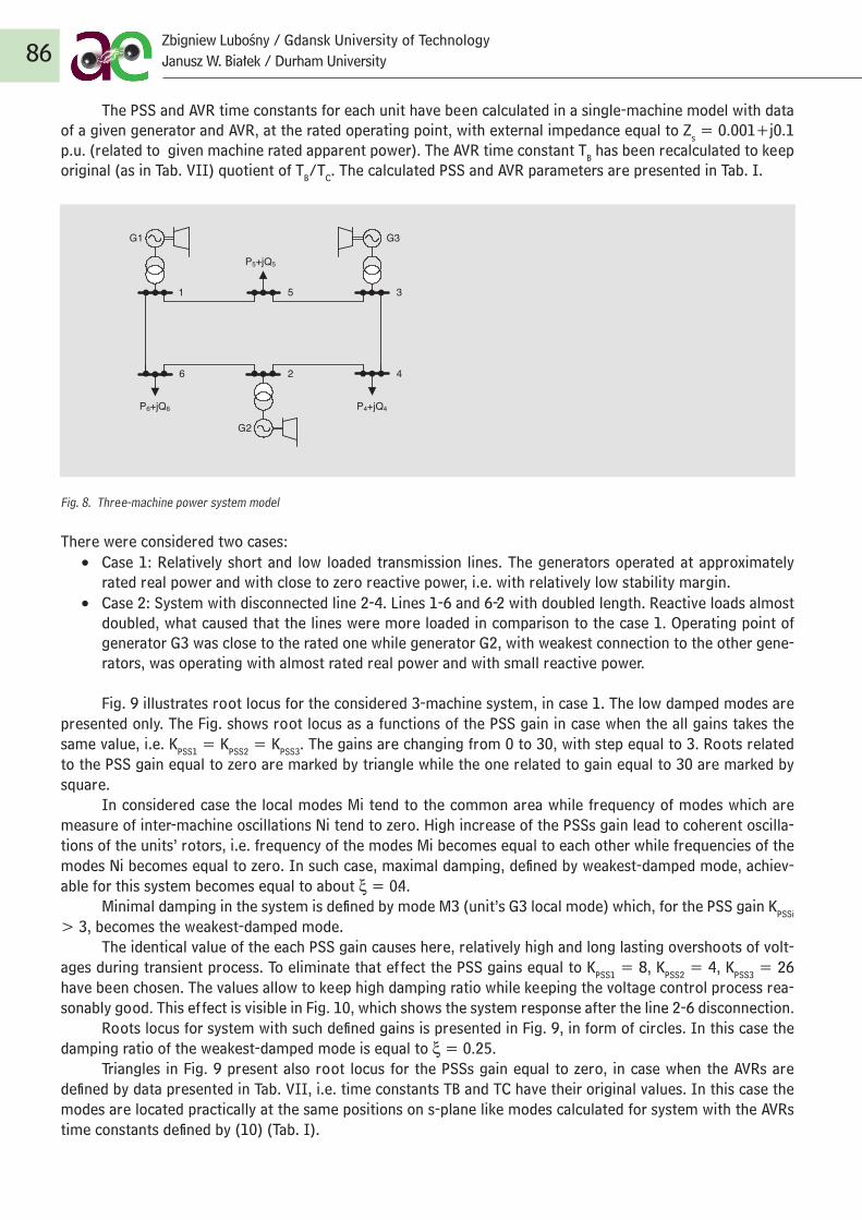
The PSS and AVR time constants for each unit have been calculated in a single-machine model with data of a given generator and AVR, at the rated operating point, with external impedance equal to Zs = 0.001+j0.1 p.u. (related to given machine rated apparent power). The AVR time constant TB has been recalculated to keep original (as in Tab. VII) quotient of TB/TC. The calculated PSS and AVR parameters are presented in Tab. I.
Fig. 8. Three-machine power system model
There were considered two cases:• Case 1: Relatively short and low loaded transmission lines. The generators operated at approximately
rated real power and with close to zero reactive power, i.e. with relatively low stability margin. • Case 2: System with disconnected line 2-4. Lines 1-6 and 6-2 with doubled length. Reactive loads almost
doubled, what caused that the lines were more loaded in comparison to the case 1. Operating point of generator G3 was close to the rated one while generator G2, with weakest connection to the other gene-rators, was operating with almost rated real power and with small reactive power.
Fig. 9 illustrates root locus for the considered 3-machine system, in case 1. The low damped modes are presented only. The Fig. shows root locus as a functions of the PSS gain in case when the all gains takes the same value, i.e. KPSS1 = KPSS2 = KPSS3. The gains are changing from 0 to 30, with step equal to 3. Roots related to the PSS gain equal to zero are marked by triangle while the one related to gain equal to 30 are marked by square.
In considered case the local modes Mi tend to the common area while frequency of modes which are measure of inter-machine oscillations Ni tend to zero. High increase of the PSSs gain lead to coherent oscilla-tions of the units’ rotors, i.e. frequency of the modes Mi becomes equal to each other while frequencies of the modes Ni becomes equal to zero. In such case, maximal damping, defined by weakest-damped mode, achiev-able for this system becomes equal to about ξ = 0.4.
Minimal damping in the system is defined by mode M3 (unit’s G3 local mode) which, for the PSS gain KPSSi > 3, becomes the weakest-damped mode.
The identical value of the each PSS gain causes here, relatively high and long lasting overshoots of volt-ages during transient process. To eliminate that effect the PSS gains equal to KPSS1 = 8, KPSS2 = 4, KPSS3 = 26 have been chosen. The values allow to keep high damping ratio while keeping the voltage control process rea-sonably good. This effect is visible in Fig. 10, which shows the system response after the line 2-6 disconnection.
Roots locus for system with such defined gains is presented in Fig. 9, in form of circles. In this case the damping ratio of the weakest-damped mode is equal to ξ = 0.25.
Triangles in Fig. 9 present also root locus for the PSSs gain equal to zero, in case when the AVRs are defined by data presented in Tab. VII, i.e. time constants TB and TC have their original values. In this case the modes are located practically at the same positions on s-plane like modes calculated for system with the AVRs time constants defined by (10) (Tab. I).
86Zbigniew Lubośny / Gdansk University of TechnologyJanusz W. Białek / Durham University
13
1
G1
426
5 3
G3
G2
P5+jQ5
P6+jQ6 P4+jQ4
Rys. 8. Struktura systemu trzymaszynowego
RozwaŜano dwa warianty pracy systemu:
• Wariant 1: Względnie krótkie i dość słabo obciąŜone linie elektroenergetyczne. Punkty pracy
generatorów synchronicznych bliskie granicy stabilności lokalnej, ze znamionową generacją mocy
czynnej
• Wariant 2: System z wyłączoną linią 2–4. Linie 1–6 i 6–2 o zdwojonej, w stosunku do wariantu 1,
długości. ObciąŜenia mocą bierną w węzłach odbiorczych równieŜ zdwojone. Punkt pracy generatora
G3 zbliŜony do znamionowego. Generator G2, najsłabiej związany z resztą systemu
elektroenergetycznego, obciąŜony praktycznie znamionową mocą czynną i małą mocą bierną.
Rys. 9 przedstawia rozmieszczenie biegunów układu trzymaszynowego (zlinearyzowanego) dla wariantu 1,
przy czym prezentowane są tu tylko wartości własne najsłabiej tłumionych modów. Pokazano tu zaleŜność
połoŜenia biegunów od współczynnika wzmocnienia stabilizatorów systemowych, gdy wartości tych
współczynników dla wszystkich trzech stabilizatorów są sobie równe, tj. KPSS1 = KPSS2 = KPSS3. Wartości
tych współczynników zmieniają się w przedziale od 0 do 30, z krokiem równym 3. Wartości własne dla
współczynnika wzmocnienia stabilizatorów systemowych równego 0 (zero) oznaczone są trójkątami, a dla
równego 30-kwadratami.
W prezentowanym przypadku, w miarę wzrostu wartości współczynnika wzmocnienia stabilizatora
systemowego, mody kołysań lokalnych Mi zmierzają do wspólnego obszaru, natomiast częstotliwości
modów będących miarą kołysań międzyobszarowych (międzygeneratorowych) Ni zmierzają do zera.
Wzrost współczynników wzmocnienia stabilizatorów systemowych powoduje, Ŝe kołysania wirników
generatorów stają się koherentne, tzn. częstotliwości modów kołysań lokalnych Mi stają się sobie równe, a
częstotliwości kołysań między obszarowych (międzygeneratorowych) Ni dąŜą do zera. W tym przypadku
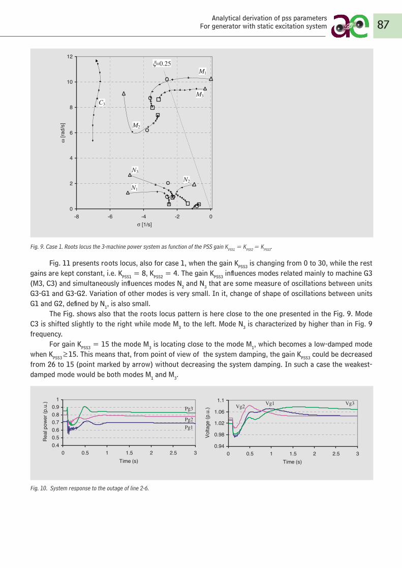
Fig. 9. Case 1. Roots locus the 3-machine power system as function of the PSS gain KPSS1 = KPSS2 = KPSS3.
Fig. 11 presents roots locus, also for case 1, when the gain KPSS3 is changing from 0 to 30, while the rest gains are kept constant, i.e. KPSS1 = 8, KPSS2 = 4. The gain KPSS3 influences modes related mainly to machine G3 (M3, C3) and simultaneously influences modes N2 and N3 that are some measure of oscillations between units G3-G1 and G3-G2. Variation of other modes is very small. In it, change of shape of oscillations between units G1 and G2, defined by N1, is also small.
The Fig. shows also that the roots locus pattern is here close to the one presented in the Fig. 9. Mode C3 is shifted slightly to the right while mode M3 to the left. Mode N3 is characterized by higher than in Fig. 9 frequency.
For gain KPSS3 = 15 the mode M3 is locating close to the mode M1, which becomes a low-damped mode when KPSS3 ≥ 15. This means that, from point of view of the system damping, the gain KPSS3 could be decreased from 26 to 15 (point marked by arrow) without decreasing the system damping. In such a case the weakest-damped mode would be both modes M1 and M3.
Fig. 10. System response to the outage of line 2-6.
87Analytical derivation of pss parameters
For generator with static excitation system
14
maksymalne tłumienie kołysań elektromechanicznych, definiowane przez współczynnik tłumienia modu
najsłabiej tłumionego, jest równe ξ = 0,4.
Minimalne tłumienie w systemie określa mod M3 (mod kołysań lokalnych generatora G3), który dla KPSSi >
3 staje się modem najsłabiej tłumionym.
Przyjęcie jednakowych wartości współczynnika wzmocnienia wszystkich stabilizatorów systemowych
powoduje tu występowanie względnie duŜych i długo trwających przeregulowań napięcia generatorów w
odpowiedzi na zaburzenie stanu pracy układu. W celu wyeliminowania tego efektu przyjęto wartości
współczynników wzmocnienia równe KPSS1 = 8, KPSS2 = 4, KPSS3 = 26. Wartości te pozwalają utrzymać
dobre tłumienie kołysań elektromechanicznych, zapewniając równocześnie dobre odpowiedzi napięciowe
generatorów. Uzyskany w tym przypadku efekt przedstawiono na rys. 10, pokazującym odpowiedź układu
na wyłączenie linii 2–6.
Rozmieszczenie biegunów na rys. 9 przedstawiają kółka, współczynnik tłumienia najsłabiej tłumionego
modu elektromechanicznego jest równy ξ = 0,25.
Trójkąty na rys. 9 przedstawiają równieŜ połoŜenie biegunów układu dla zerowych wartości
współczynnika wzmocnienia i równocześnie dla parametrów regulatorów napięcia równych wartościom
tzw. oryginalnym, przedstawionym w tab. VII, tj. z rzeczywistymi (z obiektów rzeczywistych) wartościami
stałych czasowych TB i TC. W tym przypadku lokalizacja wartości własnych jest praktycznie identyczna jak
lokalizacja wartości własnych dla obliczenia regulatorów napięcia z wartościami parametrów obliczonymi
na podstawie zaleŜności (10) (tab. I).
0
2
4
6
8
10
12
-8 -6 -4 -2 0σ [1/s]
ω [r
ad/s
]
N1
N2
N3
M2
M1
M3
C3
ξ=0.25
6
transient process. To eliminate that effect the PSS gains equal to KPSS1 = 8, KPSS2 = 4, KPSS3 = 26 have been chosen. The values allow to keep high damping ratio while keeping the voltage control process reasonably good. This effect is visible in Fig. 10, which shows the system response after the line 2-6 disconnection.
Roots locus for system with such defined gains is presented in Fig. 9, in form of circles. In this case the damping ratio of the weakest-damped mode is equal to ξ = 0.25.
Triangles in Fig. 9 present also root locus for the PSSs gain equal to zero, in case when the AVRs are defined by data presented in Tab. VII, i.e. time constants TB and TC have their original values. In this case the modes are located practically at the same positions on s-plane like modes calculated for system with the AVRs time constants defined by (10) (Tab. I).
0
2
4
6
8
10
12
-8 -6 -4 -2 0σ [1/s]
ω [r
ad/s
]
Fig. 9. Case 1. Roots locus the 3-machine power system as function of the PSS gain KPSS1 = KPSS2 = KPSS3.
Fig. 11 presents roots locus, also for case 1, when the gain KPSS3 is changing from 0 to 30, while the rest gains are kept constant, i.e. KPSS1 = 8, KPSS2 = 4. The gain KPSS3 influences modes related mainly to machine G3 (M3, C3) and simultaneously influences modes N2 and N3 that are some measure of oscillations between units G3-G1 and G3-G2. Variation of other modes is very small. In it, change of shape of oscillations between units G1 and G2, defined by N1, is also small.
The Fig. shows also that the roots locus pattern is here close to the one presented in the Fig. 9. Mode C3 is shifted slightly to the right while mode M3 to the left. Mode N3 is characterized by higher than in Fig. 9 frequency.
For gain KPSS3 = 15 the mode M3 is locating close to the mode M1, which becomes a low-damped mode when KPSS3 ≥15. This means that, from point of view of the system damping, the gain KPSS3 could be decreased from 26 to 15 (point marked by arrow) without decreasing the system
damping. In such a case the weakest-damped mode would be both modes M1 and M3.
0.40.50.60.70.80.9
1
0 0.5 1 1.5 2 2.5 3Time (s)
Real
pow
er (p
.u.)
0.94
0.98
1.02
1.06
1.1
0 0.5 1 1.5 2 2.5 3Time (s)
Volta
ge (p
.u.)
Fig. 10. System response to the outage of line 2-6.
0
2
4
6
8
10
12
-8 -6 -4 -2 0σ [1/s]
ω [r
ad/s
]
Fig. 11. Case 1. Roots locus in the 3-machine power system as function of the PSS gain KPSS3.
Finally, Fig. 12 illustrates roots locus for the 3-machine system, in case 2. As previously, the all PSSs gain is equal to each other and changes from 0 to 30. Like in the previous case the circles show root locus for system with various gains (KPSS1= 8, KPSS2= 4, KPSS3= 26).
Maximum damping, achievable for this system, for KPSSi >> 30, is also equal to about ξ = 0.4. For the PSSs with various gains the damping ratio of the weakest-damped mode is equal to ξ = 0.24, which is practically the same value like in the case 1.
The minimal damping in the system is defined by mode M1, until the PSS gain KPSSi will reach 21. Next, the damping ratio
Pg1Pg2
Pg3
Vg2 Vg1 Vg3
N1
N2
N3
M2
M1
M3
C3
ξ=0.25
M3
M1
M2
C3
N2
N3
N1
KPSS3 =15
6
transient process. To eliminate that effect the PSS gains equal to KPSS1 = 8, KPSS2 = 4, KPSS3 = 26 have been chosen. The values allow to keep high damping ratio while keeping the voltage control process reasonably good. This effect is visible in Fig. 10, which shows the system response after the line 2-6 disconnection.
Roots locus for system with such defined gains is presented in Fig. 9, in form of circles. In this case the damping ratio of the weakest-damped mode is equal to ξ = 0.25.
Triangles in Fig. 9 present also root locus for the PSSs gain equal to zero, in case when the AVRs are defined by data presented in Tab. VII, i.e. time constants TB and TC have their original values. In this case the modes are located practically at the same positions on s-plane like modes calculated for system with the AVRs time constants defined by (10) (Tab. I).
0
2
4
6
8
10
12
-8 -6 -4 -2 0σ [1/s]
ω [r
ad/s
]
Fig. 9. Case 1. Roots locus the 3-machine power system as function of the PSS gain KPSS1 = KPSS2 = KPSS3.
Fig. 11 presents roots locus, also for case 1, when the gain KPSS3 is changing from 0 to 30, while the rest gains are kept constant, i.e. KPSS1 = 8, KPSS2 = 4. The gain KPSS3 influences modes related mainly to machine G3 (M3, C3) and simultaneously influences modes N2 and N3 that are some measure of oscillations between units G3-G1 and G3-G2. Variation of other modes is very small. In it, change of shape of oscillations between units G1 and G2, defined by N1, is also small.
The Fig. shows also that the roots locus pattern is here close to the one presented in the Fig. 9. Mode C3 is shifted slightly to the right while mode M3 to the left. Mode N3 is characterized by higher than in Fig. 9 frequency.
For gain KPSS3 = 15 the mode M3 is locating close to the mode M1, which becomes a low-damped mode when KPSS3 ≥15. This means that, from point of view of the system damping, the gain KPSS3 could be decreased from 26 to 15 (point marked by arrow) without decreasing the system
damping. In such a case the weakest-damped mode would be both modes M1 and M3.
0.40.50.60.70.80.9
1
0 0.5 1 1.5 2 2.5 3Time (s)
Real
pow
er (p
.u.)
0.94
0.98
1.02
1.06
1.1
0 0.5 1 1.5 2 2.5 3Time (s)
Volta
ge (p
.u.)
Fig. 10. System response to the outage of line 2-6.
0
2
4
6
8
10
12
-8 -6 -4 -2 0σ [1/s]
ω [r
ad/s
]
Fig. 11. Case 1. Roots locus in the 3-machine power system as function of the PSS gain KPSS3.
Finally, Fig. 12 illustrates roots locus for the 3-machine system, in case 2. As previously, the all PSSs gain is equal to each other and changes from 0 to 30. Like in the previous case the circles show root locus for system with various gains (KPSS1= 8, KPSS2= 4, KPSS3= 26).
Maximum damping, achievable for this system, for KPSSi >> 30, is also equal to about ξ = 0.4. For the PSSs with various gains the damping ratio of the weakest-damped mode is equal to ξ = 0.24, which is practically the same value like in the case 1.
The minimal damping in the system is defined by mode M1, until the PSS gain KPSSi will reach 21. Next, the damping ratio
Pg1Pg2
Pg3
Vg2 Vg1 Vg3
N1
N2
N3
M2
M1
M3
C3
ξ=0.25
M3
M1
M2
C3
N2
N3
N1
KPSS3 =15
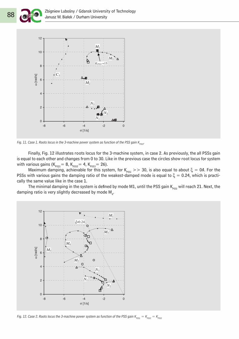
Fig. 11. Case 1. Roots locus in the 3-machine power system as function of the PSS gain KPSS3.
Finally, Fig. 12 illustrates roots locus for the 3-machine system, in case 2. As previously, the all PSSs gain is equal to each other and changes from 0 to 30. Like in the previous case the circles show root locus for system with various gains (KPSS1= 8, KPSS2= 4, KPSS3= 26).
Maximum damping, achievable for this system, for KPSSi >> 30, is also equal to about ξ = 0.4. For the PSSs with various gains the damping ratio of the weakest-damped mode is equal to ξ = 0.24, which is practi-cally the same value like in the case 1.
The minimal damping in the system is defined by mode M1, until the PSS gain KPSSi will reach 21. Next, the damping ratio is very slightly decreased by mode M4.
Fig. 12. Case 2. Roots locus the 3-machine power system as function of the PSS gain KPSS1 = KPSS2 = KPSS3
88Zbigniew Lubośny / Gdansk University of TechnologyJanusz W. Białek / Durham University
16
0
2
4
6
8
10
12
-8 -6 -4 -2 0σ [1/s]
ω [r
ad/s
]
Rys. 11. Wariant 1. Lokalizacja biegunów układu trzymaszynowego w funkcji współczynnika
wzmocnienia stabilizatora systemowego KPSS3
Na zakończenie, rys. 12 przedstawia połoŜenie modów systemu dla wariantu 2. Jak poprzednio,
współczynniki wzmocnienia stabilizatorów systemowych, równe sobie, zmieniają się od 0 do 30. RównieŜ
jak poprzednio, kółka pokazują połoŜenia biegunów układu dla systemu z róŜnymi współczynnikami
wzmocnienia stabilizatorów systemowych, równych odpowiednio KPSS1 = 8, KPSS2 = 4, KPSS3 = 26.
Maksymalne tłumienie kołysań w tym systemie, osiągane dla KPSSi >> 30, jest równieŜ równe około ξ =
0,4. W przypadku systemu z róŜnymi współczynnikami wzmocnienia współczynnik tłumienia najsłabiej
tłumionego modu jest równy ξ = 0,24, co jest wartością porównywalną z uzyskaną poprzednio (w
wariancie 1).
Minimalne tłumienie w układzie określa mod M1 do chwili, gdy współczynnik wzmocnienia KPSSi osiąga
wartość 21. Dalej współczynnik tłumienia jest słabo ograniczany przez mod M4.
M3
M1
M2
C3
N2
N3
N1
KPSS3 =15
17
0
2
4
6
8
10
12
-8 -6 -4 -2 0σ [1/s]
ω [r
ad/s
]
Rys. 12. Wariant 2. Lokalizacja biegunów układu trzymaszynowego w funkcji współczynników
wzmocnienia stabilizatorów systemowych dla przypadku KPSS1 = KPSS2 = KPSS3
VI. WNIOSKI
W artykule przedstawiono sposób analitycznego określania parametrów stabilizatora systemowego
quasi-idealnego, tj. takiego, który wytwarza tylko moment tłumiący w szerokim przedziale zmian
częstotliwości kołysań elektromechanicznych. Metoda oparta jest na modelu generatora synchronicznego 3.
rzędu i zastosowana dla generatora ze statycznym układem wzbudzenia i regulacji napięcia oraz
stabilizatora systemowego z prędkością kątową wirnika jako sygnałem wejściowym. Metoda jest czuła na
strukturę regulatora napięcia, zatem zaleŜności pozwalające określać nastawy stabilizatora systemowego
zaleŜą od przyjętej struktury regulatora. W artykule przedstawiono zaleŜności dla jednej struktury
regulatora napięcia i jej dwóch podstruktur.
Wartości parametrów stabilizatora zaleŜą od danych obiektu (generatora), danych regulatora napięcia,
punktu pracy generatora oraz impedancji zewnętrznej. PoniewaŜ dwie ostatnie wielkości są zmienne w
trakcie pracy systemu, optymalny stabilizator systemowy powinien charakteryzować się zmiennymi
wartościami parametrów. W praktyce stosuje się jednak stabilizatory (a takŜe regulator napięcia)
stacjonarne. Przeprowadzone testy wykazały, Ŝe równieŜ proponowany stabilizator systemowy jest
efektywny w wariancie stacjonarnym.
PoniewaŜ parametry stabilizatora systemowego związane są z parametrami regulatora napięcia, wartości
niektórych parametrów regulatora napięcia powinny być określane równocześnie z wartościami
N2
N3
N1
M1
M2
M5
M3
M4
ξ=0.24

VI. CONCLUSIONSThe paper presents way of deriving equations that allow to calculate parameters of PSS that produces
a damping torque only in a wide frequency range. The derivation is based on the 3rd order single-machine infinite-busbar model and is applied here for generator with static exciter and speed-based PSS. Because the method is the AVR structure sensitive, as result, three sets of equations allowing to calculate PSS parameters for three various structures of AVR are presented.
The PSS parameters defined by proposed equations depend on plant data, AVR parameters, system op-erating point and external impedance. Because of the latter two, the PSS parameters should vary during plant operation but tests have proved that the proposed PSS in form of a time-invariant controller performs almost equally well.
The PSS parameters are related to some of the AVR parameters and therefore should be set simultane-ously.
Advantage of the proposed methodology is simplicity of the PSS design. PSS time constants can be cal-culated directly, using a single-machine steady-state model, without any iterative optimization process. Simula-tions have shown that the values derived in a single-machine system (by applying the proposed equations) are valid also in a multi-machine system.
The proposed method has been verified for large units operating in transmission system and for smaller units operating in distribution systems (results not presented here) giving in the all cases good results. The method seems to be especially suited for units operating in the distribution systems because the distribution systems operates as radial and the transmission system, from point of view of such units, can be treated as in-finite busbar. Then solution achieved for the single-machine system directly match to generating unit operating in the distribution system.
Low amount and accessibility of data that is necessary to calculate the PSS (and AVR) parameters allow us to implement the derived equations in any digital controller of synchronous generator. In such a case the PSS parameters and some AVR parameters can be calculated just by the synchronous generator controller.
The equations proposed in the paper allow us to define PSS that effectiveness is similar to effectiveness of the well tuned PSS, which parameters are defined by using GEP or P-Vr methodology. This is because the all mentioned methods are based on damping torque concept and, especially because they utilize the same struc-ture of PSS, which in fact defines limits of such PSS efficiency.
VIII. APPENDIX
A. Linear model of single-machine infinite busbar system
X’d = Xl+Xad− Xad×Xad/Xf
RT = Rl+Rt+Rs, XTq = Xq+Xt+Xs, XTd = X’d+Xt+Xs
D = RT×RT+XTd×XTq
m1 = Vs(XTq×sinδ−RT
×cosδ)/D, n1 = Vs (RT×sinδ+XTd
×cosδ)/D
m2 = XTq×Xad/(D×Xf), n2 = RT
×Xad/(D×Xf)
K1 = Eq×n1+Iq
×(Xq-X’d)m1
K2 = Xad[RT×Eq/D+(1+XTq
×(Xq− X’d)/D)Iq]/Xf
K3 = Xf/[Xadu×(1+(Xd−X’d)×XTq/D)], K4 = Xadu
×Xad×m1/Xf
K5 = (-Rl×m1+Xq
×n1) sinδ+(−Rl×n1-X’d×m1)cosδ
K6 = (−Rl×m2+Xq
×n2)sinδ+[−Rl×n2-X’d×m2+(X’d−Xl)/(Xf-Xad)]cosδ
T3 = Xf/[ω0×Rf(1+XTq(Xd−X’d)/D)]
89Analytical derivation of pss parameters
For generator with static excitation system
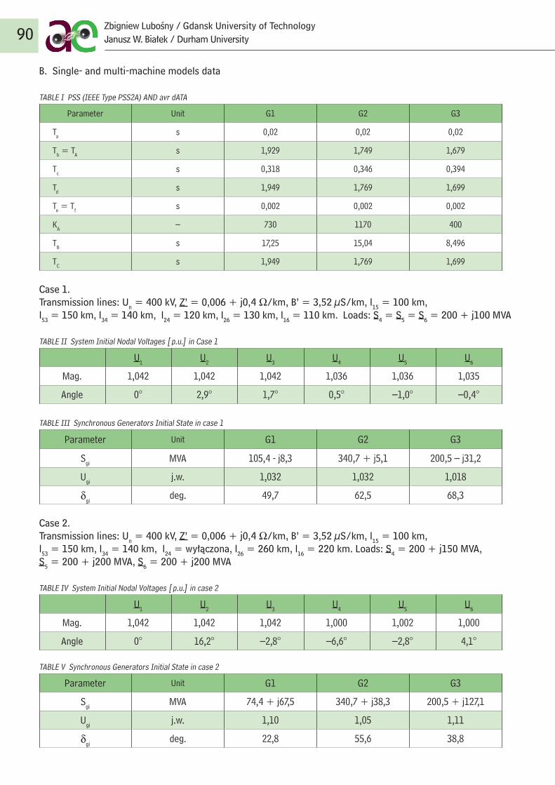
B. Single- and multi-machine models data
TABLE I PSS (IEEE Type PSS2A) AND avr dATA
Parameter Unit G1 G2 G3
Ta s 0,02 0,02 0,02
Tb = TA s 1,929 1,749 1,679
Tc s 0,318 0,346 0,394
Td s 1,949 1,769 1,699
Te = Tf s 0,002 0,002 0,002
KA – 730 1170 400
TB s 17,25 15,04 8, 496
TC s 1,949 1,769 1,699
Case 1.Transmission lines: Un = 400 kV, Z’ = 0,006 + j0, 4 Ω/km, B’ = 3,52 µS/km, l15 = 100 km, l53 = 150 km, l34 = 140 km, l24 = 120 km, l26 = 130 km, l16 = 110 km. Loads: S4 = S5 = S6 = 200 + j100 MVA
TABLE II System Initial Nodal Voltages [p.u.] in Case 1
U1 U2 U3 U4 U5 U6
Mag. 1,042 1,042 1,042 1,036 1,036 1,035
Angle 0° 2,9° 1,7° 0,5° –1,0° –0, 4°
TABLE III Synchronous Generators Initial State in case 1
Parameter Unit G1 G2 G3
Sgi MVA 105, 4 - j8,3 340,7 + j5,1 200,5 – j31,2
Ugi j.w. 1,032 1,032 1,018
δgideg. 49,7 62,5 68,3
Case 2. Transmission lines: Un = 400 kV, Z’ = 0,006 + j0, 4 Ω/km, B’ = 3,52 µS/km, l15 = 100 km, l53 = 150 km, l34 = 140 km, l24 = wyłączona, l26 = 260 km, l16 = 220 km. Loads: S4 = 200 + j150 MVA, S5 = 200 + j200 MVA, S6 = 200 + j200 MVA
TABLE IV System Initial Nodal Voltages [p.u.] in case 2
U1 U2 U3 U4 U5 U6
Mag. 1,042 1,042 1,042 1,000 1,002 1,000
Angle 0° 16,2° –2,8° –6,6° –2,8° 4,1°
TABLE V Synchronous Generators Initial State in case 2
Parameter Unit G1 G2 G3
Sgi MVA 74, 4 + j67,5 340,7 + j38,3 200,5 + j127,1
Ugi j.w. 1,10 1,05 1,11
δgideg. 22,8 55,6 38,8
90Zbigniew Lubośny / Gdansk University of TechnologyJanusz W. Białek / Durham University
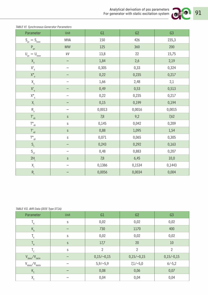
TABLE VI Synchronous Generator Parameters
Parameter Unit G1 G2 G3
Sgn = Sbase MVA 150 426 235,3
Pgn MW 125 360 200
Ugn = Ubase kV 13,8 22 15,75
Xd – 1,84 2,6 2,19
X’d – 0,305 0,33 0,324
X”d – 0,22 0,235 0,217
Xq – 1,66 2, 48 2,1
X’q – 0, 49 0,53 0,513
X”q – 0,22 0,235 0,217
Xl – 0,15 0,199 0,194
R a – 0,0013 0,0016 0,0015
T’d0 s 7,8 9,2 7,62
T”d0 s 0,145 0,042 0,209
T’q0 s 0,88 1,095 1,54
T”q0 s 0,071 0,065 0,305
S1 – 0,243 0,292 0,163
S12 – 0, 48 0,883 0,207
2Hj s 7,8 6, 45 10,0
Xt – 0,1386 0,1534 0,1443
Rt – 0,0056 0,0034 0,004
TABLE VII. AVR Data (IEEE Type ST1A)
Parameter Unit G1 G2 G3
TR s 0,02 0,02 0,02
KA – 730 1170 400
TA s 0,02 0,02 0,02
TB s 17,7 20 10
TC s 2 2 2
VIMAX/VIMIN – 0,15/–0,15 0,15/–0,15 0,15/-0,15
VRMAX/VRMIN – 5,9/–5,9 7,1/–5,0 6/-5,2
KC – 0,08 0,06 0,07
XC – 0,04 0,04 0,04
91Analytical derivation of pss parameters
For generator with static excitation system
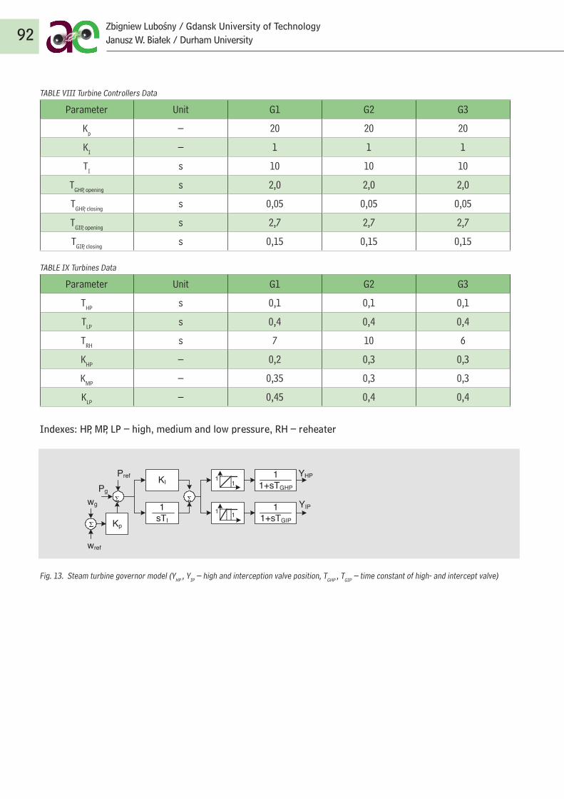
TABLE VIII Turbine Controllers Data
Parameter Unit G1 G2 G3
Kp – 20 20 20
KI – 1 1 1
TI s 10 10 10
TGHP, opening s 2,0 2,0 2,0
TGHP, closing s 0,05 0,05 0,05
TGIP, opening s 2,7 2,7 2,7
TGIP, closing s 0,15 0,15 0,15
TABLE IX Turbines Data
Parameter Unit G1 G2 G3
THP s 0,1 0,1 0,1
TLP s 0, 4 0, 4 0, 4
TRH s 7 10 6
KHP – 0,2 0,3 0,3
KMP – 0,35 0,3 0,3
KLP – 0, 45 0, 4 0, 4
Indexes: HP, MP, LP – high, medium and low pressure, RH – reheater
Fig. 13. Steam turbine governor model (YHP , YIP – high and interception valve position, TGHP , TGIP – time constant of high- and intercept valve)
92Zbigniew Lubośny / Gdansk University of TechnologyJanusz W. Białek / Durham University
22
miary
THP s 0,1 0,1 0,1
TLP s 0,4 0,4 0,4
TRH s 7 10 6
KHP – 0,2 0,3 0,3
KMP – 0,35 0,3 0,3
KLP – 0,45 0,4 0,4
Indeksy: HP, MP, LP – wysoko-, średnio- i niskopręŜny, RH – przegrzewacz międzystopniowy.
KI
1sTI
11
11 1
1+sTGHP
YHP
YIP
Pref
wref
Pg
Kp
wg 11+sTGIP
Rys. 13. Model regulatora turbiny (YHP, YIP – połoŜenie zaworów wysokopręŜnych i intercepcyjnych
turbiny, TGHP, TGIP – stałe czasowe zaworów wysokopręŜnych i intercepcyjnych)
Bibliografia
1. IEEE Std 421.5-1992: IEE Recommended Practice for Excitation System Models for Power System
Stability Studies, IEEE, New York 1992, ISBN 1–55937–218–4.
2. Mello de F.P., Concordia C., Concepts of Synchronous Machine Stability as Affected by Excitation
Control, IEEE Trans. Power Appar. Syst., vol. 88, 1969, s. 316–329.
3. Larsen E.V., Swann D.A., Applying Power System Stabilizer, IEEE Trans. Power Appar. Syst., vol. 100,
1981, s. 3017–3046.
4. Mello de F.P., Czuba J.S., Rushe P.A., Willis J.R., Developments in Application of Stabilising Measures
Through Excitation Control, Paper Ref. 38-05, CIGRE Session 1986.
5. Gibbard M.J., Co-ordinated design of multimachine power system stabilizers based on damping torque
concept, Proc. Inst. Elect. Eng. C, vol. 135, no. 4, July 1988, s. 276–284.
6. Gibbard M.J., Robust Design of Fixed-parameter Power System Stabilisers over a Wide Range of
Operating Conditions, IEEE Trans. Power Syst., vol. 6, no. 2, May 1991, s. 794–800.
7. Gibbard M. J., Vowles D. J., Reconciliation of Methods of Compensation for PSSs in Multimachine
System, IEEE Trans. Power Syst., vol. 19, no. 1, February 2004, s. 463–472.
8. Kundur P., Power system stability and control, New York: McGraw–Hill, 1994, s. 761.
Σ Σ
Σ

LITERATURE
1. IEEE Std 421.5-1992: IEE Recommended Practice for Excitation System Models for Power System Stability Studies, IEEE, New York 1992, ISBN 1–55937–218–4.
2. Mello de F.P., Concordia C., Concepts of Synchronous Machine Stability as Affected by Excitation Control, IEEE Trans. Power Appar. Syst., vol. 88, 1969, s. 316–329.
3. Larsen E.V., Swann D.A., Applying Power System Stabilizer, IEEE Trans. Power Appar. Syst., vol. 100, 1981, s. 3017–3046.4. Mello de F.P., Czuba J.S., Rushe P.A., Willis J.R., Developments in Application of Stabilising Measures Through Exci-
tation Control, Paper Ref. 38-05, CIGRE Session 1986.5. Gibbard M.J., Co-ordinated design of multimachine power system stabilizers based on damping torque concept,
Proc. Inst. Elect. Eng. C, vol. 135, no. 4, July 1988, s. 276–284.6. Gibbard M.J., Robust Design of Fixed-parameter Power System Stabilisers over a Wide Range of Operating Condi-
tions, IEEE Trans. Power Syst., vol. 6, no. 2, May 1991, s. 794–800.7. Gibbard M.J., Vowles D.J., Reconciliation of Methods of Compensation for PSSs in Multimachine System, IEEE Trans.
Power Syst., vol. 19, no. 1, February 2004, s. 463–472.8. Kundur P., Power system stability and control, New York: McGraw–Hill, 1994, s. 761.9. Machowski J., Bialek J., Bumby J.R., Power System Dynamics and Stability, New York: John Wiley and Sons, 1997, s. 291.10. CIGRE Task Force 38.02.16, Impact of Interactions among Power Systems, Paris, August 2000.11. CIGRE Task Force 38.01.07, Analysis and Control of Power System Oscillations, Paris, December 1996.12. Lee D.C., Kundur P., Advanced Excitation Controls for Power System Stability Enhancement, Paper Ref., no 38–01,
CIGRE Session 1986.13. Murdoch Dr.A., Venkataraman S., Lawson R.A., Pearson W.R., Integral of Accelerating Power Type PSS. Part 1 –
Theory, Design, and Tuning Methodology. Part 2 – Field Testing and Performance Verification, IEEE Trans. on Energy Conv., vol. 14, no. 4, December 1999, s. 1658–1672.
93Analytical derivation of pss parameters
For generator with static excitation system

94 Ryszard Michniewski / ENERGA-OPERATOR S.A. Toruń Branch
Ryszard MichniewskiToruń / Polska
Ryszard Michniewski obtained his diploma at the Electrical Engineering Faculty at the Poznań University of Technology. He began his profes-sional career as a constructor in Pomorskie Zakłady Wytwórcze Aparatury Niskiego Napięcia in Toruń. Later he worked as production mainte-nance engineer in Pomorskie Zakłady Przemysłu Wapiennego Bielawy. Since 1962, he has worked at various positions at Zakłady Energetyczne in Toruń, till his retirement in 2004. Today, he is involved in training and implementation of live working technique (PPN technology) projects on overhead high and extra high voltage lines in ENERGA-OPERATOR SA He is a member of Polskie Towarzystwo Przesyłu i Rozdziału Energii Elektrycznej [Polish As-sociation of Electrical Power Transmission and Distribution], member of Polski Komitet Bezpieczeństwa w Energetyce [Polish Energy Security Committee] and Association of Polish Electrical Engineers (SEP).
Author / Biographie

PPN - live conductor operations on 400 kv, 220 kv and 110 kv overhead transmission and distribution lines in ENERGA-OPERATOR S.A., Toruń Branch 95
PPN - LIVE CONDUCTOR OPERATIONS ON 400 KV, 220 KV AND 110 KV OVERHEAD TRANSMISSION AND DISTRIBUTION LINES IN ENERGA-OPERATOR S.A.TORUŃ BRANCH
Ryszard Michniewski / ENERGA-OPERATOR S.A. Toruń Branch
The history of live-working techniques (PPN) on high and extra high voltage overhead lines in ENERGA-OPERATOR S.A. Toruń Branch dates back to 1933 when the first operations applying the PPN technology took place in Pomorska Elektrownia Krajowa Gródek (previously ENERGA-OPERATOR S.A., Toruń Branch ) on the 60 kV line Gródek – Gdynia. Revival of PPN operations on overhead transmission lines took place in 1990 on 400 kV lines using equipment and technologies purchased in the former German Democratic Republic.
1992 marked the beginning of performing PPN operations on straight line poles and straight and trans-position line poles for 220 kV based on technologies developed in Zakład Energetyczny in Toruń in cooperation with the Occupational Work Safety Section at the Institute of Power Engineering in Gliwice In 2008, ENERGA-OPERATOR S.A., Toruń Branch developed and implemented a technology for replacing insulators and insulator assemblies on anchor poles and anchor and angle poles.
The paper presents the short history of hotline operations (PPN) on 400 kV, 220 kV overhead transmis-sion lines and 110 kV lines from the first PPN operations performed by ENERGA-OPERATOR S.A. Toruń Branch to the end of 2008. The volume of work performed on the lines is shown and the kinds of operations. The paper describes the methodology and technologies applied du-ring the operations. Pictures are included showing ope-rations on 400 kV, 220 kV, 110 kV and the design of the derrick for transporting the fitter to the 400 kV hotlines and the insulator string to the pole lines. The operations
applying PPN technology performed on 400 kV, 220 kV and 110 kV lines provided grounds for conclusions regar-ding the reduction of line power loss, i.e. the positive eco-nomic and environmental impact of the PPN technology.
Abstract
YearLine
Total400 kV 220 kV
1990 2 - 21991 5 - 51992 7 2 91993 2 35 371994 2 94 961995 6 20 261996 5 16 211997 26 1 271998 4 3 71999 1 2 32000 1 9 102001 8 1 92002 1 3 42003 1 9 102004 174 2 1762005 199 1 2002006 194 20 2142007 128 34 1622008 103 32 135
Razem 869 284 1153
Table 2 shows operations in particular years.
Table 1 shows the number of PPN technology operations on 400kV and 220kV lines in the period 1990 to the end of 2008.
Number of operations on lines:
Total number of operations
400 kV 220 kV
Poles Poles
Anchor and angle
polesStraight
line polesStraight and transposition
poles
Anchor and angle
poles
245 624 260 24 1153
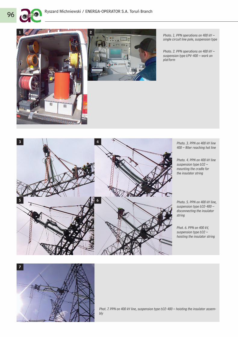
96
Photo. 1. PPN operations on 400 kV – single circuit line pole, suspension type
Photo. 2. PPN operations on 400 kV – suspension type ŁPV-400 – work on platform
Phot. 7. PPN on 400 kV line, suspension type ŁO2-400 – hoisting the insulator assem-bly
Photo. 3. PPN on 400 kV line 400 – fitter reaching hot line
Photo. 4. PPN on 400 kV line suspension type ŁO2 – mounting the cradle for the insulator string
Photo. 5. PPN on 400 kV line, suspension type ŁO2-400 – disconnecting the insulator string
Phot. 6. PPN on 400 kV, suspension type ŁO2 – hoisting the insulator string
Ryszard Michniewski / ENERGA-OPERATOR S.A. Toruń Branch
3
1
5
4
2
6
7
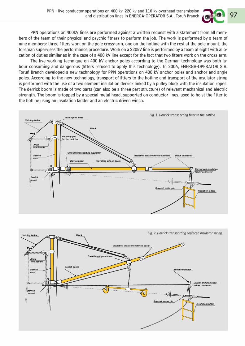
PPN operations on 400kV lines are performed against a written request with a statement from all mem-bers of the team of their physical and psychic fitness to perform the job. The work is performed by a team of nine members: three fitters work on the pole cross-arm, one on the hotline with the rest at the pole mount, the foreman supervises the performance procedure. Work on a 220kV line is performed by a team of eight with allo-cation of duties similar as in the case of a 400 kV line except for the fact that two fitters work on the cross-arm.
The live working technique on 400 kV anchor poles according to the German technology was both la-bour consuming and dangerous (fitters refused to apply this technology). In 2006, ENERGA-OPERATOR S.A. Toruń Branch developed a new technology for PPN operations on 400 kV anchor poles and anchor and angle poles. According to the new technology, transport of fitters to the hotline and transport of the insulator string is performed with the use of a two element insulation derrick linked by a pulley block with the insulation ropes. The derrick boom is made of two parts (can also be a three part structure) of relevant mechanical and electric strength. The boom is topped by a special metal head, supported on conductor lines, used to hoist the fitter to the hotline using an insulation ladder and an electric driven winch.
97PPN - live conductor operations on 400 kv, 220 kv and 110 kv overhead transmission
and distribution lines in ENERGA-OPERATOR S.A., Toruń Branch
Head top on mast
Hoisting tackle
Block
Mounting grip
for top rack bar
Angle
iron handle
Grip with transporting supporter
Derrick Insulation stick connecter on boom Boom connector
mast
Derrick boom
Derrick and insulation
ladder connector
Derrick
mount
Support, cotter pin
Insulation ladder
Travelling grip on boom
Fig. 1. Derrick transporting fitter to the hotline
Hoisting tackle Block
Angle iron handle
Insulation stick connecter on boom
Travelling grip on boom
Derrick boomDerrick Boom connectormast
Derrick and insulationladder connector
derrick mount
Support, cotter pin Insulation ladder
Fig. 2. Derrick transporting replaced insulator string

An application to the Patent Office of the Republic of Poland was submitted in 2007 for PPN operations on anchor poles and anchor and angle poles to obtain patent protection for the new technology. It is entered under the number P 382278.
In 2008, ENERGA-OPERATOR SA Toruń Branch developed and implemented the new technology for the live working technique on 220 kV anchor poles and anchor and angle pole lines, suspension type ŁO2 and ŁO3. Development of the technology was quite difficult because most 220 kV lines base on VKLF 75/16 and VKLS 75/21 type long rod insulators, which have a high damage rate. For this reason conductors and insulator strings cannot be used in hoisting the fitter to the hot line and for fitter’s operations on the hotline from the conductor side. To enable the replacement of insulator and insulation assemblies, suspension type ŁO2 and ŁO3, (long rod insulation), the control of tension line must be ensured prior to the operation. Special holders/clamps have been constructed (made of steel, aluminium or plastic) placed on the strain yoke of insulator string on the side of the conductor and on the side of the pole structure. Thanks to these clamps for insulation sticks and pull, the line strain functions are reallocated and allow for the replacement of insulators and assemblies. The fitter is transported to the hotline with use of an insulated ladder, which is hoisted with an insulation system com-prising a six meter long and ø 75 mm insulation stick, metal cable head, insulation rollers and angle clamps. The insulation system is fastened in two points to the lower angle bar of the pole cross-arm. Operations on the insulator string from the conductor side are performed by the operator on the insulated ladder, connected to the insulation assembly. The insulation head is supported during the operation by the insulation derrick boom (for better bracing). An application for patenting this technology is being at present processed by the Polish Patent Office.
98 Ryszard Michniewski / ENERGA-OPERATOR S.A. Toruń Branch
Fig. 3. Derrick – selecting boom length relevant for the line bend angle
Block
Boom connector
Derrick boom
Derrick and insulationladder connector
Support, cotter pin
Insulation ladder
Segment part 1 – diameter 110 Segment part 3
3.1.
Insulation stick connecter on boom
800
4800
3.2.
Travelling grip on boom
Segment part 2 – diameter 110
2500
Segment part 3 – dimension in (mm)
3.5.3.4.3.3.
500800900
11001200
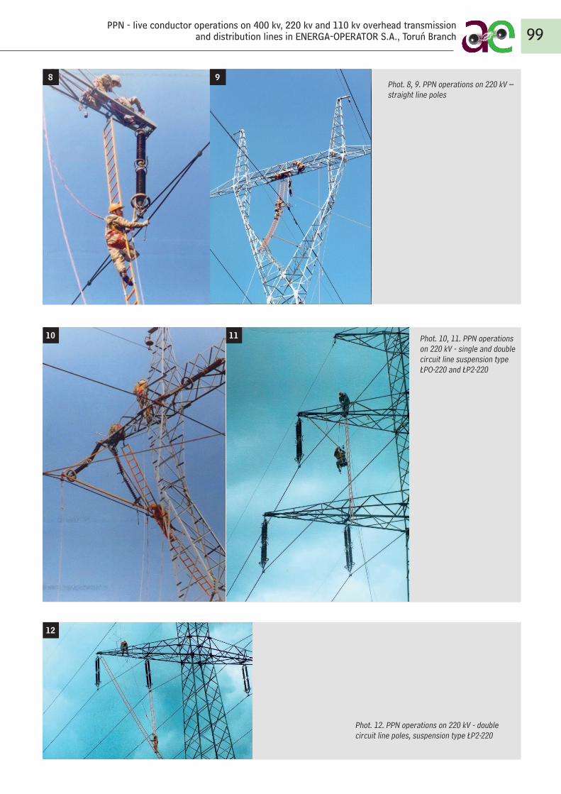
99
Phot. 8, 9. PPN operations on 220 kV – straight line poles
Phot. 12. PPN operations on 220 kV - double circuit line poles, suspension type ŁP2-220
Phot. 10, 11. PPN operations on 220 kV - single and double circuit line suspension type ŁPO-220 and ŁP2-220
PPN - live conductor operations on 400 kv, 220 kv and 110 kv overhead transmission and distribution lines in ENERGA-OPERATOR S.A., Toruń Branch
10
8
11
9
12

Table 3 presents the scope of works on 400kV and 220kV lines applying PPN technology.
No. Year Line Scope of operations
1 1993–1995 220 kV line Włocławek Azoty – Pątnów Replacement of 318 VKLF 75/16 on straight line poles and straight line and transposition poles
2 2004 Double circuit 400kV line Gdańsk Błonia – Żarnowiec Replacement of 141 slings on straight line poles
3 2005 400 kV line Grudziądz Węgrowo – Płock Replacement of 74 PS16B insulators on straight line poles and repair of 73 surge arrester bridges
4 2005 400 kV line Krajnik – Dunowo Replacement of 74 PS16B insulators on 57 straight line poles
5 2006 400 kV line Dunowo – Słupsk Replacement of 100 PS16A insulators on straight line poles and 9 PS22A on anchor poles
6 2006 400 kV line Słupsk – Żarnowiec Replacement of 38 PS22A insulators in 35 rows, suspension type ŁO2 and ŁO3
7 2006 220 kV line Dunowo – Żydowo Replacement of 21 PS16B insulators on straight line poles
8 2006 400 kV line Krajnik – Dunowo Replacement of 8 PS22A insulators, suspension type ŁO2 and ŁO3, and replacement of 28 insulators PS16B, suspension type ŁP and ŁPV
9 2007 400 kV line Połaniec – Rzeszów Replacement of 20 insulators, suspension type ŁO2 and ŁO3
10 2007 400 kV line Krajnik – Dunowo Replacement of 121 PS22A insulators, suspension type ŁO2 and ŁO3 and 24 PS16B insulators, suspension type ŁP and ŁPV
11 2007 220 kV line Olsztyn – Ostrołęka Replacement of 114 insulators LP 75/17 assembly, suspension type ŁPO on straight line and transposition poles
12 2008 400 kV line Krajnik – DunowoReplacement of 26 insulators PS16B, suspension types ŁP and ŁPV on straight line poles and replacement of 86 insulators PS22A, suspension type ŁO2 and ŁO3 on anchor lines, in total 110 pieces in 103 rows
13 2008 220 kV line Olsztyn – Ostrołęka Replacement of 30 insulators LP 75/17 assembly, suspension type ŁPO, and 48 assemblies suspension type ŁO2
The first PPN operations on overhead transmission lines took place in 1998 on 110 kV lines. Up to date, the only company applying PPN technology for this voltage is ENERGA-OPERATOR SA, Toruń Branch .
Operations on overhead 110 kV transmission lines apply two methods.• remote method• hotline method – developed by ENERGA-OPERATOR SA, Toruń Branch in 2007.
Remote operations on 110 kV straight lines with use of insulations sticks with heads, which hold the ap-propriate tools (their dimensions cannot exceed 300x300x150 mm), and a pulley block with insulation ropes. PPN operations on anchor and angle poles are performed with the help of; a two part insulation derrick mounted on the pole shaft, insulation pull with hooks placed on the conductor, and by the anchor clamp and insulation sticks holding relevant tools.
PPN operations on 110 kV straight lines are performed by a team of six. Two fitters work on the pole structure, four on the pole mount, the foreman supervises the performance procedure. PPN operations on an-chor poles are performed by a team of seven. Three fitters work on the pole structure, four on the pole mount. The work is performed at a written request for the service supplemented by a statement of the team members confirming their physical and psychic fitness to perform the operation applying PPN technology.
Table 4 shows the number of operations performed by ENERGA-OPERATOR SA, Toruń Branch on 110 kV lines.
Table 4.
Year Number of PPN operations
Number of operations on poles Number of replaced insulators
Average time required for insulator replacement on poles
Straight poles Straight and transition poles
Anchor and angle poles Straight poles Anchor and
angle poles1998 68 51 17 - 98 50 min -1999 361 346 15 - 403 53 min -2000 294 250 44 - 447 1 h 12 min -2001 22 19 3 - 25 60 min -2002 250 231 19 - 275 50 min -2003 87 1 - 86 104 1 h 15 min 1 h 50 min2004 353 208 - 145 479 44 min 1 h 17 min2005 835 295 19 521 1401 50 min 1 h2006 931 477 45 409 1291 48 min 59 min2007 836 349 3 484 1358 48 min 58 min2008 740 210 12 518 1331 46 min 60 min
Razem 4777 2437 177 2163 7212
100 Ryszard Michniewski / ENERGA-OPERATOR S.A. Toruń Branch
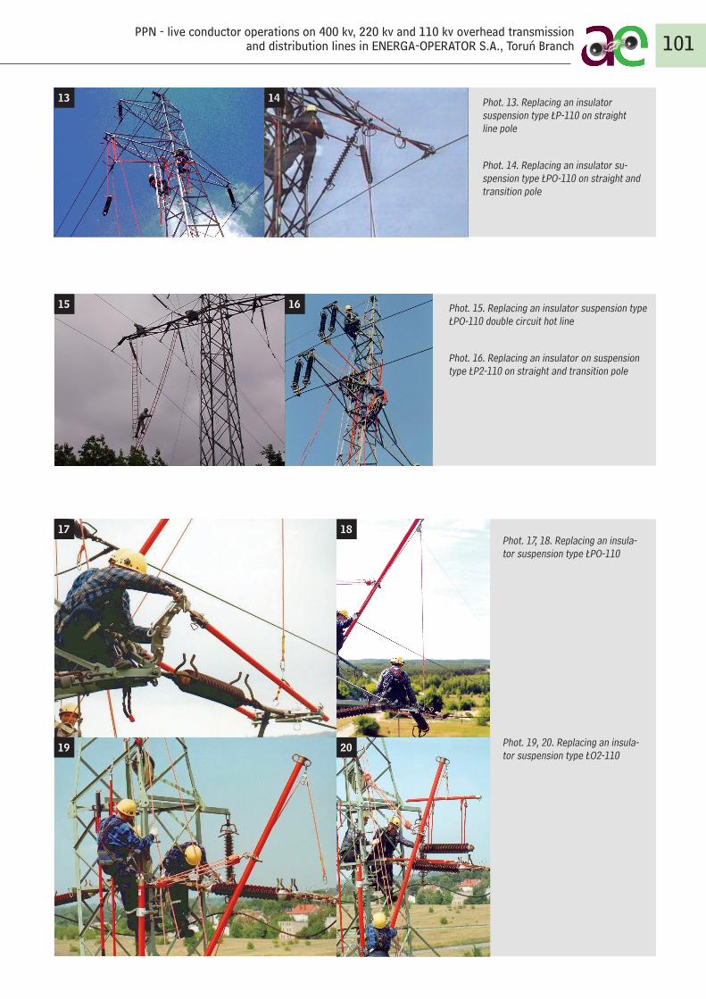
101
Phot. 13. Replacing an insulator suspension type ŁP-110 on straight line pole
Phot. 14. Replacing an insulator su-spension type ŁPO-110 on straight and transition pole
Phot. 17, 18. Replacing an insula-tor suspension type ŁPO-110
Phot. 19, 20. Replacing an insula-tor suspension type ŁO2-110
Phot. 15. Replacing an insulator suspension type ŁPO-110 double circuit hot line
Phot. 16. Replacing an insulator on suspension type ŁP2-110 on straight and transition pole
PPN - live conductor operations on 400 kv, 220 kv and 110 kv overhead transmission and distribution lines in ENERGA-OPERATOR S.A., Toruń Branch
15
13
17 18
2019
16
14
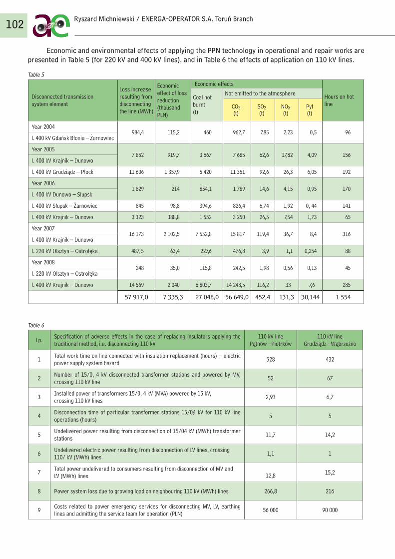
Economic and environmental effects of applying the PPN technology in operational and repair works are presented in Table 5 (for 220 kV and 400 kV lines), and in Table 6 the effects of application on 110 kV lines.
Table 5
Disconnected transmission system element
Loss increase resulting from disconnecting the line (MWh)
Economic effect of loss reduction(thousand PLN)
Economic effects
Hours on hot line
Coal not burnt(t)
Not emitted to the atmosphere
CO2(t)
SO2(t)
NOx(t)
Pył(t)
Year 2004 984, 4 115,2 460 962,7 7,85 2,23 0,5 96
l. 400 kV Gdańsk Błonia – Żarnowiec
Year 2005 7 852 919,7 3 667 7 685 62,6 17,82 4,09 156
l. 400 kV Krajnik – Dunowo
l. 400 kV Grudziądz – Płock 11 606 1 357,9 5 420 11 351 92,6 26,3 6,05 192
Year 2006 1 829 214 854,1 1 789 14,6 4,15 0,95 170
l. 400 kV Dunowo – Słupsk
l. 400 kV Słupsk – Żarnowiec 845 98,8 394,6 826, 4 6,74 1,92 0, 44 141
l. 400 kV Krajnik – Dunowo 3 323 388,8 1 552 3 250 26,5 7,54 1,73 65
Year 200716 173 2 102,5 7 552,8 15 817 119, 4 36,7 8, 4 316
l. 400 kV Krajnik – Dunowo
l. 220 kV Olsztyn – Ostrołęka 487, 5 63, 4 227,6 476,8 3,9 1,1 0,254 88
Year 2008 248 35,0 115,8 242,5 1,98 0,56 0,13 45
l. 220 kV Olsztyn – Ostrołęka
l. 400 kV Krajnik – Dunowo 14 569 2 040 6 803,7 14 248,5 116,2 33 7,6 285
57 917,0 7 335,3 27 048,0 56 649,0 452,4 131,3 30,144 1 554
Table 6
Lp.Specification of adverse effects in the case of replacing insulators applying the traditional method, i.e. disconnecting 110 kV
110 kV line Pątnów –Piotrków
110 kV line Grudziądz –Wąbrzeźno
1Total work time on line connected with insulation replacement (hours) – electric power supply system hazard
528 432
2Number of 15/0, 4 kV disconnected transformer stations and powered by MV, crossing 110 kV line
52 67
3Installed power of transformers 15/0, 4 kV (MVA) powered by 15 kV, crossing 110 kV lines
2,93 6,7
4Disconnection time of particular transformer stations 15/0,4 kV for 110 kV line operations (hours)
5 5
5Undelivered power resulting from disconnection of 15/0,4 kV (MWh) transformer stations
11,7 14,2
6Undelivered electric power resulting from disconnection of LV lines, crossing 110/ kV (MWh) lines
1,1 1
7Total power undelivered to consumers resulting from disconnection of MV and LV (MWh) lines 12,8 15,2
8 Power system loss due to growing load on neighbouring 110 kV (MWh) lines 266,8 216
9Costs related to power emergency services for disconnecting MV, LV, earthing lines and admitting the service team for operation (PLN)
56 000 90 000
102 Ryszard Michniewski / ENERGA-OPERATOR S.A. Toruń Branch

PPN operations on 400 kV, 220 kV and 110 kV overhead transmission lines mean:• operation of electric power supply systems without hazard,• reduction of power loss in the transmission and distribution system,• no disconnecting of crossing 220 kV, 110 kV, MV and LV lines,• no restrictions in electric power sales from extra high voltage, HV, MV and LV systems, • reduction of power system operational costs,• improving Occupational Safety and Hygiene in operational and repair jobs,• developing proper habits in operational and repair jobs,• increasing the operational level,• reduction of time required for the operation,• more environmental friendly way.
BIBLIOGRAFIA
1. Michniewski R., Aspekty techniczne i ekonomiczne prowadzenia prac pod napięciem w ZE Toruń SA, Energetyka, 2002, nr 10/11.
2. Michniewski R., Czy warto wykonywać PPN na liniach przesyłowych w Polsce?, Energetyka, 2006, nr 6 i Biuletyn Informacyjny PTPiREE, 2006, nr 4.
3. Michniewski R., Prace pod napięciem na słupach odporowych i odporowo-narożnych linii 400 kV – uzyskiwane efekty ekonomiczne, IX Konferencja „Prace pod napięciem w sieciach nn, SN i WN w Polsce i na świecie”, Gdańsk 21–22.06.2007.
4. Michniewski R., Prace pod napięciem na słupach odporowych i odporowo-narożnych linii 400kV – efekty ekonomicz-ne, Biuletyn Branżowy, 2007, nr 8, Energia elektryczna, PTPiREE.
5. Krawulski A., Niejadlik T., Prace pod napięciem na liniach 400 kV i 220 kV wykonywane w Koncernie ENERGA SA Oddział w Toruniu, VIII Międzynarodowa Konferencja ICOLIM 2006, Czechy, Praga, 7–9.06.2006.
6. Michniewski R., Prace pod napięciem realizowane przez ENERGA-OPERATOR SA Oddział w Toruniu na sieci prze-syłowej 400 kV, 220 kV i 110 kV – uzyskane efekty ekonomiczne i związane z ochroną środowiska, IX Międzynarodowa Konferencja ICOLIM 2008 Polska, Toruń, 4–6.06.2008.
7. Dmoch K., Konieczny Z., Prace pod napięciem w ENERGA-OPERATOR SA – nowe technologie na liniach napowietrz-nych WN, IX Międzynarodowa Konferencja ICOLIM 2008 Polska, Toruń, 4–6.06.2008.
8. Michniewski R., Michniewski D., Niejadlik T., Wykonywanie prac pod napięciem w Polsce na napowietrznych liniach 110 kV, VII Międzynarodowa Konferencja ICOLIM 2004, Rumunia, Bukareszt, 25–27.05.2004.
103PPN - live conductor operations on 400 kv, 220 kv and 110 kv overhead transmission
and distribution lines in ENERGA-OPERATOR S.A., Toruń Branch

104Sławomir Noske / ENERGA-OPERATOR S.A. Elbląg Branch
Sławomir NoskeElbląg / Polska
Head of the ENERGA-OPERATOR S.A. Elbląg Branch Techni-cal Department in the Elbląg Electricity Distribution Region. Employed by the company since 1991. Graduate of the Poznań University of Technology Faculty of Electrical Engineering. Also completed postgraduate law and management studies at the Gdansk University of Technol-ogy as well as MBA studies at the Gdansk Foundation for Management Development. In 2006 began writing doctoral thesis on: ‘Diagnosis of medium voltage power lines using the self-extinguishing voltage wave method of measuring partial discharges.’ (Diagnostyka linii kablowych średniego napięcia z wykorzystaniem badania wyładowań niezupełnych metodą samogasnącej fali napięciowej.)
Since 1995 has been working in a team for implementing a computer system to support the operation of electricity networks, and is currently in charge of the implementation and further development of this system. Since 2004 is in charge of work concerning the diagnosis of MV cables on the basis of partial discharge measurements – using the Seba OWTS-25 system – and is a participant of a Poznań University of Technology Faculty of Electrical Engineering research project.
Author / Biographie
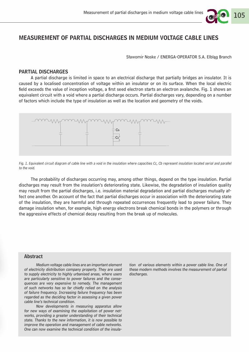
Measurement of partial discharges in medium voltage cable lines 105
MEASUREMENT OF PARTIAL DISCHARGES IN MEDIUM VOLTAGE CABLE LINES
Sławomir Noske / ENERGA-OPERATOR S.A. Elbląg Branch
PARTIAL DISCHARGES A partial discharge is limited in space to an electrical discharge that partially bridges an insulator. It is
caused by a localised concentration of voltage within an insulator or on its surface. When the local electric field exceeds the value of inception voltage, a first seed electron starts an electron avalanche. Fig. 1 shows an equivalent circuit with a void where a partial discharge occurs. Partial discharges vary, depending on a number of factors which include the type of insulation as well as the location and geometry of the voids.
Cb
Cc
Fig. 1. Equivalent circuit diagram of cable line with a void in the insulation where capacities Cc, Cb represent insulation located serial and parallel to the void.
The probability of discharges occurring may, among other things, depend on the type insulation. Partial discharges may result from the insulation’s deteriorating state. Likewise, the degradation of insulation quality may result from the partial discharges, i.e. insulation material degradation and partial discharges mutually af-fect one another. On account of the fact that partial discharges occur in association with the deteriorating state of the insulation, they are harmful and through repeated occurrences frequently lead to power failure. They damage insulation when, for example, high energy electrons break chemical bonds in the polymers or through the aggressive effects of chemical decay resulting from the break up of molecules.
Medium voltage cable lines are an important element of electricity distribution company property. They are used to supply electricity to highly urbanised areas, where users are particularly sensitive to power failures and the conse-quences are very expensive to remedy. The management of such networks has so far chiefly relied on the analysis of failure frequency. Increasing failure frequency has been regarded as the deciding factor in assessing a given power cable line’s technical condition.
Now developments in measuring apparatus allow for new ways of examining the exploitation of power net-works, providing a greater understanding of their technical state. Thanks to the new information, it is now possible to improve the operation and management of cable networks. One can now examine the technical condition of the insula-
tion of various elements within a power cable line. One of these modern methods involves the measurement of partial discharges.
Abstract

MEASUREMENT OF PARTIAL DISCHARGES Partial discharges were recognised as harmful to insulation already at the start of the 20th century, when
high voltage devices started being used. The first industrial tests of partial discharges were carried out in 1940. Developments in technology and computer science in the last decades of the 20th century allowed for the
construction of devices able to measure partial discharges in active power distribution networks.One of the solutions allowing for the measurement of partial discharges (PD) in medium voltage cables
is the Seba KMT OWTS-25 system. OWTS is currently used by the Elbląg branch of ENERGA-OPERATOR S.A.
Photo. 1. Cable test van using the OWTS-25 system
This system uses as the test voltage a self-extinguishing voltage wave. It is produced by raising the tested cable voltage to a required level and then discharging it through an air-core coil. The voltage frequency de-pends on the cable’s capacitance and the coil’s inductance. In tested cables this frequency is generally within the range of 200–800 Hz. Suppression of the voltage amplitude is associated with dielectric losses in the tested cable.
OWTS measures the voltage wave from the load induced during the partial discharge. It spreads in two opposite directions. The device first measures the wave heading for the cable end connected to it (the voltage wave proportional to the load value produced during the PD) and next the other wave after it has rebounded from the other end of the cable. Measurement of the time difference between the two waves allows us to locate exactly where the partial discharge occurred (Fig. 3). Pre-test calibration allows the device to measure PD load intensity in picoCoulombs (pC). This calibration is conducted in accordance with norm IEC 60270.
106Rozwój informatyczny i technologiczny w ostatnich dekadach XX wieku pozwolił na budowę
przewoźnych urządzeń dających możliwość pomiaru wyładowań niezupełnych w eksploatowanych
sieciach energetycznych.
Jednym z rozwiązań pozwalających mierzyć wyładowania niezupełne (wnz) w liniach kablowych
średniego napięcia jest system pomiarowy OWTS-25 firmy SEBA KMT. OWTS jest obecnie
wykorzystywany przez ENERGA-OPERATOR SA Oddział w Elblągu.
Rys. 2. Wóz pomiarowy z zainstalowanym systemem OWTS-25
System ten wykorzystuje jako napięcie probiercze samogasnacą falę napięciową. Wytwarzana
jest ona poprzez ładowanie badanego kabla do pożądanego napięcia, a następnie rozładowanie go
przez specjalnie zaprojektowaną cewkę bezrdzeniową. Częstotliwość napięcia zależna jest od
pojemności kabla i indukcyjności cewki. W praktyce, dla badanych linii kablowych mieści się
ona w granicach 200–800 Hz. Tłumienie zanikającej amplitudy napięcia związane jest ze
stratami dielektrycznymi w badanym kablu.
LCf
π2
1
OWTS mierzy falę napięciową powstałą od ładunku indukowanego podczas wyładowania
niezupełnego. Fala napięciowa rozchodzi się w dwóch kierunkach. Aparatura mierzy falę biegnącą w
kierunku końca z podłączoną aparaturą (fala napięciowa proporcjonalna do wartości ładunku
powstałego podczas wnz), a następnie falę odbitą od drugiego końca kabla. Pomiar różnicy czasu
między pomierzonymi falami pozwala określić miejsce wystąpienia wyładowania niezupełnego (rys.
3). Dokonana przed pomiarem kalibracja pozwala na wyskalowanie aparatury i pomiar
Sławomir Noske / ENERGA-OPERATOR S.A. Elbląg Branch
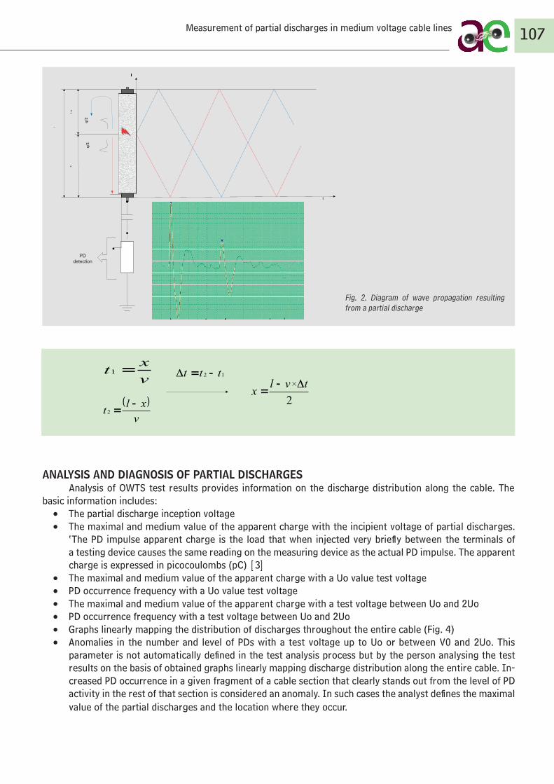
t
Detekcja wnz
lq
/2q
/2
l -x
x
l
ANALYSIS AND DIAGNOSIS OF PARTIAL DISCHARGES Analysis of OWTS test results provides information on the discharge distribution along the cable. The
basic information includes: • The partial discharge inception voltage • The maximal and medium value of the apparent charge with the incipient voltage of partial discharges.
‘The PD impulse apparent charge is the load that when injected very briefly between the terminals of a testing device causes the same reading on the measuring device as the actual PD impulse. The apparent charge is expressed in picocoulombs (pC) [3]
• The maximal and medium value of the apparent charge with a Uo value test voltage • PD occurrence frequency with a Uo value test voltage • The maximal and medium value of the apparent charge with a test voltage between Uo and 2Uo• PD occurrence frequency with a test voltage between Uo and 2Uo • Graphs linearly mapping the distribution of discharges throughout the entire cable (Fig. 4)• Anomalies in the number and level of PDs with a test voltage up to Uo or between V0 and 2Uo. This
parameter is not automatically defined in the test analysis process but by the person analysing the test results on the basis of obtained graphs linearly mapping discharge distribution along the entire cable. In-creased PD occurrence in a given fragment of a cable section that clearly stands out from the level of PD activity in the rest of that section is considered an anomaly. In such cases the analyst defines the maximal value of the partial discharges and the location where they occur.
107Measurement of partial discharges in medium voltage cable lines
intensywności wyładowania wnz w pikokulombach (pC). Kalibracja dokonywana jest zgodnie z PN-
EN 60270 (tłumaczenie międzynarodowej normy IEC 60270).
t
Detekcja
wnz
l
q/2
q/2
l -x
x
l
Rys. 3. Schematyczny obraz rozchodzenia się fali powstałej w wyniku wyładowania
niezupełnego
2
tvlx
Δ
v
xlt
2
12 ttt Δv
xt 1
Analiza i diagnoza wyładowań niezupełnych
Analiza wyników pomiaru dokonanych systemem OWTS dostarcza informacji o rozkładzie
wyładowań w funkcji długości kabla. Do podstawowych informacji uzyskanych z analizy
należą:
Napięcie początkowe wyładowań niezupełnych
Wartość średnia i maksymalna ładunku pozornego przy napięciu początkowym
wyładowań niezupełnych. „Ładunek pozorny impulsu wnz odpowiada ładunkowi,
który wstrzyknięty w bardzo krótkim czasie między zaciski obiektu badanego
Fig. 2. Diagram of wave propagation resulting from a partial discharge
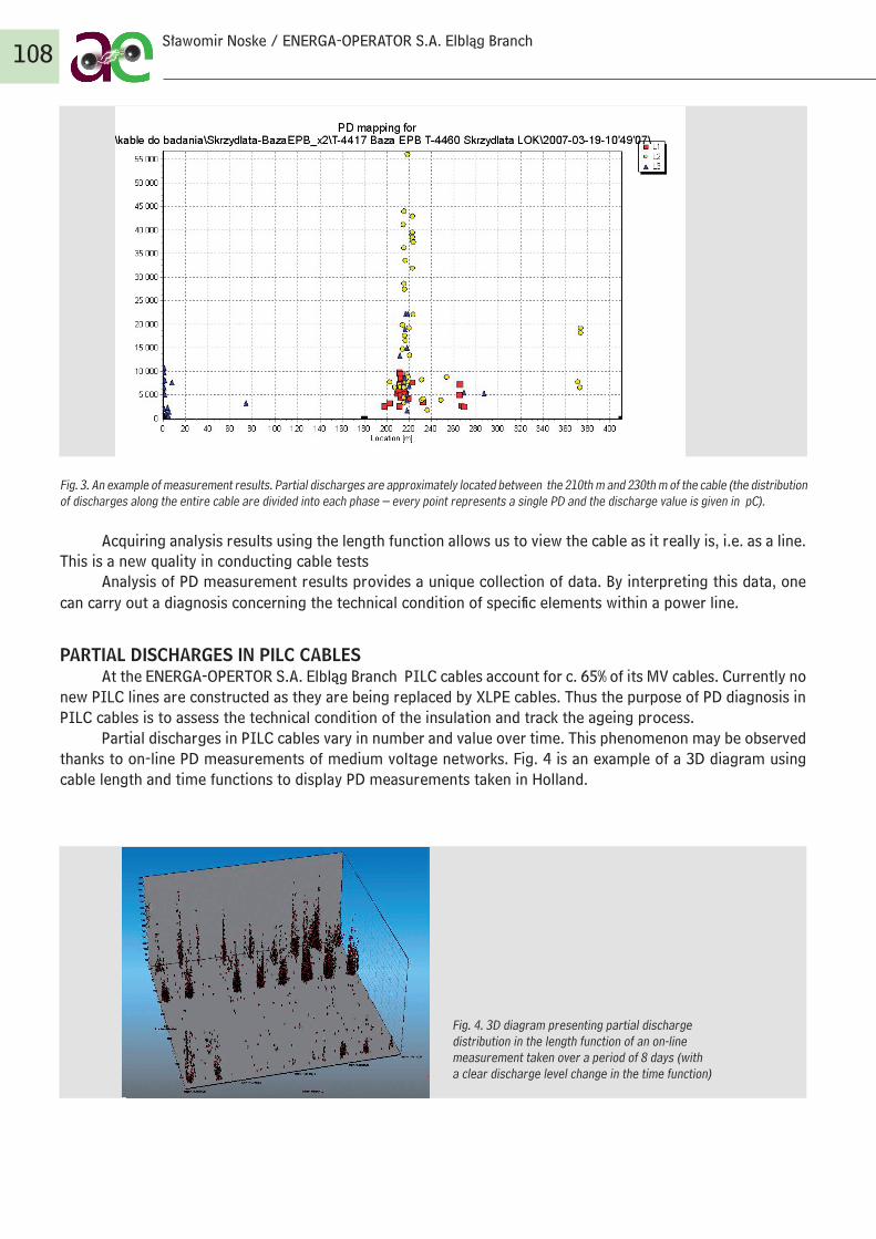
Fig. 3. An example of measurement results. Partial discharges are approximately located between the 210th m and 230th m of the cable (the distribution of discharges along the entire cable are divided into each phase – every point represents a single PD and the discharge value is given in pC).
Acquiring analysis results using the length function allows us to view the cable as it really is, i.e. as a line. This is a new quality in conducting cable tests
Analysis of PD measurement results provides a unique collection of data. By interpreting this data, one can carry out a diagnosis concerning the technical condition of specific elements within a power line.
PARTIAL DISCHARGES IN PILC CABLESAt the ENERGA-OPERTOR S.A. Elbląg Branch PILC cables account for c. 65% of its MV cables. Currently no
new PILC lines are constructed as they are being replaced by XLPE cables. Thus the purpose of PD diagnosis in PILC cables is to assess the technical condition of the insulation and track the ageing process.
Partial discharges in PILC cables vary in number and value over time. This phenomenon may be observed thanks to on-line PD measurements of medium voltage networks. Fig. 4 is an example of a 3D diagram using cable length and time functions to display PD measurements taken in Holland.
108
Fig. 4. 3D diagram presenting partial discharge distribution in the length function of an on-line measurement taken over a period of 8 days (with a clear discharge level change in the time function)
Sławomir Noske / ENERGA-OPERATOR S.A. Elbląg Branch
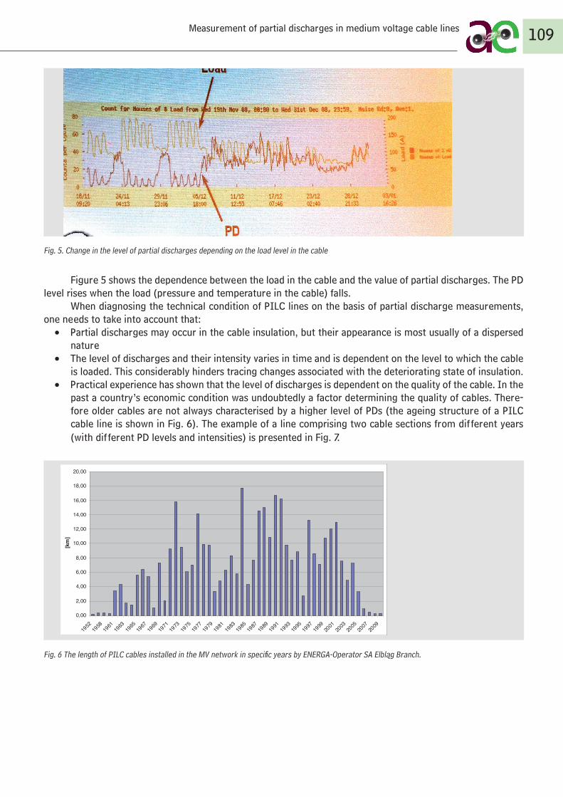
Fig. 5. Change in the level of partial discharges depending on the load level in the cable
Figure 5 shows the dependence between the load in the cable and the value of partial discharges. The PD level rises when the load (pressure and temperature in the cable) falls.
When diagnosing the technical condition of PILC lines on the basis of partial discharge measurements, one needs to take into account that:
• Partial discharges may occur in the cable insulation, but their appearance is most usually of a dispersed nature
• The level of discharges and their intensity varies in time and is dependent on the level to which the cable is loaded. This considerably hinders tracing changes associated with the deteriorating state of insulation.
• Practical experience has shown that the level of discharges is dependent on the quality of the cable. In the past a country’s economic condition was undoubtedly a factor determining the quality of cables. There-fore older cables are not always characterised by a higher level of PDs (the ageing structure of a PILC cable line is shown in Fig. 6). The example of a line comprising two cable sections from different years (with different PD levels and intensities) is presented in Fig. 7.
0,00
2,00
4,00
6,00
8,00
10,00
12,00
14,00
16,00
18,00
20,00
1952
1960
1963
1966
1969
1972
1975
1978
1981
1984
1987
1990
1993
1996
1999
2002
2005
2008
l [km
]
długość kabli PILC
Fig. 6 The length of PILC cables installed in the MV network in specific years by ENERGA-Operator SA Elbląg Branch.
109Measurement of partial discharges in medium voltage cable lines
0,00
2,00
4,00
6,00
8,00
10,00
12,00
14,00
16,00
18,00
20,00
1952
1958
1961
1963
1965
1967
1969
1971
1973
1975
1977
1979
1981
1983
1985
1987
1989
1991
1993
1995
1997
1999
2001
2003
2005
2007
2009
[km
]
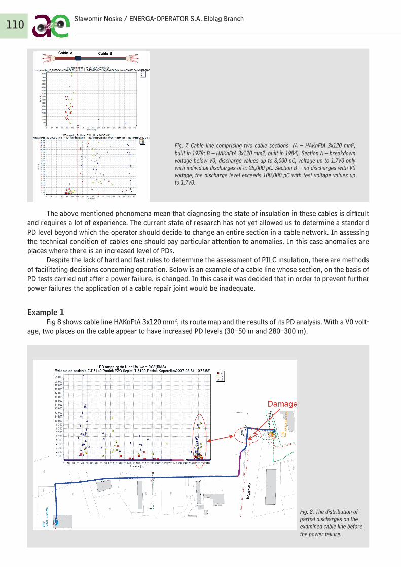
The above mentioned phenomena mean that diagnosing the state of insulation in these cables is difficult and requires a lot of experience. The current state of research has not yet allowed us to determine a standard PD level beyond which the operator should decide to change an entire section in a cable network. In assessing the technical condition of cables one should pay particular attention to anomalies. In this case anomalies are places where there is an increased level of PDs.
Despite the lack of hard and fast rules to determine the assessment of PILC insulation, there are methods of facilitating decisions concerning operation. Below is an example of a cable line whose section, on the basis of PD tests carried out after a power failure, is changed. In this case it was decided that in order to prevent further power failures the application of a cable repair joint would be inadequate.
Example 1Fig 8 shows cable line HAKnFtA 3x120 mm2, its route map and the results of its PD analysis. With a V0 volt-
age, two places on the cable appear to have increased PD levels (30–50 m and 280–300 m).
110Sławomir Noske / ENERGA-OPERATOR S.A. Elbląg Branch
Fig. 8. The distribution of partial discharges on the examined cable line before the power failure.
Fig. 7. Cable line comprising two cable sections (A – HAKnFtA 3x120 mm2, built in 1979; B – HAKnFtA 3x120 mm2, built in 1984). Section A – breakdown voltage below V0, discharge values up to 8,000 pC, voltage up to 1.7V0 only with individual discharges of c. 25,000 pC. Section B – no discharges with V0 voltage, the discharge level exceeds 100,000 pC with test voltage values up to 1.7V0.
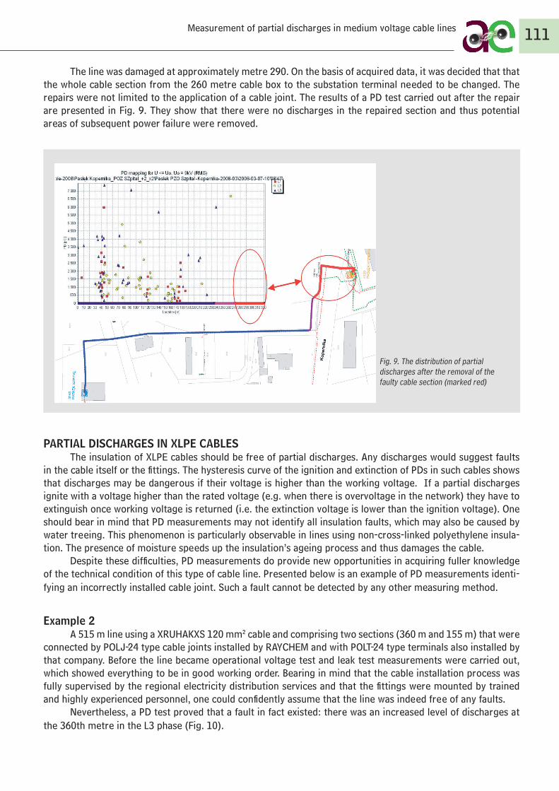
The line was damaged at approximately metre 290. On the basis of acquired data, it was decided that that the whole cable section from the 260 metre cable box to the substation terminal needed to be changed. The repairs were not limited to the application of a cable joint. The results of a PD test carried out after the repair are presented in Fig. 9. They show that there were no discharges in the repaired section and thus potential areas of subsequent power failure were removed.
PARTIAL DISCHARGES IN XLPE CABLESThe insulation of XLPE cables should be free of partial discharges. Any discharges would suggest faults
in the cable itself or the fittings. The hysteresis curve of the ignition and extinction of PDs in such cables shows that discharges may be dangerous if their voltage is higher than the working voltage. If a partial discharges ignite with a voltage higher than the rated voltage (e.g. when there is overvoltage in the network) they have to extinguish once working voltage is returned (i.e. the extinction voltage is lower than the ignition voltage). One should bear in mind that PD measurements may not identify all insulation faults, which may also be caused by water treeing. This phenomenon is particularly observable in lines using non-cross-linked polyethylene insula-tion. The presence of moisture speeds up the insulation’s ageing process and thus damages the cable.
Despite these difficulties, PD measurements do provide new opportunities in acquiring fuller knowledge of the technical condition of this type of cable line. Presented below is an example of PD measurements identi-fying an incorrectly installed cable joint. Such a fault cannot be detected by any other measuring method.
Example 2A 515 m line using a XRUHAKXS 120 mm2 cable and comprising two sections (360 m and 155 m) that were
connected by POLJ-24 type cable joints installed by RAYCHEM and with POLT-24 type terminals also installed by that company. Before the line became operational voltage test and leak test measurements were carried out, which showed everything to be in good working order. Bearing in mind that the cable installation process was fully supervised by the regional electricity distribution services and that the fittings were mounted by trained and highly experienced personnel, one could confidently assume that the line was indeed free of any faults.
Nevertheless, a PD test proved that a fault in fact existed: there was an increased level of discharges at the 360th metre in the L3 phase (Fig. 10).
111
Fig. 9. The distribution of partial discharges after the removal of the faulty cable section (marked red)
Measurement of partial discharges in medium voltage cable lines
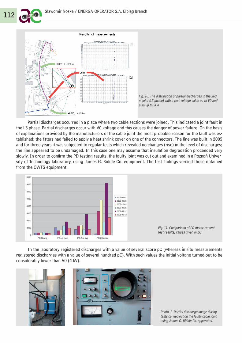
Partial discharges occurred in a place where two cable sections were joined. This indicated a joint fault in the L3 phase. Partial discharges occur with V0 voltage and this causes the danger of power failure. On the basis of explanations provided by the manufacturers of the cable joint the most probable reason for the fault was es-tablished: the fitters had failed to apply a heat shrink cover on one of the connectors. The line was built in 2005 and for three years it was subjected to regular tests which revealed no changes (rise) in the level of discharges; the line appeared to be undamaged. In this case one may assume that insulation degradation proceeded very slowly. In order to confirm the PD testing results, the faulty joint was cut out and examined in a Poznań Univer-sity of Technology laboratory, using James G. Biddle Co. equipment. The test findings verified those obtained from the OWTS equipment.
0
2000
4000
6000
8000
10000
12000
14000
16000
PD-Uośr PD-Uomax PD-2Uośr PD-2Uomax
2005-06-01
2005-09-26
2006-10-02
2007-01-25
2007-09-12
2008-02-12
In the laboratory registered discharges with a value of several score pC (whereas in situ measurements registered discharges with a value of several hundred pC). With such values the initial voltage turned out to be considerably lower than V0 (4 kV).
.
112
Fig. 11. Comparison of PD measurement test results, values given in pC
Photo. 2. Partial discharge image during tests carried out on the faulty cable joint using James G. Biddle Co. apparatus.
Sławomir Noske / ENERGA-OPERATOR S.A. Elbląg Branch
0
2000
4000
6000
8000
10000
12000
14000
16000
PD-Uo avg PD-Uo max PD-2Uo avg PD-2Uo max
2005-06-012005-09-262006-10-022007-01-252007-09-122008-02-12
Fig. 10. The distribution of partial discharges in the 360 m joint (L3 phase) with a test voltage value up to V0 and also up to 2Uo
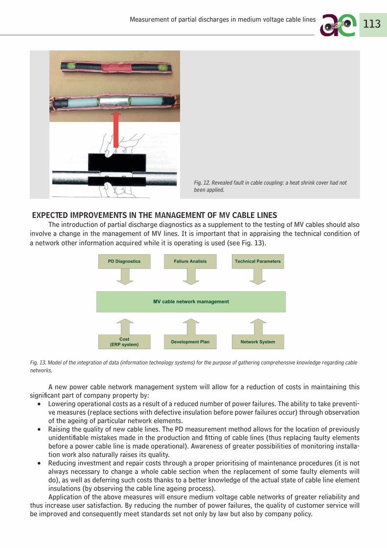
EXPECTED IMPROVEMENTS IN THE MANAGEMENT OF MV CABLE LINES The introduction of partial discharge diagnostics as a supplement to the testing of MV cables should also
involve a change in the management of MV lines. It is important that in appraising the technical condition of a network other information acquired while it is operating is used (see Fig. 13).
Fig. 13. Model of the integration of data (information technology systems) for the purpose of gathering comprehensive knowledge regarding cable networks.
A new power cable network management system will allow for a reduction of costs in maintaining this significant part of company property by:
• Lowering operational costs as a result of a reduced number of power failures. The ability to take preventi-ve measures (replace sections with defective insulation before power failures occur) through observation of the ageing of particular network elements.
• Raising the quality of new cable lines. The PD measurement method allows for the location of previously unidentifiable mistakes made in the production and fitting of cable lines (thus replacing faulty elements before a power cable line is made operational). Awareness of greater possibilities of monitoring installa-tion work also naturally raises its quality.
• Reducing investment and repair costs through a proper prioritising of maintenance procedures (it is not always necessary to change a whole cable section when the replacement of some faulty elements will do), as well as deferring such costs thanks to a better knowledge of the actual state of cable line element insulations (by observing the cable line ageing process). Application of the above measures will ensure medium voltage cable networks of greater reliability and
thus increase user satisfaction. By reducing the number of power failures, the quality of customer service will be improved and consequently meet standards set not only by law but also by company policy.
113
Fig. 12. Revealed fault in cable coupling: a heat shrink cover had not been applied.
Measurement of partial discharges in medium voltage cable lines
Cost (ERP system) Development Plan Network System
MV cable network mamagement
Faliure Analisis Technical ParametersPD Diagnostics

LITERATURE
1. Gulski E., Diagnozowanie wyładowań niezupełnych w urządzeniach wysokiego napięcia w eksploatacji, Warszawa, Oficyna Wydawnicza Politechniki Warszawskiej, 2003.
2. Guide for partial discharge measurements in compliance to IEC 60270, CIGRE Working Group D1.33, 2008.3. Noske S., Efektywne zarządzanie siecią kablową SN, Elektro-info, 2009, nr 1–2.4. Noske S., Wykorzystanie diagnostyki opartej o pomiar wyładowań niezupełnych do zarządzania siecią kablową
średniego napięcia, Konferencyjne Infotech 2008. 5. PN-EN 60270, Wysokonapięciowa technika probiercza. Pomiar wyładowań niezupełnych, PKN, Warszawa 2003.6. Rakowska A., Kryteria oceny weryfikujące jakość polietylenu usieciowanego stosowanego jako izolacja kabli elek-
troenergetycznych, Poznań, Wydawnictwo Politechniki Poznańskiej, 2000.7. Rakowska A., Siodła K., Noske S., Wyniki badań wyładowań niezupełnych jako źródło informacji wspomagających
zarządzanie siecią kablową średnich napięć, Przegląd Elektrotechniczny, 2008, nr 10.8. Van der Wielen P., Steennis F.: First Field Experience of On-line Partial Discharge Monitoring of MV Cable Systems
with Location, 20th International Conference on Electricity Distribution, Prague 2009.9. Wester F., Condition Assessment of Power Cables using Partial Discharge Diagnosis at Damped AC Voltages, Optima
Grafische Communicatie, Rotterdam 2004.
114Sławomir Noske / ENERGA-OPERATOR S.A. Elbląg Branch


INFORMATION FOR AUTHORS
We accept only the articles that have never been published before.
We do not send the texts backs to the authors.
NOTE!
1. ARTICLE• Text length• Format.• Formula patterns. „×” is used as a sign of mul-
tiplication
• Footnotes. At the bottom of each page.
-
• Literature. At the end of the text.
-
2. ABSTRACT• •
3. BIBLIOGRAPHICAL NOTE• •
4. PHOTOGRAPH• Format

www. actaenergetica.org