ACCEPTANCE SAMPLING OF DISCRETE · PDF fileAcceptance sampling of discrete continuous...

Zeszyty Naukowe Wydziału Informatycznych Technik Zarządzania

Wyższej Szkoły Informatyki Stosowanej i Zarządzania

„Współczesne Problemy Zarządzania”

Nr 1/2011

ACCEPTANCE SAMPLING OF DISCRETE CONTINUOUS

PROCESSES

Olgierd Hryniewicz1) 2)

1) WIT –Warsaw School of Information Technology, Newelska 6, 01-447 Warszawa

2)Systems Research Institute, Newelska 6, 01-447 Warszawa

In the paper we present an overview of statistical procedures

that have been proposed for the inspection of discrete continuous

processes. The overview covers single level CSP-type and WSP-type

sampling plans, multi-level sampling plans, and other continuous

sampling plans of different types. We also present proposals for future

standardized continuous sampling plans.

Keywords: inspection, acceptance sampling, sampling plans

1. Introduction

Procedures of statistical quality control are traditionally attributed to two main

areas: acceptance sampling and statistical process control. The main aim of the oldest

procedures of acceptance sampling, known as acceptance sampling plans, is to

inspect certain items (products, documents, etc.) submitted for inspection in lots or

batches. First acceptance sampling plans, proposed by one of the fathers of SQC,

Harold Dodge, were designed for the inspection of lots submitted in sequences (lot-

by-lot inspection). The only aim of those plans, known as Dodge-Romig LTPD plans

or Dodge-Romig AOQL plans, was to “screen” the inspected series of lots, and to

reject lots of supposedly “spotty” quality. In case of stable production processes, i.e.

processes characterized by constant probabilities of producing nonconforming items,

high quality requirements can be achieved by occasional screening of rejected lots.

The aim of the second main area of SQC, statistical process control (SPC),

introduced by Walter Shewhart, was different. Statistical procedures of SPC are used

for monitoring processes with the aim of triggering alarms if they deteriorate.

Because of the different aims, the procedures of acceptance sampling have been

called “passive” in contrast to “active” procedures of SPC. It has to be stressed,

however, that both of these “labels” are somewhat misleading. Procedures of SPC do

not indicate measures which have to be taken in order to improve controlled

processes. Thus, their “active” character is somewhat questionable, especially by

specialists in automatic process control (APC). On the other hand, the application of

acceptance sampling plans does not mean that the results of inspection cannot be

used as “active” signals indicating the necessity of process improvements. Critical

opinions formulated against traditional acceptance sampling procedures have

motivated statisticians to building acceptance sampling schemes and systems with

Olgierd Hryniewicz

8

additional “pro-active” features, like those of the sampling systems presented in

international standards of ISO 2859 and ISO 3951 series.

The concept of the acceptance sampling of lots submitted for inspection either

in series or in isolation is typical of commercial activities of producers and

consumers. Therefore, acceptance sampling plans, in contrast to control charts – the

most popular tools of SPC – are mainly used for inspection of final products. This

raises questions about their usefulness, as the real quality of a product is built-in

during a production process. Therefore, one could ask a question about the possibility

of using acceptance sampling procedures during the production process. The

affirmative answer to this question was given by Harold Dodge (1943), who

introduced continuous sampling plans. The idea behind these statistical procedures is

exactly the same as in original acceptance sampling plans for lot-by-lot inspection,

i.e. to “screen” production processes, but not only at their final stages. The same idea

had motivated Wald and Wolfowitz (1945), who, at the same time, proposed other

statistical procedures used for screening of continuous production processes.

The original procedure proposed by Dodge (1943) has some undesirable

features. Thus, many authors, including Dodge himself, have tried to modify and

extend it in order to arrive at procedures with better properties. The results of their

efforts are overviewed in the second and the third sections of this paper. In the

second section we present the original Dodge’s CSP-1 plan and its different

extensions. In the third section we present some multi-level generalizations of the

CSP sampling plan. The procedure proposed by Wald and Wolfowitz (1945), named

later on WSP-1, and its further extensions are presented in the fourth section of the

paper.

Other approaches to the inspection of continuous discrete processes also exist.

They are using such statistical techniques as runs and cumulative sums. They are

overviewed in the fifth section of the paper. The main focus is on the procedure

proposed by Beattie (1962), which seems to be the most interesting one from the

point of view of its possible future applications.

Parameters of continuous sampling plans are usually found using a purely

statistical approach. However, it is also possible to design such procedures using

some economic considerations. Some examples of the economic approach to design

continuous sampling plans are sketched in the sixth section of the paper. In the

seventh section we briefly present the only existing standard on continuous sampling,

namely the MIL-STD-1235C. This standard is obsolete, and a possible new standard

on continuous sampling should be based on other statistical procedures.

These new procedures should be regarded as some modifications of the

existing continuous sampling procedures. The aim of introducing these modifications

should be similar to that behind the SPC procedures like control charts. The modified

continuous sampling plans should have, in our opinion, built-in automatic procedures

for triggering alarms in the case of deterioration of the inspected process. In the last

section of the paper we present some proposals on how to achieve this goal.

Acceptance sampling of discrete continuous processes

9

Introducing such modifications and extensions should be regarded as a prerequisite

for future standardization of the proposed continuous sampling plans.

2. Continuous sampling plans of the CSP-type

2.1 CSP-1 continuous sampling plan

The first type of acceptance sampling plan for attribute sampling from a

continuous production process, known as the CSP-1 continuous sampling plan, was

proposed by Harold Dodge in his paper Dodge (1943). The aim of this procedure is

to rectify the inspected process in order to have a low fraction of nonconforming

items at its output. This aim is achieved by alternating between 100% inspection

(screening) and sampling at a frequency f=1/n. The original CSP-1 procedure

consists of two steps.

Step 1: At the outset, inspect 100% items taken from a process until i consecutive

conforming items are observed. Then, go to Step 2.

Step 2: Discontinue 100% inspection, and inspect only a fraction f of the units until a

sample unit is found nonconforming. Then, revert immediately to 100%

inspection, i.e. to Step 1.

The sampling method should assure an unbiased sample. Three methods that fulfill

this requirement are available:

a) sampling each item with probability f=1/n (probability sampling),

b) sampling every nth item (systematic sampling),

c) sampling one item taken randomly from every segment of n items (random

sampling).

Nonconforming items found during the inspection can be either removed from the

process or replaced by conforming ones. All continuous sampling procedures that

can be described by such two steps (consisting of other possible sub-steps) are called

CSP-type continuous sampling plans.

The basic statistical characteristic of all CSP-type continuous sampling plans

is the Average Fraction Inspected (AFI), considered as a function of fraction of

nonconforming p, which in case of the CSP-1 sampling plan defined by Dodge is

( )vu

fvupF

+

+= ,

(1)

where u is the expected duration of Step 1, and v is the expected duration of Step 2.

In a general case of the CSP-type sampling plans fv in (1) should be replaced by the

expected number of items inspected during the Step 2 of the procedure. For the CSP-

1 sampling plan the formulae for u and v have been derived by Dodge (1943) under

the assumption that consecutive items are described by independent and identically

distributed (iid) Bernoulli random variables. Under this assumption we have

( )( ) i

i

i

i

pq

q

pp

pu

−=

−

−−=

1

1

11

(2)

Olgierd Hryniewicz

10

and

fpv

1= .

(3)

Hence,

( )( )( )i

pff

fpF

−−+=

11.

(4)

When nonconforming items are simply removed from the process, the

clearance number i in (4) should be replaced with i-1. In this case the AFI is

computed in relation to the output of the process, in contrast to the original case in

which the nonconforming items are replaced with conforming ones, when it is

computed in relation to the outset of the process.

The second important characteristic of the acceptance sampling plan is the

Average Outgoing Quality (AOQ) defined as

( ) ( )[ ]pFppAOQ −= 1 . (5)

In case of the CSP-1 sampling plan we have

( )( )( )

−−+−==

iApff

fppAOQp

111 .

(6)

As the value of p may not be known in advance, Dodge (1943) proposed to

describe the plan by the characteristic introduced previously by himself in the context

of acceptance sampling of lots, namely the Average Outgoing Quality Limit (AOQL),

defined as

( )[ ]{ }pFpmaxpAOQLp

L −== 1 . (7)

For the CSP-1 sampling plan the AOQL cannot be expressed in a closed form as a

function of parameters i and f. However, if we assume that AOQ(p) attains its

maximum equal to pL when the fraction nonconforming is equal to p1 we have the

following relation (Dodge, 1943) linking both parameters of the plan

( )( ) 1

1

11

1

1

+

+

−+

−=

iL

i

pip

pf .

(8)

For given values of the clearance number i and the AQQL equal to pL we can find the

value of p1 from the equation

1

11 +

+=

i

ipp L .

(9)


11

Hence, we can insert (9) into (8), and obtain the relation between i and f.

Now, the problem how to design the CSP-1 sampling plan that fulfills the

requirement on AOQL boils down to the setting of a second requirement. Dodge

(1943) set a limit for the probability α of not-detecting a nonconforming item during

the sampling inspection of N consecutive items when the fraction nonconforming has

jumped to an unacceptable value pr. This requirement has the following form

( ) α≤− Nrfp1 , (10)

and can be used for the calculation of f. Then, one has to calculate the value of i from

the relationship between i and f described above.

Another interesting method has been proposed by the Russian statisticians

Shor and Pakhomov (1973). They introduced, additionally to the requirement for

pL=AOQL, the following requirement for the fraction of inspected items

( ) α≤LpF . (11)

The CSP-1 sampling plan that fulfills these both requirements has the parameters

given by the following equations (Shor and Pakhomov, 1973):

( )( )..,e,

ep

pi

L

L712

111

=−−

= α,

(12)

( )iLp

f−

−=− 11

11

1

α.

(13)

The formula (12) is valid when nonconforming items are replaced with conforming

ones. When nonconforming items found during the inspection are only removed, the

formula for the clearance number i is given by

..,e,ep

iL

71211

=−

= α.

(14)

Some other criteria for the design of the CSP-1 continuous sampling plans are

overviewed in the paper by Phillips (1969).

In the original paper by Dodge (1943) it is assumed that the process fraction

nonconforming is constant in time. This assumption was relaxed by Lieberman

(1953) who assumed that the inspected process is not under statistical control, and its

consecutive items are not described by independent and identically distributed

random variables. When probability sampling is used, and nonconforming items

found during the inspection are replaced with the conforming ones, the maximal

value of the fraction nonconforming at the output of the process, called Unrestricted

Average Outgoing Quality Limit UAOQL, is given by

Olgierd Hryniewicz

12

if

fUAOQL

+−

=1

1.

(15)

When random sampling is used, the formula for UAOQL, according to Derman et al.

(1959), is given by the same formula. The case when nonconforming items are

simply rejected was considered by Endres (1969), who showed that the formula for

UAOQL in this case is the same as (15), but with i replaced by i-1.

UAOQL is often criticized as the characteristic which describes properties

obtained under hardly realistic conditions. White (1965) has shown that UAOQL

describes the average quality at the output of the process controlled by an omniscient

“evil demon” who tries to outsmart the inspector. From a mathematical point of view

it means that the qualities of consecutively inspected items are not independent, and

depend upon the stage of inspection. A much more realistic situation is described by

the model introduced by Hillier (1964), who assumed that the process usually

operates at an acceptable level p0 and then suddenly jumps to an unacceptable level

p1. Let D be the number of not inspected nonconforming items among the next L

items after the Mth item is observed. He introduced a new criterion, the AEDL

(Average Extra Defectives Limit), which is the smallest number such that

( ) AOQLLAEDLDE ⋅+≤ , (16)

for all possible values of L, M, p0 and p1. The value of AEDL gives us additional

information about possible consequences of the process deterioration. For the CSP-1

sampling plan the formula for AEDL can be found in Hillier (1964),

( )[ ]

≤

>−−−−

=00

0111

x,

xxpff

f

AEDL ,Lx

,

(17)

where

( ) ( )( )fln

flnf

fpln

x

L

−−−

−

=1

11.

(18)

Properties of the CSP-1 plan are calculated under the assumption of an infinite

production run. However, in practice, production runs are of finite length, say N. In

such case characteristics of the plan can be computed using the Markov chain

approach. This approach has been used by many authors, who investigated the

properties of different continuous sampling plans. Some interesting analytical

approximate results were presented in papers by Blackwell (1977) and McShane and

Turnbull (1991). The results presented in McShane and Turnbull (1991) are more

general, as they are also applicable for the case of dependent consecutive inspection

results. Yang (1983) applied another approach, namely the theory of renewal

processes, and also obtained some useful approximations. For example, in the case of

probability sampling she proved that approximately


13

( )

−

++= ∞ 1

2 2

2

EW

EW

N

EZAOQAOQ W

Nσ

. (19)

∞AOQ is the Average Outgoing Quality for the original CSP-1 plan given by

EW

EZAOQ =∞ ,

(20)

where

1−= nEZ , (21)

( )i

i

pq

qnEW

11 −+= ,

(22)

−+= 122

p

n

p

nW τσσ ,

(23)

( )[ ] [ ]iii qp/qipq 22122 121 +−+−=τσ , (24)

with n=1/f and q=1-p. Similar, but slightly different in case of 2Wσ , formulae have

been derived by Yang (1983) for the case of random and stratified sampling.

2.2 Modifications of the CSP-1 continuous sampling plan

The weakest point of the CSP-1 continuous sampling plan is its rule for

switching from sampling to screening. Inspection has to be switched to its screening

phase immediately after only one nonconforming item has been found during the

sampling phase. This creates significant problems related to frequent changes of the

intensity of inspection, and thus, to important organizational problems. Dodge and

Torrey (1951) proposed first modification of the CSP-1 plan, designated CSP-2. In

the CSP-2 plan, when a nonconforming item is found, inspection is continued at the

same fraction f, and 100 per cent screening is reverted to only if another

nonconforming item is found within the next k items. Usually k is taken to be equal i.

The AOQ function of this plan is given by the following expression

( ) ( )( ) ( )[ ]( )[ ] ( )[ ] ( ) ( )[ ]kiki

ki

ppppf

ppfppAOQ

−−−+−−−−

−−−−=

1211111

1211.

(25)

This plan tolerates accidental nonconforming items, but does not provide

sufficient protection against sudden worsening of the inspected process. Therefore,

Dodge and Torrey (1951) proposed its modification, known as CSP-3 plan. This plan

specifies inspecting the next four consecutive items after observing a nonconforming

Olgierd Hryniewicz

14

item during the sampling phase of inspection. If one of these items is nonconforming

the inspection reverts immediately to its screening phase. Otherwise, the sampling

phase is continued according to the rules of the CSP-2 sampling plan. The AOQ

function of this plan is the following

( ) ( ) [ ]( )( ) [ ] ikiki

ki

fpqqqqqqf

qqqfppAOQ

4111

11444

44

+−++−−

−+−=

++

+,

(26)

where q=1-p. The more general formula, with the arbitrary length of the 100 per cent

inspection sequence during the sampling phase, can be found in Yang (1983).

Modifications of the CSP-1 plan proposed in Derman et al. (1959) are valid

when random sampling is used during the sampling phase. In the CSP-4 sampling

plan, when an item randomly chosen for inspection from a segment of k=1/f items is

found nonconforming, the whole of this segment is rejected, and the inspection

reverts to its screening phase. The AOQ function in this case is given by

( ) ( ) ( )( ) ( ) 1

1

111

11+

+

−−+

−−=

i

i

ppk

ppkpAOQ .

(27)

Derman et al. (1959) obtained also the following formula for AOQL

1

21 4 +

++=

i

iqAOQL ,m ,

(28)

where 4,mq is the solution of the following equation

( ) ( ) 121 2 +=++− + iqiqk i . (29)

Formula for UAOQL for the CSP-4 is given in Derman et al. (1959)

( )

=

≠+−+

=

0250

0122

4

424

44

c,

c,c

cc

UAOQL ,

(30)

where

k

kic

14

+−= .

(31)

In the CSP-5 plan proposed in Derman et al. (1959) the segment with a

nonconforming item is screened, and the inspection reverts to its screening phase.

The AOQ function in this case is given by

( ) ( ) ( )( ) ( )i

i

ppk

ppkpAOQ

−−+

−−=

+

111

111

. (32)


15

The AOQL for this plan can be computed from the formula (Derman et al., 1959)

( ) ( )i

qiqiAOQL

,m,m2

55 21 +−+= ,

(33)

where 5,mq is the solution of the following equation

( ) ( ) ( ) 12112 1 +=++−−− + iqiqkqk ii . (34)

Formula for the UAOQL for the CSP-5 is given in Derman et al. (1959) in the

following form

( )

=

≠+−+

=

0250

0122

5

525

55

c,

c,c

cc

UAOQL ,

(35)

where

k

ic =5 .

(36)

Some interesting modifications of the CSP-1 sampling plan result from

relaxing the rules for switching from sampling to screening. Govindaraju and

Kandasamy (2000) proposed a new plan, designated CSP-C, whose sampling

inspection phase is terminated when the total number of found nonconforming items

found exceeds a certain constant c. This continuous sampling plan has been further

generalized by Balamurali et al. (2005) who proposed a plan designated CSP-(C1,C2).

The sampling phase of the CSP-(C1,C2) plan is ruled by the following

algorithm:

a) When a screening phase is terminated (according to the rules of the CSP-1

plan), units are inspected at a rate f1, and the number of nonconforming items

found d is counted;

b) When d exceeds a first critical number c1, sampling inspection is continued,

but at a higher rate 12 ff ≥ , and the counting of nonconforming sampled units

is continued;

c) When d exceeds a second critical number c2, sampling inspection is

terminated, and inspection reverts to the screening phase.

All found nonconforming items found are corrected or replaced with conforming

ones.

The main characteristics of the CSP-(C1,C2) sampling plan have been

calculated in Balamurali et al. (2005) using the Markov-chain approach. The average

number inspected is given by the same formula as in the case of the CSP-1 plan, i.e.

by (2), and the average fraction inspected in the long run is given by

Olgierd Hryniewicz

16

( ) ( )( ) ( ) ( ) iii

i

qccfqcfqff

qcffpF

1211221

221

11

1

−+++−

+= .

(37)

It is easy to notice that in case of fff == 21 and 021 == cc the CSP-(C1,C2) plan

is reduced to the CSP-1 plan. When ccc == 21 , this plan reduces to the CSP-C plan

by Govindaraju and Kandasamy (2000).

In all modifications of the CSP-1, mentioned above, the sampling phase is

changed in comparison to the original Dodge’s solution. Belyaev (1975) proposed an

interesting modification of the decision rule for the screening phase. In his

continuous sampling plan, designated as critical continuous sampling plan, the

decision algorithm for the screening phase is the following:

a) When the first l=i inspected items are conforming begin sampling inspection

according to the rules of the CSP-1 ;

b) When the k-th (k<i) inspected item is found non-conforming, start the

screening phase anew, but with a larger clearance number equal to l-k+i ;

c) When the number of consecutively inspected items k is equal to the current

value of the clearance number l stop screening, and switch to the sampling

phase.

The average outgoing quality function AOQ(p) for this sampling plan is given

by the formula

( ) ( ) ( )( ) 111

11 ≤

−−−

−= ip,ipf

ippfpAOQ .

(38)

It is interesting to note that for i such that 1≥ip the average outgoing fraction

nonconforming in the long run tends to zero. It means that in the long run the

sampling process will remain with probability one in the screening phase.

The expected number of non-conforming items accepted during the inspection

process is given by the following formula (Belyaev, 1975)

( )

−

−1

1

1

1

fpD

π,

(39)

where π is the solution to the following equation

( )ipp ππ +−= 1 . (40)

Parameters of Belyaev’s plan are calculated using the condition on the fraction

inspected (for a given value of p), together with the minimization of D(p).


17

3. Multi-level continuous sampling plans

One of disadvantages of Dodge’s CSP-1 sampling plan is its high inspection

rate during the sampling phase, which is unnecessary in the case of good quality of

inspected items. Lieberman and Solomon (1955) introduced a multi-level continuous

sampling plan, designated as MLP, in which the sampling rate is decreased when the

history of inspection shows good quality of previously inspected items. The MLP

plan has k levels of sampling, and in its general case is described by the set of

parameters ( )kk f,f,i,,i,i KK 110 . It operates according to the following general

algorithm:

Step 0) At the outset, inspect 100% items taken from a process until i0 consecutive

conforming items are observed. Then, go to Step 1.

Step 1) Discontinue 100% inspection and inspect only a fraction f1 units. If the next i1

units are conforming, proceed to the next level (Step 2); if a nonconforming

item occurs, revert immediately to 100% inspection (Step 0).

Step 2) Discontinue sampling at rate f1 and proceed to sampling at rate f2. If the next

i2 units are conforming, proceed to the next level (Step 3); if a nonconforming

item occurs, revert to the previous inspection level (Step 1).

……………………………………………………………………………….

Step j) Discontinue sampling at rate fj-1 and proceed to sampling at rate fj. If the next

ij units are conforming, proceed to the next level (Step j+1); if a

nonconforming item occurs, revert to the previous inspection level (Step j-1).

……………………………………………………………………………….

Step k) Discontinue sampling at rate fk-1 and proceed to sampling at rate fk. If a

nonconforming item occurs, revert to the previous inspection level (Step k-1);

otherwise continue sampling at rate fk.

When k=1, the MLP plan is reduced to the CSP-1 plan. The AOQ(p) function

of the MLP plan was derived using the Markov-chain approach, and given in

(Lieberman and Solomon, 1955) by a very complex formula. Usually, we set

iiii k ==== L10 , and k,,j,ff jk K1== , and in this special case we have

(Lieberman and Solomon, 1955):

( ) ( ) ( )

−

−−

−−

−

−=

++ 111

1

1

1

1

1k

k

k

k

z

fz

fz

zf

z

zpzpAOQ ,

(41)

where

( )( )i

i

p

p

fz

−−

−=

11

11.

(42)

Parameters of the MLP plan can be found using the concept of constant

AOQL contours introduced in Dodge (1943) for the CSP-1 plan. Let pL=AOQL.

Lieberman and Solomon (1955) found the following approximate formula

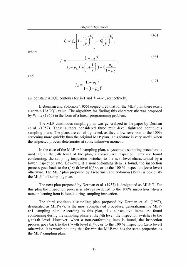
Olgierd Hryniewicz

18

31

1

31

111

+

−≈ ∞

kf

kffk ,

(43)

where

( )

( ) ( )L

Li

iL

iL

p

pi

ip

pf

−+

++−

−=

11

111

11 ,

(44)

and

( )( )iL

iL

p

pf

−−

−=∞

11

1

(45)

are constant AOQL contours for k=1 and ∞→k , respectively.

Lieberman and Solomon (1955) conjectured that for the MLP plan there exists

a certain UAOQL value. The algorithm for finding this characteristic was proposed

by White (1965) in the form of a linear programming problem.

The MLP continuous sampling plan was generalized in the paper by Derman

et al. (1957). These authors considered three multi-level tightened continuous

sampling plans. The plans are called tightened, as they allow reversion to the 100%

screening more quickly than the original MLP plan. This feature is very useful when

the inspected process deteriorates at some unknown moment.

In the case of the MLP-r×1 sampling plan, a systematic sampling procedure is

used. If, at the j-th level of the plan, i consecutive inspected items are found

conforming, the sampling inspection switches to the next level characterized by a

lower inspection rate. However, if a nonconforming item is found, the inspection

process goes back to the (j-r)-th level if j>r, or to the 100 % inspection (zero level)

otherwise. The MLP plan proposed by Lieberman and Solomon (1955) is obviously

the MLP-1×1 sampling plan.

The next plan proposed by Derman et al. (1957) is designated as MLP-T. For

this plan the inspection process is always switched to the 100% inspection when a

nonconforming item is found during sampling inspection.

The third continuous sampling plan proposed by Derman et al. (1957),

designated as MLP-r×s, is the most complicated procedure, generalizing the MLP-

r×1 sampling plan. According to this plan, if i consecutive items are found

conforming during the sampling phase at the j-th level, the inspection switches to the

(j+s)-th level. However, when a non-conforming item is found, the inspection

process goes back to the (j-r)-th level if j>r, or to the 100 % inspection (zero level)

otherwise. It is worth noticing that for r=s the MLP-r×s has the same properties as

the MLP sampling plan.


19

Derman et al. (1957) derived the following formula for the average fraction

inspected F(p) for the MLP-T tightened plan

( ) ( ) pq,f

q

fq

fq

qpF

ki

i

ki

i −=

+

−

−

−= 1

1

1

11

.

(46)

They also found closed-form formulae for the values of AOQL, but only for the case

of an infinite number of inspection levels. In the case of the MLP-r×1 sampling plan,

the AOQL is given by the following expression

i

r

r

f

ffAOQL

1

1

1

11

−

−−=

+

+,

(47)

and by

ifAOQL1

1−= (48)

in the case of the MLP-T sampling plan. Additional variants of the MLP-T sampling

plan were proposed by Guthrie and Johns (1958) who considered alternative

sequences of sampling rates.

In the case of an unstable process, the value of AEDL of this plan was found

by Hillier (1964) and is given by the following formula

( )

≤

>−

−−−

=

00

0111

x,

x,xpff

f

AEDL L

xk

k

k

,

(49)

where

( ) ( )( )k

kkL

k

fln

flnf

pfln

x−

−−

−

=1

11.

(50)

Multi-level continuous sampling plans like MLP or MLP-T do not allow an

immediate switch to low sampling rates when the history of screening shows good

quality of the inspected process. Sackrowitz (1972) proposed alternative multi-level

plans that are fully equivalent to the MLP or MLP-T plans (i.e. they have the same

statistical characteristics in case of stable quality of the inspected process), but allow

a return to a high sampling level more quickly than can be done in the case of the

MLP or MLP-T plans. In the plans proposed by Sackrowitz (1972), 100% inspection

is switched to sampling when i consecutive conforming items are found, but in

contrast to MLP and MLP-T plans, the type of sampling inspection that follows the

Olgierd Hryniewicz

20

screening phase depends on the length of time that is needed for switching to the

sampling phase.

In case of the sampling plan, designated by Sackrowitz (1972) P*, which is

fully equivalent to the MLP-T sampling plan, the switching rules are the following:

1) If the first i items inspected during the initial screening phase are found

conforming, switch to the second level of sampling characterized by the

sampling rate f2. Otherwise, when i consecutive items inspected during the

initial screening phase are found conforming, switch to the first level of

sampling characterized by the sampling rate f1> f2.

2) When on fi , i=1,…,m, sampling inspection level, continue sampling until a

nonconforming item is found. When it occurs, revert immediately to 100%

screening. If the first i items inspected during this screening phase are found

conforming, switch to the j*, j

*=min(j+1,m) level of sampling, characterized

by the sampling rate ∗jf . Otherwise, when i consecutive items inspected

during this screening phase are found conforming, switch to the first level of

sampling, characterized by the sampling rate f1.

In case of the sampling plan designated by Sackrowitz (1972) P**

, which is

fully equivalent to the MLP sampling plan, the switching rules are rather

complicated, and this feature limits the practicability of this plan.

Probably the most general multi-level continuous sampling procedure has

been proposed by Sakamoto and Kurano (1978). These authors propose finding

optimal values of the parameters of that procedure using a very complicated model of

a stochastic game.

4. Continuous sampling plans of the WSP-type

Wald and Wolfowitz (1945) in their seminal paper noticed that Dodge’s CSP

sampling plan does not assure a prescribed AOQL level when the quality of the

inspected process varies in time. In order to avoid this problem, they proposed a

sampling procedure, labeled in their paper SPC, which later on has been designated

WSP-1. The WSP-1 sampling plan is based on a concept different from the CSP

sampling plans, and the plans based on this concept are called the WSP-type

sampling plans. In the case of the WSP-type continuous sampling plans the inspected

process is divided into groups of N items each. These groups, if needed, may be

diverted from the original process for further screening. Therefore, the WSP-type

sampling plans may be regarded as rectification procedures for batches of N items

each.

In the original WSP-1 sampling plan the group of N items is divided into n

segments of 1/f items each. For each of the groups, inspection begins by sampling

one item taken at random from consecutive segments. This sampling phase is

continued until c+1 nonconforming items are found or until all the segments have

been sampled. If the (c+1)st nonconforming item is found in the j

th segment, the


21

remaining n-j segments are diverted to 100% screening, and sampling of the next

group of N items begins.

Wald and Wolfowitz (1945) proved that the parameter c is the smallest integer

that fulfills the inequality

( )( )AOQL

n

fc>

−+ 11.

(51)

Shahani (1979) investigated other properties of the WSP-1 sampling plan. He

showed that the proportion of inspected items, both in sampling and screening

phases, is given by the following expression

( ) ( )

+−−= ∑+=

n

cj

ja jPn

c,nPfF

1

11

11 ,

(52)

where

( ) ∑+=

−=n

cj

ja Pc,nP

1

1 , (53)

and

( ) njc,ppc

jP

cjcj ≤≤+−

−= −−+

111 11

. (54)

Then, Shahani (1979) also showed that the AOQ function

( ) ( )11 FppAOQ −= (55)

for the WSP-1 sampling plan is an increasing function, attaining its maximum at p=1.

This maximum is equal to the value of (unrestricted) AOQL in (51). Therefore, the

WSP-1 sampling plan in the most unfavorable condition does not provide protection

against bad quality.

Read and Beattie (1961) modified the WSP-1 procedure, and proposed a plan,

named later WSP-2. According to the WSP-2 plan, when the (c+1)st nonconforming

item is found in the jth

segment, all the j sampled segments are diverted for screening

and the count of a new group of N items begins. The proportion of inspected items

for the WSP-2 plan is given, using the notation of Shahani (1979), by

( ) ( )

( ) ∑+=

+

−−=

n

cj

ja

a

jPn

c,nP

c,nPfF

1

21

11 .

(56)

The AOQ function of the WSP-2 sampling plan, calculated according to (55)

with F2 replacing F1, has one maximum. Therefore, this plan does not have the

Olgierd Hryniewicz

22

unsatisfactory property of the WSP-1 plan, mentioned above. On the other hand, the

properties of this plan in the case of quality varying in time are not known.

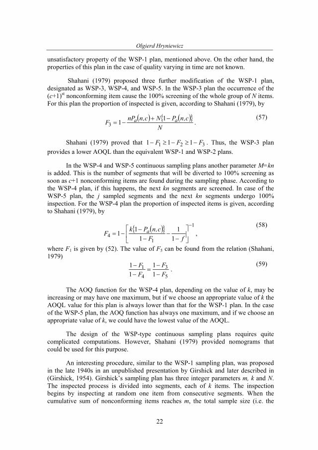
Shahani (1979) proposed three further modification of the WSP-1 plan,

designated as WSP-3, WSP-4, and WSP-5. In the WSP-3 plan the occurrence of the

(c+1)st nonconforming item cause the 100% screening of the whole group of N items.

For this plan the proportion of inspected is given, according to Shahani (1979), by

( ) ( ){ }N

c,nPNc,nnPF aa −+

−=1

13 . (57)

Shahani (1979) proved that 321 111 FFF −≥−≥− . Thus, the WSP-3 plan

provides a lower AOQL than the equivalent WSP-1 and WSP-2 plans.

In the WSP-4 and WSP-5 continuous sampling plans another parameter M=kn

is added. This is the number of segments that will be diverted to 100% screening as

soon as c+1 nonconforming items are found during the sampling phase. According to

the WSP-4 plan, if this happens, the next kn segments are screened. In case of the

WSP-5 plan, the j sampled segments and the next kn segments undergo 100%

inspection. For the WSP-4 plan the proportion of inspected items is given, according

to Shahani (1979), by

( ){ } 1

14

1

1

1

11

−

−−

−−

−=fF

c,nPkF a ,

(58)

where F1 is given by (52). The value of F5 can be found from the relation (Shahani,

1979)

5

3

4

1

1

1

1

1

F

F

F

F

−−

=−−

. (59)

The AOQ function for the WSP-4 plan, depending on the value of k, may be

increasing or may have one maximum, but if we choose an appropriate value of k the

AOQL value for this plan is always lower than that for the WSP-1 plan. In the case

of the WSP-5 plan, the AOQ function has always one maximum, and if we choose an

appropriate value of k, we could have the lowest value of the AOQL.

The design of the WSP-type continuous sampling plans requires quite

complicated computations. However, Shahani (1979) provided nomograms that

could be used for this purpose.

An interesting procedure, similar to the WSP-1 sampling plan, was proposed

in the late 1940s in an unpublished presentation by Girshick and later described in

(Girshick, 1954). Girshick’s sampling plan has three integer parameters m, k and N.

The inspected process is divided into segments, each of k items. The inspection

begins by inspecting at random one item from consecutive segments. When the

cumulative sum of nonconforming items reaches m, the total sample size (i.e. the


23

number of inspected segments) is compared to N. If Nn ≥ , the inspected process is

considered acceptable. Otherwise, the next N-n segments are screened.

For the plan proposed by Girshick (1954) the following inequality holds

N

mk

UAOQL

−

≤

11

.

(60)

This inequality can be used for choosing the parameters of the plan. Another

possibility proposed by Girshick (1954) is to use expressions for the variance of the

outgoing quality. Girshick’s procedure is the first application of a sequential

statistical test in the inspection of continuous processes. It has been extended by

Albrecht et al. (1955) who proposed to use Wald’s sequential sampling plan for

making decisions about switching from sampling to screening.

5. Other approaches to continuous sampling

Continuous sampling plans of CSP-type and WSP-type are not the only

sampling procedures that have been proposed for the inspection of continuous

processes. There exist continuous sampling plans that retain the original Dodge’s

idea of switching between screening and sampling, but use other statistical

procedures for making decisions for switching. There exist also procedures that do

not require explicitly the implementation of 100% screening. In this section we give

a short description of those of them which seem to be the most applicable in quality

control practice.

It seems to be quite obvious that a good inspection procedure should assure

quick switching from screening to sampling when the quality of inspected process is

good, and also quick switching from sampling to screening when the inspected

process deteriorates. Classical continuous sampling procedures with very simple

decision rules do not fulfill this requirement.

It is well known from the theory of mathematical statistics that decision

procedures based on sequential tests, such as cumulative sums (CUSUMS), are

characterized by shortest inspection runs before making decisions. Therefore, they

may be effectively used for the purpose of continuous inspection. Bourke (2002) has

proposed such a procedure, designated CSP-CUSUM sampling plan. He proposes to

use the same type of data as in the CSP-type procedures, namely run-lengths Yi, i=1,

2, …, between successive recorded non-conforming items. Decision for switching

from screening to sampling is made when the cumulative sum

[ ] 0210 01 ==−+= − G,,,i,kYG,MaxG iii K (61)

is equal or greater than a prescribed number hc. Let pa be an acceptable quality level

for which sampling inspection is advisable, and pr be a rejectable quality level for

which 100% screening is needed. From the theory of sequential probability ratio tests

(SPRT) one can find the formula for the choice of the parameter k to be

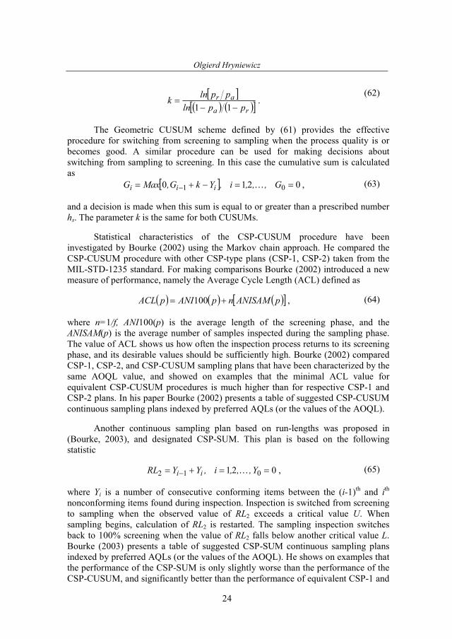
Olgierd Hryniewicz

24

[ ]( ) ( )[ ]ra

ar

ppln

pplnk

−−=

11.

(62)

The Geometric CUSUM scheme defined by (61) provides the effective

procedure for switching from screening to sampling when the process quality is or

becomes good. A similar procedure can be used for making decisions about

switching from sampling to screening. In this case the cumulative sum is calculated

as

[ ] 0210 01 ==−+= − G,,,i,YkG,MaxG iii K , (63)

and a decision is made when this sum is equal to or greater than a prescribed number

hs. The parameter k is the same for both CUSUMs.

Statistical characteristics of the CSP-CUSUM procedure have been

investigated by Bourke (2002) using the Markov chain approach. He compared the

CSP-CUSUM procedure with other CSP-type plans (CSP-1, CSP-2) taken from the

MIL-STD-1235 standard. For making comparisons Bourke (2002) introduced a new

measure of performance, namely the Average Cycle Length (ACL) defined as

( ) ( ) ( )[ ]pANISAMnpANIpACL += 100 , (64)

where n=1/f, ANI100(p) is the average length of the screening phase, and the

ANISAM(p) is the average number of samples inspected during the sampling phase.

The value of ACL shows us how often the inspection process returns to its screening

phase, and its desirable values should be sufficiently high. Bourke (2002) compared

CSP-1, CSP-2, and CSP-CUSUM sampling plans that have been characterized by the

same AOQL value, and showed on examples that the minimal ACL value for

equivalent CSP-CUSUM procedures is much higher than for respective CSP-1 and

CSP-2 plans. In his paper Bourke (2002) presents a table of suggested CSP-CUSUM

continuous sampling plans indexed by preferred AQLs (or the values of the AOQL).

Another continuous sampling plan based on run-lengths was proposed in

(Bourke, 2003), and designated CSP-SUM. This plan is based on the following

statistic

021 012 ==+= − Y,,,i,YYRL ii K , (65)

where Yi is a number of consecutive conforming items between the (i-1)th

and ith

nonconforming items found during inspection. Inspection is switched from screening

to sampling when the observed value of RL2 exceeds a critical value U. When

sampling begins, calculation of RL2 is restarted. The sampling inspection switches

back to 100% screening when the value of RL2 falls below another critical value L.

Bourke (2003) presents a table of suggested CSP-SUM continuous sampling plans

indexed by preferred AQLs (or the values of the AOQL). He shows on examples that

the performance of the CSP-SUM is only slightly worse than the performance of the

CSP-CUSUM, and significantly better than the performance of equivalent CSP-1 and


25

CSP-2 plans. Taking into account its simplicity, the CSP-SUM should be regarded as

a valuable option for the inspection of continuous processes.

An original, and easily implemented, continuous sampling procedure was

proposed by Beattie (1962). Beattie’s procedure is the application of two CUSUM

control charts. Samples of n items each are taken from an inspected process, and the

numbers of nonconforming items, di, i=1,2,…are used for the calculation of

cumulative sums

[ ] 0210 01 ==−+= − S,,,i,kdS,MaxS iii K , (66)

where k is a reference value proportional to the slope of Wald’s sequential sampling

plan. Charting is continued in the accept zone as long as Si<h, where h is a parameter

of the chart. If hSi ≥ , the procedure is switched to the reject zone, and the CUSUM

plot is moved up to the value h+h*. The charting is continued in the reject zone,

using cumulative sums

[ ]kdS,hhMinS iii −++= −∗

1 , (67)

until hSi ≤ . When hSi ≤ , the CUSUM plot is restarted at 0. In his paper Beattie

(1962) proposes to reject (i.e. to throw away, or put on side for 100% inspection if

desired) all produced items while the inspection process remains in the reject zone.

For the calculation of the characteristics of his procedure, Beattie (1962) used

a general methodology proposed for CUSUM charts by Ewan and Kemp (1960).

According to this methodology, two systems of linear equations have to be solved. In

the case of the CUSUM procedure in the accept zone we have to solve, with respect

to the function L(z,p) describing the expected number of inspected samples, the

following equations

( ) ( ) ( ) ( ) ( )∑ ∑−

=

−

=

−=+−++=1

1 0

11001h

y

zk

x

h,,,z,xp,Lzkyp,yLp,zL Kϕϕ .

(68)

In the case of the reject zone, a similar system is given by the following formula

( ) ( ) ( ) ( ) ( ) 110011

1

−=+−++= ∗−

=

∞

+=

∗∗∗ ∑ ∑∗

h,,,z,xp,Lzkyp,yLp,zLh

y kzx

Kϕϕ .

(69)

In both (68) and (69) ( )xϕ is the probability function, binomial or Poisson,

that depends on the fraction nonconforming p, and determines the probability of

observing in the sample of r items exactly x nonconforming items. The Average Run

Length in the accept zone ARL0, i.e. the expected number of inspected samples until

the process switches to the reject zone, is given by L(0,p). The same characteristic in

the reject zone, ARL1, is given by L*(0,p). When the sampling rate is the same in

Olgierd Hryniewicz

26

both zones, the OC curve, understood as the proportion, PA, of product accepted, for

a given quality p, is given by

( ) ( )( ) ( )p,Lp,L

p,LpPA

00

0∗+

= . (70)

The graphs of ARLs in both zones were presented by Prairie and Zimmer

(1973) for different combinations of n, k, h and h*. These graphs can be used for the

determination of these parameters, i.e. for the design of Beattie's procedure.

It is worth noting that Beattie (1962) leaves the problem of the frequency of

sampling open. Therefore, his procedure cannot be directly compared to other

continuous sampling procedures. Zimmer and Tai (1980) considered the case when

the sampling rate (i.e. the proportion of sampled items) in the acceptance zone is

equal to ra, and the sampling rate in the reject zone is equal to rr. If rr<1 (i.e. less than

100% items are inspected in that zone), and rr>ra, the average fraction of total

product inspected in the long run is (Zimmer and Tai, 1980)

( ) ( ) ( )( ) ( )p,L

rp,L

r

p,Lp,LpF

ra

01

01

00

∗

∗

+

+= .

(71)

Hence, the AOQ function is given by

( ) ( ) ( )ppPrrprAOQ Aarr −+−= 1 . (71)

where f=ra/rr, and the probability of acceptance Pa(p) is given by

( ) ( )( ) ( )p,fLp,L

p,LpPA

00

0∗+

= . (72)

When rr=1, or when rr<1 but the rejected material is diverted for 100% screening, the

AOQ function is given by

( ) ( )ppPrAOQ Aa−= 1 . (73)

In both cases considered above, Pa(p) is computed with rr=1.

Zimmer and Tai (1980) showed that slightly modified Dodge's CSP-1 and

CSP-2 continuous sampling plans are special cases of the Beattie procedure. Suppose

that the Beattie procedure begins in the reject zone, i.e. S0=h+h*. If we take n=1, rr=1,

ra=f, k=1/i, h=1-1/i, and h*=1, the Beattie procedure is the same as the CSP-1

sampling plan. Moreover, when we set n=1, rr=1, ra=f, k=1/(l+1), h=1, and

h*=i/(l+1), where l is the release parameter in the sampling phase of the CSP-2

sampling plan, the Beattie procedure is the same as the CSP-2 sampling plan. Thus,

CSP-1 and CSP-2 are special cases of Beattie’s procedure for sampling by attributes.


27

Beattie’s procedure is a combination of two CUSUM procedures. Thus, it can

be used not only for sampling by attributes, but – as was already noticed by Beattie

(1962) – also for sampling by variables. Wasserman and Wadsworth in their papers,

Wadsworth and Wasserman (1987) and Wasserman and Wadsworth (1989)

considered a general case when monitored quality characteristic is distributed

according to the probability distribution that belongs to the general family of the

exponential distributions (Darmois-Koopman family) defined by the pdf function

( ) ( ) ( ) ( ) ( )[ ]xTDexpxaC;xf θθθ = , (74)

where ( ) 0>θC , ( ) 0>xa , and ( )θD is a strictly increasing function of θ . It is well

known that the popular SQC probability distributions such as the binomial, Poisson

and normal belong to this family.

Statistical properties of Beattie’s procedure can be analyzed using general

results presented in Wald (1947). Results of this analysis for the general case are

given in Wadsworth and Wasserman (1987). Let 0θ represent the good process

quality level, and 1θ represent the bad process quality level. The SPRT reference

parameter k (the reference parameter of the CUSUM procedure) according to Wald’s

theory should be computed from the following formula

( ) ( )[ ]D

CClnk

∆θθ 10= ,

(75)

where ( ) ( )01 θθ∆ DDD −= . Let ( )θg be the function satisfying the famous Wald’s

identity

( )[ ] 1=θθ |SgE NX , (76)

where SN is the SPRT statistic upon termination of the test. Wasserman has shown,

see Wadsworth and Wasserman (1987) for detailed information, that the Average

Run Length of Beattie’s procedure in the accept zone is given by

( ) ( )

−−+

−=

ηη

θθ

11

exp

k

hL ,

(77)

where ( )θ∆η Dgh−= . Similarly, in the reject zone the ARL function is given by

( ) ( )

−−+−

−=

∗

∗∗∗

η

ηθ

θ1

1exp

k

hL ,

(78)

where ( )θ∆η Dgh∗−= . In the derivation of (77) and (78) it is assumed that the

reference value k is the same for both zones.

Olgierd Hryniewicz

28

Read and Beattie (1961) introduced the Type C OC curve for continuous

acceptance sampling as the long run proportion of product that is accepted. The

approximate expression for this characteristic was given in Wadsworth and

Wasserman (1987)

( ) ( )( ) ( ) 0

2

1≠

+−+−−

−+−≈ ∗

∗∗ηη

ηηηη

ηηθ ,,

expexp

expPa .

(79)

This characteristic has been used in Wadsworth and Wasserman (1987) for designing

Beattie’s procedure.

Wasserman, see Wadsworth and Wasserman (1987), has shown that Beattie’s

procedure with k=k* and h=h

* (i.e. with ∗= ηη ) gives the best “discrimination”

between processes described by 0θ and 1θ , respectively. This discrimination is

measured by the difference ( ) ( )10 θθ aa PP − . Thus, Wadsworth and Wasserman

(1987) used this assumption for the construction of the procedure. They also assumed

that for the process of “good” quality, characterized by the parameter 0θ , the

fraction of accepted product should be greater than 1-α. On the other hand, for the

process of “bad” quality, characterized by the parameter 1θ , the fraction of accepted

product should be smaller than β. Moreover, they assumed that the average number

of samples inspected in the reject zone, if the process is “good”, should be smaller

than L0. On the other hand, the average number of samples inspected in the accept

zone, if the process is “bad”, should be smaller than L1. In case of sampling by

attributes (described by the Poisson distribution) the algorithm proposed in

Wadsworth and Wasserman (1987) is the following:

1) Specify L0, L

1, 0θ , 1θ , α, β.

2) Calculate k from

−=

0

1

01

θθ

θθ

ln

k

3) Find η0 from ( ) αη −≥ 10aP , and η1 from ( ) βη ≤1aP .

4) Let ηmax=max{η1,−η0}.

5) Calculate h from

=

2

1θ

θη

ln

h max .

6) Calculate the sample size n as the smallest integer not smaller than

−=∗

1001

112

L,

Lmax

hn

θθ.


29

The detailed description of this procedure in the case of the normal

distribution is given in Wasserman and Wadsworth (1989) for θ0=µ0, θ1=µ1, known

σ2, and L

1=L

0.

1) Specify L0, µ0, µ1, σ

2, α, β.

2) Let k=0,5(µ0+µ1).

3) Find η0 from ( ) αη −≥ 10aP , and η1 from ( ) βη ≤1aP .

4) Let ηmax=max{η1,−η0}.

5) Let

001

2Lh

µµ −= .

6) For item-by-item sampling, verify that

0

201 2

L

maxησ

µµ≥

−;

otherwise, choose n as the nearest integer to quantity

( )01

2

µµησ−h

max .

6. Economically optimal procedures for monitoring continuous processes

Every implementation of sampling inspection has some economic

consequences. In the case of sampling of continuous processes one can distinguish

two general cases: “troubleshooting” (Chiu and Wetherill, 1973), and product

screening. The aim of product screening is simply to rectify the process. The

“troubleshooting” is used to determine if the process has deteriorated. It is usually

assumed that a continuous process may be either in a “good” state (state 1) or in a

“bad” state (state 2). The transition from the “good” state to a “bad” one is not

directly observed, and can be revealed by an appropriate sampling procedure. When

the process is judged to be in a “bad” state it has to be stopped, and the search for an

assignable cause of this situation should begin. It is also assumed that a deteriorated

process cannot be improved without some repair actions.

The first attempt to use an economic approach in the design of a continuous

sampling procedure was proposed in the paper by Girshick and Rubin (1952). They

assumed that after each item produced in state 1 there is a constant probability, p, that

the process will jump to state 2. It is assumed that the quality characteristic X has the

probability distribution f1(x) when the process is in state 1, and the probability

distribution f2(x) when the process is in state 2. Moreover, it is assumed that the value

of the item of quality x is V(x). When the process is stopped in state i (i=1,2), it takes

ni time units (a time unit is taken to be the time of the production of one item) for

inspection and repairing, and the costs of these actions per time unit are equal to ci

(i=1, 2).

Olgierd Hryniewicz

30

Girshick and Rubin (1952) considered two cases. In the first one they assumed

that the cost of sampling is negligible, and thus the 100% inspection is used. They

applied a Bayesian approach and showed that the optimum stopping rule is to stop

the process if after the inspection of the kth

item the condition aZk ≥ , where

( )10 10 −+== kkk ZyZ,Z , (80)

and

( )( ) ( )k

kk

xfp

xfy

1

2

1−= ,

(81)

is fulfilled. The critical value a can be found by solving an integral equation and then

maximizing the average income.

In the second case that they considered, Girshick and Rubin (1952) assumed

that the inspection process is costly. In this case the optimum rule is also defined in

terms of Zk calculated according to (80), but the value yk is now calculated as

pyk −

=1

1.

(82)

The decision rule is now the following: produce the next item without inspection if

Zk<b, inspect the next produced item if aZb k <≤ , and stop the process if aZk ≥ .

The critical values a, and b are calculated in a similar way as in the first case

mentioned above. The results of Girshick and Rubin (1952) have been generalized by

many other authors. Some information about those results can be found in Chiu and

Wetherill (1973).

When a process is characterized by a constant probability of producing a

nonconforming item, and functions describing costs of inspection, repair or

replacement, and costs of passing a nonconforming item are linear, then the

economically optimal procedure is either to inspect all items (100% screening) or to

do nothing. The first option is optimal when Bpp ≥ , and the second option is

optimal when Bpp ≤ , where pB is a certain quality level, called “break-even

quality”. This result was firstly proved for the inspection of lots, see Hald (1981) for

more information, and later for the inspection of continuous processes. Vander Wiel

and Vardeman (1994) have shown that this result is valid for a more general model of

process behavior. Therefore, sampling inspection of continuous processes may be

optimal only in the case of quality p that varies in time around the value of pB.

Anscombe (1958) was the first author who used a cost model for finding an

optimal procedure of the CSP type. Let s be the cost of passing a nonconforming

item, r be the cost of repair or replacement of a nonconforming item found during the

inspection, and c be the unit cost of inspection, and

rs

cpk B −

== (83)

be the “break-even quality”.


31

Anscombe (1958) made the following additional assumptions:

a) On the average, the process deteriorates after M items have been

produced;

b) Process quality p varies randomly according to a uniform distribution

in the range (0, 2k);

c) The fraction of items inspected at k is equal to 0.5, i.e. F(k)=0.5.

Using these assumptions he found that the optimal parameters of the CSP-1 plan can

be calculated from the formulae

( ) 32

30−= kM,f ,

(83)

and

( )

≈

−

−=

fln

ppln

f

fln

iBB

11

1

1.

(84)

The results obtained by Anscombe (1958) can be justified using the mini-max

approach to optimization of sampling procedures. Let V(p) be the expected cost per

unit produced that includes costs of inspection, costs of repair or replacement of

nonconforming items found during inspection, and costs (losses) due to passing

nonconforming items. The costs described by V(p) consist of two parts, and one of

them U(p) describes costs that are unavoidable for any inspection procedure. The

difference

( ) ( ) ( )pUpVpR −= (85)

is called the regret function, and describes additional costs related to the applied

inspection procedure. The mini-max approach for the design of a sampling procedure

consists in finding such parameters of this procedure for which the function

( ) ( )pRmaxpRp 10 ≤≤

∗ = (86)

is minimized. Thus, a mini-max optimal procedure guarantees the lowest costs in the

most unfavorable situation.

The first paper devoted to the problem of the mini-max optimization of the

CSP-1 continuous sampling plan was published by Ludwig (1974). He proposed the

following cost function

( ) ( ) ( )pFbpacpV ++= , (87)

where c is the average cost of producing an item (the average profit from a produced

item, if c is negative), a is the cost of inspection of one item, b is the cost of repair or

replacement of a nonconforming item found during the inspection, and F(p) is the

fraction of inspected items. Moreover, Ludwig (1974) assumed that the sampling

Olgierd Hryniewicz

32

procedure should assure that the average outgoing quality should not be worse than

L1. Then, he defined the regret function as

( ) ( ) ( )( ) ( )[ ]

≤<+−+

≤≤+=

11

0

11

1

pLpLpFbpa

LppFbpapR

(88)

The mini-max optimal plans for this regret function have been tabulated in Ludwig

(1974) for different combinations of L1 and d=a/b.

Another mini-max model for the optimization of the CSP-1 plan has been

proposed by Vogt (1986). He assumed a typical cost model

( ) ( ) ( ) pspFpsbpapV +−+= , (89)

where costs a and b are the same as in the model by Ludwig (1974), and s is the cost

of passing a nonconforming item. The standardized regret function proposed by Vogt

(1986) is described by the following formula

( ) ( ) ( )( ) ( )[ ]

≤<−−

≤≤−=

11

0

pppFpp

pppFpppR

BB

BB.

(90)

For this regret function Vogt (1986) proposed an algorithm for finding approximately

mini-max optimal parameters of the CSP-1 plan.

In the classical approach to the economic optimization of sampling procedures

used in lot-by-lot inspection it is assumed that quality varies randomly from lot to lot.

This approach can be applied in the case of plans of the CSP-type if we assume that

the inspected process is divided into many segments of finite and long length, and the

quality varies randomly from segment to segment. This approach is described in the

paper by Hryniewicz (1988). The optimal results are characterized by large values of

the release parameter i, and the very small values of the sampling rate f. This result is

hardly unexpected. The role of the first screening period is to verify if the quality is

better than the “break-even quality”. If it is so, the further inspection is not necessary.

Otherwise, the whole segment should be screened.

7. Continuous sampling plans in standards

The first standards on continuous sampling plans were published in the US

Department of Defense in the 1950s (H-106, H-107). Another standard of that type

(QSTAG 340) was developed together for the Armies of the United States, the

United Kingdom, Canada and Australia in the 1970s. The most popular standard,

developed as the successor to H-106 and H-107, was published under designation

MIL-STD-1235A in 1974. Its latest version, MIL-STD-1235C (1988), is now

available on the Web free of charge.


33

MIL-STD-1235C (1988) provides tables, figures, and procedures for five

types of continuous sampling plans by attributes:

• CSP-1 continuous sampling plans;

• CSP-F continuous sampling plans for finite production runs;

• CSP-T three-level continuous sampling plans ;

• CSP-2 continuous sampling plans;

• CSP-V continuous sampling plans (similar to CSP-2 and CSP-3

sampling plans).

Sampling plans in MIL-STD-1235C are indexed by Sampling Frequency Code Letter

that determines parameter f of the plan, and Acceptable Quality Level (AQL) which

for continuous sampling plans is simply an index, and does not have any precisely

defined meaning.

Recommended sampling frequencies form a series of preferred frequencies

from 1/2 (code letter A), to 1/200 (code letter K). The choice of an appropriate code

letter depends upon the number of units in a production interval that shall not be

longer than one day’s production.

Clearance numbers, i, are chosen from tables for given pairs of code letter and

AQL. In sampling plans of MIL-STD-1235C the length of the screening phase is

limited by a constant S, i.e. when the number of items inspected during the screening

phase reaches S, inspection is suspended and corrective actions shall take place.

The operation procedures of CSP-1 and CSP-2 plans are the same as has been

presented in sections 2.1 and 2.2, respectively. The three-level CSP-T sampling plan

operates similarly as the original CSP-T plan described in section 3, but the sampling

frequencies on the consecutive levels are f, f/2, and f/4, instead of f, f2, and f

3. The

operation procedure of the CSP-F sampling plan is exactly the same as in the case of

the CSP-1 sampling plan. However, its parameters have been calculated under the

assumption of the finite length of production runs. CSP-F sampling plans are

organized in tables indexed by AQL and AOQL values. Possible finite production

runs have been divided into 32 non-overlapping intervals. In a given table for each of

these intervals eight sampling plans (i,f) are available. CSP-V sampling plan operates

like the CSP-2 sampling plan. However, when a second nonconforming item is found

during the sampling phase, additional 100% inspection of consecutive k items is

invoked (as in the CSP-3 plan). The procedure is switched to the screening phase

when a nonconforming item is found during this 100% inspection. Otherwise, the

sampling is continued as in the CSP-2 plan.

MIL-STD-1235C has over 300 pages, and on over 200 of them different

curves describing statistical characteristics of proposed plans (except for CSP-F

plans), such as e.g. AOQ curves, are given.

8. Future work on new standards for continuous sampling plans

Statistical procedures proposed in standards should fulfill certain important

requirements. First of all, they should be based on a firm mathematical basis.

Olgierd Hryniewicz

34

Secondly, they should be easily implemented in practice. And finally, they should

use similar language to that used by practitioners who work with their predecessors

or other similar standards. Future new standards on acceptance sampling of

continuous processes should definitely fulfill these requirements.

Classical standardized acceptance sampling plans are used at an interface

between a “producer” and a “user”. Therefore, the amount of information that is

needed for their design and further implementation should be limited to that available

by both “partners”. This seems to be very restrictive in many practical cases, and –

for example – limits the possibility of using economic considerations in construction

of sampling procedures. In contrast to that, continuous sampling may be mainly used

inside the same organization which is able to collect information of a confidential

character. Therefore, in future standardized procedure we should use the results

presented in section 6 showing that in case of stable processes the economically

optimal behaviour of the process owner is either to screen 100% of produced items or

to do nothing. Hence, the main aim for using such procedure is to confirm that the

inspected process is in a “good” state, and to indicate as quickly as possible that it

has just deteriorated and needs repair. In order to do so we need to introduce in a

standard the concept of the “break-even quality”. To do so, we propose to use the

concept of interval evaluation of unit costs.

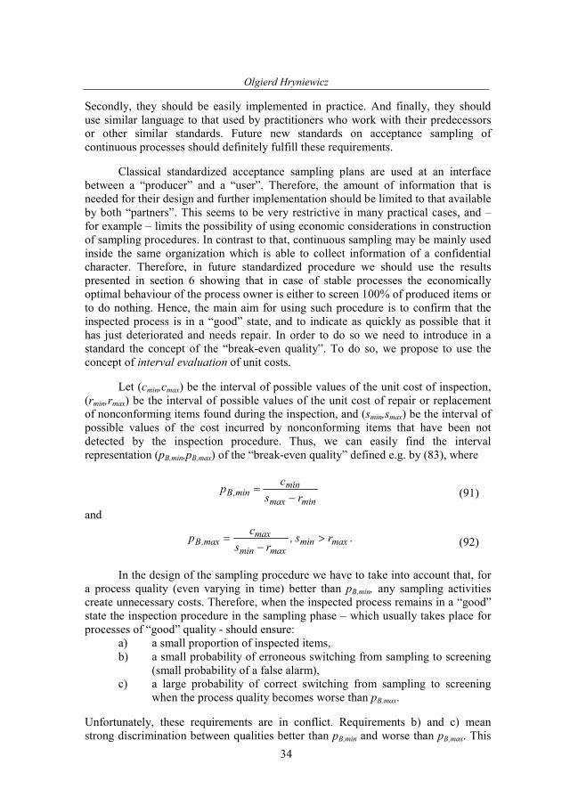
Let (cmin,cmax) be the interval of possible values of the unit cost of inspection,

(rmin,rmax) be the interval of possible values of the unit cost of repair or replacement

of nonconforming items found during the inspection, and (smin,smax) be the interval of

possible values of the cost incurred by nonconforming items that have been not

detected by the inspection procedure. Thus, we can easily find the interval

representation (pB,min,pB,max) of the “break-even quality” defined e.g. by (83), where

minmax

minmin,B

rs

cp

−=

(91)

and

maxminmaxmin

maxmax,B rs,

rs

cp >

−= .

(92)

In the design of the sampling procedure we have to take into account that, for

a process quality (even varying in time) better than pB,min, any sampling activities

create unnecessary costs. Therefore, when the inspected process remains in a “good”

state the inspection procedure in the sampling phase – which usually takes place for

processes of “good” quality - should ensure:

a) a small proportion of inspected items,

b) a small probability of erroneous switching from sampling to screening

(small probability of a false alarm),

c) a large probability of correct switching from sampling to screening

when the process quality becomes worse than pB,max.

Unfortunately, these requirements are in conflict. Requirements b) and c) mean

strong discrimination between qualities better than pB,min and worse than pB,max. This


35

cannot be achieved without taking large samples, and this stands in conflict with the

requirement a). We face an only slightly different situation when the inspection

process operates in its screening phase. The sampling procedure should in this case

ensure a quick return to the sampling phase when the quality is or becomes “good”.

On the other hand, however, when the process is “bad”, the probability of switching

from screening to sampling should be small. Thus, in this case we also face the

problem of good discrimination between two close quality levels. The only

difference, when compared to the first case considered, is related to the fact that in

the “bad” state we are not afraid of inspecting large amount of items. In fact in this

state, 100% screening is the optimal inspection policy. However, we must take into

account that a process that remains in a “bad” state is completely unacceptable.

Therefore, the permanent phase of screening cannot be accepted, and when this

happens, the process should be stopped and the assignable cause of this situation

should be found and removed.

The requirements presented above show undoubtedly that the inspection

process should start, as in the Beattie procedure, from the sampling phase. In order to

have good discrimination with the lowest possible sampling effort we have to use

sequential sampling tests. Therefore, potential candidates for this purpose are

Beattie’s sampling procedure, i.e. an ordinary CUSUM, or Bourke’s CSP-CUSUM

continuous sampling plan, i.e. a geometric CUSUM for runs. When the inspection

process enters the screening phase, the optimal procedure is Wald’s curtailed

sequential sampling plan. In this case the decision of acceptance shall cause the

return to the sampling phase, and the decision of rejection should be equivalent to the

decision of either to stop the process or to continue the 100% screening.

Parameters of sampling plans can be calculated independently for both phases

of inspection. This gives additional degrees of freedom for the designer of the

procedure who can use some additional criteria for choosing the best one. The

concept of the ACL introduced by Bourke (2002) and defined by (64) can be used for

this purpose. It seems that maximization of

( )pACLminACLmin,Bpp

min≤

= (93)

could yield the procedure, which for “good” processes operates mainly in the

sampling phase. Another feature worthy considering is the discrimination level of the

procedure in question. The highest discrimination may be achieved if we require low

probabilities of false decisions for process qualities pB,min and pB,max. One can

decrease the discrimination rate, and therefore decrease the inspection effort, by

replacing pB,min with the average quality q of the process being in a “good” state.

The simplest possibility, however, is to use the results of Wasserman and Wadsworth

(1989) for Beattie’s procedure taking into account different sampling rates in both

phases of the inspection process.

References

Albrecht L., Gulde H., Maclean A, Thompson P. (1955) Continuous sampling at Minneapolis-

Honeywell. Industrial Quality Control, 12, 3, 4.

Olgierd Hryniewicz

36

Anscombe F.J. (1958) Rectifying inspection of continuous output. Journ. Amer. Statist.

Assoc., 53, 702-714.

Balamurali S., Kalyanasundaram M., Jun Chi-Hyuck (2005). International Journal of

Reliability and Safety Engineering, 12, 2, 75-93.

Beattie D.W. (1962) A continuous acceptance sampling procedure based upon a cumulative

sum chart for the number of defectives. Applied Statistics, 11, 3, 137-147.

Bourke P.D. (2002) A continuous sampling plan using CUSUMs. Journal of Applied

Statistics, 29, 8, 1121-1133.

Bourke P.D. (2003) A Continuous Sampling Plan Using Sums of Conforming Run-length.

Quality and Reliability Engineering International, 19, 53-66.

Belyaev Y. (1975) Probabilistic methods of sample control (in Russian), Nauka, Moscow.

Blackwell M.T.R. (1977) The Effects of Short Production Runs on CSP-1. Technometrics, 19,

259-263.

Chiu W.K., Wetherill G.B. (1973) The Economic design of Continuous Inspection

Procedures: A Review Paper. International Statistical Review, 41, 3, 357-373.

Derman C., Johns M.V., Lieberman, G.J. (1959) Continuous sampling procedures without

control. Annals of Mathematical Statistics, 30, 1175-1191.

Derman C., Littauer S.B., Solomon H. (1957) Tightened multi-level continuous sampling

plans. Annals of Mathematical Statistics, 28, 395-403.

Dodge H.F. (1943) A sampling inspection plan for continuous production. Annals of

Mathematical Statistics, 14, 264-279.

Dodge H.F., Torrey M.N. (1951) Additional continuous sampling inspection plans. Industial

Quality Control, 7, 5, 7-12.

Endres A.C. (1969) The computation of the unrestricted AOQL when defective material is

removed but not replaced. Journ. Amer. Statist. Assoc., 64, 665-668.

Ewan W.D., Kemp K.W. (1960) Sampling Inspection of Continuous Processes with No

Autocorrelation between Successive Results. Biometrika, 47, 363-380.

Girshick M.A. (1954) A sequential inspection plan for quality control. Technical Report No

14, Applied Mathematics and Statistics Laboratory, Stanford University.

Girshick M.A., Rubin H. (1952) A Bayes approach to a quality control model. Annals of


Govindaraju K., Kandasamy C. (2000) Design of generalized CSP-C continuous sampling

plan. Journal of Applied Statistics, 25, 4, 829-841.

Guthrie D., Johns Jr. M.V. (1958) Alternative sequences of sampling rates for tightened

multi-level continuous sampling plans. Technical Report No 36, Applied Mathematics

and Statistics Laboratory, Stanford University.

Hald A. (1981) Statistical Theory of Sampling Inspection by Attributes. Academic Press,

London.

Hillier F.S. (1964) New criteria for selecting continuous sampling plans. Technometrics, 6,

161-178.

Hryniewicz O. (1988) Optimization of CSP-1 screening procedures for finite lots. Economic

Quality Control, 6, 1, 3-10.

Lieberman G.J. (1953) A note on Dodge’s continuous inspection plan. Annals of


Lieberman G.J., Solomon H. (1955) Multi-level continuous sampling plans. Annals of


Ludwig R. (1974) Bestimmung kostenoptimaler Parameter fur den kontinuerlichen

Stichproben. Metrika, 21, 83-126.

McShane L.M., Turnbull B.W. (1991) Probability Limits on Outgoing Quality for Continuous

Sampling Plans. Technometrics, 33, 4, 393-404.


37

MIL-STD-1235C (1988) Military Standard. Single- and Multi-Level Continuous Sampling

Procedures and Tables for Inspection by Attributes. U.S. Government Printing Office,

Washington, DC.

Murphy R.B. (1959) Stopping rules with CSP-1 sampling inspection plans in continuous

production. Industrial Quality Control, 16, 5, 5-9.

Phillips M.J. (1969) A Survey of Sampling Procedures for Continous Production. Journal of

the Royal Statistical Society. Series A (General), 132, 2, 205-228.

Prairie R.R., Zimmer W.J. (1973) Graphs, tables and Discussion to Aid in the Design and

Evaluation of an Acceptance sampling Procedure based on Cumulative Sums. Journal

of Quality Technology, 5, 2, 58-66.

Read D.R., Beattie D.W. (1961) Variable lot size acceptance sampling plan for continous

production. Applied Statistics, 10, 147-156.

Sackrowitz H. (1972) Alternative multi-level continuous sampling plans, Technometrics, 14,

3, 645-652.

Sakamoto T., Kurano M. (1978) Stochastic game models for the determination of the optimal

continuous sampling inspection plans. Bulletin of Mathematical Statistics, 18, 1-2, 9-

19.

Shahani A.K. (1979) Wald-Wolfowitz type sampling plans for continuous production.

Technometrics, 21, 1, 21-31.

Shor Y.B., Pakhomov A.A. (1973) Methods for the choice of a continuous sampling plan by

attributes (in Russian). Nadezhnost i kontrol kachestwa, No.1(1973), 10-22.

Vogt H. (1986) Application of the minimax-regret principle to continuous sampling.

Statistische Hefte, 27, 279-296.

Wadsworth H.M., Wasserman G. (1987) A Modified CUSUM Procedure as a Continuous

Sampling Scheme. In: H.-J. Lenz, G.B. Wetherill, P.-Th. Wilrich (Eds.) Frontiers in

Statistical Quality Control 3, Physica-Verlag, Heidelberg, 179-195.

Wald A. (1947) Sequential Analysis. Dover Publications, New York.

Wald A., Wolfowitz W. (1945) Sampling inspection plans for continuous production which

insure a prescribed limit on the outgoing quality. Annals of Mathematical Statistics,

16, 30-49.

Wasserman G.S., Wadsworth H.M. (1989) A Modified Beattie Procedure for Process

Monitoring. Technometrics, 31, 4, 415-421.

White L.S (1965) Markovian decision models for the evaluation of a large class of continuous

sampling inspection plans. Annals of Mathematical Statistics, 36, 1408-1420.

White L.S (1966) The evaluation of H106 continuous sampling plans under the assumption of

worst conditions. Journal of the American Statistical Association, 61, 833-841.

Yang G.L. (1983) A Renewal-Process Approach to Continuous Sampling Plan.

Technometrics, 25, 59-67.

Zimmer W.J., Tai Ch-Y. (1980) A General Continuous Sampling Plan for Controlling the

AOQ. Journal of Quality Technology, 12, 4, 191-195.

Olgierd Hryniewicz

38

ACCEPTANCE SAMPLING OF DISCRETE · PDF fileAcceptance sampling of discrete continuous...

Documents

Transcript of ACCEPTANCE SAMPLING OF DISCRETE · PDF fileAcceptance sampling of discrete continuous...