
University of Zielona Gora Faculty of Physics and … · Faculty of Physics and Astronomy Subject...
88
University of Zielona G ´ ora Faculty of Physics and Astronomy Subject matter: Physical Science Discipline: Physics Maciej Sznajder Degradation studies of materials under space conditions; under special emphasize of recombination processes. (Badanie proces´ ow degradacji materia l´ ow w warunkach przestrzeni kosmicznej, ze szczeg´ olnym uwzgl¸ ednieniem proces´ ow rekombinacji) Acceptance of supervisor: PhD thesis written under the supervision of: dr hab. Ulrich Geppert, prof. UZ Zielona G´ora, 2013
Transcript of University of Zielona Gora Faculty of Physics and … · Faculty of Physics and Astronomy Subject...
University of Zielona GoraFaculty of Physics and Astronomy
Subject matter: Physical ScienceDiscipline: Physics
Maciej Sznajder
Degradation studies of materials under space conditions; underspecial emphasize of recombination processes.
(Badanie procesow degradacji materia low w warunkach przestrzenikosmicznej, ze szczegolnym uwzglednieniem procesow rekombinacji)
Acceptance of supervisor: PhD thesiswritten under the supervision of:dr hab. Ulrich Geppert, prof. UZ
Zielona Gora, 2013

2
Contents
Abstract iii
1 Introduction 1
2 Interaction of the incident particles with matter 52.1 Total and differential cross section . . . . . . . . . . . . . . . . . . . . . . . . 52.2 Energy loss per unit length by ionization and excitation . . . . . . . . . . . . 82.3 Interactions of protons with matter . . . . . . . . . . . . . . . . . . . . . . . 9
2.3.1 Non-relativistic case . . . . . . . . . . . . . . . . . . . . . . . . . . . 102.3.2 Relativistic case . . . . . . . . . . . . . . . . . . . . . . . . . . . . . . 11
2.4 Recombination of electrons and protons to Hydrogen . . . . . . . . . . . . . 132.4.1 Auger recombination . . . . . . . . . . . . . . . . . . . . . . . . . . . 162.4.2 Resonant recombination . . . . . . . . . . . . . . . . . . . . . . . . . 212.4.3 Oppenheimer - Brinkman - Kramers (OBK) Process . . . . . . . . . . 242.4.4 Summary . . . . . . . . . . . . . . . . . . . . . . . . . . . . . . . . . 27
3 Degradation of materials under space conditions 313.1 An overview of degradation processes . . . . . . . . . . . . . . . . . . . . . . 31
3.1.1 Positive electric charging of foils due to irradiation . . . . . . . . . . 313.1.2 Sputtering - removal of the metallic foil ions by the incident particles 323.1.3 Atomic Oxygen - ATOX . . . . . . . . . . . . . . . . . . . . . . . . . 363.1.4 Electromagnetic radiation . . . . . . . . . . . . . . . . . . . . . . . . 37
3.2 Blistering . . . . . . . . . . . . . . . . . . . . . . . . . . . . . . . . . . . . . 393.2.1 Time evolution of bubble formation . . . . . . . . . . . . . . . . . . . 403.2.2 Experimental facts, space environment, and numerical analysis of bub-
ble formation . . . . . . . . . . . . . . . . . . . . . . . . . . . . . . . 433.2.3 Reflectivity of a metallic foil covered with bubbles . . . . . . . . . . . 48
4 Conclusions and Outlooks 51
A OBK recombination in metal lattices 53A.1 The Hartree approximation . . . . . . . . . . . . . . . . . . . . . . . . . . . 53A.2 The ionization energy of an electron in the 1s state - the OBK process . . . 54A.3 Cross section of the OBK process . . . . . . . . . . . . . . . . . . . . . . . . 55
B Formation of hydrogen molecular bubbles on metal surfaces 59B.1 Volume of a cap of a sphere . . . . . . . . . . . . . . . . . . . . . . . . . . . 59B.2 Helmholtz free energy of H2 molecules placed in certain positions in the sam-
ple’s lattice . . . . . . . . . . . . . . . . . . . . . . . . . . . . . . . . . . . . 59
i
ii CONTENTS
B.3 Helmholtz free energy of H atoms in the sample . . . . . . . . . . . . . . . . 60B.4 The derivatives of Helmholtz free energy of: gas of the ith bubble, metal de-
formation caused by the bubble, H2 molecules, and H atoms located outsidethe bubbles. . . . . . . . . . . . . . . . . . . . . . . . . . . . . . . . . . . . . 61
Acknowledgments 63
Table of Symbols 65
Table of Physical Constants 69
List of Figures 71
List of Tables 73
References 75
Abstract
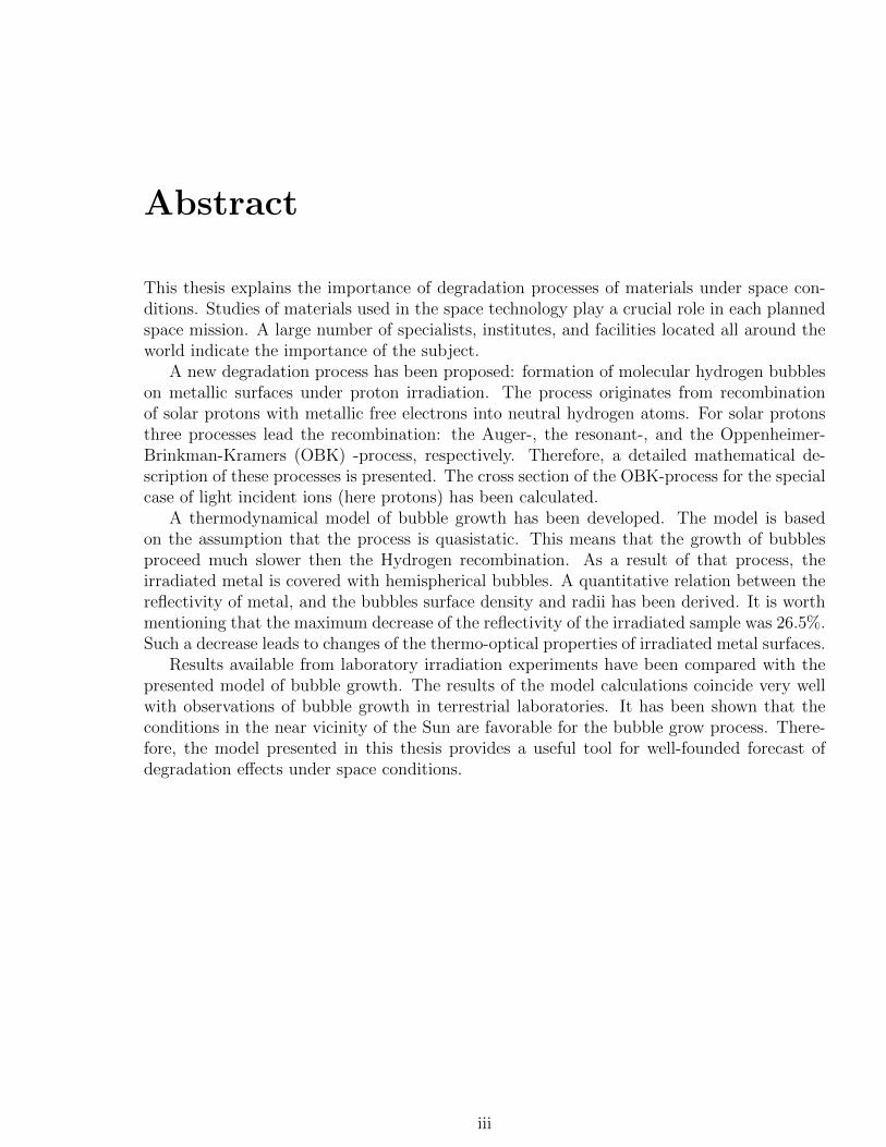
This thesis explains the importance of degradation processes of materials under space con-ditions. Studies of materials used in the space technology play a crucial role in each plannedspace mission. A large number of specialists, institutes, and facilities located all around theworld indicate the importance of the subject.
A new degradation process has been proposed: formation of molecular hydrogen bubbleson metallic surfaces under proton irradiation. The process originates from recombinationof solar protons with metallic free electrons into neutral hydrogen atoms. For solar protonsthree processes lead the recombination: the Auger-, the resonant-, and the Oppenheimer-Brinkman-Kramers (OBK) -process, respectively. Therefore, a detailed mathematical de-scription of these processes is presented. The cross section of the OBK-process for the specialcase of light incident ions (here protons) has been calculated.
A thermodynamical model of bubble growth has been developed. The model is basedon the assumption that the process is quasistatic. This means that the growth of bubblesproceed much slower then the Hydrogen recombination. As a result of that process, theirradiated metal is covered with hemispherical bubbles. A quantitative relation between thereflectivity of metal, and the bubbles surface density and radii has been derived. It is worthmentioning that the maximum decrease of the reflectivity of the irradiated sample was 26.5%.Such a decrease leads to changes of the thermo-optical properties of irradiated metal surfaces.
Results available from laboratory irradiation experiments have been compared with thepresented model of bubble growth. The results of the model calculations coincide very wellwith observations of bubble growth in terrestrial laboratories. It has been shown that theconditions in the near vicinity of the Sun are favorable for the bubble grow process. There-fore, the model presented in this thesis provides a useful tool for well-founded forecast ofdegradation effects under space conditions.
iii

iv CONTENTS

Streszczenie
Abstract in Polish.
v

vi CONTENTS
Chapter 1
Introduction
The importance of degradation processes of materials used in space technology is undeniable.All of the materials planned for space applications in which they will be exposed to the ra-diation in space have to be evaluated for their behavior under particle and electromagneticirradiation [6, 28]. It is known from many of these evaluation tests that particle and elec-tromagnetic radiation can significantly degrade materials and, e.g. lead to changes in theirmechanical behavior or thermo-optical properties (see e.g. [3, 45, 65, 96]). These changescan cause early failures of satellite components or even failures of complete space missions[21].
The thermo-optical properties of materials are defined by a pair of parameters: the solarabsorption coefficient αS, and the thermal emission coefficient εt, respectively. Accordingto the ECSS standard (European Cooperation for Space Standardization) αS is defined asratio of the solar radiant flux absorbed by a material (or body) to that incident upon it [29],while εt is the ratio of the radiant intensity of the specimen to that emitted by a black bodyradiator at the same temperature and under the same geometric and wavelength conditions[29].
Especially sensitive for any changes of thermo-optical properties are those materials whichare exposed directly to the solar wind. That is the case for instance with solar sails. A solarsail is basically a large sheet of highly reflecting material bound to the deploying system bycomposite materials. The propulsion system of the sail is based on the momentum transfermade by solar photons. First concepts of sail-crafts have been made by several authorsincluding the father of Astronautics, Konstanty Cio lkowski, also by Fridrikh Tsander andHerman Oberth [72]. Due to technological reasons the sail concept has vanished for morethan 30 years. The idea has returned to the scientific and engineering arena after the article ofRichard Garwin [32] has been published. After that, a significant amount of both theoreticaland practical work has been performed to establish solar sailing as a propulsion technology,considering its astrodynamics, mission applications and technological requirements [72].
The revitalization of the solar sail propulsion technology at the DLR-Institute of SpaceSystems is one of the motivations for the thesis presented here. Within the 3-step DLR-ESAproject ”GOSSAMER” [33] extensive degradation studies of solar sail materials have beenperformed. It was decided to organize the project in three steps with increasing complexity.GOSSAMER-1 is a sail of a 5m × 5m in a 320 km Earth orbit. The planned start of themission is 2015. GOSSAMER-2 will be a sail of a 20m × 20m in a 500 km Earth orbit.The sail will be launched in 2017. GOSSAMER-3 will be a sail of a 100m × 100m in a>10000 km Earth orbit. The start of this sail-mission is planned in 2019. Since sails willoperate in different orbits, their materials will be exposed to slightly different environmental
1
2 CHAPTER 1. INTRODUCTION
effects. Each sail mission requires specific investigation according to the erosion processeswhich may happen. Laboratory tests have proven that surface destroying effect of particleand electromagnetic irradiation. However, no samples of materials that have been exposed toirradiation with solar protons in the interplanetary space have ever been returned to Earth.The real process of material degradation in space is yet unexplored. Therefore, this thesis isintended to provide some theoretical tools for estimates how much materials can suffer fromthe solar wind under space conditions.
Degradation may be caused by charge particles, electromagnetic radiation, atomic oxygenas well as space debris and micro-meteorites. In this thesis special attention is devoted toeffects of irradiating protons. In Low Earth Orbits (LEOs) atomic oxygen is the main sourceof degradation, while in the interplanetary medium the solar wind and solar electromag-netic radiation dominates the degradation effects. Solar wind consists of charged particlesespecially protons and electrons. They originate from coronal mass ejections and solar flares.Electrons with energies from about 0.01 eV up to a few hundreds of eV originate from coronalmass ejections. Flares are the sources of electron with energies from 1 MeV up to hundredsof MeV. The solar protons carry energies from 0.2 keV to a few tens of keV in the solar windand in coronal mass ejections and up to a few GeV when produced in solar flares [53].
The structure of the thesis is as follows. In Section 2 the interaction of the incident par-ticles with matter is reviewed. The main content of this section is focused on recombinationprocesses of incident protons. Protons penetrating metallic targets lose their energy and con-tinuously bound and loss an electron. At rest all of the incident protons recombine with freeelectrons present in any metal. Depending on the kinetic energy of incident protons, one candistinguish four recombination processes: Auger- (2.4.1), resonant- (2.4.2), Oppenheimer-Brinkman-Kramers- (2.4.3), and the Radiative Electron Capture - process. For solar protonsfirst three phenomenon dominate the recombination. A modification of the Oppenheimer-Brinkman-Kramers process will be presented. This modification is an original contributionof the thesis presented here. That modification assumes that the mass of the incident ion ismuch smaller than the mass of target’s atoms. That is the situation when metallic samplesare bombarded by Hydrogen ions.
Section 3 is devoted to degradation processes of materials under space conditions. Ashort overview of the most important erosion processes is presented. The possibility tocharge metallic foils by solar wind is investigated (Subsection 3.1.1). Then the sputtering,an important degradation process which describes a removal of target’s atoms by incidentparticles, is shortly described (Subsection 3.1.2). The process leads to mass loss of irradiatedmaterials and is important for long term space missions. Next the effects of Atomic Oxygen(ATOX) is discussed (Subsection 3.1.3). ATOX is highly concentrated in the Low EarthOrbits regions. The concentration depends on altitude as well as on the activity of theSun. Then a few experimental facts of exposure of a collection of materials used in spacetechnology to the electromagnetic radiation are presented in Subsection 3.1.4.
Section 3.2 presents a new degradation process which may appear in the interplanetarymedium: a formation of molecular hydrogen bubbles on metallic surfaces exposed to solarprotons. Hydrogen is created in the sample by incident protons which recombine with itsfree electrons. Surfaces covered with bubbles will change its thermo-optical properties. Theproposed blistering phenomenon would play a crucial role in the planned solar sail missions,since any change of the properties of its material leads to changes of the propulsion of thesail-craft or even to a failure of the entire mission. The theoretical description of dynamicsof bubble growth is shown in the Subsection 3.2.1. It is a thermodynamic approach. Thetheory is based on the assumption that the bubbles grow in a quasistatic way, i.e. during
3
each time step a small portion of H2 molecules is merged to the bubbles and an equilibriumis established. Subsection 3.2.2 presents a collection of experimental facts about bubbleformation. Many materials have been investigated, for instance: Aluminum, Cooper, Iron,Tungsten, Palladium, Tantalum, and Vanadium. H+ and H+
2 ion fluxes have been taken intoaccount. Then the possibility of bubble formation under space conditions is investigated.Characteristic temperatures as well as proton fluxes necessary for the formation are presentin the interplanetary medium. Then a few numerical models of bubble formation and growthare presented. The reflectivity of Aluminum samples covered with different surface densitiesand different sizes of bubbles is studied in Subsection 3.2.3. The relation between bubblesize and density to the reflectivity of irradiated materials provides a direct link to the solarsail propulsion efficiency, since the acceleration of the sail-craft is directly proportional to thereflectivity of used sail material. Finally in the Chapter 4 the Conclusions & Outlooks arepresented.
It is planned that the blistering process will be validated by use of the Complex IrradiationFacility, located at DLR Bremen, Germany. The facility simulates complex space environ-mental conditions, i.e. high vacuum, simultaneous irradiation with protons and electrons aswell as the full spectrum of electromagnetic radiation. With its uniqueness, flexibility andvalidated radiation sources, the facility is one of the best in Europe and will suited to testin the near future the predictions made by the thermodynamical approach presented here inthis thesis.

4 CHAPTER 1. INTRODUCTION
Chapter 2
Interaction of the incident particleswith matter
One can distinguish three types of interactions of incident particles with matter. First, elasticscattering - it takes place when the kinetic energy of the collision partners is conserved. Elasticscattering is also a source of heating of metallic foils, because there is a transfer of kineticenergy from the incident particle to the ions of the target [66]. Second, non-elastic scattering- where the internal energy of particles is changed. It is not a creation process of new particlesbut a source of destruction of crystals and molecular chains [66]. This phenomenon will beconsidered in Section 3. Third, nuclear reactions - in the result new particles are created[5, 86]. These physical processes will not be considered in this thesis.
If one wants to study irradiation processes and its properties, one has to consider the totaland differential cross section. One can estimate energy loss per unit length by ionizationand excitation when thin materials are bombarded with charged particles. These physicalprocesses are described by the Bohr formula, and will be studied in detail in the followingsections.
2.1 Total and differential cross section
The thicker the irradiated metallic foil, the smaller the number of the incident particles ata constant energy that will penetrate it and leave the foil at its back side. Thus the initialparticle number decreases with increasing depths.
Let’s study the concept of the total cross section Σtotal. The basic assumption is thateach target ion represents a total cross section. If an incident particle strikes such an area, itwill be scattered. Otherwise it will not interact [23]. If the foil has a thickness of ∆x, whichis called the penetration length parameter measured in gcm−2 and n0 is the number of latticeions in the unit volume, the probability P (x) that incident particle scatters in ∆x is [23]:
P (x) =Σtotaln0
ρ∆x, (2.1)
where ρ is the density of the material. Whenever a particle scatters, number of particlesNparticles at distance x decreases by the value of dNparticles:
dN = −NparticlesP (x). (2.2)
5
6 CHAPTER 2. INTERACTION OF THE INCIDENT PARTICLES WITH MATTER
By use of the so-called attenuation coefficient µ = Σtotaln0
ρone integrates Eq. 2.2, and get
a simple formula between an initial intensity Iparticles,0 and the intensity Iparticles at a givendepth x, where intensity is the number of incident particles in unit time Iparticles = Nparticles/t,Nparticles,0 is the number of incident particles [53, 54, 59, 86]:
Iparticles = Iparticles,0e−µx. (2.3)
The attenuation coefficient depends on the physical properties of foils and on the energy ofthe incident particles [53]. The Eq. 2.3 is correct under the following assumptions:
1. The decrease of the incident particle intensity is proportional to the number of collisionscenters in the foil, where kinetic energy can be dissipated.
2. The character of interactions does not depend on the thickness of a metallic foil [5, 86].
The total cross section is a great theoretical tool to study many physical problems. How-ever, it will be insufficient if one wants to find the angular distribution of scattered particles.In that situation the concept of the differential cross section is used [86].
The initial path of inflowing particles is bended by metallic foil ions. The deflection angleδ is gradually different from zero. The impact parameter ξ is defined as closest distanceof the incident particle with respect to the ion [66, 85, 86]. The range of deflection anglescorresponds to a ring of impact parameters. The inner and outer radius is ξ and ξ + dξ,respectively. The equation for the differential cross section is:
dΣ = 2πξdξ. (2.4)
By determining two independent relations for the change in the momentum ∆q of thescattered initial particle, it is possible to find a general relation between the impact param-eter ξ and the scattering angle δ [85]. δ varies from 0 to π. From the classical theory ofelectrodynamics the force FC acting between two charges ze and Ze, being in a distance rto each other is:
FC =zZe2
4πε0r2. (2.5)
The geometry of the phenomenon allows to write F = FCcosφ.Now the momentum transfer ∆q may be written as the time integral of the force F [85]:
∆q =
∫ ∞−∞
Fdt =zZe2
4πε0
∫ π−δ2
−π−δ2
cosφ
ω0r2dφ, (2.6)
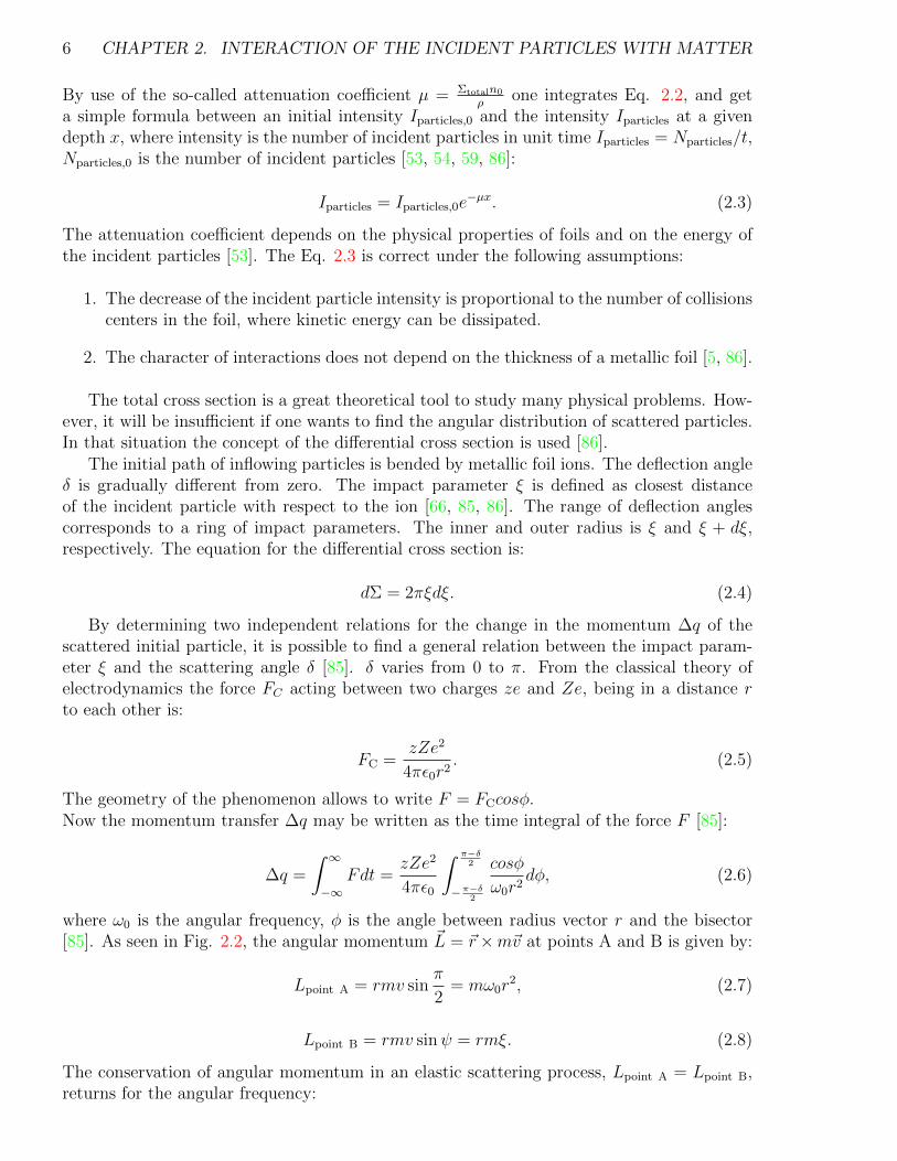
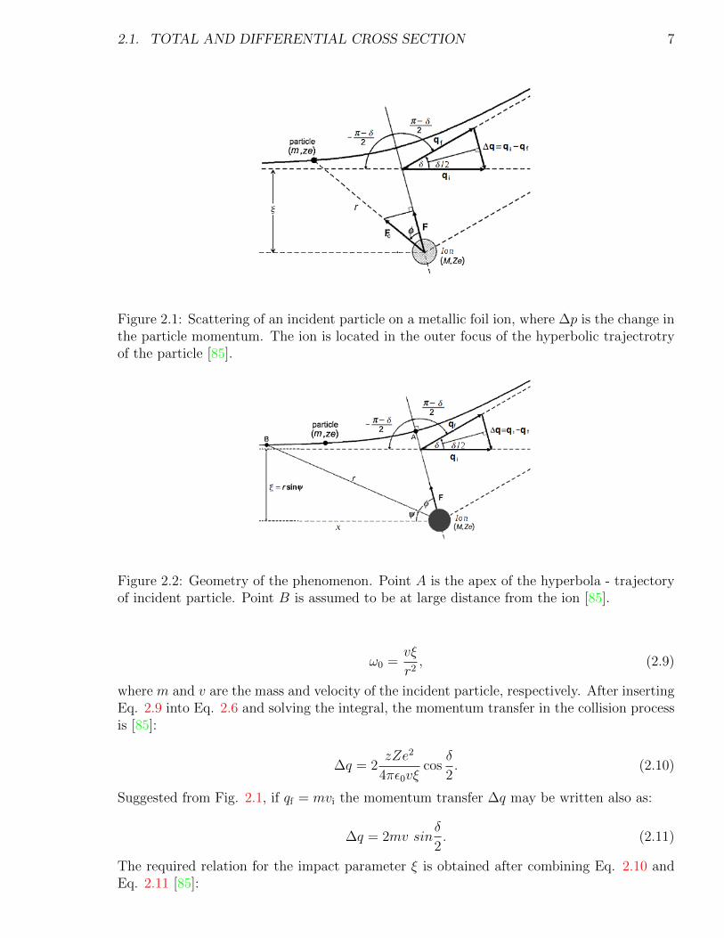
where ω0 is the angular frequency, φ is the angle between radius vector r and the bisector[85]. As seen in Fig. 2.2, the angular momentum ~L = ~r×m~v at points A and B is given by:
Lpoint A = rmv sinπ
2= mω0r
2, (2.7)
Lpoint B = rmv sinψ = rmξ. (2.8)
The conservation of angular momentum in an elastic scattering process, Lpoint A = Lpoint B,returns for the angular frequency:
2.1. TOTAL AND DIFFERENTIAL CROSS SECTION 7
Figure 2.1: Scattering of an incident particle on a metallic foil ion, where ∆p is the change inthe particle momentum. The ion is located in the outer focus of the hyperbolic trajectrotryof the particle [85].
Figure 2.2: Geometry of the phenomenon. Point A is the apex of the hyperbola - trajectoryof incident particle. Point B is assumed to be at large distance from the ion [85].
ω0 =vξ
r2, (2.9)
where m and v are the mass and velocity of the incident particle, respectively. After insertingEq. 2.9 into Eq. 2.6 and solving the integral, the momentum transfer in the collision processis [85]:
∆q = 2zZe2
4πε0vξcos
δ
2. (2.10)
Suggested from Fig. 2.1, if qf = mvi the momentum transfer ∆q may be written also as:
∆q = 2mv sinδ
2. (2.11)
The required relation for the impact parameter ξ is obtained after combining Eq. 2.10 andEq. 2.11 [85]:
8 CHAPTER 2. INTERACTION OF THE INCIDENT PARTICLES WITH MATTER
ξ =zZe2
8πε0EKcot
δ
2, (2.12)
where z and Z are the atomic numbers of a incident particle and a foil ion respectively. EKis the kinetic energy of an incident particle. One can now write the Eq. 2.4 in a differentform:
dΣ = 2πξ
sinδsinδ
∣∣∣∣dξdδ∣∣∣∣ dδ. (2.13)
Calculating dξdδ
and using the solid angle dΩ = 2πsinδ dδ one has:
dΣ
dΩ=
(zZe2
16πε0EK
)21
sin4 δ2
. (2.14)
Equation 2.14 describes the differential cross section for scattered particles. It is calledthe Rutherford formula [85, 86]. The cross section depends on two factors:
1. If the kinetic energy of incident particles increases, then the differential cross sectionwill decrease. Therefore, the incident particles with the lower kinetic energy will havea higher probability to be scattered off by ions of the foil.
2. For a given target foil (Ze) and given incident particle (ze, EK), a large differentialcross section implies a small scattering angle δ.
3. In the process of continuous irradiation of the foil with electrons and/or ions, the degreeof ionization of the foil atoms (see Section 2.2) grow, hence, the degradation processmay be characterized by the increase of the differential cross section.
2.2 Energy loss per unit length by ionization and exci-
tation
Collisions with ions of the metallic foil are caused by incident particles which penetrate thematerial, hence ions can get additional energy. Atoms can be excited or ionized, while theincident particles lose their energies simultaneously [86]. If the energy loss per unit length perion is known, one can calculate the energy loss per unit length of an incident particle, whichtravels through the foil: −dE/dx. It is proved experimentally, that this quantity dependson the type and on the energy of the incident particle and on the physical properties of themetallic foil [5, 86]. The required formula is obtained by use of the principle of conservationof energy and momentum, taking into account also the geometry of the phenomenon. Onlyperpendicular forces act on the incident particle. Forces parallel to the line of flight arecanceled out by the symmetry [66]:
F =zZe2
4πε0r2sinψ, dt =
dx
v, (2.15)
where dx is the path of the incident particle which moves in unit time dt. Now, using thegeometry of the collision process (Fig. 2.2):
ξ
x= tanψ, r =
ξ
sinψ, dx = − ξ
sin2 ψdψ. (2.16)
2.3. INTERACTIONS OF PROTONS WITH MATTER 9
The momentum transfer ∆q of the incident [66] is:
∆q =
∫ ∞−∞
Fdt = − zZe2
4πε0ξv
∫ π
0
sinψdψ. (2.17)
The energy transfered to the metallic foil nuclei is [66]:
∆q2
2M=
1
2M
(zZe2
2πε0ξv
)2
. (2.18)
The energy loss rate per unit length dx is the product of Eq. 2.18 and the number of collisionsin the metallic foil with impact parameter in range ξ to ξ + dξ:
dE
dx= −
∫ ξmax
ξmin
n02πξdξ1
2M
(zZe2
2πε0ξv
)2
. (2.19)
Finally, after integration, one finds:
dE
dx= − n0
πM
(zZe2
2ε0v
)2
ln
(ξmaxξmin
), (2.20)
where M is the mass of an ion of the metallic foil material, v is the velocity of the incidentparticle. The energy loss per unit length depends on:
• the velocity of the incident particle ∼ v−2. The higher the kinetic energy, the lowerloss rate.
• the square of the incident and ion number, z2 and Z2, respectively. It means that ifz increases by a factor of two, the energy loss rate per unit length will increase by afactor of four, hence, Eq. 2.20 is very sensitive for changes of the atomic numbers andionization process.
• the logarithm of ratio of the upper and lower limits of the impact parameter, i.e. its aweak dependency.
The evaluation of ξmax and ξmin will be studied in next subsections, for the protons as incidentparticles. The case of relativistic protons as the incident particles will be considered as well.
2.3 Interactions of protons with matter
The previous subsection discusses the general problem of the energy loss per unit length byan incident particle. According to the experimental data [102] protons lose energy whilepenetrating a target mainly by collisions with electrons. Target atoms are then ionizedadditionally. Therefore the relation 2.20 has to be modified. The mass of the target ion Mis replaced by the mass of an electron me:
dE
dx= − n0
πme
(zZe2
2ε0v
)2
ln
(ξmaxξmin
), (2.21)
This subsection studies the integration limits of the impact parameter, Eq. 2.21 in twocases: non - relativistic and relativistic, respectively.
10 CHAPTER 2. INTERACTION OF THE INCIDENT PARTICLES WITH MATTER
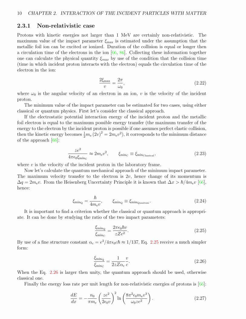
2.3.1 Non-relativistic case
Protons with kinetic energies not larger than 1 MeV are certainly non-relativistic. Themaximum value of the impact parameter ξmax is estimated under the assumption that themetallic foil ion can be excited or ionized. Duration of the collision is equal or longer thena circulation time of the electrons in the ion [66, 86]. Collecting these information togetherone can calculate the physical quantity ξmax by use of the condition that the collision time(time in which incident proton interacts with the electron) equals the circulation time of theelectron in the ion:
2ξmax
v=
2π
ω0
, (2.22)
where ω0 is the angular velocity of an electron in an ion, v is the velocity of the incidentproton.
The minimum value of the impact parameter can be estimated for two cases, using eitherclassical or quantum physics. First let’s consider the classical approach.
If the electrostatic potential interaction energy of the incident proton and the metallicfoil electron is equal to the maximum possible energy transfer (the maximum transfer of theenergy to the electron by the incident proton is possible if one assumes perfect elastic collision,then the kinetic energy becomes 1
2me (2v)2 = 2mev
2), it corresponds to the minimum distanceof the approach [66]:
ze2
4πε0ξminC
≈ 2mev2, ξminC
≡ ξminClassical, (2.23)
where v is the velocity of the incident proton in the laboratory frame.Now let’s calculate the quantum mechanical approach of the minimum impact parameter.
The maximum velocity transfer to the electron is 2v, hence change of its momentum is∆q = 2mev. From the Heisenberg Uncertainty Principle it is known that ∆x > ~/4mev [66],hence:
ξminQ=
~4mev
, ξminQ≡ ξminQuantum
. (2.24)
It is important to find a criterion whether the classical or quantum approach is appropri-ate. It can be done by studying the ratio of the two impact parameters:
ξminQ
ξminC
=2πε0~vzZe2
. (2.25)
By use of a fine structure constant αc = e2/4πε0c~ ≈ 1/137, Eq. 2.25 receive a much simplerform:
ξminQ
ξminC
=1
2zZαc
v
c. (2.26)
When the Eq. 2.26 is larger then unity, the quantum approach should be used, otherwiseclassical one.
Finally the energy loss rate per unit length for non-relativistic energies of protons is [66]:
dE
dx= − n0
πme
(ze2
2ε0v
)2
ln
(8π2ε0mev
3
ω0ze2
). (2.27)
2.3. INTERACTIONS OF PROTONS WITH MATTER 11
The corresponding formula for quantum case is:
dE
dx= − n0
πme
(ze2
2ε0v
)2
ln
(4πmev
2
~ω0
). (2.28)
Equation 2.28 can be rewritten into a more simple and usable form. First step is to replace~ω0 by its relation to the binding energy 1
2~ω0 of the electron in Bohr’s description [66]. The
binding energy is also the ionization potential Ip which should be a properly weighted meanover all states of the electrons in the metallic foil ions Ip that ionization potential has to befound experimentally [66]. In a second step we put all this information together and find:
ln
(2πmev
2
~ω0
)≡ ln
(2mev
2
Ip
), (2.29)
In classical approach the energy loss per unit length depends almost on the same conditionsas in Eq. 2.21, because logarithm yields a relatively small correction only.
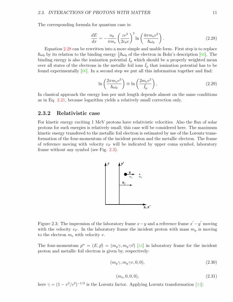
2.3.2 Relativistic case
For kinetic energy exciting 1 MeV protons have relativistic velocities. Also the flux of solarprotons for such energies is relatively small; this case will be considered here. The maximumkinetic energy transfered to the metallic foil electron is estimated by use of the Lorentz trans-formation of the four-momentum of the incident proton and the metallic electron. The frameof reference moving with velocity vF will be indicated by upper coma symbol, laboratoryframe without any symbol (see Fig. 2.3).
Figure 2.3: The impression of the laboratory frame x−y and a reference frame x′−y′ moving
with the velocity vF . In the laboratory frame the incident proton with mass mp is movingto the electron me with velocity v.
The four-momentum pα = (E, ~p) = (mpγ,mpγ~v) [44] in laboratory frame for the incidentproton and metallic foil electron is given by, respectively:
(mpγ,mpγv, 0, 0), (2.30)
(me, 0, 0, 0), (2.31)
here γ = (1− v2/c2)−1/2 is the Lorentz factor. Applying Lorentz transformation [44]:
12 CHAPTER 2. INTERACTION OF THE INCIDENT PARTICLES WITH MATTER
x′ = γF(x− vFt), (2.32)
t′ = γF
(t− vF
c2x), (2.33)
where vF is the velocity of the moving reference frame, vF ||v, one can calculate the four-velocity and the four-momentum in the reference frame of the incident proton and the metallicelectron, respectively [66] one finds:
v′ = γF(v − vF) ⇒ (γmpv)′ = γF(γmpv − γmpvF), (2.34)
v′e = γF(0− vF) ⇒ p′e = −γFmevF. (2.35)
In the center of momentum frame in which the center of mass is at rest (γmpv)′+ p′i = 0 onecan calculate the velocity of the reference frame:
vF =γmpv
me + γmp
. (2.36)
The 0-component of the four-momentum of the electron in the laboratory frame is:
p0 = γ
(meγF +
v2F
c2meγF
). (2.37)
Assuming that γmp me and taking into account Eq. 2.36 it is vF ≈ v and γF ≈ γ, hence:
p0 = γ2me
(1 +
v2
c2
). (2.38)
The total energy transfered to the electron is:
E = γ2mec2
(1 +
v2
c2
). (2.39)
Therefore its kinetic energy is:
EK = E −mec2 = mec
2γ2
(1 +
v2
c2− 1
γ2
). (2.40)
The maximum kinetic energy transferred to the electron by the incident proton is then [66]:
EKmax = 2meγ2v2. (2.41)
Now using Eq. 2.41 it is easy to write the logarithm for the energy loss per unit length Eq.2.20:
ln
(ξmax
ξmin
)≡ ln
(EKmax
Ip
)= ln
(2γ2mev
2
Ip
). (2.42)
The exact formula of the energy loss per unit length of incident proton in the quantum-relativistic description is known as the Bethe-Bloch formula [113]:
− dE
dx=
n0
πme
(ze2
2ε0v
)2 [ln
(2γ2mev
2
Ip
)− 2 ln γ + γ−2 − 1
]. (2.43)
2.4. RECOMBINATION OF ELECTRONS AND PROTONS TO HYDROGEN 13
The second and the third terms are correction factors that are neglected for low velocities ofthe incident particles [113]. The Bethe - Bloch formula depends on:
• the velocity of the incident particle. The increase of that velocity decreases the energyloss per unit length.
• charge z of the incident particle (here proton). With an increase of the charges, theloss per unit length increases too.
2.4 Recombination of electrons and protons to Hydro-
gen
Rausch von Traubenberg and Hahn in 1922 have discovered for the very first time a protonrecombination process [116]; they used thin films as targets. Basic aspects of two-electronAuger recombination of low energy ions at surfaces, originally proposed by Shekhter already in1937, has been described extensively within a probability model by Hagstrum [43]. In 1987,Taute considered variability of Auger recombination rate as a function of an ion velocity.There have been considered small grazing angles [104, 116].
In solids one can distinguish four processes of recombination of incident H+ ions (protons)with electrons to neutral Hydrogen atoms:
1. the Auger process,
2. the resonant process,
3. Oppenheimer-Brinkman-Kramers (OBK) process,
4. Radiative Electron Capture (REC) process.
Since the solar wind consists mainly of low (≤ 100 keV) energetic protons only the firstthree processes will be considered in this thesis. The Auger process dominates the total crosssection [101]. According to Raisbeck and Yiou [87] for protons the REC process dominatesthe recombination only above proton energies of about 300 MeV (for Al foil); therefore thisprocess will be not discussed here.
For each of these recombination processes one can calculate the rate Γ of capture (recom-bination rate) or loss (ionization rate) of an electron. The cross section per atom for eachcharge exchange process is defined by [84]:
Σ =Γ
n0v, (2.44)
where v is the ion speed and n0 is the number density of material ions.
The plan of this section is as follows: first a short introduction to the Hydrogen atomin a classical and quantum approach is made. Next a description of conditions which haveinfluence to the number of free electrons in solids is made. Finally the recombination processesare described.
14 CHAPTER 2. INTERACTION OF THE INCIDENT PARTICLES WITH MATTER
The Hydrogen atom - quasi-classical approach
The classical description of the Hydrogen atom is based on two assumptions:
1. An electron with mass me in an atom orbits with a radius re(n) and velocity ve(n) theproton. n is a number of the shell. The angular momentum is defined as:
meve(n)re(n) = n~, n = 1, 2, 3, .... (2.45)
2. An atom emits a photon of electromagnetic radiation when an electron jumps to lowershell. On the other hand it jumps to higher shell when it absorbs a photon. The energydifference ∆E is proportional to the frequency of the electromagnetic radiation:
∆E = hν. (2.46)
Radius, velocity and energy of an electron at the n’th shell are calculated by use of bothBohr’s assumptions and the balance of the centripetal and Coulomb forces:
re(n) =n2~2
mee2, ve(n) =
e2
n~, E(n) = − 1
n2
mee4
2~2. (2.47)
For n = 1, the minimum radius (the Bohr radius) and the energy (the Bohr energy) for anelectron are:
rBohr =~2
mee2∼= 5.29× 10⁻⁹ cm, EBohr = −mee
4
2~2∼= −13.6 eV. (2.48)
The Hydrogen atom - quantum approach
In quantumm physics the Hamiltonian of the Hydrogen atom and the Schrodinger equationare:
H = − ~2
2me
∇2 + V (r), Hψ(r, θ, φ) = Eψ(r, θ, φ), (2.49)
where V (r) is the potential energy, V (r) = − e2
r. The state function is written in spherical
coordinates as [95, 103]:
ψ(r, θ, φ) =Rn,l(r)
rYl,m(θ, φ), (2.50)
while its angular part is described by spherical harmonics. The radial part fulfills the followingordinary secondary differential equation [95, 103]:
d2Rn,l(r)
dr2+
2me
~2
(En +
e2
r
)− l(l − 1)
r2
Rn,l(r) = 0, l = 0, 1, 2, .... (2.51)
Here l is the orbital quantum number. The energy of an electron at the n’th shell is:
En = − 1
n2
mee4
2~2, (2.52)
2.4. RECOMBINATION OF ELECTRONS AND PROTONS TO HYDROGEN 15
which is the same result obtained from classical approach (see Equation 2.47). The radialpart of the state function is:
Rn,l(r)
r= e−iknrrlL2l+1
n+1 (2knr), (2.53)
where kn =√−2meEn
~2 and L2l+1n+1 (x) is the Laguerre polynomial:
L2l+1n+1 (x) =
d2l+1
dx2l+1
ex
dn+l
dxn+1
(xn+le−x
). (2.54)
A detailed derivation can be found in the standard text books [57, 95, 103].
Number of free electrons in solids
Each solid at given physical conditions (temperature, pressure) has an approximately con-stant number of free electrons. A possibility to change the number is to irradiate the targetby incident particles.
The number of lattice ions per unit volume is:
n0 =NAρ
Mu
, (2.55)
where NA is the Avogadro’s number (6.022× 10²³ mol−1), ρ the density of a given material,Mu is the molar mass, it is 27 g mol−1 for Aluminum and n0 is 6.026× 10²² atoms cm−3.
According to [37] one can estimate a number of free electrons ne per one lattice atom asa function of conductivity σ:
nen0
=
(3
8π
) 12 1
n0
h32
e3
(σl
) 32, (2.56)
Here l is the mean free path. The conductivity which is related to the resistivity σ = 1/%[37]. The resistivity obeys the Matthiessen’s rule (not satisfied for Noble metals: ruthenium,rhodium, palladium, silver, osmium, iridium, platinum and gold) [115]:
%total = %(T ) + %impurities(x) + %crystal imperfections, (2.57)
where x is the concentration of impurities. The first term of this formula is given by theBloch - Gruneisen relation [115]:
%(T ) = %(0) + A
(T
Θ
)∫ ΘT
0
xni
(ex − 1)(1− e−x)dx. (2.58)
Here A is a constant number that depends on a velocity of the electrons at the Fermi surfaceand the Debye radius and a density of electrons in the meta. Θ is the Debye temperature,ni is an integer, where [13, 115]:
• ni = 2 means that resistivity is determined by electron - electron interactions,
• ni = 5 means that resistivity is determined by scattering of electrons by phonons.
16 CHAPTER 2. INTERACTION OF THE INCIDENT PARTICLES WITH MATTER
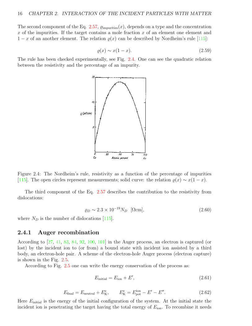
The second component of the Eq. 2.57, %impurities(x), depends on a type and the concentrationx of the impurities. If the target contains a mole fraction x of an element one element and1− x of an another element. The relation %(x) can be described by Nordheim’s rule [115]:
%(x) ∼ x(1− x). (2.59)
The rule has been checked experimentally, see Fig. 2.4. One can see the quadratic relationbetween the resistivity and the percentage of an impurity.
Figure 2.4: The Nordheim’s rule, resistivity as a function of the percentage of impurities[115]. The open circles represent measurements; solid curve: the relation %(x) ∼ x(1− x).
The third component of the Eq. 2.57 describes the contribution to the resistivity fromdislocations:
%D ∼ 2.3× 10⁻¹⁹ND [Ωcm], (2.60)
where ND is the number of dislocations [115].
2.4.1 Auger recombination
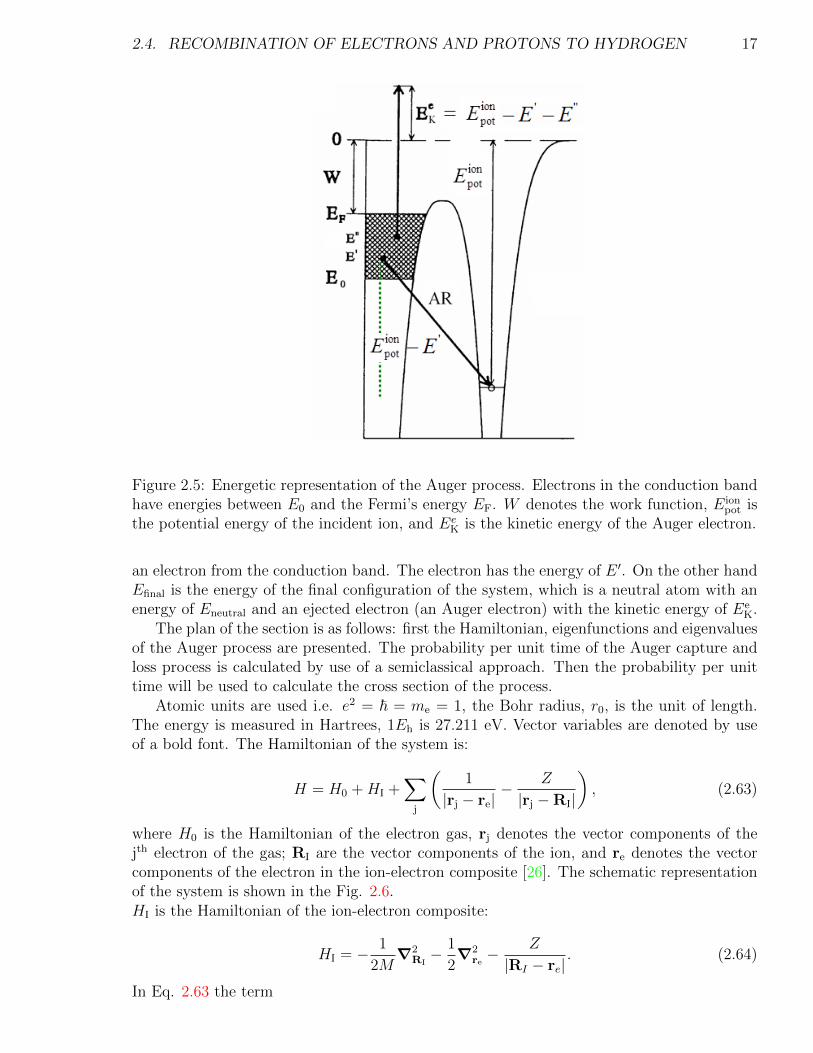
According to [27, 41, 83, 84, 92, 100, 101] in the Auger process, an electron is captured (orlost) by the incident ion to (or from) a bound state with incident ion assisted by a thirdbody, an electron-hole pair. A scheme of the electron-hole Auger process (electron capture)is shown in the Fig. 2.5.
According to Fig. 2.5 one can write the energy conservation of the process as:
Einitial = Eion + E ′, (2.61)
Efinal = Eneutral + EeK, Ee
K = Eionpot − E ′ − E ′′. (2.62)
Here Einitial is the energy of the initial configuration of the system. At the initial state theincident ion is penetrating the target having the total energy of Eion. To recombine it needs
2.4. RECOMBINATION OF ELECTRONS AND PROTONS TO HYDROGEN 17
Figure 2.5: Energetic representation of the Auger process. Electrons in the conduction bandhave energies between E0 and the Fermi’s energy EF. W denotes the work function, Eion
pot isthe potential energy of the incident ion, and Ee
K is the kinetic energy of the Auger electron.
an electron from the conduction band. The electron has the energy of E ′. On the other handEfinal is the energy of the final configuration of the system, which is a neutral atom with anenergy of Eneutral and an ejected electron (an Auger electron) with the kinetic energy of Ee
K.The plan of the section is as follows: first the Hamiltonian, eigenfunctions and eigenvalues
of the Auger process are presented. The probability per unit time of the Auger capture andloss process is calculated by use of a semiclassical approach. Then the probability per unittime will be used to calculate the cross section of the process.
Atomic units are used i.e. e2 = ~ = me = 1, the Bohr radius, r0, is the unit of length.The energy is measured in Hartrees, 1Eh is 27.211 eV. Vector variables are denoted by useof a bold font. The Hamiltonian of the system is:
H = H0 +HI +∑
j
(1
|rj − re|− Z
|rj −RI|
), (2.63)
where H0 is the Hamiltonian of the electron gas, rj denotes the vector components of thejth electron of the gas; RI are the vector components of the ion, and re denotes the vectorcomponents of the electron in the ion-electron composite [26]. The schematic representationof the system is shown in the Fig. 2.6.HI is the Hamiltonian of the ion-electron composite:
HI = − 1
2M∇2
RI− 1
2∇2
re− Z
|RI − re|. (2.64)
In Eq. 2.63 the term
18 CHAPTER 2. INTERACTION OF THE INCIDENT PARTICLES WITH MATTER
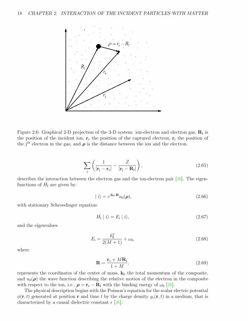
Figure 2.6: Graphical 2-D projection of the 3-D system: ion-electron and electron gas, RI isthe position of the incident ion, re the position of the captured electron, rj the position ofthe jth electron in the gas, and ρ is the distance between the ion and the electron.
∑j
(1
|rj − re|− Z
|rj −RI|
), (2.65)
describes the interaction between the electron gas and the ion-electron pair [26]. The eigen-functions of HI are given by:
| i〉 = eik0·Ru0(ρ), (2.66)
with stationary Schroedinger equation:
HI | i〉 = Ei | i〉, (2.67)
and the eigenvalues
Ei =k2
0
2(M + 1)+ ω0, (2.68)
where
R =re +MRI
1 +M, (2.69)
represents the coordinates of the center of mass, k0 the total momentum of the composite,and u0(ρ) the wave function describing the relative motion of the electron in the compositewith respect to the ion, i.e., ρ = re −RI with the binding energy of ω0 [26].
The physical description begins with the Poisson’s equation for the scalar electric potentialφ(r, t) generated at position r and time t by the charge density %c(r, t) in a medium, that ischaracterized by a causal dielectric constant ε [26]:
2.4. RECOMBINATION OF ELECTRONS AND PROTONS TO HYDROGEN 19
ε∇2φ = −4π%c(r, t). (2.70)
An incident particle with charge Z may be considered to give rise to a charge density%c(r, t) = Zδ(r− vt) [26]. To write the equation in the momentum space, one has to use theFourier transformation:
f(q, ω) =
∫d3q
(2π)3
∫ ∞−∞
dω e−i(q·r−ωt)fr,t, (2.71)
where q is the momentum and ω the energy. Thus the density is %q,ω = 2πZδ(ω−q · v). Byuse of Eqs. 2.70 and 2.71 one can calculate the scalar potential:
φq,ω =4π%c(q, ω)
q2ε(q, ω). (2.72)
An incident particle moving through the target with velocity v induces an electric field,whose scalar potential is given by [27]:
φindq,ω =
8π2Z
q2δ(ω − q · v)
(1
ε(q, ω)− 1
). (2.73)
When an incident particle is passing through the matter, the induced potential aroundthe moving ion deviates from the spherical symmetry. For a charge at rest this potentialis spherically symmetric, but as its velocity increases the potential loses this symmetry. Astrong modification of this type should create an important effect to the state of the electronwhich is bound to the ion [41]. Additionally, at the end of the subsection this effect willbe presented by use of the wave function u0(ρ) which describes the relative motion of theelectron in the ion-electron composite .
The rate of energy loss per unit time of the incident particle dEdt
is obtained from the
induced electric field Eind = −∇φind [26]:
dE
dt= −Zv · Eind(r, t). (2.74)
According to [26] one can write the energy loss as:
dE
dt=
∫d3q
(2π)3
∫ ∞0
dω
2π2ωZIm(−φind
q,ω) (2.75)
It is taken only the imaginary part of the potential, i.e. imaginary part of the dielectric
function: Im(− 1ε(q,ω)
). According to Jackson [49] the imaginary part of ε represents the
energy dissipation of an electromagnetic wave in the medium. If Im(ε) < 0 then energy istransfered from the media to the wave. dE
dtcan also be written in much more suitable form
[26]:
dE
dt=
∫dx ωΓ(q, ω),
∫dx ≡
∫d3q
(2π)3
∫ ∞0
dω
2π, (2.76)
where Γ(q, ω) is the probability per unit time that the initial ion loses energy ω and mo-mentum q [26] (q and ω represent the momentum and energy transferred to the solid by anincident particle [92]):
20 CHAPTER 2. INTERACTION OF THE INCIDENT PARTICLES WITH MATTER
Γ(q, ω) = 2ZIm(−φindq,ω) =
16π2Z2
q2Im
(− 1
ε(q, ω)
)δ(ω − q · v). (2.77)
Note that the energy loss per unit length dx can be written immediately by use of the Eq.2.76:
dE
dx=
1
v
∫dx ωΓ(q, ω). (2.78)
To adopt the result of Eq. 2.77 to the Auger process one has to consider a few corrections:
1. When an incident particle captures an electron that lies inside the Fermi sphere |k + v |< kF , where k is the momentum of the electron, kF is the Fermi’s wave number.On the other hand when the particle loses an electron, an electron-hole pair is created,and | k + v |> kF . One can clearly imagine this situation considering the Fig. 2.5.Thus the first multiplication correction factor to Eq. 2.77 is:
Θ(±kF∓ | k + v |), (2.79)
where Θ(x) is the step function, Θ(x) = 1 when x ≥ 0, and Θ(x) = 0 when x < 0.Upper signs (+/−) denote capture of an electron by incident ion, while lower signs(−/+) loss of the electron.
2. If one looks carefully to the energy conservation of the process, Eqs. 2.61 and 2.62, itis obvious that in each single process the energy of the ejected Auger electron couldbe different, it mainly depends on the energy of the incident ions. Also the energy ofthe bound to the incident ion-electron could be different because it is inside the Fermisphere having an energy waring in the range of E0 to EF.
The recombination will proceed more rapidly if the coupling between the initial andfinal states is stronger. This coupling term is traditionally called the matrix element :〈f | A | i〉. The matrix element can be placed in the form of an integral, wherethe interaction which causes the process is expressed as an operator A which actson the initial state wavefunction. The recombination probability is proportional tothe square of the integral. This kind of approach using the wavefunctions is of thesame general form as that used to find the expectation value of any physical variablein quantum mechanics [47]. Here the initial eigenstate |i〉 is described by use of theu0(ρ) wave function; final eigenstate 〈f | by use of OPW (Orthogonal Plane Wave)function | kOPW〉 =| eik·ρ〉 − 〈u0(ρ) | eik·ρ〉 | u0(ρ)〉 [26]. An OPW is defined as a planewave which has been made orthogonal to Bloch waves by use of the Schmidt process[1, 16, 46]. OPW describes the state of an electron in the conduction band in solids[26]; the method was proposed by Herring in 1940 [46]. In the literature one can findalso the method proposed by Wigner and Seitz [108] which gives good results for lowerstates of the valence electron band of a metal, but the extension of this method tostates of higher energy becomes rapidly more unreliable as the energy increases [26].Here A is an operator for the physical interaction which couples the initial and finalstates of the system; A is here e±k·ρ. Thus the second multiplication correction factoris:
| 〈kOPW | e±k·ρ | u0(ρ)〉 |2 . (2.80)
2.4. RECOMBINATION OF ELECTRONS AND PROTONS TO HYDROGEN 21
Upper sign (+) denotes capture of an electron by the incident ion, while lower sign (−)loss of the electron.
3. Also one has to modify the δ function. The correction takes into a account capturedor an ejected electron [26]:
δ(ω − q · v∓ k2
2± ω0) (2.81)
Upper signs (−/+) denotes capture of an electron by the incident ion, while lower signs(+/−) loss of the electron.
Thus the probability per unit time of electron capture or loss in the Auger process is[27, 83, 92, 100, 101]:
ΓC,LA =
∫d3q
(2π)3
∫ ∞0
dω
2π
∫d3k
(2π)3Θ(±kF∓ | k + v |) (2.82)
16π2Z2
q2Im
(− 1
ε(q, ω)
)δ(ω − q · v∓ k2
2± ω0)
| 〈kOPW | e±k·ρ | u0(ρ)〉 |2 .
By use both Eqs. 2.44 and 2.82 one can easily calculate the cross section of the Augerprocess, both for losing and capturing of an electron.
According to [26, 41] the bound state wave function (the wave function describing therelative motion of the electron in the composite with respect to the ion) is assumed to be ofthe form:
u0(ρ) =
(a3
π
) 12
exp(−aρ). (2.83)
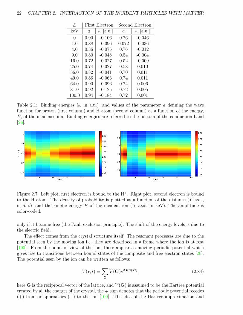
Guinea et al. [41] have calculated the wave functions and the binding energies, ω, of the firstand second electron bound to H. Results are presented in the Table 2.1.
One can calculate the probability amplitude by use of well-known formula Π ∼| u0(ρ) |2.Here Π predicts the position where the bound (to the incident ion) state is most probable.Results are presented in Fig. 2.7 where the incident particle is a proton. The left plot showsthe situation where the first electron is bound to the proton; while in the right plot thesecond electron is bound to the H atom. The amplitude | u0(ρ) |2 is plotted as a function ofthe distance (Y axis, in a.u.) from the incident proton or H atom and of the energy of theincident proton or H atom (X axis, in keV).
It is obvious that the smaller the distance to the incident proton or H atom, the higheris the probability of a recombination event. While the kinetic energy energy of the incidentH is much smaller than for proton.
2.4.2 Resonant recombination
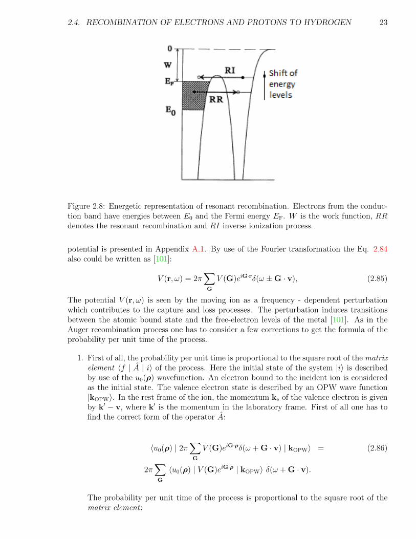
The incident ion is recombined with an electron which is tunneled to the metastable state[43], see Fig 2.8. The inverse process is also possible. An electron which is in a metastablestate with respect to the metallic ion can populate one of the free electron states of the metal
22 CHAPTER 2. INTERACTION OF THE INCIDENT PARTICLES WITH MATTER
E First Electron Second ElectronkeV a ω [a.u.] a ω [a.u.]
0 0.90 -0.106 0.76 -0.0461.0 0.88 -0.096 0.072 -0.0364.0 0.86 -0.075 0.76 -0.0129.0 0.80 -0.048 0.54 -0.00416.0 0.72 -0.027 0.52 -0.00925.0 0.74 -0.027 0.58 0.01036.0 0.82 -0.041 0.70 0.01149.0 0.86 -0.063 0.74 0.01164.0 0.90 -0.096 0.74 0.00681.0 0.92 -0.125 0.72 0.005100.0 0.94 -0.184 0.72 0.001
Table 2.1: Binding energies (ω in a.u.) and values of the parameter a defining the wavefunction for proton (first column) and H atom (second column) as a function of the energy,E, of the incidence ion. Binding energies are referred to the bottom of the conduction band[26].
Figure 2.7: Left plot, first electron is bound to the H+. Right plot, second electron is boundto the H atom. The density of probability is plotted as a function of the distance (Y axis,in a.u.) and the kinetic energy E of the incident ion (X axis, in keV). The amplitude iscolor-coded.
only if it become free (the Pauli exclusion principle). The shift of the energy levels is due tothe electric field.
The effect comes from the crystal structure itself. The resonant processes are due to thepotential seen by the moving ion i.e. they are described in a frame where the ion is at rest[100]. From the point of view of the ion, there appears a moving periodic potential whichgives rise to transitions between bound states of the composite and free electron states [26].The potential seen by the ion can be written as follows:
V (r, t) =∑G
V (G)eiG(r∓vt), (2.84)
here G is the reciprocal vector of the lattice, and V (G) is assumed to be the Hartree potentialcreated by all the charges of the crystal, the ∓ sign denotes that the periodic potential recedes(+) from or approaches (−) to the ion [100]. The idea of the Hartree approximation and
2.4. RECOMBINATION OF ELECTRONS AND PROTONS TO HYDROGEN 23
Figure 2.8: Energetic representation of resonant recombination. Electrons from the conduc-tion band have energies between E0 and the Fermi energy EF. W is the work function, RRdenotes the resonant recombination and RI inverse ionization process.
potential is presented in Appendix A.1. By use of the Fourier transformation the Eq. 2.84also could be written as [101]:
V (r, ω) = 2π∑G
V (G)eiG·rδ(ω ±G · v), (2.85)
The potential V (r, ω) is seen by the moving ion as a frequency - dependent perturbationwhich contributes to the capture and loss processes. The perturbation induces transitionsbetween the atomic bound state and the free-electron levels of the metal [101]. As in theAuger recombination process one has to consider a few corrections to get the formula of theprobability per unit time of the process.
1. First of all, the probability per unit time is proportional to the square root of the matrixelement 〈f | A | i〉 of the process. Here the initial state of the system |i〉 is describedby use of the u0(ρ) wavefunction. An electron bound to the incident ion is consideredas the initial state. The valence electron state is described by an OPW wave function|kOPW〉. In the rest frame of the ion, the momentum ke of the valence electron is givenby k′ − v, where k′ is the momentum in the laboratory frame. First of all one has tofind the correct form of the operator A:
〈u0(ρ) | 2π∑G
V (G)eiG·ρδ(ω + G · v) | kOPW〉 = (2.86)
2π∑G
〈u0(ρ) | V (G)eiG·ρ | kOPW〉 δ(ω + G · v).
The probability per unit time of the process is proportional to the square root of thematrix element :
24 CHAPTER 2. INTERACTION OF THE INCIDENT PARTICLES WITH MATTER
ΓLR ∼ 2π
∑G
| V (G) |2| 〈u0(ρ) | eiG·ρ | kOPW〉 |2 δ(ω + G · v), (2.87)
The matrix element describe the electron loss only.
2. The δ function in Eq. 2.87 has to be modified. The correction should take into accountwhether an electron is captured or ejected [27]:
δ(ω − 1
2k2
e ∓G · v) (2.88)
Upper sign (−) denotes the capture of an electron by the incident ion, while lower sign(+) corresponds to the loss of an electron.
3. When an incident particle loses an electron, an electron-hole pair is created, thus |ke + v |> kF. On the other hand, when an incident particle captures an electron it liesinside the Fermi sphere, | ke + v |≤ kF. As in the Auger recombination process one hasto use the Θ(x) step function:
Θ(±kF∓ | ke + v |), (2.89)
Upper signs (+/−) denote capture of an electron by incident ion, while lower signs(−/+) loss of the electron.
Collecting all these information together one can write the probability per unit time ofthe resonant recombination process as [26, 27, 84, 92, 100, 101]:
ΓC,LR = 2π
∫d3k
(2π)3Θ(±kF∓ | ke + v |) δ(ω0 −
1
2k2
e ∓G · v) (2.90)∑G
| V (G) |2| 〈u0(ρ) | eiG·ρ | kOPW〉 |2,
The cross section of this process as well as a comparison with other recombination pro-cesses is presented in the Section 2.4.4.
2.4.3 Oppenheimer - Brinkman - Kramers (OBK) Process
The OBK process is a capture process, where an inner or outer shell electron of a targetatom is transferred to the moving ion [100]. In the literature one can find a lot of physicalapproaches [4, 12, 15, 20, 24, 25, 31, 34, 35, 60, 63, 79]. Different results may be obtaineddepending on the approximation applied to the wave functions and the energy levels involvedin the process [27].
This thesis presents one of them, the author’s modification of so-called model-potentialOBK approximation (MPOBK), the 1s-1s capture. The modification assumes that the massof the incident ion is much lower then the mass of the target’s atom. That is exact thesituation when the metal sample is bombarded by protons. The transition electron caughtby the incident proton is considered as the active electron. The other electrons are consideredto be the passive ones [27]. In the OBK process the outer-shell electrons of the metal ions
2.4. RECOMBINATION OF ELECTRONS AND PROTONS TO HYDROGEN 25
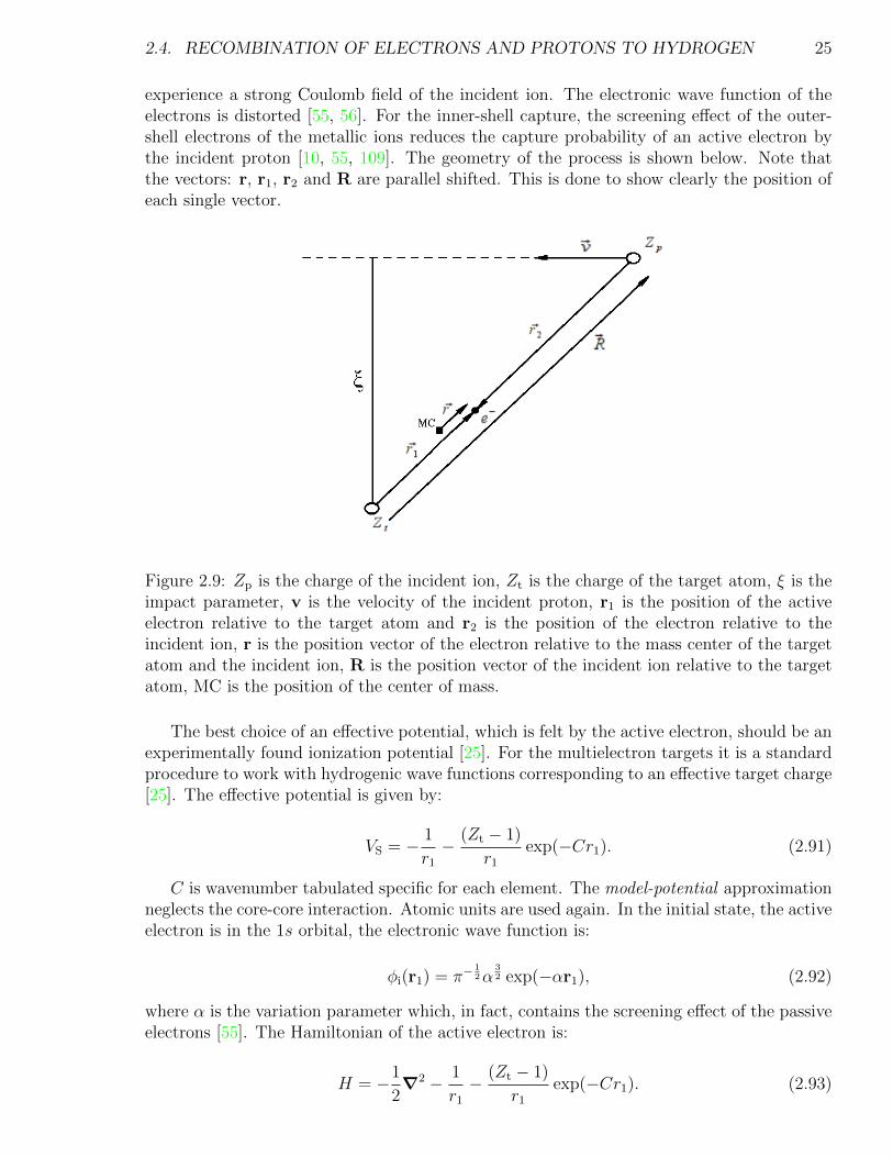
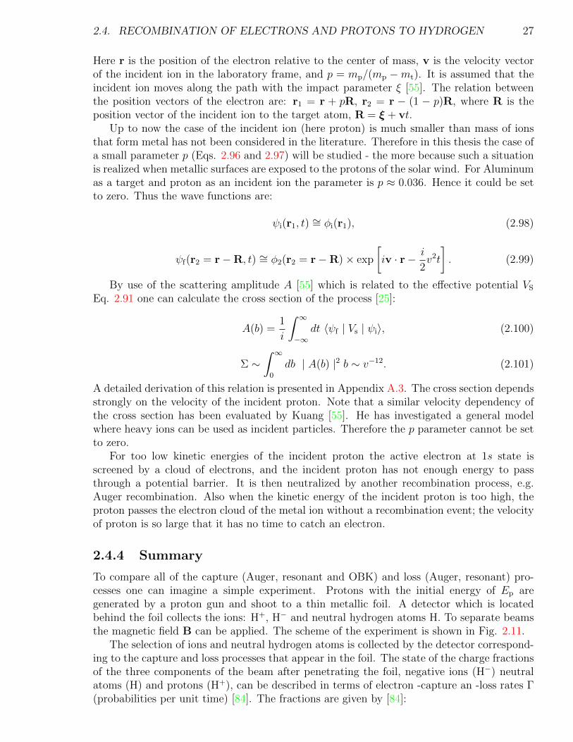
experience a strong Coulomb field of the incident ion. The electronic wave function of theelectrons is distorted [55, 56]. For the inner-shell capture, the screening effect of the outer-shell electrons of the metallic ions reduces the capture probability of an active electron bythe incident proton [10, 55, 109]. The geometry of the process is shown below. Note thatthe vectors: r, r1, r2 and R are parallel shifted. This is done to show clearly the position ofeach single vector.
Figure 2.9: Zp is the charge of the incident ion, Zt is the charge of the target atom, ξ is theimpact parameter, v is the velocity of the incident proton, r1 is the position of the activeelectron relative to the target atom and r2 is the position of the electron relative to theincident ion, r is the position vector of the electron relative to the mass center of the targetatom and the incident ion, R is the position vector of the incident ion relative to the targetatom, MC is the position of the center of mass.
The best choice of an effective potential, which is felt by the active electron, should be anexperimentally found ionization potential [25]. For the multielectron targets it is a standardprocedure to work with hydrogenic wave functions corresponding to an effective target charge[25]. The effective potential is given by:
VS = − 1
r1
− (Zt − 1)
r1
exp(−Cr1). (2.91)
C is wavenumber tabulated specific for each element. The model-potential approximationneglects the core-core interaction. Atomic units are used again. In the initial state, the activeelectron is in the 1s orbital, the electronic wave function is:
φi(r1) = π−12α
32 exp(−αr1), (2.92)
where α is the variation parameter which, in fact, contains the screening effect of the passiveelectrons [55]. The Hamiltonian of the active electron is:
H = −1
2∇2 − 1
r1
− (Zt − 1)
r1
exp(−Cr1). (2.93)
26 CHAPTER 2. INTERACTION OF THE INCIDENT PARTICLES WITH MATTER
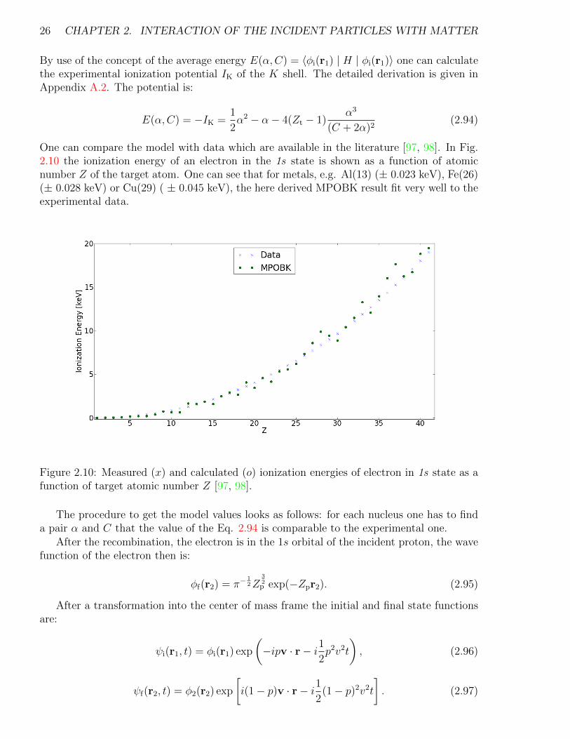
By use of the concept of the average energy E(α,C) = 〈φi(r1) | H | φi(r1)〉 one can calculatethe experimental ionization potential IK of the K shell. The detailed derivation is given inAppendix A.2. The potential is:
E(α,C) = −IK =1
2α2 − α− 4(Zt − 1)
α3
(C + 2α)2(2.94)
One can compare the model with data which are available in the literature [97, 98]. In Fig.2.10 the ionization energy of an electron in the 1s state is shown as a function of atomicnumber Z of the target atom. One can see that for metals, e.g. Al(13) (± 0.023 keV), Fe(26)(± 0.028 keV) or Cu(29) ( ± 0.045 keV), the here derived MPOBK result fit very well to theexperimental data.
Figure 2.10: Measured (x) and calculated (o) ionization energies of electron in 1s state as afunction of target atomic number Z [97, 98].
The procedure to get the model values looks as follows: for each nucleus one has to finda pair α and C that the value of the Eq. 2.94 is comparable to the experimental one.
After the recombination, the electron is in the 1s orbital of the incident proton, the wavefunction of the electron then is:
φf(r2) = π−12Z
32p exp(−Zpr2). (2.95)
After a transformation into the center of mass frame the initial and final state functionsare:
ψi(r1, t) = φi(r1) exp
(−ipv · r− i1
2p2v2t
), (2.96)
ψf(r2, t) = φ2(r2) exp
[i(1− p)v · r− i1
2(1− p)2v2t
]. (2.97)
2.4. RECOMBINATION OF ELECTRONS AND PROTONS TO HYDROGEN 27
Here r is the position of the electron relative to the center of mass, v is the velocity vectorof the incident ion in the laboratory frame, and p = mp/(mp −mt). It is assumed that theincident ion moves along the path with the impact parameter ξ [55]. The relation betweenthe position vectors of the electron are: r1 = r + pR, r2 = r − (1 − p)R, where R is theposition vector of the incident ion to the target atom, R = ξ + vt.
Up to now the case of the incident ion (here proton) is much smaller than mass of ionsthat form metal has not been considered in the literature. Therefore in this thesis the case ofa small parameter p (Eqs. 2.96 and 2.97) will be studied - the more because such a situationis realized when metallic surfaces are exposed to the protons of the solar wind. For Aluminumas a target and proton as an incident ion the parameter is p ≈ 0.036. Hence it could be setto zero. Thus the wave functions are:
ψi(r1, t) ∼= φi(r1), (2.98)
ψf(r2 = r−R, t) ∼= φ2(r2 = r−R)× exp
[iv · r− i
2v2t
]. (2.99)
By use of the scattering amplitude A [55] which is related to the effective potential VS
Eq. 2.91 one can calculate the cross section of the process [25]:
A(b) =1
i
∫ ∞−∞
dt 〈ψf | Vs | ψi〉, (2.100)
Σ ∼∫ ∞
0
db | A(b) |2 b ∼ v−12. (2.101)
A detailed derivation of this relation is presented in Appendix A.3. The cross section dependsstrongly on the velocity of the incident proton. Note that a similar velocity dependency ofthe cross section has been evaluated by Kuang [55]. He has investigated a general modelwhere heavy ions can be used as incident particles. Therefore the p parameter cannot be setto zero.
For too low kinetic energies of the incident proton the active electron at 1s state isscreened by a cloud of electrons, and the incident proton has not enough energy to passthrough a potential barrier. It is then neutralized by another recombination process, e.g.Auger recombination. Also when the kinetic energy of the incident proton is too high, theproton passes the electron cloud of the metal ion without a recombination event; the velocityof proton is so large that it has no time to catch an electron.
2.4.4 Summary
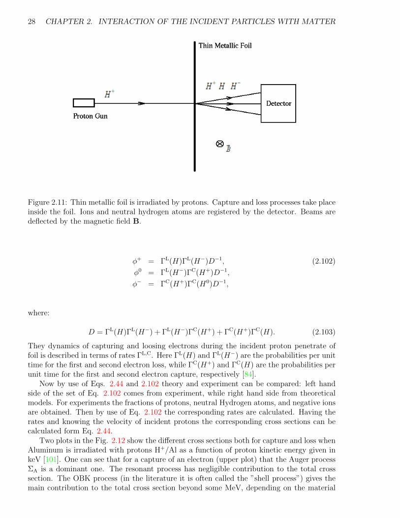
To compare all of the capture (Auger, resonant and OBK) and loss (Auger, resonant) pro-cesses one can imagine a simple experiment. Protons with the initial energy of Ep aregenerated by a proton gun and shoot to a thin metallic foil. A detector which is locatedbehind the foil collects the ions: H+, H− and neutral hydrogen atoms H. To separate beamsthe magnetic field B can be applied. The scheme of the experiment is shown in Fig. 2.11.
The selection of ions and neutral hydrogen atoms is collected by the detector correspond-ing to the capture and loss processes that appear in the foil. The state of the charge fractionsof the three components of the beam after penetrating the foil, negative ions (H−) neutralatoms (H) and protons (H+), can be described in terms of electron -capture an -loss rates Γ(probabilities per unit time) [84]. The fractions are given by [84]:
28 CHAPTER 2. INTERACTION OF THE INCIDENT PARTICLES WITH MATTER
Figure 2.11: Thin metallic foil is irradiated by protons. Capture and loss processes take placeinside the foil. Ions and neutral hydrogen atoms are registered by the detector. Beams aredeflected by the magnetic field B.
φ+ = ΓL(H)ΓL(H−)D−1, (2.102)
φ0 = ΓL(H−)ΓC(H+)D−1,
φ− = ΓC(H+)ΓC(H0)D−1,
where:
D = ΓL(H)ΓL(H−) + ΓL(H−)ΓC(H+) + ΓC(H+)ΓC(H). (2.103)
They dynamics of capturing and loosing electrons during the incident proton penetrate offoil is described in terms of rates ΓL,C. Here ΓL(H) and ΓL(H−) are the probabilities per unittime for the first and second electron loss, while ΓC(H+) and ΓC(H) are the probabilities perunit time for the first and second electron capture, respectively [84].
Now by use of Eqs. 2.44 and 2.102 theory and experiment can be compared: left handside of the set of Eq. 2.102 comes from experiment, while right hand side from theoreticalmodels. For experiments the fractions of protons, neutral Hydrogen atoms, and negative ionsare obtained. Then by use of Eq. 2.102 the corresponding rates are calculated. Having therates and knowing the velocity of incident protons the corresponding cross sections can becalculated form Eq. 2.44.
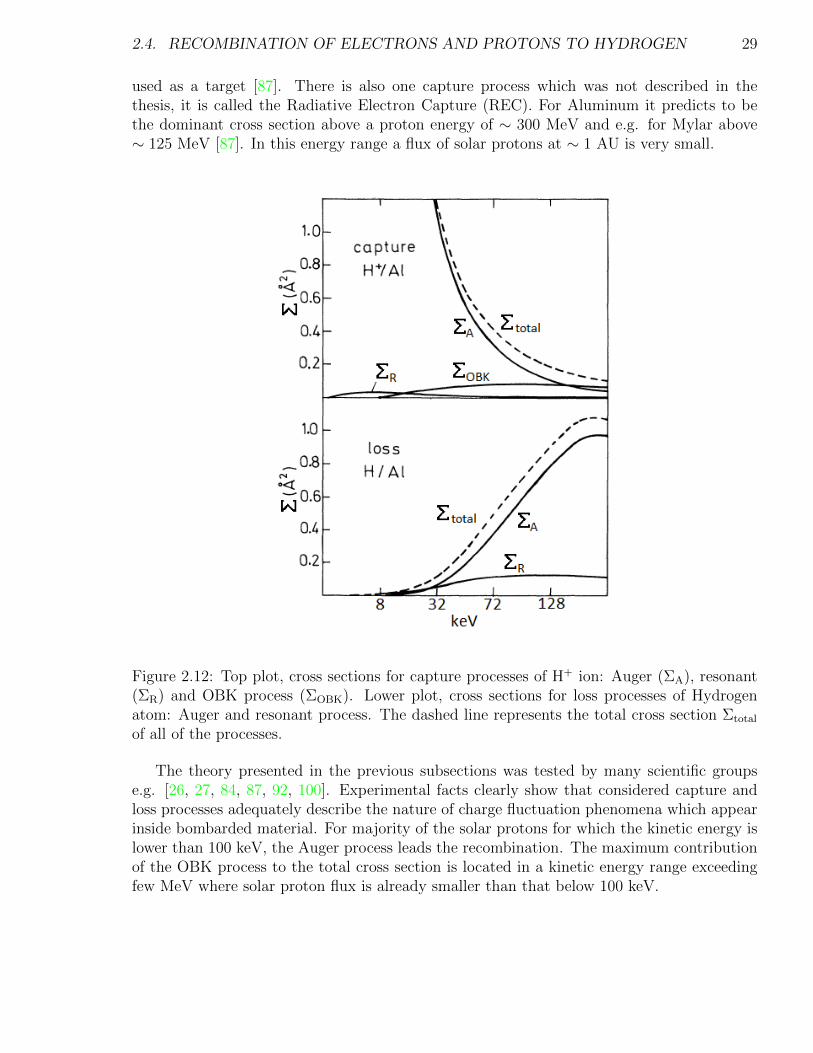
Two plots in the Fig. 2.12 show the different cross sections both for capture and loss whenAluminum is irradiated with protons H+/Al as a function of proton kinetic energy given inkeV [101]. One can see that for a capture of an electron (upper plot) that the Auger processΣA is a dominant one. The resonant process has negligible contribution to the total crosssection. The OBK process (in the literature it is often called the ”shell process”) gives themain contribution to the total cross section beyond some MeV, depending on the material
2.4. RECOMBINATION OF ELECTRONS AND PROTONS TO HYDROGEN 29
used as a target [87]. There is also one capture process which was not described in thethesis, it is called the Radiative Electron Capture (REC). For Aluminum it predicts to bethe dominant cross section above a proton energy of ∼ 300 MeV and e.g. for Mylar above∼ 125 MeV [87]. In this energy range a flux of solar protons at ∼ 1 AU is very small.
Figure 2.12: Top plot, cross sections for capture processes of H+ ion: Auger (ΣA), resonant(ΣR) and OBK process (ΣOBK). Lower plot, cross sections for loss processes of Hydrogenatom: Auger and resonant process. The dashed line represents the total cross section Σtotal
of all of the processes.
The theory presented in the previous subsections was tested by many scientific groupse.g. [26, 27, 84, 87, 92, 100]. Experimental facts clearly show that considered capture andloss processes adequately describe the nature of charge fluctuation phenomena which appearinside bombarded material. For majority of the solar protons for which the kinetic energy islower than 100 keV, the Auger process leads the recombination. The maximum contributionof the OBK process to the total cross section is located in a kinetic energy range exceedingfew MeV where solar proton flux is already smaller than that below 100 keV.

30 CHAPTER 2. INTERACTION OF THE INCIDENT PARTICLES WITH MATTER
Chapter 3
Degradation of materials under spaceconditions
3.1 An overview of degradation processes
3.1.1 Positive electric charging of foils due to irradiation
The surface of the sail-craft will lose electrons and become positively charged by ionization.This can be caused by the photoelectric effect, by Compton scattering and/or by electron -positron pair production when high energy photons hit metallic surfaces [54]. For instanceelectrons may be ejected from the surface by the Auger process (see Section 2.4.1). Partof the electron flux will escape from the sail-craft, another part will be attracted back bythe positively charged sail and therefore partially neutralize it, and third part will producean electron cloud near the surface of the sail which will screen the electric field [54]. Also,electrons from solar wind can partially neutralize the positively charged sail.
During the sail mission total surface charge density can be written as:
∆Qs = e
(dNi
dt− dNr
dt
)∆t, (3.1)
where dNi/dt is the number of sail atoms ionized per second and square meter, dNr/dt isthe number of sail ions recombined per second and square meter, ∆t is the operation timeof the sail mission [54]. Now one can determine the rate of ionization. It is shown e.g. byKazerashvili and Matloff [54] that only a small fraction X% of sail atoms are ionized. X hasto be determined experimentally. In order to estimate the recombination rate of sail atomsper unit area, first one has to calculate the number recombined sail ions per mass. In kg thisis [54]:
NA
A10−3· X
100, (3.2)
where NA is Avogadro’s number and A is the mass number. Multiplying this number by thesail material density ρSail and the thickness of the sail Ls (see Fig. 3.1 [54]) one obtains thenumber of recombined sail ions per unit area:
NAρSailLs
A10−3· X
100. (3.3)
31
32 CHAPTER 3. DEGRADATION OF MATERIALS UNDER SPACE CONDITIONS
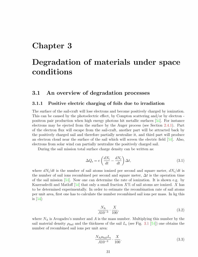
Figure 3.1: Schematic representation how solar wind electrons (black circles) bombard metalions (white circles), of a sail of thickness L [54].
The flux of incident electrons is ne × ve, where ne is the number density and ve the velocityof the incident electrons, respectively. Hence the recombination rate per unit time and areais:
dNr
dt= neve
NAρSailLs
A · 10−3
X
100ΣRR (3.4)
where ΣRR is the total cross section of radiative recombination processes. The cross sectiondecreases with increasing electron energy, as the Bethe-Bloch-equation for the interaction ofelectrons with metal surfaces proves [66]. The recombination rate increases with:
• number density of incident electrons,
• velocity of incident electrons,
• thickness and density of the metallic foil,
• the total cross section of radiative recombination.
On the other hand it decreases with mass number of metallic foil. A charged sail cancause a failure of the electrical equipment mounted in the sail-craft. Charged foils can causealso distortions in a trajectory of the sail-craft, since solar ions are screened by the foil andan additional pushing force may act. Therefore sophisticated methods have to be developedto discharge the sail.
3.1.2 Sputtering - removal of the metallic foil ions by the incidentparticles
Sputtering is defined as removal of material atoms by incident particles: neutral atoms,neutrons, protons or electrons. The sputtering is a well investigated subject, there existmany reviews [11, 17, 51, 73, 74, 99]. Sputtering as a physical process has many usefulapplications:
3.1. AN OVERVIEW OF DEGRADATION PROCESSES 33
• the production of atomically clean surfaces in vacuum,
• analysis of surfaces,
• the production of the thin films.
The production of atomically clean surfaces was studied by Fransworth et al. [30]. Theyhave described, how impurities are removed from surfaces. The bombardment of surfaces ofneutral or charge particles has, however, some unwanted side effects: it damages the surfaces.In this thesis it will be considered only the second point: the analysis of the surfaces andtheir damages.
Methods to analyze materials by sputtering was studied e.g. by Liebl and Herzog [62].The idea is to sputter a target, and the fraction of particles that leaves the material as ions isaccelerated and analyzed in a mass spectrometer. This technique is known as the secondaryion mass spectrometry, the SIMS [74]. The idea is to measure the charged/neutral ratio ofthe sputtered ions, which depends on the state of the surface and can vary from on element toanother. The SIMS method can provide useful information about the physical properties ofthe metallic foil [74]. Castaing and Slodzian [19] used the secondary ion technique for spatialsurface analysis. Abdullayeva el al. [2] have used secondary ions from sputtered surfaces toproduce negative ions for particular applications [74].
An appropriate theory of sputtering was developed e.g. by Sigmund in 1969 [99]. Sig-mund’s description is based on the collision processes, Boltzmann’s equations and generaltransport theory. Sputtering takes place when the incident atoms that sputter off surfaceions have a larger kinetic energy then the surface binding energy of the metal ions. A collisioncascade can be initiated when the incident particle energy E is sufficient to transfer an energygreater than the displacement energy of a lattice atom. Sigmund considered the amount ofenergy per unit length F (x,E, κ) that is transferred to the lattice in a layer of a thickness dxat x close to the surface by incident particles of an energy E; κ is the direction cosine. Hehas shown that the number of low-energy atoms which are put in motion in an energy rangefrom E0 to E0 + dE0 (where E0 is the energy of sputtered ions) in the pre-defined layer is[73, 74, 99]:
6
π2
F (x,E, κ)
E20
dE0dx, E0 E. (3.5)
To calculate the number of surface atoms SY (E, κ) that acquired sufficient energy to over-come the surface binding energy one has to integrate Eq. 3.5 over the surface [73, 74, 99].The result is:
SY (E, κ) =3
4π2
F (0, E, κ)
n0U0C0
, (3.6)
The SY (E, κ) is also known as a Sputtering Yield. Here n0 is the number density of materialatoms in a unit volume, U0 is the surface binding energy, C0 is a constant value with adimension of an area [74, 99]. The energy loss per unit length F (x,E, κ) is in detail derivedin Winterbon et al. [110]. For the low incident particle energies up to 1 keV, Eq. 3.6 can beapproximated by:
SY (E, κ) = αm3
4π2
4mM
(m+M)2
E
U0
, (3.7)
34 CHAPTER 3. DEGRADATION OF MATERIALS UNDER SPACE CONDITIONS
where m is the mass of the incident particle, M is the mass of the material ion, αm isa dimensionless physical quantity which depends on the ratio M/m. For the high energyincident particle energies greater or equal than 1 keV [74]:
SY (E, κ) = 0.042αm4πZmZMae2
U0
(m
m+M
)sn(εm), (3.8)
where εm = a MEm+M
/(ZmZMe2), Zm, and ZM are charge numbers of the incident particle and
the material ion, respectively. sn(εm) is a universal function tabulated by Lindhard et al.
[64], a = 0.8853r0(Z23mZ
23M)−
12 , and r0 is the Bohr radius.
The sputtering yield can also be defined as a function of an angle between the normal tothe irradiated surface and the path of the incident particles SY (θ):
SY (θ) =SY (E, κ)
SY (E, 1)= secf θ, (3.9)
where f is a function of the ratio of the mass of a material ion and a mass of the incidentparticle M/m [74]. The coefficient is plotted in Fig. 3.2.
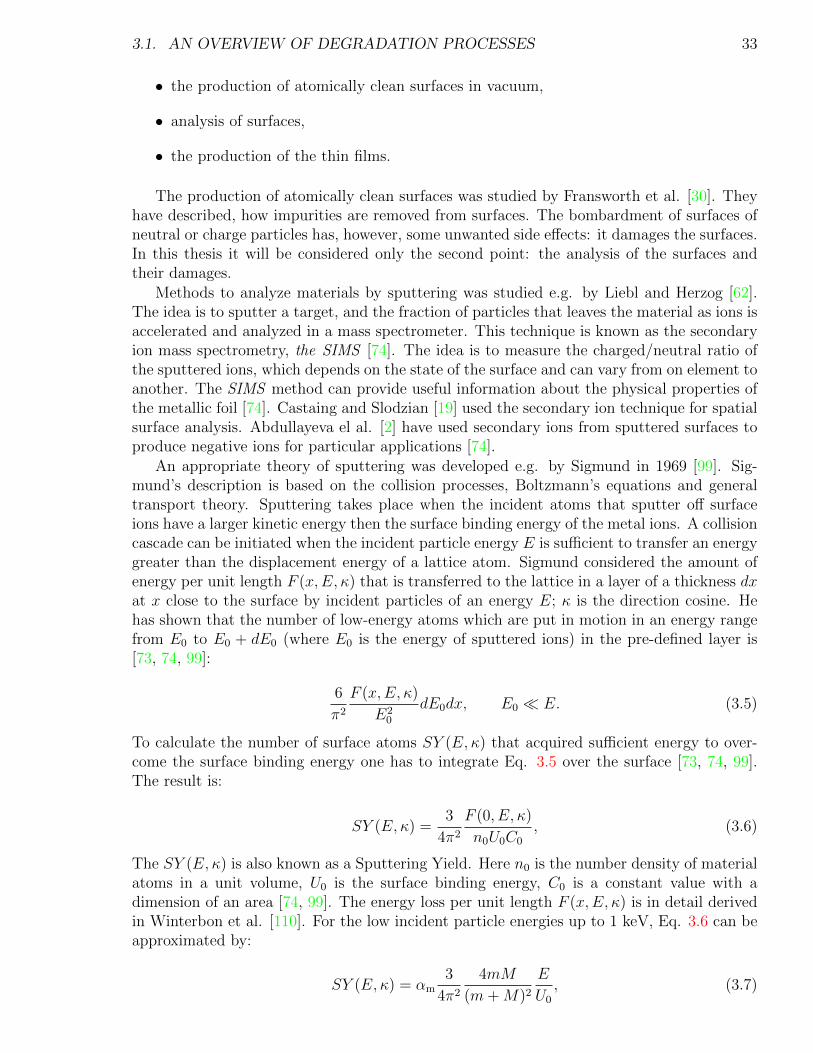
Figure 3.2: The sputtering yield as a function of angle θ [74].
The sputtering yield SY (θ) has its maximum at 70o ∼ 80o and then decreases to zero at 90o.This fact cannot be explained by use of here presented theory, because according to the Eq.3.9, SY (θ) is proportional to the secans of the angle θ [74]. However, the theory can explainthe phenomenon up to θ ≤ 80o, as it is seen in Fig. 3.2. For angles larger than 80o is not adominating degradation effect.
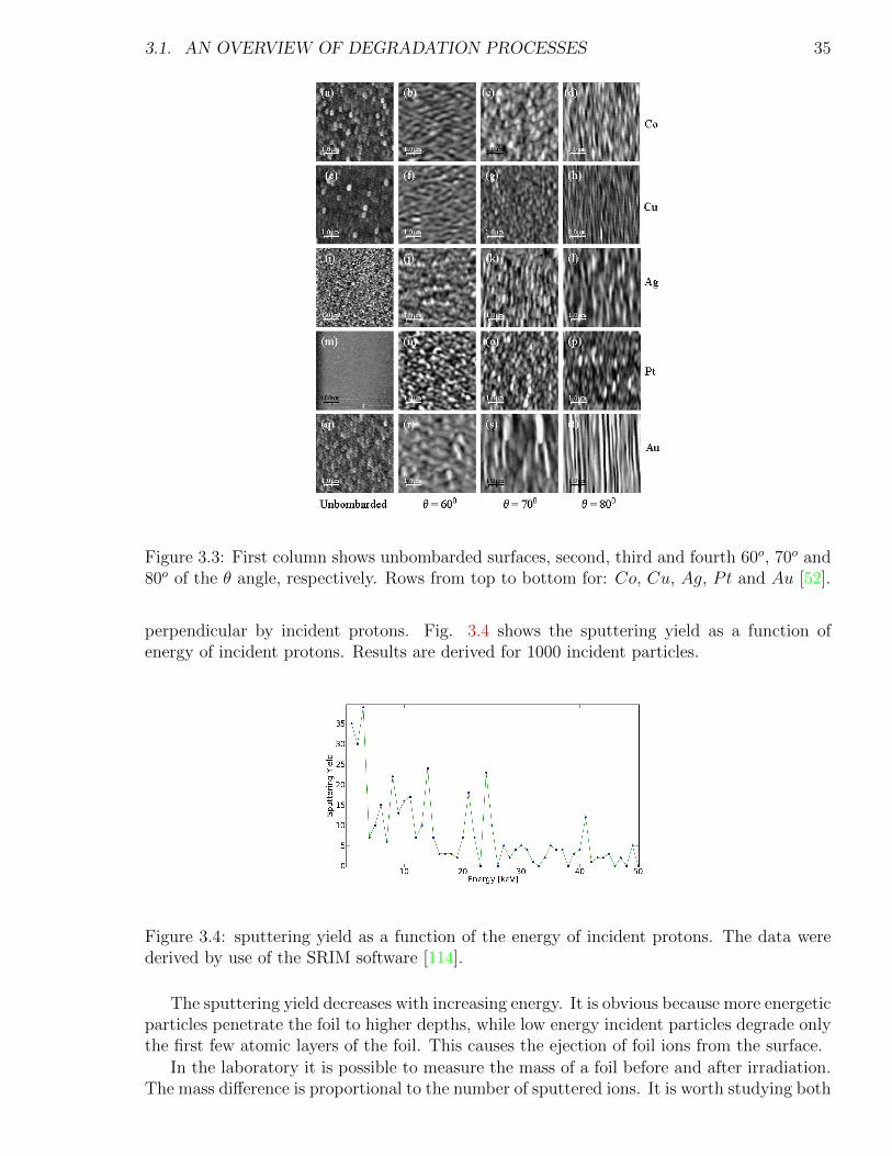
There exist many sputtering experiments. Karmakar et al. [52] investigated the sputteringon to a variety of thin metallic foils: Co, Cu, Ag, Pt and Au. The thickness of films variedin the range of 30 - 200 nm. The samples were exposed to ion fluences of 1× 10¹⁷ ions cm−2
for Co, Cu, Ag and Au and 5 × 10¹⁶ ions cm−2 for Pt of the 16.7 keV Ar+ ion beam. Thebase pressure in the target chamber was less than 5× 10⁻⁸ mbar [52]. Results are presentedin Fig. 3.3.
The first column shows unbombarded surfaces, while the second, third and fourth columnsshows surface bombarded under θ = 60o, 70o and 80o with above mention fluxes, respectively.At 60o riples appear for Co and Cu parallel to the ion beam direction. At 70o arrays of tinycones appear in the ion beam direction. At 80o characteristic ripples appear in all films [52].
By use of the SRIM software one can calculate the sputtering yield for a given anglebetween normal to the target and a beam line. 7.5 µm Kapton foil covered on both sideswith 100 nm Al, a typical solar sail material, was examined. The sample was irradiated
3.1. AN OVERVIEW OF DEGRADATION PROCESSES 35
Figure 3.3: First column shows unbombarded surfaces, second, third and fourth 60o, 70o and80o of the θ angle, respectively. Rows from top to bottom for: Co, Cu, Ag, Pt and Au [52].
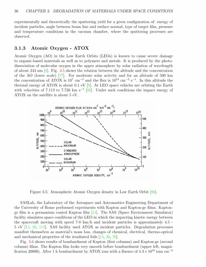
perpendicular by incident protons. Fig. 3.4 shows the sputtering yield as a function ofenergy of incident protons. Results are derived for 1000 incident particles.
Figure 3.4: sputtering yield as a function of the energy of incident protons. The data werederived by use of the SRIM software [114].
The sputtering yield decreases with increasing energy. It is obvious because more energeticparticles penetrate the foil to higher depths, while low energy incident particles degrade onlythe first few atomic layers of the foil. This causes the ejection of foil ions from the surface.
In the laboratory it is possible to measure the mass of a foil before and after irradiation.The mass difference is proportional to the number of sputtered ions. It is worth studying both
36 CHAPTER 3. DEGRADATION OF MATERIALS UNDER SPACE CONDITIONS
experimentally and theoretically the sputtering yield for a given configuration of: energy ofincident particles, angle between beam line and surface normal, type of target film, pressureand temperature conditions in the vacuum chamber, where the sputtering processes areobserved.
3.1.3 Atomic Oxygen - ATOX
Atomic Oxygen (AO) in the Low Earth Orbits (LEOs) is known to cause severe damageto organic-based materials as well as to polymers and metals. It is produced by the photo-dissociation of molecular oxygen in the upper atmosphere by solar radiation of wavelengthof about 243 nm [8]. Fig. 3.5 shows the relation between the altitude and the concentrationof the AO (lower scale) [77]. For moderate solar activity and for an altitude of 500 kmthe concentration of ATOX is 107 cm−3 and the flux is 1013 cm−2 s−1. In this altitude thethermal energy of ATOX is about 0.1 eV [8]. At LEO space vehicles are orbiting the Earthwith velocities of 7.113 to 7.726 km s−1 [80]. Under such conditions the impact energy ofATOX on the satellite is about 5 eV.
Figure 3.5: Atmospheric Atomic Oxygen density in Low Earth Orbit [90].
SASLab, the Laboratory of the Aerospace and Astronautics Engineering Department ofthe University of Rome performed experiments with Kapton and Kapton-ge films. Kapton-ge film is a germanium coated Kapton film [14]. The SAS (Space Environment Simulator)facility simulates space conditions of the LEO in which the impacting kinetic energy betweenthe spacecraft moving with speed 7-8 km/h and incident particles is approximately 4.5 -5 eV [14, 39, 112]. SAS facility used ATOX as incident particles. Degradation processesmanifest themselves as material’s mass loss, changes of chemical, electrical, thermo-opticaland mechanical properties of the irradiated foils [14, 38, 76].
Fig. 3.6 shows results of bombardment of Kapton (first columns) and Kapton-ge (secondcolumn) films. The Kapton film looks very smooth before bombardment (upper left, magni-fication 20000). After 1 h bombardment by ATOX ions with a fluence of 4.3×10¹⁸ ions cm−2
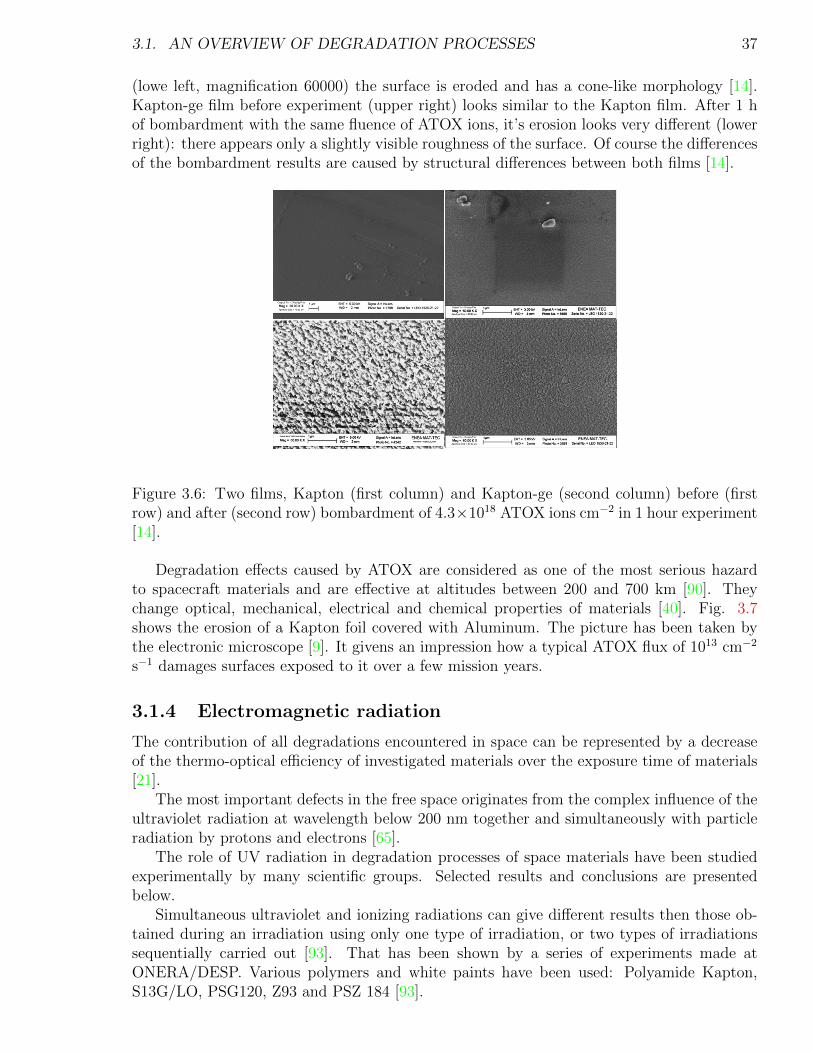
3.1. AN OVERVIEW OF DEGRADATION PROCESSES 37
(lowe left, magnification 60000) the surface is eroded and has a cone-like morphology [14].Kapton-ge film before experiment (upper right) looks similar to the Kapton film. After 1 hof bombardment with the same fluence of ATOX ions, it’s erosion looks very different (lowerright): there appears only a slightly visible roughness of the surface. Of course the differencesof the bombardment results are caused by structural differences between both films [14].
Figure 3.6: Two films, Kapton (first column) and Kapton-ge (second column) before (firstrow) and after (second row) bombardment of 4.3×10¹⁸ ATOX ions cm−2 in 1 hour experiment[14].
Degradation effects caused by ATOX are considered as one of the most serious hazardto spacecraft materials and are effective at altitudes between 200 and 700 km [90]. Theychange optical, mechanical, electrical and chemical properties of materials [40]. Fig. 3.7shows the erosion of a Kapton foil covered with Aluminum. The picture has been taken bythe electronic microscope [9]. It givens an impression how a typical ATOX flux of 1013 cm−2
s−1 damages surfaces exposed to it over a few mission years.
3.1.4 Electromagnetic radiation
The contribution of all degradations encountered in space can be represented by a decreaseof the thermo-optical efficiency of investigated materials over the exposure time of materials[21].
The most important defects in the free space originates from the complex influence of theultraviolet radiation at wavelength below 200 nm together and simultaneously with particleradiation by protons and electrons [65].
The role of UV radiation in degradation processes of space materials have been studiedexperimentally by many scientific groups. Selected results and conclusions are presentedbelow.
Simultaneous ultraviolet and ionizing radiations can give different results then those ob-tained during an irradiation using only one type of irradiation, or two types of irradiationssequentially carried out [93]. That has been shown by a series of experiments made atONERA/DESP. Various polymers and white paints have been used: Polyamide Kapton,S13G/LO, PSG120, Z93 and PSZ 184 [93].
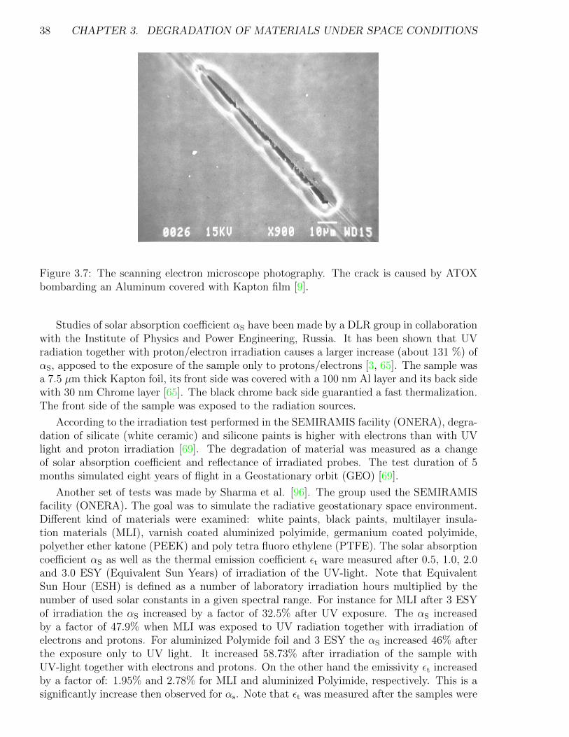
38 CHAPTER 3. DEGRADATION OF MATERIALS UNDER SPACE CONDITIONS
Figure 3.7: The scanning electron microscope photography. The crack is caused by ATOXbombarding an Aluminum covered with Kapton film [9].
Studies of solar absorption coefficient αS have been made by a DLR group in collaborationwith the Institute of Physics and Power Engineering, Russia. It has been shown that UVradiation together with proton/electron irradiation causes a larger increase (about 131 %) ofαS, apposed to the exposure of the sample only to protons/electrons [3, 65]. The sample wasa 7.5 µm thick Kapton foil, its front side was covered with a 100 nm Al layer and its back sidewith 30 nm Chrome layer [65]. The black chrome back side guarantied a fast thermalization.The front side of the sample was exposed to the radiation sources.
According to the irradiation test performed in the SEMIRAMIS facility (ONERA), degra-dation of silicate (white ceramic) and silicone paints is higher with electrons than with UVlight and proton irradiation [69]. The degradation of material was measured as a changeof solar absorption coefficient and reflectance of irradiated probes. The test duration of 5months simulated eight years of flight in a Geostationary orbit (GEO) [69].
Another set of tests was made by Sharma et al. [96]. The group used the SEMIRAMISfacility (ONERA). The goal was to simulate the radiative geostationary space environment.Different kind of materials were examined: white paints, black paints, multilayer insula-tion materials (MLI), varnish coated aluminized polyimide, germanium coated polyimide,polyether ether katone (PEEK) and poly tetra fluoro ethylene (PTFE). The solar absorptioncoefficient αS as well as the thermal emission coefficient εt ware measured after 0.5, 1.0, 2.0and 3.0 ESY (Equivalent Sun Years) of irradiation of the UV-light. Note that EquivalentSun Hour (ESH) is defined as a number of laboratory irradiation hours multiplied by thenumber of used solar constants in a given spectral range. For instance for MLI after 3 ESYof irradiation the αS increased by a factor of 32.5% after UV exposure. The αS increasedby a factor of 47.9% when MLI was exposed to UV radiation together with irradiation ofelectrons and protons. For aluminized Polymide foil and 3 ESY the αS increased 46% afterthe exposure only to UV light. It increased 58.73% after irradiation of the sample withUV-light together with electrons and protons. On the other hand the emissivity εt increasedby a factor of: 1.95% and 2.78% for MLI and aluminized Polyimide, respectively. This is asignificantly increase then observed for αs. Note that εt was measured after the samples were
3.2. BLISTERING 39
exposed to UV-light and irradiated by electrons and protons together.
Unfortunately, the group used the sequential irradiation of the samples, which meansthat the probe was first exposed to UV-light then αS was measured and after that the samesample was irradiated by electrons and protons and again αS was measured. This methoddoes not allow to examine the true role of degradation of the probe due to electrons/protonsirradiation alone, because the optical properties of the sample were already changed by thepreceding UV irradiation.
The space mission BepiColombo to planet Mercury planned and prepared by ESA togetherwith JAXA, provides a great opportunity to check the role of UV radiation in the degradationprocess of the protection shield of the spacecraft. Tests have been made in the ESA/ESTEClaboratories [45]. The shield has been produced with various silicate paints (white ceramic).Probes were irradiated by two types of UV radiation sources: a deuterium lamp (UV) and aVUV source. The UV wavelength bandwidth is 200 to 400 nm, while the VUV bandwidthis 115 to 200 nm. Probes were exposed at elevated (450oC) temperature to UV and VUVradiation of approximately 17 Solar Constants (SC), accumulating a total UV dose of 52000ESH [45]. Many types of white ceramic have been used (Astroquartz 2, Astroquartz 3 andNexel Refrex 1210), the increase of the solar absorptance αS varied from 353 % to 410% [45].
In summary, the optical properties (αS, εt) of different kinds of surfaces are damagedmore by exposure to UV-light then by electron/proton irradiation at least relatively shortdistances to the Sun [3, 65]. However, according to the studies accomplished by Marcoet al. [69] in a GEO orbit, electrons cause larger changes of optical properties of whiteceramic and silicone paints then UV-light together with proton irradiation. However in caseof aluminized Kapton and MLI blankets sequential irradiation with UV-light and chargeparticles has shown then the UV-light causes the main contribution to changes of the solarabsorption and the thermal emission coefficient [96]. Extreme environmental conditions likethose which are present at Mercury distance to the Sun were carefully studied at ESA/ESTEC[45]. The growth of the solar absorption coefficient of white ceramic due to UV radiationwas enormous. Unfortunately degradation effects due to particle irradiation were not takeninto account.
3.2 Blistering
H2 blisters are metal bubbles filled with hydrogen molecular gas resulting from recombinationprocesses in the metal lattice. Blistering occurs as an effect of irradiation damages. It changesthe physical properties of the irradiated surface and increases the erosion rate [7]. As it isknown from experiments, caps of blisters lose thermal contact with the target body and,therefore, become overheated under intensive beams [7]. Growth of blisters on a flat surfacecan be considered as the increase of surface roughness that causes the decrease of mirrorreflectivity [7].
Degradation of structural properties of solids, referred to as embrittlement caused byHydrogen, plays an important role in material physics [67]. Four general processes of theembrittlement have been proposed: formation of a hydride phase, enhanced local plasticity,grain boundary weakening, and blister/bubble formation [67, 81].
Blistering is caused by formation of pockets of hydrogen gas just below the metal sur-face. The tendency to form bubbles depends on: proton energy, time - integrated protonflux, temperature of the target, crystallographic orientation of the irradiated surface and onimpurities and defects in the sample [22]. The amount of Hydrogen retained in the sample
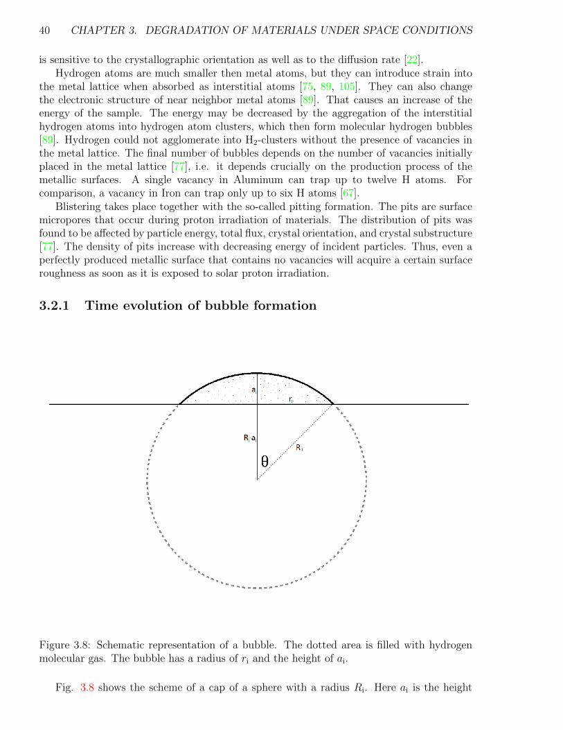
40 CHAPTER 3. DEGRADATION OF MATERIALS UNDER SPACE CONDITIONS
is sensitive to the crystallographic orientation as well as to the diffusion rate [22].Hydrogen atoms are much smaller then metal atoms, but they can introduce strain into
the metal lattice when absorbed as interstitial atoms [75, 89, 105]. They can also changethe electronic structure of near neighbor metal atoms [89]. That causes an increase of theenergy of the sample. The energy may be decreased by the aggregation of the interstitialhydrogen atoms into hydrogen atom clusters, which then form molecular hydrogen bubbles[89]. Hydrogen could not agglomerate into H2-clusters without the presence of vacancies inthe metal lattice. The final number of bubbles depends on the number of vacancies initiallyplaced in the metal lattice [77], i.e. it depends crucially on the production process of themetallic surfaces. A single vacancy in Aluminum can trap up to twelve H atoms. Forcomparison, a vacancy in Iron can trap only up to six H atoms [67].
Blistering takes place together with the so-called pitting formation. The pits are surfacemicropores that occur during proton irradiation of materials. The distribution of pits wasfound to be affected by particle energy, total flux, crystal orientation, and crystal substructure[77]. The density of pits increase with decreasing energy of incident particles. Thus, even aperfectly produced metallic surface that contains no vacancies will acquire a certain surfaceroughness as soon as it is exposed to solar proton irradiation.
3.2.1 Time evolution of bubble formation
Figure 3.8: Schematic representation of a bubble. The dotted area is filled with hydrogenmolecular gas. The bubble has a radius of ri and the height of ai.
Fig. 3.8 shows the scheme of a cap of a sphere with a radius Ri. Here ai is the height
3.2. BLISTERING 41
of the cap, while ri is it’s radius. Hereafter the cap is named as the bubble. By use of thespherical coordinates, the volume of the ith bubble is:
Vi =2
3πr3
i , (3.10)
For simplicity in this thesis a half sphere is considered, i.e. ai = Ri = ri. The general equationas well as the relation between the height and the radius of a cap of a sphere is presented inAppendix B.1.
The differential growth of the radius of the ith bubble dri is caused by a small portion ofH2 molecules merged to the bubble in a period of time dt.
It is assumed that the gas inside the ith bubble behaves like an ideal gas:
piVi =N∑j
NH2,i,jkBT, (3.11)
where pi is the pressure of the gas, kB is the Boltzmann constant, T denotes the temperatureof the sample, NH2,i,j is the number of H2 molecules merged to the ith bubble in the jth periodof time step ∆tj, N is the number of tiny time steps, hence N ×∆tj is the total irradiationtime of the sample. The number NH2,i,j is then given by:
NH2,i,j = 0.5(NT
B
)−1Np+,j η ξH2 (1−BS), NT
B = NBAs, Np+,j = I∆tjAs. (3.12)
The factor 0.5 reflects that a single H2 molecule consists of two H atoms, NTB is the total
number of bubbles on the irradiated sample, NB is the number of bubbles per unit area, Iis the proton flux, As is the area of the sample, Np+,j is the number of protons sent to thesample in the jth period of time step ∆tj. While 100% of protons recombine into H atoms inthe metal lattice, only a few percent of them recombine to H2 molecules [18]. Hence the ηfactor is the relation between the number of H2 molecules and the H atoms in the lattice. Notall of the H2 molecules will merge into a H2-clusters and finally to H2-bubbles, hence the ξH2
factor is the relation between the number of H2 molecules inside and outside the bubbles. BSis the factor of backscattered ions. If BS is 1 then all of the incident ions are backscattered.If BS is 0 then all of the incident ions penetrate into the target. BS depends on the protonenergy and on metal properties and can be estimated by use of the SRIM software [114].
The first step to estimate the radius of the ith bubble is to calculate the Helmholtz freeenergy of the whole configuration Fconfig. Since the free energy is an additive quantity, thetotal free energy of bubble formation is a sum of following constituents: free energy of H2
gas inside the ith bubble (Fgas,i), the metal deformation (Fmd,i) of the surface caused by thebubble itself, the surface free energy (Fsurf,i) of the cap of the bubble, free energy of H2
molecules (FH2), and that of the H atoms (FH) placed outside the bubbles within the metallattice.
The Helmholtz free energy of the whole configuration described above is:
Fconfig = Fgas,i + Fmd,i + Fsurf,i + FH2 + FH. (3.13)
The next step is to estimate the free energy of the increase of the ith bubble. It consists ofthe free energy of a gas filled in the bubble, the free energy of a metal deformation, and ofthe surface free energy of the bubble cap.
42 CHAPTER 3. DEGRADATION OF MATERIALS UNDER SPACE CONDITIONS
Using the well known thermodynamical relation between the pressure of the gas and theHelmholtz free energy, p =
(∂F∂V
)T
, together with Eq. 3.11, the free energy of a gas contained
in the ith bubble is:
Fgas,i = −N∑j
NH2,i,jkBT ln
(Vmax,i
Vmin
), (3.14)
where Vmax,i is the maximum volume a bubble can reach before it breaks, while Vmin is itsminimum volume.
It is assumed that two H2 molecules form the smallest possible bubble. The radius ofsuch bubble is approximately 3.2 Bohr radius [88].
The bubble will crack if the pressure of the gas inside is higher then the pressure exertedby the metal deformation of the cap. The relation between the pressure of the gas, the strainσs of the metal, and the bubble radius corresponding to Vmax,i is [61]:
pgas, insite bubble − poutside bubble =2σs
rmax,i
. (3.15)
Since it is assumed that the sample is placed in the space vacuum, the pressure outside thebubble is set to zero. The strain is a function of the temperature and it is unique for a givenmaterial. The maximum volume of the bubble is:
Vmax,i =2
3π
[3∑N
j NH2,i,jkBT
4πσs(T )
] 32
. (3.16)
The free energy of a metal deformation Fmd,i caused by the bubble with radius ri can befound in [58]. It is given by the following relation:
Fmd,i =4π
3
r3i (1 + γp)
EY
p2i . (3.17)
Here γp is the Poisson coefficient, i.e. the ratio of transverse to axial strain of the samplematerial, EY is the Young module. In Appendix B.4 in Table B.2 some Poisson coefficientsand Young modules for common materials are listed.
The free energy of a surface of a cap of the ith bubble can be found in [70]. It is given by:
Fsurf,i = 4πr2i σs(T ). (3.18)
The Helmholtz free energy of H2 molecules located outside the bubbles at certain positionswithin the metal lattice is expressed by the following relation:
FH2 =
NTH2−
NTB∑i
N∑j
NH2,i,j
εH2 + kBT ln
NTH2−∑NT
Bi
∑Nj NH2,i,j
N0
, (3.19)
where NTH2
is the total number of H2 molecules inside the sample, NTB is the total number
of bubbles on the sample, εH2 is the binding energy of the H2 molecule with a vacancy, andN0 is the number of the lattice sites. The detailed derivation of the Eq. 3.19 is presented inAppendix B.2.
Similarly, the Helmholtz free energy of H atoms located outside bubbles at certain posi-tions within the metal lattice is described by:
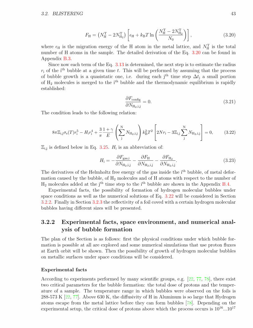
3.2. BLISTERING 43
FH =(NT
H − 2NTH2
) [εH + kBT ln
(NT
H − 2NTH2
N0
)], (3.20)
where εH is the migration energy of the H atom in the metal lattice, and NTH is the total
number of H atoms in the sample. The detailed derivation of the Eq. 3.20 can be found inAppendix B.3.
Since now each term of the Eq. 3.13 is determined, the next step is to estimate the radiusri of the ith bubble at a given time t. This will be performed by assuming that the processof bubble growth is a quasistatic one, i.e. during each jth time step ∆tj a small portionof H2 molecules is merged to the ith bubble and the thermodynamic equilibrium is rapidlyestablished:
∂Fconfig
∂NH2,i,j
= 0. (3.21)
The condition leads to the following relation:
8πΞi,jσs(T )r5i −Hir
4i +
3
π
1 + γ
E
N∑j
NH2,i,j
k2BT
2
2Nri − 3Ξi,j
N∑j
NH2,i,j
= 0, (3.22)
Ξi,j is defined below in Eq. 3.25. Hi is an abbreviation of:
Hi = − ∂Fgas,i
∂NH2,i,j
− ∂FH
∂NH2,i,j
− ∂FH2
∂NH2,i,j
. (3.23)
The derivatives of the Helmholtz free energy of the gas inside the ith bubble, of metal defor-mation caused by the bubble, of H2 molecules and of H atoms with respect to the number ofH2 molecules added at the jth time step to the ith bubble are shown in the Appendix B.4.
Experimental facts, the possibility of formation of hydrogen molecular bubbles underspace conditions as well as the numerical solutions of Eq. 3.22 will be considered in Section3.2.2. Finally in Section 3.2.3 the reflectivity of a foil coved with a certain hydrogen molecularbubbles having different sizes will be presented.
3.2.2 Experimental facts, space environment, and numerical anal-ysis of bubble formation
The plan of the Section is as follows: first the physical conditions under which bubble for-mation is possible at all are explored and some numerical simulations that use proton fluxesat Earth orbit will be shown. Then the possibility of growth of hydrogen molecular bubbleson metallic surfaces under space conditions will be considered.
Experimental facts
According to experiments performed by many scientific groups, e.g. [22, 77, 78], there existtwo critical parameters for the bubble formation: the total dose of protons and the temper-ature of a sample. The temperature range in which bubbles were observed on the foils is288-573 K [22, 77]. Above 630 K, the diffusivity of H in Aluminum is so large that Hydrogenatoms escape from the metal lattice before they can form bubbles [78]. Depending on theexperimental setup, the critical dose of protons above which the process occurs is 1016...1017
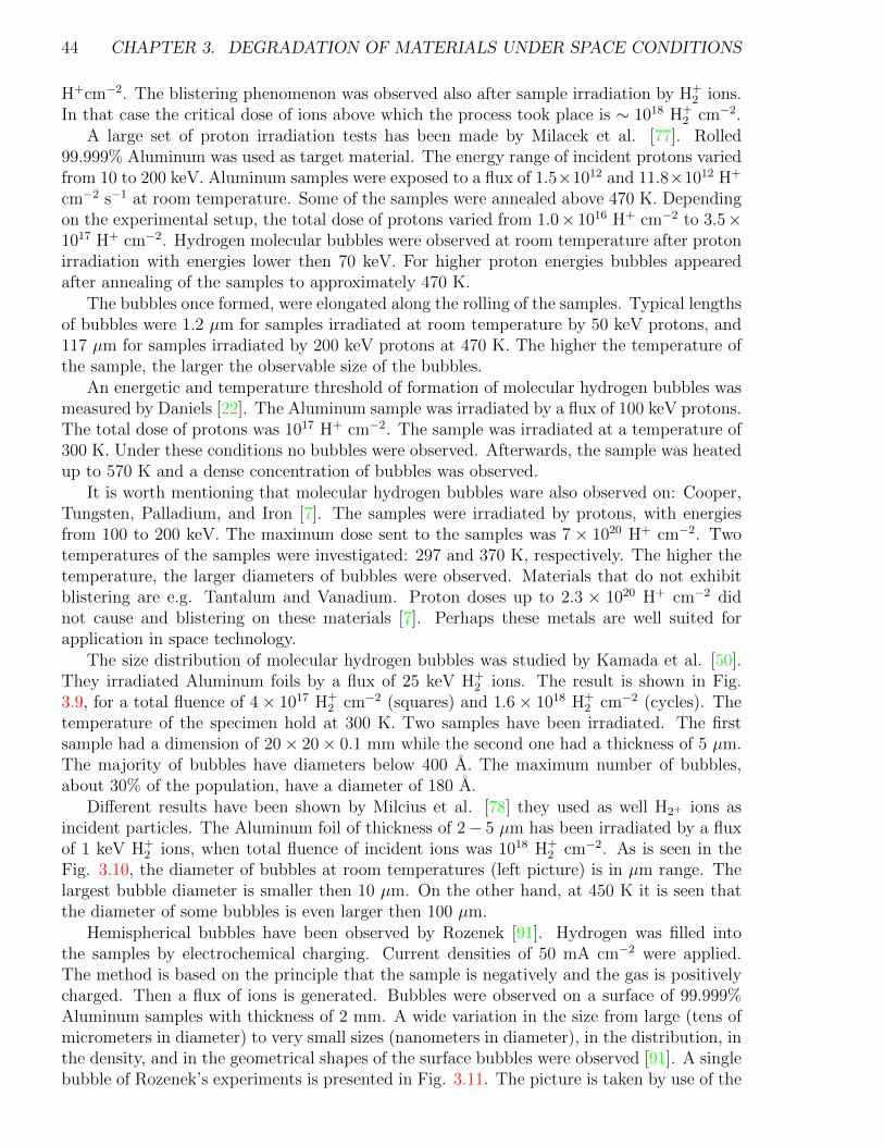
44 CHAPTER 3. DEGRADATION OF MATERIALS UNDER SPACE CONDITIONS
H+cm−2. The blistering phenomenon was observed also after sample irradiation by H+2 ions.
In that case the critical dose of ions above which the process took place is ∼ 1018 H+2 cm−2.
A large set of proton irradiation tests has been made by Milacek et al. [77]. Rolled99.999% Aluminum was used as target material. The energy range of incident protons variedfrom 10 to 200 keV. Aluminum samples were exposed to a flux of 1.5×10¹² and 11.8×10¹² H+
cm−2 s−1 at room temperature. Some of the samples were annealed above 470 K. Dependingon the experimental setup, the total dose of protons varied from 1.0× 10¹⁶ H+ cm−2 to 3.5×10¹⁷ H+ cm−2. Hydrogen molecular bubbles were observed at room temperature after protonirradiation with energies lower then 70 keV. For higher proton energies bubbles appearedafter annealing of the samples to approximately 470 K.
The bubbles once formed, were elongated along the rolling of the samples. Typical lengthsof bubbles were 1.2 µm for samples irradiated at room temperature by 50 keV protons, and117 µm for samples irradiated by 200 keV protons at 470 K. The higher the temperature ofthe sample, the larger the observable size of the bubbles.
An energetic and temperature threshold of formation of molecular hydrogen bubbles wasmeasured by Daniels [22]. The Aluminum sample was irradiated by a flux of 100 keV protons.The total dose of protons was 1017 H+ cm−2. The sample was irradiated at a temperature of300 K. Under these conditions no bubbles were observed. Afterwards, the sample was heatedup to 570 K and a dense concentration of bubbles was observed.
It is worth mentioning that molecular hydrogen bubbles ware also observed on: Cooper,Tungsten, Palladium, and Iron [7]. The samples were irradiated by protons, with energiesfrom 100 to 200 keV. The maximum dose sent to the samples was 7 × 10²⁰ H+ cm−2. Twotemperatures of the samples were investigated: 297 and 370 K, respectively. The higher thetemperature, the larger diameters of bubbles were observed. Materials that do not exhibitblistering are e.g. Tantalum and Vanadium. Proton doses up to 2.3 × 10²⁰ H+ cm−2 didnot cause and blistering on these materials [7]. Perhaps these metals are well suited forapplication in space technology.
The size distribution of molecular hydrogen bubbles was studied by Kamada et al. [50].They irradiated Aluminum foils by a flux of 25 keV H+
2 ions. The result is shown in Fig.3.9, for a total fluence of 4× 10¹⁷ H+
2 cm−2 (squares) and 1.6× 10¹⁸ H+2 cm−2 (cycles). The
temperature of the specimen hold at 300 K. Two samples have been irradiated. The firstsample had a dimension of 20× 20× 0.1 mm while the second one had a thickness of 5 µm.The majority of bubbles have diameters below 400 A. The maximum number of bubbles,about 30% of the population, have a diameter of 180 A.
Different results have been shown by Milcius et al. [78] they used as well H2+ ions asincident particles. The Aluminum foil of thickness of 2− 5 µm has been irradiated by a fluxof 1 keV H+
2 ions, when total fluence of incident ions was 1018 H+2 cm−2. As is seen in the
Fig. 3.10, the diameter of bubbles at room temperatures (left picture) is in µm range. Thelargest bubble diameter is smaller then 10 µm. On the other hand, at 450 K it is seen thatthe diameter of some bubbles is even larger then 100 µm.
Hemispherical bubbles have been observed by Rozenek [91]. Hydrogen was filled intothe samples by electrochemical charging. Current densities of 50 mA cm−2 were applied.The method is based on the principle that the sample is negatively and the gas is positivelycharged. Then a flux of ions is generated. Bubbles were observed on a surface of 99.999%Aluminum samples with thickness of 2 mm. A wide variation in the size from large (tens ofmicrometers in diameter) to very small sizes (nanometers in diameter), in the distribution, inthe density, and in the geometrical shapes of the surface bubbles were observed [91]. A singlebubble of Rozenek’s experiments is presented in Fig. 3.11. The picture is taken by use of the
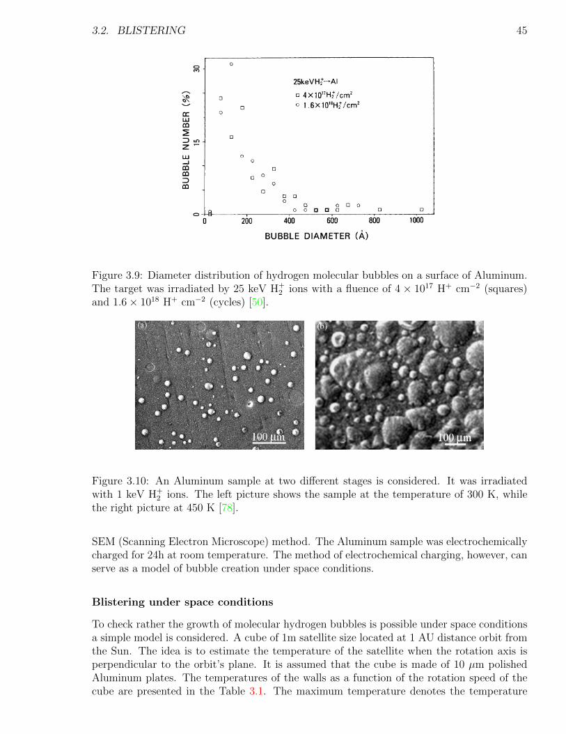
3.2. BLISTERING 45
Figure 3.9: Diameter distribution of hydrogen molecular bubbles on a surface of Aluminum.The target was irradiated by 25 keV H+
2 ions with a fluence of 4 × 10¹⁷ H+ cm−2 (squares)and 1.6× 10¹⁸ H+ cm−2 (cycles) [50].
Figure 3.10: An Aluminum sample at two different stages is considered. It was irradiatedwith 1 keV H+
2 ions. The left picture shows the sample at the temperature of 300 K, whilethe right picture at 450 K [78].
SEM (Scanning Electron Microscope) method. The Aluminum sample was electrochemicallycharged for 24h at room temperature. The method of electrochemical charging, however, canserve as a model of bubble creation under space conditions.
Blistering under space conditions
To check rather the growth of molecular hydrogen bubbles is possible under space conditionsa simple model is considered. A cube of 1m satellite size located at 1 AU distance orbit fromthe Sun. The idea is to estimate the temperature of the satellite when the rotation axis isperpendicular to the orbit’s plane. It is assumed that the cube is made of 10 µm polishedAluminum plates. The temperatures of the walls as a function of the rotation speed of thecube are presented in the Table 3.1. The maximum temperature denotes the temperature
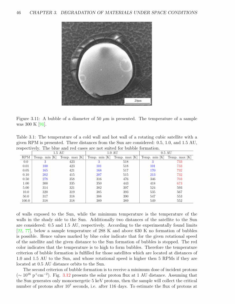
46 CHAPTER 3. DEGRADATION OF MATERIALS UNDER SPACE CONDITIONS
Figure 3.11: A bubble of a diameter of 50 µm is presented. The temperature of a samplewas 300 K [91].
Table 3.1: The temperature of a cold wall and hot wall of a rotating cubic satellite with agiven RPM is presented. Three distances from the Sun are considered: 0.5, 1.0, and 1.5 AU,respectively. The blue and red cases are not suited for bubble formation.
1.5 AU 1.0 AU 0.5 AURPM Temp. min [K] Temp. max [K] Temp. min [K] Temp. max [K] Temp. min [K] Temp. max [K]0.0 3 423 3 518 3 7330.01 100 423 101 518 101 7330.05 165 421 168 517 170 7320.10 202 415 207 515 213 7320.50 278 358 316 476 346 7031.00 300 335 350 443 418 6735.00 314 321 382 397 524 59310.0 320 319 385 393 535 56750.0 317 318 388 390 547 553100.0 318 318 389 389 549 552
of walls exposed to the Sun, while the minimum temperature is the temperature of thewalls in the shady side to the Sun. Additionally two distances of the satellite to the Sunare considered: 0.5 and 1.5 AU, respectively. According to the experimentally found limits[22, 77], below a sample temperature of 288 K and above 630 K no formation of bubblesis possible. Hence values marked by blue color indicate that for the given rotational speedof the satellite and the given distance to the Sun formation of bubbles is stopped. The redcolor indicates that the temperature is to high to form bubbles. Therefore the temperaturecriterion of bubble formation is fulfilled for those satellites which are located at distances of1.0 and 1.5 AU to the Sun, and whose rotational speed is higher then 5 RPMs if they arelocated at 0.5 AU distance orbits to the Sun.
The second criterion of bubble formation is to receive a minimum dose of incident protons(∼ 1016 p+cm−2). Fig. 3.12 presents the solar proton flux at 1 AU distance. Assuming thatthe Sun generates only monoenergetic 5 keV protons, then the sample will collect the criticalnumber of protons after 107 seconds, i.e. after 116 days. To estimate the flux of protons at
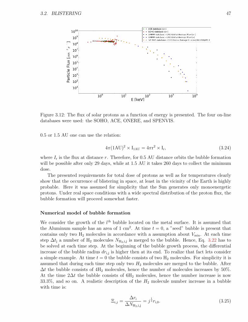
3.2. BLISTERING 47
Figure 3.12: The flux of solar protons as a function of energy is presented. The four on-linedatabases were used: the SOHO, ACE, ONERE, and SPENVIS.
0.5 or 1.5 AU one can use the relation:
4π(1AU)2 × I1AU = 4πr2 × Ir, (3.24)
where Ir is the flux at distance r. Therefore, for 0.5 AU distance orbits the bubble formationwill be possible after only 29 days, while at 1.5 AU it takes 260 days to collect the minimumdose.
The presented requirements for total dose of protons as well as for temperatures clearlyshow that the occurrence of blistering in space, at least in the vicinity of the Earth is highlyprobable. Here it was assumed for simplicity that the Sun generates only monoenergeticprotons. Under real space conditions with a wide spectral distribution of the proton flux, thebubble formation will proceed somewhat faster.
Numerical model of bubble formation
We consider the growth of the ith bubble located on the metal surface. It is assumed thatthe Aluminum sample has an area of 1 cm2. At time t = 0, a ”seed” bubble is present thatcontains only two H2 molecules in accordance with a assumption about Vmin. At each timestep ∆tj a number of H2 molecules NH2,i,j is merged to the bubble. Hence, Eq. 3.22 has tobe solved at each time step. At the beginning of the bubble growth process, the differentialincrease of the bubble radius dri,j is higher then at its end. To realize that fact lets considera simple example. At time t = 0 the bubble consists of two H2 molecules. For simplicity it isassumed that during each time step only two H2 molecules are merged to the bubble. After∆t the bubble consists of 4H2 molecules, hence the number of molecules increases by 50%.At the time 2∆t the bubble consists of 6H2 molecules, hence the number increase is now33.3%, and so on. A realistic description of the H2 molecule number increase in a bubblewith time is:
Ξi,j =∆ri
∆NH2,i,j
= j13 ri,0. (3.25)
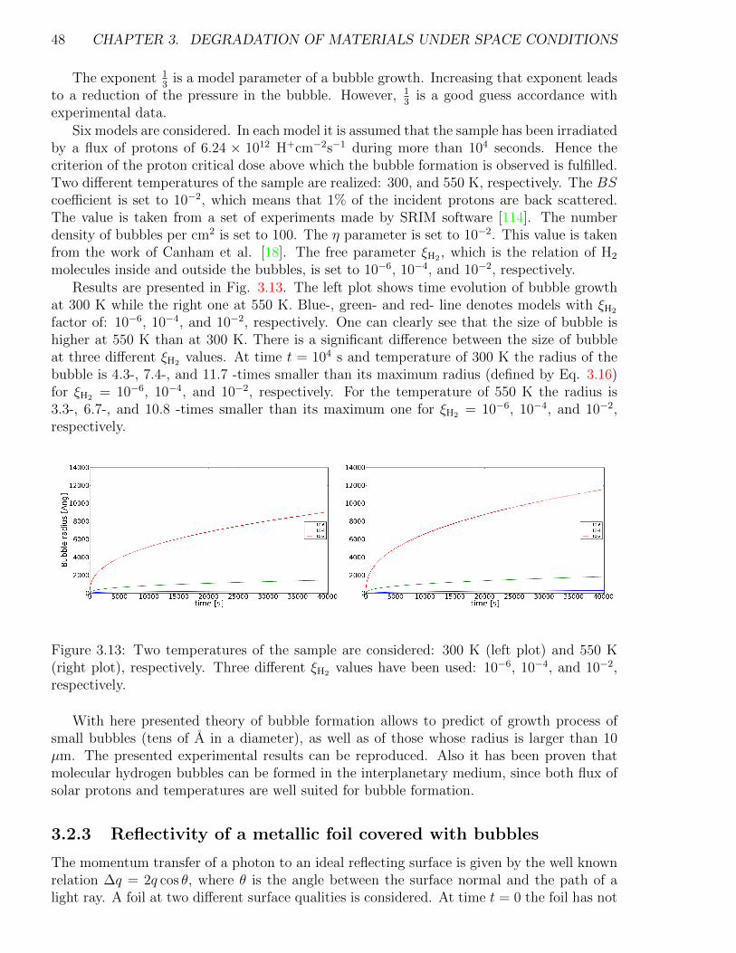
48 CHAPTER 3. DEGRADATION OF MATERIALS UNDER SPACE CONDITIONS
The exponent 13
is a model parameter of a bubble growth. Increasing that exponent leadsto a reduction of the pressure in the bubble. However, 1
3is a good guess accordance with
experimental data.Six models are considered. In each model it is assumed that the sample has been irradiated
by a flux of protons of 6.24 × 10¹² H+cm−2s−1 during more than 104 seconds. Hence thecriterion of the proton critical dose above which the bubble formation is observed is fulfilled.Two different temperatures of the sample are realized: 300, and 550 K, respectively. The BScoefficient is set to 10−2, which means that 1% of the incident protons are back scattered.The value is taken from a set of experiments made by SRIM software [114]. The numberdensity of bubbles per cm2 is set to 100. The η parameter is set to 10−2. This value is takenfrom the work of Canham et al. [18]. The free parameter ξH2 , which is the relation of H2
molecules inside and outside the bubbles, is set to 10−6, 10−4, and 10−2, respectively.Results are presented in Fig. 3.13. The left plot shows time evolution of bubble growth
at 300 K while the right one at 550 K. Blue-, green- and red- line denotes models with ξH2
factor of: 10−6, 10−4, and 10−2, respectively. One can clearly see that the size of bubble ishigher at 550 K than at 300 K. There is a significant difference between the size of bubbleat three different ξH2 values. At time t = 104 s and temperature of 300 K the radius of thebubble is 4.3-, 7.4-, and 11.7 -times smaller than its maximum radius (defined by Eq. 3.16)for ξH2 = 10−6, 10−4, and 10−2, respectively. For the temperature of 550 K the radius is3.3-, 6.7-, and 10.8 -times smaller than its maximum one for ξH2 = 10−6, 10−4, and 10−2,respectively.
Figure 3.13: Two temperatures of the sample are considered: 300 K (left plot) and 550 K(right plot), respectively. Three different ξH2 values have been used: 10−6, 10−4, and 10−2,respectively.
With here presented theory of bubble formation allows to predict of growth process ofsmall bubbles (tens of A in a diameter), as well as of those whose radius is larger than 10µm. The presented experimental results can be reproduced. Also it has been proven thatmolecular hydrogen bubbles can be formed in the interplanetary medium, since both flux ofsolar protons and temperatures are well suited for bubble formation.
3.2.3 Reflectivity of a metallic foil covered with bubbles
The momentum transfer of a photon to an ideal reflecting surface is given by the well knownrelation ∆q = 2q cos θ, where θ is the angle between the surface normal and the path of alight ray. A foil at two different surface qualities is considered. At time t = 0 the foil has not
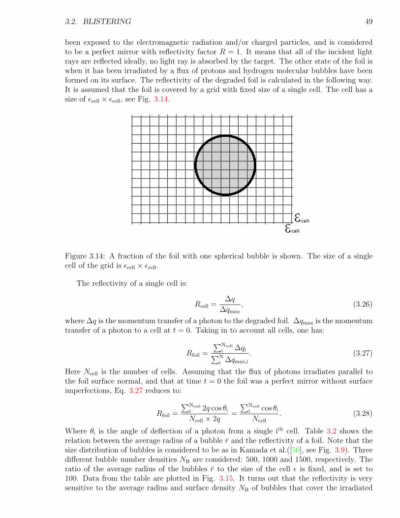
3.2. BLISTERING 49
been exposed to the electromagnetic radiation and/or charged particles, and is consideredto be a perfect mirror with reflectivity factor R = 1. It means that all of the incident lightrays are reflected ideally, no light ray is absorbed by the target. The other state of the foil iswhen it has been irradiated by a flux of protons and hydrogen molecular bubbles have beenformed on its surface. The reflectivity of the degraded foil is calculated in the following way.It is assumed that the foil is covered by a grid with fixed size of a single cell. The cell has asize of εcell × εcell, see Fig. 3.14.
Figure 3.14: A fraction of the foil with one spherical bubble is shown. The size of a singlecell of the grid is εcell × εcell.
The reflectivity of a single cell is:
Rcell =∆q
∆qmax
, (3.26)
where ∆q is the momentum transfer of a photon to the degraded foil. ∆qmax is the momentumtransfer of a photon to a cell at t = 0. Taking in to account all cells, one has:
Rfoil =
∑Ncell
i ∆qi∑Ni ∆qmax,i
. (3.27)
Here Ncell is the number of cells. Assuming that the flux of photons irradiates parallel tothe foil surface normal, and that at time t = 0 the foil was a perfect mirror without surfaceimperfections, Eq. 3.27 reduces to:
Rfoil =
∑Ncell
i 2q cos θi
Ncell × 2q=
∑Ncell
i cos θi
Ncell
. (3.28)
Where θi is the angle of deflection of a photon from a single ith cell. Table 3.2 shows therelation between the average radius of a bubble r and the reflectivity of a foil. Note that thesize distribution of bubbles is considered to be as in Kamada et al.([50], see Fig. 3.9). Threedifferent bubble number densities NB are considered: 500, 1000 and 1500, respectively. Theratio of the average radius of the bubbles r to the size of the cell ε is fixed, and is set to100. Data from the table are plotted in Fig. 3.15. It turns out that the reflectivity is verysensitive to the average radius and surface density NB of bubbles that cover the irradiated
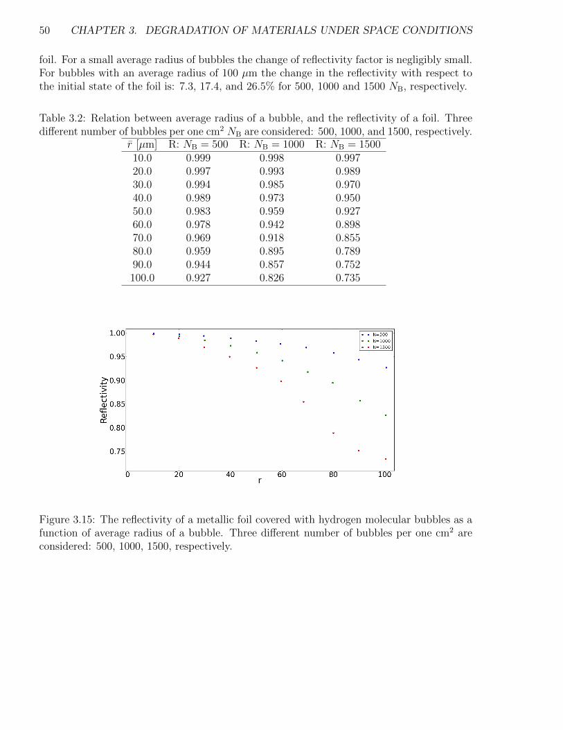
50 CHAPTER 3. DEGRADATION OF MATERIALS UNDER SPACE CONDITIONS
foil. For a small average radius of bubbles the change of reflectivity factor is negligibly small.For bubbles with an average radius of 100 µm the change in the reflectivity with respect tothe initial state of the foil is: 7.3, 17.4, and 26.5% for 500, 1000 and 1500 NB, respectively.
Table 3.2: Relation between average radius of a bubble, and the reflectivity of a foil. Threedifferent number of bubbles per one cm2 NB are considered: 500, 1000, and 1500, respectively.
r [µm] R: NB = 500 R: NB = 1000 R: NB = 150010.0 0.999 0.998 0.99720.0 0.997 0.993 0.98930.0 0.994 0.985 0.97040.0 0.989 0.973 0.95050.0 0.983 0.959 0.92760.0 0.978 0.942 0.89870.0 0.969 0.918 0.85580.0 0.959 0.895 0.78990.0 0.944 0.857 0.752100.0 0.927 0.826 0.735
Figure 3.15: The reflectivity of a metallic foil covered with hydrogen molecular bubbles as afunction of average radius of a bubble. Three different number of bubbles per one cm2 areconsidered: 500, 1000, 1500, respectively.
Chapter 4
Conclusions and Outlooks
This thesis explained the importance of degradation processes of materials under space con-ditions. The space environment is highly rough for any technical equipment, since space isfilled with high speed charge particles and electromagnetic radiation. In this thesis the solarsail technology was used as a reference example. The performance of sail-crafts is slightlydefected to any changes of thermo-optical properties of their materials, since their propulsionabilities suffers from any degradation processes.
A short review of the most important degradation processes was given. A possibility ofcharge of metallic foils under particle irradiation was investigated. The following degradationprocesses that may appear in space have been discussed: the sputtering process, influence ofthe Atomic Oxygen, and effects of electromagnetic irradiation.
Recombination processes of incident protons with metal free electrons were investigatedwith special attention. A detailed mathematical description of the following three processeswas presented: the Auger-, the resonant-, and the Oppenheimer-Brinkman-Kramers (OBK)-process, respectively. The author modified the OBK process that it is now suited for lightincident ions. That is the case when metallic targets are irradiated by solar protons.
The central topic of this thesis was the development of a thermodynamical model offormation of molecular hydrogen bubbles on metallic surfaces under space conditions. Thehere presented model allows the description of bubble grow on selected materials and underwell defined environmental conditions. The grow both of small bubbles (tens of A in diameter)and larger ones (tens in µm in a diameter) can be modeled. The reflectivity of the Aluminumfoil that is covered with different bubble surface densities and different radii was investigated.A quantitative relation between the bubble growth, the bubble surface density, and thereflectivity of the degraded foil has been derived. Therefore, bubble formation will reducethe propulsion abilities of any sail-craft.
Thus up to now available results of laboratory experiments with respect to molecularbubble growth under proton irradiation have been reviewed. A large set of different materialshas been investigated. The collected experimental results and the numerical model lead tothe conclusion that bubble growth processes may appear at least in the close vicinity of theSun.
In the near future the formation theory of molecular hydrogen bubbles on metallic surfaceswill be verified experimentally by use of the Complex Irradiation Facility (hereafter CIF) atDLR, Bremen, Germany. This facility is designed to study the behavior of materials undercomplex irradiation and to investigate their degradation in the space environment. Withthe CIF it is possible to irradiate samples with three light sources (for the simulation of thespectrum of solar electromagnetic radiation) simultaneously with protons and electrons.
51
52 CHAPTER 4. CONCLUSIONS AND OUTLOOKS
Further theoretical studies of the bubble growth process are planned. Different equationsof state of the hydrogen molecular gas will be tested. It would be interesting to study thedynamics of bubble growth with different gas models. A more sophisticated mechanism ofbubble crack will be implemented. The idea is to take into account the dynamical thicknesschange of a bubble cap. Also a broad variation of merging process of H2 molecules to abubble will be studied.
Since for the foreseeable future no sample returns of materials exposed to interplanetaryspace is planned, both laboratory, and theoretical studies of degradation processes that arebased on Hydrogen recombination are considered. They are nevertheless necessary, sincebubble formation can be a serious problem for the success of space missions.
Appendix A
OBK recombination in metal lattices
A.1 The Hartree approximation
One can consider a multiparticle system described by a Hamiltonian (all particles are distin-guishable) in the form:
H =∑
i
Hi +1
2
∑i6=j
Vi,j, (A.1)
where Hi =p2
i
2m+ Vs(ri) and Vi,j = Vint(| ri − rj |), here Vs is the single-particle potential and
Vint is the interaction potential [71].In the Hartree approximation, one assumes that the wavefunction of eigenstates of the
Hamiltonian can be written as a product of wavefunctions of single particle states, thus [71]:
Φ = φ1(r1) φ2(r2) φ3(r3) ... (A.2)
The expectation value of the Hamiltonian will have the form:∫d3r1d
3r2 ... φ∗1(r1)φ∗2(r2) ...
(∑i
Hi +1
2
∑i 6=j
Vi,j
)φ1(r1)φ2(r2) ... (A.3)
Thus one can realize that the sum over Hi and Vi,j reduces to one and two particle expectationvalues [71]. Taking the functional derivative of the above equation with respect to φ∗m(rm)for the mth partcile, one has:
∫d3rm
(Hmφm(rm) +
∑i 6=m
∫d3riφ
∗i (ri)Vi,mφi(ri)φm(rm)− Eφ∗m(rm)
)δφ∗m(rm) = 0 (A.4)
Thus one can write Eq. A.4 in the form:
Hmφm(rm) +
(∑i 6=m
∫d3riφ
∗i (ri) Vi,m φi(ri)
)φm(rm) = Eφm(rm). (A.5)
Stationary Schroedinger equation A.5 is called the Hartree equation [71]. Hartree approx-imation reduces a N -particle problem to a set of single equations that one can solve. Theinteraction between the particles is reduced to a single potential potential [71]:
53
54 APPENDIX A. OBK RECOMBINATION IN METAL LATTICES
VH(rm) =
∫d3ri
∑i 6=m
| φi(ri) |2 Vint(ri − rm). (A.6)
Equation A.6 describes the interaction of the mth particle with all other particles. If oneconsider a Coulomb interaction between the particles, the Hartree potential looks like theinteraction of one particle with the charge density of all other particles [71]:
VH(rm) =
∫d3r
ZtZpρm(r)
| rm − r |. (A.7)
Here ρm(r) is the probability density that the mth particle is located at position r. Zt and Zp
are a charge numbers of target ions and incident ions, respectively. The mth particle dependson the states of all the other N − 1 particles.
A.2 The ionization energy of an electron in the 1s state
- the OBK process
The ionization energy of an electron in the 1s state is:
− IK = E(α,C) = 〈φi(r1) | H | φi(r1)〉, (A.8)
where the Hamiltonian and the wave function are:
H = −1
2∇2 − 1
r1
− (Zt − 1)
r1
exp(−Cr1), (A.9)
φi(r1) = π−12α
32 exp(−αr1). (A.10)
To calculate the ionization energy one can use the spherical coordinate system. Forsimplicity one can consider each term of Eq. A.9 separately:
1. 〈φi(r1) | −12∇2 | φi(r1)〉:
〈φi(r1) | −1
2∇2 | φi(r1)〉 = −1
2〈φi(r1) |
[−π−
12α
52
2
r1
exp(−αr1) + π−12α
72 exp(−αr1)
].
(A.11)
The first term in the Eq. A.11 is:
−12
∫V
π−12α
32 exp(−αr1)
[−π−
12α
52
2
r1
exp(−αr1)
]dV = (A.12)
4α4
∫ ∞0
r1 exp(−2αr1) dr1 = −α2 2αr1 + 1
exp(2αr1)|∞0 =
−α2 1
1 + (2αr1)2
2(1+2αr1)+ (2αr1)3
6(1+2αr1)+ ...
|∞0 = α2,
and the second one is:
A.3. CROSS SECTION OF THE OBK PROCESS 55
−12
∫V
π−12α
32 exp(−αr1)
[π−
12α
72 exp(−αr1)
]dV = (A.13)
−2α5
[exp(−2αr1)
(r2
1
−2α− 2r1
4α2− 1
4α3
)]|∞0 = −1
2α2.
So the term 〈φi(r1) | −12∇2 | φi(r1)〉 = 1
2α2.
2. 〈φi(r1) | − 1r1| φi(r1)〉:
〈φi(r1) | − 1
r1
| φi(r1)〉 = −4α3
∫ ∞0
r1 exp(−2αr1) dr1 = (A.14)
α2αr1 + 1
exp(2αr1)|∞0 = α
1
1 + (2αr1)2
2(2αr1+1)+ (2αr1)3
6(2αr1+1)+ ...
|∞0 = −α
3. 〈φi(r1) | − (Zt−1)r1
exp(−Cr1) | φi(r1)〉:
〈φi(r1) | −(Zt − 1)
r1
exp(−Cr1) | φi(r1)〉 = (A.15)
−4(Zt − 1)α3
∫ ∞0
r1 exp[−(C + 2α)r1] dr1 =
4(Zt − 1)α3 exp[−(C + 2α)r1]
(C + 2α)2[(C + 2α)r1 + 1] |∞0 =
4(Zt − 1)α3
(C + 2α2)2
1
1 + [(C+2α)r1]2
2[1+(C+2α)r1]+ ...
=
−4(Zt − 1)α3
(C + 2α)2
Thus, ionization energy of the electron in the 1s state is the sum of three terms calculatedabove:
− IK =1
2α2 − α− 4(Zt − 1)
α3
(C + 2α)2(A.16)
A.3 Cross section of the OBK process
The initial and final wave functions of the active electron are:
ψi(r1, t) = φi(r1) exp
(−ipv · r− i1
2p2v2t
), (A.17)
ψf(r2, t) = φ2(r2) exp
[i(1− p)v · r− i
2(1− p)2v2t
], (A.18)
where:
56 APPENDIX A. OBK RECOMBINATION IN METAL LATTICES
φi(r1) = π−12α
32 exp(−αr1), (A.19)
φf(r2) = π−12Z
32p exp(−Zpr2). (A.20)
Here p = mp/(mp − mt), r1 = r + pR, and r2 = r − (1 − p)R, and R = b + vt. If themass of the incident ion is small compared to the mass of the target atom (p = 0.036 forAl as a target and p+ as an incident ion) one can set the p parameter to zero. For thatapproximation r1 and r2 are, respectively:
r1∼= r, (A.21)
r2∼= r−R. (A.22)
Thus the wave functions are:
ψi(r1, t) ∼= φi(r1), (A.23)
ψf(r2 = r−R, t) ∼= φ2(r2 = r−R)× exp
[iv · r− i
2v2t
]. (A.24)
The Hamiltonian of the active electron is:
H = −1
2∇2
r −α
r+ Vs, (A.25)
where Vs is the effective potential felt by the active electron (see Eq. 2.91):
Vs = − Zp
r − b− vt+
1
r[(α− 1)− (Zt − 1) exp(−Cr)] . (A.26)
To calculate the cross section of the process [25] one has first to evaluate the so-called tran-sition amplitude [55]:
A(b) =1
i
∫ ∞−∞
dt 〈ψf | Vs | ψi〉, (A.27)
Σ ∼∫ ∞
0
db | A(b) |2 b. (A.28)
The first step will be to calculate the 〈ψf | Vs | ψi〉 term:
〈ψf | Vs | ψi〉 = 〈ψf |[− Zpr − b− vt
+α− 1
r− Zt − 1
rexp(−cr)
]| π−
12α
32 exp(−Cr)〉,
(A.29)
For simplicity one can consider each term separately:
1. The 〈ψf | − Zpr−b−vt | ψi〉
A.3. CROSS SECTION OF THE OBK PROCESS 57
〈ψf | −Zp
r − b− vt| ψi〉 = (A.30)
−4Z52p α
32 exp
[Zp(b+ vt)− i
2v2t
] ∫ ∞0
r2 exp[r(iv − α− Zp)]
r − b− vtdr =
8Z52p α
32
exp(ZpR− i2v2t)
R(α + Zp − iv)3
2. 〈ψf | α−1r| ψi〉:
〈ψf |α− 1
r| ψi〉 = (A.31)
4Z32p α
32 (α− 1) exp
(ZpR−
i
2v2t
)∫ ∞0
r exp[r(iv − Zp − α)] dr =
4Z32p α
32 (α− 1)
exp(ZpR− i2v2t)
(iv − Zp − α)2
3. 〈ψf | −Zt−1r
exp(−cr) | ψi〉:
〈ψf | −Zt − 1
rexp(−Cr) | ψi〉 =(A.32)
−4Z32p α
32 (Zt − 1) exp
(ZpR−
i
2v2t
)∫ ∞0
r exp [r(−Zp + iv − C − α)] dr =
−4Z32p α
32 (Zt − 1)
exp(ZpR− i
2v2t)
(Zp + C + α− iv)2
So, the matrix element i.e. the transition probability from the initial to the final state〈ψf | Vs | ψi〉 is:
〈ψf | Vs | ψi〉 = 4Z32p α
52 exp
(ZpR−
i
2v2t
)× (A.33)
×[− 2Zp
αR(iv − Zp − α)3+
1− α−1
(iv − Zp − α)2+
Zt − 1
α(α + Zp + C − iv)2
].
The scattering amplitude is defined as the time integral over this matrix element:
A(b) =1
i
∫ ∞−∞
dt 〈ψf | Vs | ψi〉 =(A.34)
23Z52p α
32 exp(Zpb)
i(Zp − i2v)v
− 2
b(iv − Zp − α)3α
[1− 1
b(Zp − i2v)
]+
1− α−1
(iv − α− Zp)2+
Zt − 1
α(α+ Zp + C − iv)2
.
From Eq. A.28 suggests that the cross section of the OBK process depends strongly onthe incident proton velocity Σ ∼ v−12. As it was mentioned in the Section 2.4.3, the OBKprocess has an energetic threshold above which it occurs. It is efficient for high energy ionswith energies of some MeVs.

58 APPENDIX A. OBK RECOMBINATION IN METAL LATTICES
Appendix B
Formation of hydrogen molecularbubbles on metal surfaces
B.1 Volume of a cap of a sphere
Using the geometry shown in the Fig. 3.8 and the spherical coordinates, the volume of a capof a sphere (hereafter the bubble) is:
V =
∫ R
0
∫ θ
0
∫ 2π
0
R′2
sin θ′ dR′dθ′dφ, (B.1)
V =2π
3R3(1− cos θ). (B.2)
Given the relation between radius r and height a of the bubble, R = 12a
(r2 + a2), the volumeis:
V =π
12
[r2 + a2
a
]3
(1− cos θ). (B.3)
The relation between the height and the radius of the bubble is:
a = r
(1− cos θ
sin θ
). (B.4)
If θ is set to 0 then a = r = R = 0, on the other hand if the θ angle is π/2 then a = r = R.
B.2 Helmholtz free energy of H2 molecules placed in
certain positions in the sample’s lattice
To get the relation of the Helmholtz free energy of the H2 molecules located at certainpositions in the sample but outside the bubbles, the definition of the free energy is used:
F = E − TS, S = kB ln Ω, (B.5)
here E is the internal energy of the H2 molecules located at certain positions in the metallattice, S denotes the entropy, while Ω represents the number of ways in which the H2
molecules can be arranged on the N0 lattice sites.
59
60APPENDIX B. FORMATIONOF HYDROGENMOLECULAR BUBBLES ONMETAL SURFACES
The number of lattice sites can be expressed by:
N0 = NAdCSDAA2
s
Mu
, (B.6)
where dCSDA is the CSDA range of the fastest incident proton [114], As is the irradiated areaof the sample, and Mu is the molar mass of the sample’s material.
The number of H2 molecules located outside the bubbles at certain positions in the metal
lattice is NTH2−∑NT
Bi
∑Nit
j NH2,i,j. Where NTH2
is the total number of H2 molecules in the
sample, while∑NT
Bi
∑Nit
j NH2,i,j is the total number of H2 molecules within all bubbles. The
summation over the number of time steps j count the number of H2 molecules in the ith bubble.The second summation over the number of bubble ith, counts the number of H2 moleculeswithin all bubbles. Therefore, performing the subtraction one gets the total number of H2
molecules outside all bubbles, located at certain positions in the metal lattice. The entropykB lnW of the collection of the H2 molecules placed on a lattice site is [108]:
S = kB lnN0!(
NTH2−∑NT
Bi
∑Nj dNH2,i,j
)![N0 −
(NT
H2−∑NT
Bi
∑Nj NH2,i,j
)]!, (B.7)
∼= −kB
NTH2−
NTB∑i
N∑j
NH2,i,j
ln
NTH2−∑NT
Bi
∑Nj NH2,i,j
N0
.The internal energy E is given by the following relation:
E = εH2
NTH2−
NTB∑i
N∑j
NH2,i,j
, (B.8)
where εH2 is the binding energy of the H2 molecule to a vacancy [67]. The internal energy ofH2 molecules located in the metal lattice sites is a product of the binding energy of a singleH2 molecule and the number of molecules.
The Helmholtz free energy of the H2 molecules located outside the bubbles at certainpositions in the metal lattice is then:
FH2 =
NTH2−
NTB∑i
N∑j
NH2,i,j
ε+ kBT ln
NTH2−∑NT
Bi
∑Nj NH2,i,j
N0
. (B.9)
B.3 Helmholtz free energy of H atoms in the sample
The number of H atoms in the sample and outside the bubbles is:
NH = NTH − 2
(NB∑
i
N∑j
NH2,i,j +Nout. bubblesH2
), (B.10)
where NTH is the total number of H atoms in the sample, so the number counts all of the
incident hydrogen ions which have recombined into hydrogen atoms. Some of the hydrogen
B.4. THE DERIVATIVES OF HELMHOLTZ FREE ENERGYOF: GAS OF THE ITH BUBBLE, METAL DEFORMATION CAUSED BY THE BUBBLE, H2 MOLECULES, AND H ATOMS LOCATEDOUTSIDE THE BUBBLES.61
atoms have recombined to H2 molecules and some of the molecules are forming the bubbles.Hence to get the number of H atoms located on the lattice sites one has to subtract the totalthe total number of hydrogen atoms NT
H and those hydrogen atoms which build H2 clustersand H2 bubbles. The reason of the factor 2 is that a single H2 molecule consists of two Hatoms.
The procedure to estimate the Helmholtz free energy of H atoms in the sample is thesame as in Eq. B.9. Hence the term is:
FH = NH
(εH + kBT ln
NH
N0
), (B.11)
where εH is the migration energy of the H atom in the metal lattice. The migration energyis defined as the minimum energy which one has bring to the H atom to move it from thelattice site.
B.4 The derivatives of Helmholtz free energy of: gas
of the ith bubble, metal deformation caused by the
bubble, H2 molecules, and H atoms located outside
the bubbles.
The quasistatic condition of the process of bubble grow leads to the following relation:
∂Fconfig
∂NH2,i,j
= 0, (B.12)
The assumption is fulfilled when the time scale of bubble growth is longer then thetime scale of the formation of a H2 molecule out of two H atoms and the thermodynamicequilibrium is rapidly re-established after merging a H2 molecule to a given bubble duringa given time step. Since the free energy of the system is given by the Eq. 3.13, the givencondition B.12 can be written as a sum:
∂Fgas,i
∂NH2,i,j
+∂Fmd,i
∂NH2,i,j
+∂Fsurf,i
∂NH2,i,j
+∂FH2
∂NH2,i,j
+∂FH
∂NH2,i,j
= 0. (B.13)
Derivatives of the free energy gas of the ith bubble, of metal deformation caused by thebubble, and of H and H2 molecules located on the lattice sites with respect to the numberof H2 molecules that merge on each time step to a babble, will be calculated separately. Byuse of the Helmholtz free energy of the gas, Eq. 3.14, the derivative is:
∂Fgas,i
∂NH2,i,j
= −NkBT ln
(Vmax,i
Vmin
)− 3
2NkBT. (B.14)
The free energy of a metal deformation caused by expanding ith bubble is given by the Eq.3.17, hence its derivative is:
∂Fmd,i
∂NH2,i,j
=3
π
1 + γ
Ek2
BT2
N∑j
NH2,i,j
[2r−3
i N − 3r−4i
∂ri
∂NH2,i,j
N∑j
NH2,i,j
]. (B.15)
The derivative of the Helmholtz free energy of the H2 molecules (Eq. B.9) located outsidethe bubbles at certain positions in the metal lattice is:
62APPENDIX B. FORMATIONOF HYDROGENMOLECULAR BUBBLES ONMETAL SURFACES
∂FH2
∂NH2,i,j= −εH2NN
TB −NNT
B kBT ln
NTH2−∑NT
Bi
∑Nj NH2,i,j
N0
− kBT
NTH2−
NTB∑i
N∑j
NH2,i,j
N0
NTH2−∑NT
Bi
∑Nj NH2,i,j
NNTB
N0
= −NNTB
εH2 + kBT
1 + ln
NTH2−∑NT
Bi
∑Nj NH2,i,j
N0
. (B.16)
The derivative of the Helmholtz free energy of the H atoms (Eqs. B.10 and B.11) located atcertain positions in the metal lattice is (the procedure is the same as with Eq. B.16):
∂FH
∂NH2,i,j
= −2NNTB
[εH + kBT
(1 + ln
NTH − 2NT
H2
N0
)]. (B.17)
Acknowledgments
This thesis could no have been written without Professor Ulrich Geppert, who was my re-search supervisor. Professor Geppert is my mentor with an infinite amount of patience. Hewas always there, serving advices, and long discussions. I would like to also thank ProfessorJanusz Gil and Professor Giorgi Melikidze for support which allowed me to finish this thesis.
63

64APPENDIX B. FORMATIONOF HYDROGENMOLECULAR BUBBLES ONMETAL SURFACES
Table of Symbols
Symbol Description
a constant parameterA scattering amplitudeAs area of a sampleαc fine structure constantαm constant parameterαs solar absorption coefficientBS backscattering coefficientc speed of lightC constant parameterC0 wavenumber
dCSDA Continuous Slowing Down Approximation (CSDA - range)δ scattering angle
δ(x) Dirac deltaE total energyE′ energy of an electron in the conduction bandE′′ energy of an Auger electron in the conduction bandEF Fermi energyEh Hartree energyEion total energy of an incident ionEK kinetic energyEKe kinetic energy of an Auger electronEion
pot potential energy of an incident ion
Eind induced electric fieldEY Young moduleε permittivityε0 vacuum permittivityεH migration energy of H atom in the metal latticeεH2 binding energy of H2 molecule with a vacancyεm constant parameterεt thermal emission coefficientη relation between the number of H2 molecules and H atoms in the sampleFC Coulomb forceFgas,i Helmholtz free energy of gas filled ith bubbleFH Helmholtz free energy of H atoms placed outside the bubbles within the metal latticeFH2 Helmholtz free energy of H2 molecules placed outside the bubbles within the metal latticeFmd,i Helmholtz free energy of metal deformation caused by the ith molecular hydrogen bubbleFsurf,i Helmholtz free energy of a surface of the ith molecular hydrogen bubble
F (x,E, κ) amount of energy per unit length
65
66APPENDIX B. FORMATIONOF HYDROGENMOLECULAR BUBBLES ONMETAL SURFACES
G reciprocal vector of the latticeγ Lorentz factorγp Poisson coefficient
ΓC,L probability per unit time of electron capture (C) or loss (L)H HamiltonianH0 Hamiltonian of an electron gasHi partial derivative sumHI Hamiltonian of ion - active electron composite~ Plank constant|i〉 eigenfunctionI flux of particlesIp ionization potentialIK experimental ionization potential of K shell
Iparticles intensity of particlesIp mean ionization potentialkB Boltzmann constantκ direction cosine
|kOPW〉 Orthogonal Plane Wavek0 total momentum of ion - active electron compositel orbital quantum numberl mean free pathL angular momentumLs thickness of a solar sail foil
L2l+1n+1 Laguarre polynomialm mass of an incident particleM mass of metallic foil ionMu molar mass of an elementme mass of an electronmp mass of a protonµ attenuation coefficientn number of shell in atomn0 number density of lattice ionsne number density of incident electronsni integer numberN number of iterations
Nparticles number of incident particlesN0 number of lattice sitesNA Avogadro constantNB number of molecular hydrogen bubbles per unit areaNT
B total number of molecular hydrogen bubbles on irradiated sampleNcells number of cellsND number of dislocations in the metal latticeNH2,i,j number of H2 molecules merged to the ith bubbleNT
H2total number of H2 molecules in the sample
Np+,j number of protons sent to the sample in the jth time step
B.4. THE DERIVATIVES OF HELMHOLTZ FREE ENERGYOF: GAS OF THE ITH BUBBLE, METAL DEFORMATION CAUSED BY THE BUBBLE, H2 MOLECULES, AND H ATOMS LOCATEDOUTSIDE THE BUBBLES.67
Ω number of ways in which H2 molecules can be arranged on lattice sitesp constant parameterpi pressure inside the ith bubbleP probabilityΠ probability amplitude
ψ(r, θ, φ) state function of Hydrogen atomψi,f wave function
φ(q, ω) scalar potentialφi,f wave functionq momentum
∆p momentum transferQs total surface charger, R distancer0 Bohr radius
re(n) radius of an electron on the nth shell in an atomri radius of the ith bubble
rmax,i maximum radius of the ith bubbleRcell reflectivity of a single cellRfoil reflectivity of a foilRn,l(r) radial part of state function of Hydrogen atomρ density of materialρ distance between ion - active electron% resistivity
%crystal imperfections contribution to resistivity from crystal imperfections%D contribution to resistivity from dislocations in metal lattice
%impurities contribution to resistivity from impurities from dislocations in metal lattice%c(r, t) charge densityS entropySY sputtering yieldσ conductivityσs metal straindΣ differential cross sectionΣA cross section for Auger recombination process
ΣOBK cross section for OBK recombination processΣR cross section for resonant recombination process
ΣRR cross section of radiative recombination processΣtotal total cross sectiont time
∆tj time stepT temperatureΘ Debye temperature
Θ(x) step functionu0 plane waveU0 surface binding energyv velocity of incident particleve velocity of incident electrons
ve(n) velocity of electron on the nth shell in an atom
68APPENDIX B. FORMATIONOF HYDROGENMOLECULAR BUBBLES ONMETAL SURFACES
vF velocity of a reference frameV (G) Hartree potentialV (r) potential energyVi volume of the ith bubble
Vmax,i maximum volume of the ith molecular hydrogen bubbleVmin minimum volume of molecular hydrogen bubbleVS effective potentialν frequency of the electromagnetic radiationW work functiondΩ solid angleω binding energyω0 angular velocity of an electron in an iondx penetration lengthξ impact parameterξH2 relation between the number of H2 molecules inside and outside the molecular hydrogen bubbleξmax maximum value of the impact parameterξmin minimum value of the impact parameter
Yl,m(θ, φ) spherical harmonicsze, Ze charge
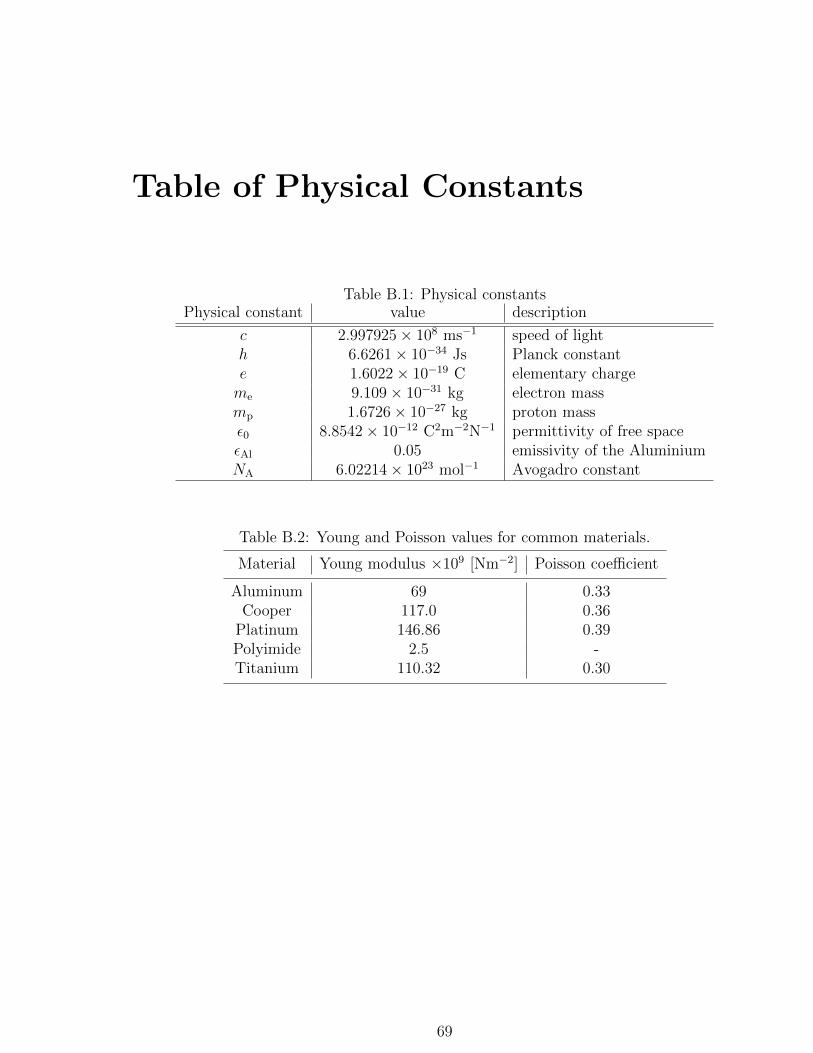
Table of Physical Constants
Table B.1: Physical constantsPhysical constant value description
c 2.997925× 10⁸ ms−1 speed of lighth 6.6261× 10⁻³⁴ Js Planck constante 1.6022× 10⁻¹⁹ C elementary chargeme 9.109× 10⁻³¹ kg electron massmp 1.6726× 10⁻²⁷ kg proton massε0 8.8542× 10⁻¹² C2m−2N−1 permittivity of free spaceεAl 0.05 emissivity of the AluminiumNA 6.02214× 10²³ mol−1 Avogadro constant
Table B.2: Young and Poisson values for common materials.
Material Young modulus ×109 [Nm−2] Poisson coefficient
Aluminum 69 0.33Cooper 117.0 0.36
Platinum 146.86 0.39Polyimide 2.5 -Titanium 110.32 0.30
69

70APPENDIX B. FORMATIONOF HYDROGENMOLECULAR BUBBLES ONMETAL SURFACES
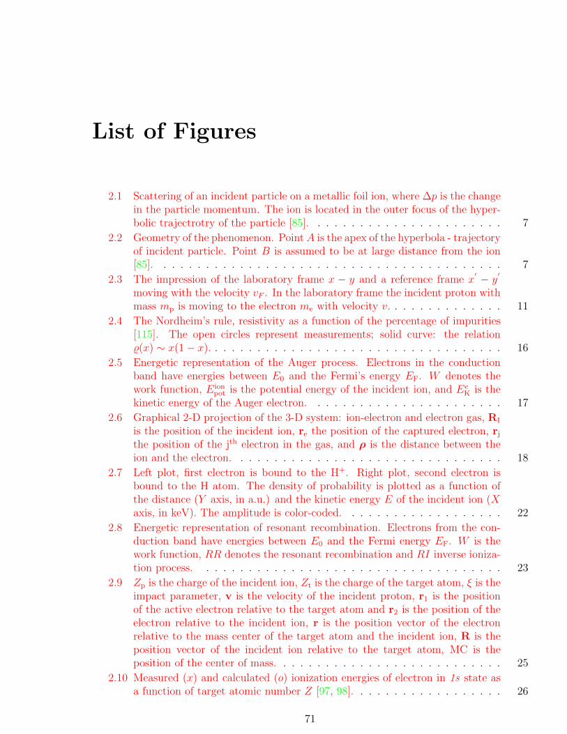
List of Figures
2.1 Scattering of an incident particle on a metallic foil ion, where ∆p is the changein the particle momentum. The ion is located in the outer focus of the hyper-bolic trajectrotry of the particle [85]. . . . . . . . . . . . . . . . . . . . . . . 7
2.2 Geometry of the phenomenon. Point A is the apex of the hyperbola - trajectoryof incident particle. Point B is assumed to be at large distance from the ion[85]. . . . . . . . . . . . . . . . . . . . . . . . . . . . . . . . . . . . . . . . . 7
2.3 The impression of the laboratory frame x − y and a reference frame x′ − y′
moving with the velocity vF . In the laboratory frame the incident proton withmass mp is moving to the electron me with velocity v. . . . . . . . . . . . . . 11
2.4 The Nordheim’s rule, resistivity as a function of the percentage of impurities[115]. The open circles represent measurements; solid curve: the relation%(x) ∼ x(1− x). . . . . . . . . . . . . . . . . . . . . . . . . . . . . . . . . . . 16
2.5 Energetic representation of the Auger process. Electrons in the conductionband have energies between E0 and the Fermi’s energy EF. W denotes thework function, Eion
pot is the potential energy of the incident ion, and EeK is the
kinetic energy of the Auger electron. . . . . . . . . . . . . . . . . . . . . . . 17
2.6 Graphical 2-D projection of the 3-D system: ion-electron and electron gas, RI
is the position of the incident ion, re the position of the captured electron, rj
the position of the jth electron in the gas, and ρ is the distance between theion and the electron. . . . . . . . . . . . . . . . . . . . . . . . . . . . . . . . 18
2.7 Left plot, first electron is bound to the H+. Right plot, second electron isbound to the H atom. The density of probability is plotted as a function ofthe distance (Y axis, in a.u.) and the kinetic energy E of the incident ion (Xaxis, in keV). The amplitude is color-coded. . . . . . . . . . . . . . . . . . . 22
2.8 Energetic representation of resonant recombination. Electrons from the con-duction band have energies between E0 and the Fermi energy EF. W is thework function, RR denotes the resonant recombination and RI inverse ioniza-tion process. . . . . . . . . . . . . . . . . . . . . . . . . . . . . . . . . . . . 23
2.9 Zp is the charge of the incident ion, Zt is the charge of the target atom, ξ is theimpact parameter, v is the velocity of the incident proton, r1 is the positionof the active electron relative to the target atom and r2 is the position of theelectron relative to the incident ion, r is the position vector of the electronrelative to the mass center of the target atom and the incident ion, R is theposition vector of the incident ion relative to the target atom, MC is theposition of the center of mass. . . . . . . . . . . . . . . . . . . . . . . . . . . 25
2.10 Measured (x) and calculated (o) ionization energies of electron in 1s state asa function of target atomic number Z [97, 98]. . . . . . . . . . . . . . . . . . 26
71
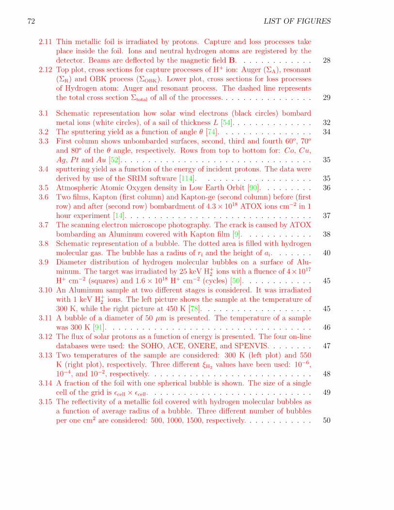
72 LIST OF FIGURES
2.11 Thin metallic foil is irradiated by protons. Capture and loss processes takeplace inside the foil. Ions and neutral hydrogen atoms are registered by thedetector. Beams are deflected by the magnetic field B. . . . . . . . . . . . . 28
2.12 Top plot, cross sections for capture processes of H+ ion: Auger (ΣA), resonant(ΣR) and OBK process (ΣOBK). Lower plot, cross sections for loss processesof Hydrogen atom: Auger and resonant process. The dashed line representsthe total cross section Σtotal of all of the processes. . . . . . . . . . . . . . . . 29
3.1 Schematic representation how solar wind electrons (black circles) bombardmetal ions (white circles), of a sail of thickness L [54]. . . . . . . . . . . . . . 32
3.2 The sputtering yield as a function of angle θ [74]. . . . . . . . . . . . . . . . 343.3 First column shows unbombarded surfaces, second, third and fourth 60o, 70o
and 80o of the θ angle, respectively. Rows from top to bottom for: Co, Cu,Ag, Pt and Au [52]. . . . . . . . . . . . . . . . . . . . . . . . . . . . . . . . . 35
3.4 sputtering yield as a function of the energy of incident protons. The data werederived by use of the SRIM software [114]. . . . . . . . . . . . . . . . . . . 35
3.5 Atmospheric Atomic Oxygen density in Low Earth Orbit [90]. . . . . . . . . 363.6 Two films, Kapton (first column) and Kapton-ge (second column) before (first
row) and after (second row) bombardment of 4.3× 10¹⁸ ATOX ions cm−2 in 1hour experiment [14]. . . . . . . . . . . . . . . . . . . . . . . . . . . . . . . . 37
3.7 The scanning electron microscope photography. The crack is caused by ATOXbombarding an Aluminum covered with Kapton film [9]. . . . . . . . . . . . 38
3.8 Schematic representation of a bubble. The dotted area is filled with hydrogenmolecular gas. The bubble has a radius of ri and the height of ai. . . . . . . 40
3.9 Diameter distribution of hydrogen molecular bubbles on a surface of Alu-minum. The target was irradiated by 25 keV H+
2 ions with a fluence of 4×10¹⁷
H+ cm−2 (squares) and 1.6× 10¹⁸ H+ cm−2 (cycles) [50]. . . . . . . . . . . . 453.10 An Aluminum sample at two different stages is considered. It was irradiated
with 1 keV H+2 ions. The left picture shows the sample at the temperature of
300 K, while the right picture at 450 K [78]. . . . . . . . . . . . . . . . . . . 453.11 A bubble of a diameter of 50 µm is presented. The temperature of a sample
was 300 K [91]. . . . . . . . . . . . . . . . . . . . . . . . . . . . . . . . . . . 463.12 The flux of solar protons as a function of energy is presented. The four on-line
databases were used: the SOHO, ACE, ONERE, and SPENVIS. . . . . . . . 473.13 Two temperatures of the sample are considered: 300 K (left plot) and 550
K (right plot), respectively. Three different ξH2 values have been used: 10−6,10−4, and 10−2, respectively. . . . . . . . . . . . . . . . . . . . . . . . . . . . 48
3.14 A fraction of the foil with one spherical bubble is shown. The size of a singlecell of the grid is εcell × εcell. . . . . . . . . . . . . . . . . . . . . . . . . . . . 49
3.15 The reflectivity of a metallic foil covered with hydrogen molecular bubbles asa function of average radius of a bubble. Three different number of bubblesper one cm2 are considered: 500, 1000, 1500, respectively. . . . . . . . . . . . 50
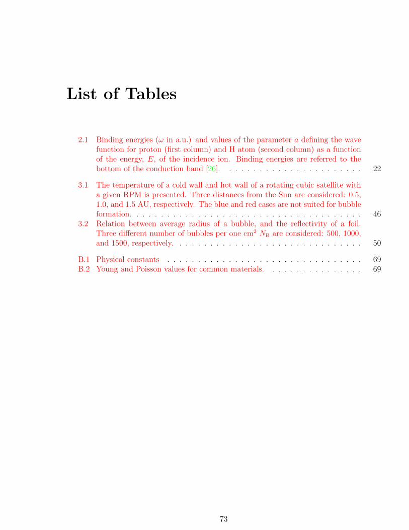
List of Tables
2.1 Binding energies (ω in a.u.) and values of the parameter a defining the wavefunction for proton (first column) and H atom (second column) as a functionof the energy, E, of the incidence ion. Binding energies are referred to thebottom of the conduction band [26]. . . . . . . . . . . . . . . . . . . . . . . 22
3.1 The temperature of a cold wall and hot wall of a rotating cubic satellite witha given RPM is presented. Three distances from the Sun are considered: 0.5,1.0, and 1.5 AU, respectively. The blue and red cases are not suited for bubbleformation. . . . . . . . . . . . . . . . . . . . . . . . . . . . . . . . . . . . . . 46
3.2 Relation between average radius of a bubble, and the reflectivity of a foil.Three different number of bubbles per one cm2 NB are considered: 500, 1000,and 1500, respectively. . . . . . . . . . . . . . . . . . . . . . . . . . . . . . . 50
B.1 Physical constants . . . . . . . . . . . . . . . . . . . . . . . . . . . . . . . . 69B.2 Young and Poisson values for common materials. . . . . . . . . . . . . . . . 69
73

74 LIST OF TABLES
Bibliography
[1] Abarenkov I. V., Physica Status Solidi B 50, 465 - 470, 1972.
[2] Abdullayeva M. K., Ayukhanov A. K., Shamsiyev U. B., Radiation Effects 19, 225-229,1973.
[3] Agnolan D., Study Overview of Solar Sail Demonstrator: Geosail, SCI-PA, 1, 1 - 54, 2007
[4] Alston S., Physical Review A 27, 2342-2357, 1983.
[5] Araminowicz J., Ma luszynska K., Przytu la M., Laboratorium Fizyki Jadrowej, PanstwoweWydawnictwo Naukowe, 1978.
[6] ASTM, E512-94(2010), Standard Particle for Combined, Simulated Space EnvironmentTesting of Thermal Control Materials with Electromagnetic and Particulate Radiation,2010
[7] Astrelin V. T., Burdakov A. V., Bykov P. V., Ivanov I. A., Ivanov A. A., Jongen Y.,Konstentinov S. G., Kudryavtsev A. M., Kuklin K. N., Mekler K. I., Polosatkin S. V.,Postupaev V. V., Rovenskikh A. F., Sinitskiy A. L., Zubairov E. R., Journal of NuclearMaterials 396, 43-48, 2009.
[8] Banks B. A., Atomic Oxygen Effects on Spacecraft Materials, NASA/TM-2003-212484,2003.
[9] Banks B. A., Scattered Atomic Oxygen Effects on Spacecraft Materials, Procedings ofthe 9th International Symposium on Materials in a Space Environment, 2003.
[10] Banyard K. E., Szuster B. J., Physical Review A 16, 129-132, 1977.
[11] Behrisch R., Ergebn. Exakt. Naturw. 35, 295, 1964.
[12] Belkic Dz., Gayet R., Salin A., Physics Reports 56, 279-369, 1979.
[13] Bid A., Bora A., Raychaudhuri A. K., Physical Review B 74, 035426-035434, 2006.
[14] Bitetti G., Marchetti M., Mileti S., Valente F., Scaglione S., Acta Astronautica 60,166-174, 2007.
[15] Bransden B. H., Cheshire I. M., Proceedings of the Physical Society 81, 820-832, 1963.
[16] Callaway J., Physical Review 97, 933-936, 1955.
[17] Carter G., Colligon J. S., Nobes M. J., Journal of Material Science 6, 115-117, 1971.
75
76 BIBLIOGRAPHY
[18] Canham L. T., Dyball M. R., Leong W. Y., Houlton M. R., Cullis A. G., Smith P. W.,Materials Science an Engineering: B 4, 41-45, 1989.
[19] Castaing R., Slodzian G., C. R. Acad. Sci. 255, 1893, 1962.
[20] Chew G. F., Physical Review 80, 196-202, 1950.
[21] Dachwald B., AIAA Conference, San Diego, California, 7 - 11 August 2005
[22] Daniels R. D., Journal of Applied Physics 42, 417-420, 1970.
[23] Das A., Melissions. A. C., Quantum Mechanics: A Modern Introduction, Gordon andBreach Science Publishers, 1990.
[24] Datta S. K., Crothers D. S. F., McCarroll R., Journal of Physics B: Atomic, Molecularand Optical Physics 23, 479-495, 1990.
[25] Decker F., Eichler J., Physical Review A 39, 1530-1533, 1989.
[26] Echenique P.M., Flores F., Ritchie R.H., Solid State Physics 43, 229-308, 1990.
[27] Echenique P.M., Flores F., Physical Review B 35, 8249-8251, 1987.
[28] ECSS-Q-ST-70-06C, Particle and UV Radiation Testing for Space Materials, 2008.
[29] ECSS-Q-ST-70-09C, Measurements of Thermo-Optical Properties Control Materials,2008.
[30] Farnsworth H. E., Schlier R. E., George T. H., Burger R. M., Journal of Applied Physics29, 1150-1162, 1958.
[31] Ford A. L., Reading J., F., Becker R. L., Physical Review A 23, 510-518, 1981.
[32] Garwin R. L., Jet Propulsion 28, 188-190, 1958.
[33] Geppert U., Biering B., Lura F., Block J., Straubel M., Rainhard R., Advances in SpaceResearch 48, 1695-1701, 2011.
[34] Ghosh M., Mandal C.R., Mukherjee S.C., Physical Review A 35, 2815-2820, 1987.
[35] Gravielle M.S., Miraglia J.E., Physical Review A 38, 5034-5037, 1988.
[36] Griffths D. J., Podstawy elektrodynamiki, Panstwowe Wydawnictwo Naukowe,Warszawa 2005.
[37] Grigorovici R., Denenyi A., Botila T., The number of free electrons in aluminium, 1961.
[38] Grossman E., Gouzman I., Nuclear Instruments and Methods in Physics Research B:Beam Interactions with Materials and Atoms 208, 48-57, 2003.
[39] Grossman E., Lifshitz Y., Wolan J. T., Moung Ch. K., Moung G. B., Journal of Space-craft and Rockets 36, 75-78, 1999.
BIBLIOGRAPHY 77
[40] Gudimenko Y., Ng R., Kleiman J. I., Iskanderova Z. A., Tennyson R. C., Hughes P.C., Milligan D., Grigorevski A., Shuiski M., Kiseleva L., Edwards D., Finckenor M.
”En-
hancement of Surface Durability of Space Materials and Structures in LEO Environment”,Procedings of the 9th International Symposium on Materials in a Space Environment,2003.
[41] Guinea F., Flores F., Echenique P.M., Physical Review B 25, 6109-6125, 1982.
[42] Habenicht S., Bolse W., Lieb K. P., Reimann K., Geyer U., Physical Review B 60,R2200-R2203, 1999.
[43] Hagstrum H. D., Physical Review 96, 336-365, 1954.
[44] Hartle J., B., Gravity An Introduction To Einstein’s General Relativity, Pearson Edu-cation,2003.
[45] Heltzel S., Semprimoschnig C. O. A., van Esbeek M. R. J., Journal of Spacecraft andRockets 46, 248-254, 2009.
[46] Herring C., Physical Review 57, 1169-1177, 1940.
[47] The HyperPhysics, Georgia State University, http://hyperphysics.phy.gsu.edu/hbase/quantum/fermi.html
[48] Izumi T., Itoh G., Materials Transactions 52, 130-134, 2011.
[49] Jackson J. D., Classical Electrodynamics, John Wiley & Sons, Inc., 1999.
[50] Kamada K., Sagara A., Kinoshita H., Takahashi H., Radiation Effects 103, 119-133,1986.
[51] Kaminsky M., Das S. K., Applied Physics Letters 21, 443-445, 1972.
[52] Karmakar P., Ghose D., Surface Science 554, L101-L106, 2004.
[53] Kezerashvili R. Ya., Matloff G. L., Advances in Space Research 44, 859-869, 2009.
[54] Kezerashvili R. Ya., Matloff G. L., Journal of British Interplanetary Society 60, 169-179,2007.
[55] Kuang Y. R., Physical Review A 44, 1613-1619, 1991.
[56] Kuang Y. R., Journal of Physics B: Atomic, Molecular and Optical Physics 24, 1645-1655, 1991.
[57] Landau L. D., Lifschitz M. J., Quantum Mechanics, Non-Relativistic Theory, 2003.
[58] Landau L. M., Lifschitz M. J., Theory of Elasticity, Pergamon Press, 1986.
[59] Lang K. R., Astrophysical Formulae: A Compedium for the Physicist and Astrophysicist,Spinger-Verlag, 1980.
[60] Lapicki G., Losonsky W., Physical Review A 15, 896-905, 1977.
[61] Lautrup B., Physics of Continuous Matter, 2nd Edition, Taylor & Francis Group, BacoRaton, Florida, USA, 2011.
78 BIBLIOGRAPHY
[62] Lieb H. J., Herzog R. F. K., Journal of Applied Physics 34, 2893-2897, 1963.
[63] Lin C. D., Soong S. C., Tunnell L. N., Physical Review A 17, 1646-1654, 1978.
[64] Lindhard J., Nielsen V., Scharff M., 1968, K. Danske Vidensk. Selsk. Math.-Fys. Meddr,36
[65] Lura F., Verhovtsva T., Yaremennko V. I., Telepnev V. D., Proceedings of the 7th
International Symposium on Materials in Space Environment, Toulouse, France, 119,1997
[66] Longair M. S., High Energy Astrophysics Vol 1: Particles, Photons and their Detection,Cambridge University Press, 1992.
[67] Lu G., Kaxiras E., Physics Review Letters 94, 155501-155505, 2005.
[68] Makeev M. A., Curno R., Barabasi A. L., Nuclear Instruments and Methods in PhysicsResearch Section B: Beam Interactions with Materials and Atoms 197, 185-227, 2002.
[69] Marco J., Remaury S., Tonon C., 11th International Symposium on Materials in a SpaceEnvironment, Aix-En-Provance, France, 2009.
[70] Martynenko Yu. V., Radiation Effects, 45, 93-101, 1979
[71] Mason Bruce, Homer L. Dodge Department of Physics and Astronomy, Quantum Physics- lectures
[72] McDonald M., McInnes C., Advances in Space Research 48, 1702-1716, 2011.
[73] McDonald R. J., Advances in Physics 19, 457-524, 1970.
[74] McCracken G. M., Reports on Progress in Physics 38, 241-327, 1975.
[75] Metzger H., Peisl J., Williams J., Journal of Physics F: Metal Physics 6, 2195-2207,1976.
[76] Minton T. K., Garton D., Advanced Series in Physical Chemistry 11, 420-489, 2001.
[77] Milacek L. H., Daniels R. D., Cooley J. A., Journal of Applied Physics 39, 2803-2816,1968.
[78] Milcius D., Pranevicius L. L., Templier C., J., Journal of Alloys and Compounds 398,203-207, 2005.
[79] Miraglia J. J., Physical Review A 30, 1721-1726, 1984.
[80] Montenbruck O., Gil E., Satellite Orbits: Models, Methods, Applications, 2005.
[81] Myers S. M., Baskes, M. I., Birnbaum, H. K., Corbett, J. W., Deleo, G. G., Estreicher,S. K., Haller, E. E., Jena, P., Johnson, N. M., Kirchheim, R., Pearton, S. J., Stavola, M.J., Review of Modern Physics 64, 559-617, 1992.
[82] Nahar S. N., Pradham A. K., Radiation Physics and Chemistry 70, 323-344, 2003.
BIBLIOGRAPHY 79
[83] Pauly N., Dubus A., Rosler M., Nuclear Instruments and Methods in Physics ResearchB: Beam Interactions with Materials and Atoms 193, 414 - 418, 2002.
[84] Penalba M., Arnau A., Echenique P.M., Nuclear Instruments and Methods in PhysicsResearch B: Beam Interactions with Materials and Atoms 48, 138-141, 1990.
[85] Podgorsak E. B., Radiation Physics for Medical Physicists, Springer - Verlag BerlinHildenberg, 2010.
[86] Pustowa low G. E., Fizyka Atomowa i Jadrowa, Panstwowe Wydawnictwo Naukowe,Warszawa 1972.
[87] Raisbeck G., Yiou F., Physical Review A 4, 1858-1868, 1971.
[88] Ree F. H., Bender C. F., Journal of Chemical Physics 71, 5362-5376, 1979.
[89] Ren X., Chu W., Li J., Su J., Qiao L., Materials Chemistry and Physics 107, 231-235,2008.
[90] Rooij A., Corrosion in Space - Encyclopedia of Aerospace Engineering, ESA-ESTEC,John Wiley & Sons Ltd., 2010.
[91] Rozenek P., International Journal of Hydrogen Energy 32, 2816-2823, 2007.
[92] Rosler M., Garcia de Abejo F.J., Physical Review B 54, 17158-17165, 1996.
[93] Romero M., Boscher D., ESA Workshop on Space Weather, ESA Space Environmentsand Effects Analysis Section (ESA TOS-EMA), ESTEC, Noordwijk, The Netherlands,1998.
[94] Rusponi S., Costantini G., Boragno C., Valbusa U., Physical Review Letters 81, 4184-4187, 1998.
[95] Schiff L. I., Quantum Mechanics, McGraw-Hill Book Company, Inc., 1955.
[96] Sharma A. K., Sridhara N., Advance in Space Research 50, 1411-1424, 2012
[97] Slater J. C., Physical Review 98, 1039-1045, 1955.
[98] Slater J. C., Quantum Theory of Atomic Structure, McGraw-Hill, 1960.
[99] Sigmund P., Physical Review 184, 383-416, 1969.
[100] Sols F., Flores F., Physical Review A 37, 1469-1475, 1988.
[101] Sols F., Flores F., Physical Review B 30, 4878-4880, 1984.
[102] Stopping-power and range tables for protons, National Institute of Standards and Tech-nology, http://physics.nist.gov/PhysRefData/Star/Text/PSTAR.html
[103] Szpikowski S., Podstawy Mechaniki Kwantowej, Wydawnictwo Uniwersytetu MariiCurie - Sk lodowskiej, 2006.
[104] Taute E., Physica Status Solidi (b) 142, 437-443, 1987.
80 BIBLIOGRAPHY
[105] Thomas G. J., Drotning W. D., Metallurgical Transactions A 14, 1545-1548, 1983.
[106] Vajo J. J., Doty R. E., Cirlin E. H., Journal of Vacuum Science & Technology A 14,2709-2721, 1996.
[107] Verner D. A., Ferland G. J., Astrophysical Journal Supplement 103, 467-473, 1996.
[108] Wigner E., Seitz F., Physical Review 43, 804-810, 1933.
[109] Winter T. G., Lin C. C., Physical Review A 10, 2141-2155, 1974.
[110] Winterbon B. K., Sigmund P., Sanders J. B., K. Denske Vidensk. Selsk., Math. -Fys.Meddr 37, 1970.
[111] Wittmaack K., Journal of Vacuum Science & Technology A 8, 2246-2251, 1990.
[112] Zhao X. H., Shen Z. G., Xing Y. S., Ma S. L., Journal of Physics D: Applied Physics34, 2308-2315, 2001.
[113] Ziegler J. F., Journal of Applied Physics 85, 1249-1273, 1999.
[114] Ziegler J. F., SRIM software, www.srim.org.
[115] Ziman J. M., Electrons and Phonons, Oxford at the Clarendon Press, 1960.
[116] Zimny R., Miskovic Z. L., Nedeljkovic N. N., Dedeljkovic Lj. D., Surface Science 255,135-156, 1991.