Lecture Notes in Mathematics 1980
199
Lecture Notes in Mathematics 1980 Editors: J.-M. Morel, Cachan F. Takens, Groningen B. Teissier, Paris
Transcript of Lecture Notes in Mathematics 1980

Lecture Notes in Mathematics 1980
Editors:J.-M. Morel, CachanF. Takens, GroningenB. Teissier, Paris

Krzysztof Bogdan · Tomasz ByczkowskiTadeusz Kulczycki · Michal RyznarRenming Song · Zoran Vondracek
Potential Analysis of StableProcesses and its Extensions
Volume Editors:Piotr GraczykAndrzej Stos
123
EditorsPiotr GraczykLAREMAUniversité d’Angers2 bd Lavoisier49045 [email protected]
Andrzej StosLaboratoire de MathématiquesUniversité Blaise PascalCampus Universitaire des Cézeaux63177 Aubiè[email protected]
Authors: see List of Contributors
ISBN: 978-3-642-02140-4 e-ISBN: 978-3-642-02141-1DOI: 10.1007/978-3-642-02141-1
Lecture Notes in Mathematics ISSN print edition: 0075-8434ISSN electronic edition: 1617-9692
Library of Congress Control Number: 2009928106
Mathematics Subject Classification (2000): 60J45, 60G52, 60J50, 60J75, 31B25, 31C05, 31C35, 31C25
c© Springer-Verlag Berlin Heidelberg 2009This work is subject to copyright. All rights are reserved, whether the whole or part of the material isconcerned, specifically the rights of translation, reprinting, reuse of illustrations, recitation, broadcasting,reproduction on microfilm or in any other way, and storage in data banks. Duplication of this publicationor parts thereof is permitted only under the provisions of the German Copyright Law of September 9,1965, in its current version, and permission for use must always be obtained from Springer. Violationsare liable to prosecution under the German Copyright Law.
The use of general descriptive names, registered names, trademarks, etc. in this publication does notimply, even in the absence of a specific statement, that such names are exempt from the relevant protectivelaws and regulations and therefore free for general use.
Cover design: SPi Publisher Services
Printed on acid-free paper
springer.com
Foreword
This monograph is devoted to the potential theory of stable stochasticprocesses and related topics, such as the subordinate Brownian motions (in-cluding the relativistic process) and Feynman–Kac semigroups generated bycertain Schrodinger operators.
The stable Levy processes and related stochastic processes play an impor-tant role in stochastic modelling in applied sciences, in particular in financialmathematics, and the theoretical motivation for the study of their fine prop-erties is also very strong. The potential theory of stable and related processesnaturally extends the theory established in the classical case of the Brownianmotion and the Laplace operator.
The foundations and general setting of probabilistic potential theory weregiven by G.A. Hunt [92](1957), R.M. Blumenthal and R.K. Getoor [23](1968),S.C. Port and J.C. Stone [130](1971). K.L. Chung and Z. Zhao [62](1995) havestudied the potential theory of the Brownian motion and related Schrodingeroperators. The present book focuses on classes of processes that contain theBrownian motion as a special case. A part of this volume may also be viewedas a probabilistic counterpart of the book of N.S. Landkof [117](1972).
The main part of Introduction that opens the book is a general presen-tation of fundamental objects of the potential theory of the isotropic stableLevy processes in comparison with those of the Brownian motion (presentedin a subsection). The introduction is accessible to a non-specialist. Also thechapters that follow should be of interest to a wider audience. A detaileddescription of the content of the book is given at the end of Chapter 1.
Some of the material of the book was presented by T. Byczkowski,T. Kulczycki, M. Ryznar and Z. Vondracek at the Workshop on Stochas-tic and Harmonic Analysis of Processes with Jumps held at Angers, France,May 2-9, 2006. The authors are grateful to the organizers and to the mainsupporters of the Workshop – the CNRS, the European Network of HarmonicAnalysis HARP and the University of Angers – for this opportunity, whichgave the incentive to write the monograph.
v

vi Foreword
The book was written while Z. Vondracek was visiting the Department ofMathematics of University of Illinois at Urbana-Champaign. He thanks thedepartment for the stimulating environment and hospitality. Thanks are alsodue to Andreas Kyprianou for several useful comments. The editors thankT. Luks for critical reading of some parts of the manuscript and for some ofthe figures illustrating the text.

Contents
1 Introduction . . . . . . . . . . . . . . . . . . . . . . . . . . . . . . . . . . . . . . . . . . . . . . . . . . . . . . . . . . . . 11.1 Bases of Potential Theory of Stable Processes. . . . . . . . . . . . . . . . . . 1
1.1.1 Classical Potential Theory . . . . . . . . . . . . . . . . . . . . . . . . . . . . . . 21.1.2 Potential Theory of the Riesz Kernel . . . . . . . . . . . . . . . . . . 71.1.3 Green Function and Poisson Kernel of Δα/2 . . . . . . . . . . 141.1.4 Subordinate Brownian Motions . . . . . . . . . . . . . . . . . . . . . . . . 22
1.2 Outline of the Book . . . . . . . . . . . . . . . . . . . . . . . . . . . . . . . . . . . . . . . . . . . . . . 23
2 Boundary Potential Theory for SchrodingerOperators Based on Fractional Laplacian . . . . . . . . . . . . . . . . . . . . . . . 25K. Bogdan and T. Byczkowski2.1 Introduction . . . . . . . . . . . . . . . . . . . . . . . . . . . . . . . . . . . . . . . . . . . . . . . . . . . . . . . 252.2 Boundary Harnack Principle . . . . . . . . . . . . . . . . . . . . . . . . . . . . . . . . . . . . . 262.3 Approximate Factorization of Green Function . . . . . . . . . . . . . . . . . 352.4 Schrodinger Operator and Conditional Gauge Theorem . . . . . . . 37
3 Nontangential Convergence for α-harmonicFunctions . . . . . . . . . . . . . . . . . . . . . . . . . . . . . . . . . . . . . . . . . . . . . . . . . . . . . . . . . . . . . . . . 57M. Ryznar3.1 Introduction . . . . . . . . . . . . . . . . . . . . . . . . . . . . . . . . . . . . . . . . . . . . . . . . . . . . . . . 573.2 Basic Definitions and Properties . . . . . . . . . . . . . . . . . . . . . . . . . . . . . . . . 603.3 Relative Fatou Theorem for α-Harmonic Functions. . . . . . . . . . . . 623.4 Extensions to Other Processes . . . . . . . . . . . . . . . . . . . . . . . . . . . . . . . . . . . 70
4 Eigenvalues and Eigenfunctions for StableProcesses . . . . . . . . . . . . . . . . . . . . . . . . . . . . . . . . . . . . . . . . . . . . . . . . . . . . . . . . . . . . . . . . 73T. Kulczycki4.1 Introduction . . . . . . . . . . . . . . . . . . . . . . . . . . . . . . . . . . . . . . . . . . . . . . . . . . . . . . . 734.2 Intrinsic Ultracontractivity (IU) . . . . . . . . . . . . . . . . . . . . . . . . . . . . . . . . . 764.3 Steklov Problem . . . . . . . . . . . . . . . . . . . . . . . . . . . . . . . . . . . . . . . . . . . . . . . . . . 784.4 Eigenvalue Estimates . . . . . . . . . . . . . . . . . . . . . . . . . . . . . . . . . . . . . . . . . . . . . 814.5 Generalized Isoperimetric Inequalities . . . . . . . . . . . . . . . . . . . . . . . . . . 82
vii

viii Contents
5 Potential Theory of Subordinate Brownian Motion . . . . . . . . . . 87R. Song and Z. Vondracek5.1 Introduction . . . . . . . . . . . . . . . . . . . . . . . . . . . . . . . . . . . . . . . . . . . . . . . . . . . . . . . 875.2 Subordinators . . . . . . . . . . . . . . . . . . . . . . . . . . . . . . . . . . . . . . . . . . . . . . . . . . . . . 89
5.2.1 Special Subordinators and CompleteBernstein Functions . . . . . . . . . . . . . . . . . . . . . . . . . . . . . . . . . . . . . 89
5.2.2 Examples of Subordinators . . . . . . . . . . . . . . . . . . . . . . . . . . . . . 965.2.3 Asymptotic Behavior of the Potential,
Levy and Transition Densities . . . . . . . . . . . . . . . . . . . . . . . . . . 1025.3 Subordinate Brownian Motion . . . . . . . . . . . . . . . . . . . . . . . . . . . . . . . . . . . 110
5.3.1 Definitions and Technical Lemma . . . . . . . . . . . . . . . . . . . . . . 1105.3.2 Asymptotic Behavior of the Green Function . . . . . . . . . . 1155.3.3 Asymptotic Behavior of the Jumping Function . . . . . . . 1225.3.4 Transition Densities of Symmetric
Geometric Stable Processes . . . . . . . . . . . . . . . . . . . . . . . . . . . . . 1295.4 Harnack Inequality for Subordinate Brownian Motion . . . . . . . . 131
5.4.1 Capacity and Exit Time Estimatesfor Some Symmetric Levy Processes . . . . . . . . . . . . . . . . . . . 131
5.4.2 Krylov-Safonov-type Estimate. . . . . . . . . . . . . . . . . . . . . . . . . . 1355.4.3 Proof of Harnack Inequality . . . . . . . . . . . . . . . . . . . . . . . . . . . . 141
5.5 Subordinate Killed Brownian Motion . . . . . . . . . . . . . . . . . . . . . . . . . . . 1485.5.1 Definitions . . . . . . . . . . . . . . . . . . . . . . . . . . . . . . . . . . . . . . . . . . . . . . . 1485.5.2 Representation of Excessive and Harmonic
Functions of Subordinate Process . . . . . . . . . . . . . . . . . . . . . . 1505.5.3 Harnack Inequality for Subordinate Process . . . . . . . . . . 1585.5.4 Martin Boundary of Subordinate Process . . . . . . . . . . . . . 1615.5.5 Boundary Harnack Principle for Subordinate
Process . . . . . . . . . . . . . . . . . . . . . . . . . . . . . . . . . . . . . . . . . . . . . . . . . . . 1675.5.6 Sharp Bounds for the Green Function
and the Jumping Function of Subordinate Process . . . 171
Bibliography . . . . . . . . . . . . . . . . . . . . . . . . . . . . . . . . . . . . . . . . . . . . . . . . . . . . . . . . . . . . . . . . 177
Index . . . . . . . . . . . . . . . . . . . . . . . . . . . . . . . . . . . . . . . . . . . . . . . . . . . . . . . . . . . . . . . . . . . . . . . . . 185

List of Contributors
Krzysztof Bogdan Institute of Mathematics and Computer ScienceWroc�law University of Technology, ul. Wybrzeze Wyspianskiego 27, 50-370Wroc�law, Poland. [email protected] research of this author was partially supported by grant MNiI 1 P03A 026 29.
Tomasz Byczkowski Institute of Mathematics and Computer Science,Wroc�law University of Technology, ul. Wybrzeze Wyspianskiego 27, 50-370Wroc�law, Poland. [email protected] research of this author was partially supported by KBN Grant 1 P03A 020
28 and RTN Harmonic Analysis and Related Problems, contract HPRN-CT-2001-
00273-HARP.
Tadeusz Kulczycki Institute of Mathematics, Polish Academy ofSciences, ul. Kopernika 18, 51-617 Wroc�law, Poland and Institute ofMathematics and Computer Science, Wroc�law University of Tech-nology, ul. Wybrzeze Wyspianskiego 27, 50-370 Wroc�law, [email protected] research of this author was partially supported by KBN Grant 1 P03A 020
28 and RTN Harmonic Analysis and Related Problems, contract HPRN-CT-2001-
00273-HARP.
Micha�l Ryznar Institute of Mathematics and Computer Science, Wroc�lawUniversity of Technology, ul. Wybrzeze Wyspianskiego 27, 50-370 Wroc�law,Poland. [email protected] research of this author was partially supported by KBN Grant 1 P03A 020
28 and RTN Harmonic Analysis and Related Problems, contract HPRN-CT-2001-
00273-HARP.
Renming Song Department of Mathematics, University of Illinois,Urbana, IL 61801. [email protected] research of this author is supported in part by a joint US-Croatia grant INT
0302167.
Zoran Vondracek Department of Mathematics, University of Zagreb,Zagreb, Croatia. [email protected]
The research of this author is supported in part by MZOS grant 037-0372790-2801
of the Republic of Croatia.
ix

Chapter 1
Introduction
1.1 Bases of Potential Theory of Stable Processes
In 1957, G. A. Hunt introduced and developed the potential theory of Markovprocesses in his fundamental treatise [92]. Hunt’s theory is essentially basedon the fact that the integral of the transition probability of a Markov processdefines a potential kernel:
U(x, y) =∫ ∞
0
p(t, x, y)dt .
One of the important topics in the theory is the study of multiplicativefunctionals of the Markov process, corresponding either to Schrodinger per-turbations of the generator of the process, or to killing the process atcertain stopping times. Among the most influential treatises on this subjectare the monographs [23] by R. M. Blumenthal and R. K. Getoor, [60] byK. L. Chung, [22] by W. Hansen and J. Bliedtner, and [62] by K. L. Chungand Z. Zhao.
Harmonic functions of a strong Markov process are defined by the meanvalue property with respect to the distribution of the process stopped at thefirst exit time of a domain. An important case of such a function is thepotential of a measure not charging the domain, thus yielding no “sources”to change the expected occupation time of the process.
To produce specific results, however, the general framework of Hunt’s the-ory requires precise information on the asymptotics of the potential kernel ofthe given Markov process. For instance, the process of the Brownian motionin R
3 is generated by the Laplacian, Δ, and yields the Newtonian kernel,x �→ c|x − y|−1. Here y is the source or pole of the kernel. When x0 is fixedand |y| → ∞, we have that, regardless of x, |x− y|−1/|x0 − y|−1 → 1, whicheventually leads to the conclusion that nonnegative functions harmonic onthe whole of R
3 must be constant.Explicit formulas for the potential kernel are rare. Even the Brownian
motion killed when first exiting a subdomain of Rd in general leads to a
K. Bogdan et al., Potential Analysis of Stable Processes and its Extensions,Lecture Notes in Mathematics 1980, DOI 10.1007/978-3-642-02141-1 1,c© Springer-Verlag Berlin Heidelberg 2009
1

2 1 Introduction
transition density and potential kernel which are not given by closed-formformulas, and may be even difficult to estimate.
A primary example of a jump process is the isotropic α-stable Levy processin R
d, whose potential kernel is the M. Riesz’ kernel. The analytic theory ofthe Riesz kernel, the fractional Laplacian Δα/2, and the corresponding α-harmonic functions had been well established for a long time (see [133] and[117]). However, until recently little was known about the boundary behaviorof α-harmonic functions on sub-domains of R
d.We begin the book by presenting some of the basic objects and results of
the classical (Newtonian) potential theory (α = 2), and Riesz potential the-ory (0 < α < 2). We have already mentioned the well known but remarkablefact that the (Newtonian) potential theory of the Laplacian can be inter-preted and developed by means of the Brownian motion ([71]). An analogousrelationship holds for the (Riesz) potential theory of the fractional Laplacianand the isotropic α-stable Levy process. We pursue this relationship in thefollowing sections. We like to remark that Δα/2 is a primary example of anonlocal pseudo differential operator ([97]) and we hope that a part of ourdiscussion will extend to other nonlocal operators. Apart from its significancein mathematics, the fractional Laplacian appears in theoretical physics in theconnection to the problem of stability of the matter [118]. Namely, the oper-ator I − (I −Δ)1/2 corresponds to the kinetic energy of a relativistic particleand Δ1/2 can be regarded as an approximation to I − (I −Δ)1/2, see, e.g.,[45], [134].
In what follows, functions and sets are assumed to be Borel measurable.We will write f ≈ g to indicate that f and g are comparable, i.e. there is aconstant c (a positive real number independent of x), such that c−1f(x) �g(x) � cf(x). Values of constants may change from place to place, for instancef(x) � (2c + 1)g(x) = cg(x) should not alarm the reader.
1.1.1 Classical Potential Theory
We consider the Gaussian kernel,
gt(x) =1
(4πt)d/2e−|x|2/4t , x ∈ R
d , t > 0 . (1.1)
It is well known that {gt, t � 0} form a convolution semigroup: gs∗gt = gs+t,where s, t > 0. This property is at the heart of the classical potential theory.Complicating the notation slightly, we define transition probability
g(s, x, t, A) =∫
A−x
gt−s(y)dy , s < t , x ∈ Rd , A ⊂ R
d . (1.2)

1 Introduction 3
The semigroup property of {gt} is equivalent to the following Chapman-Kolmogorov equation∫
Rd
g(s, x, u, dz)g(u, z, t, A) = g(s, x, t, A) , s < u < t , x ∈ Rd , A ⊂ R
d .
If d � 3 then we define and calculate the Newtonian kernel,
N(x) =∫ ∞
0
gt(x)dt = Ad,2|x|2−d , x ∈ Rd .
Here and below
Ad,γ = Γ((d− γ)/2)/(2γπd/2|Γ(γ/2)|) . (1.3)
The semigroup property yields that N ∗ gs(x) =∫∞
sgt(x)dt � N(x). Recall
that a function h ∈ C2(D) is called harmonic in an open set D ⊆ Rd if it
satisfies Laplace’s equation,
Δh(x) =d∑
i=1
∂2h(x)∂x2
i
= 0 , x ∈ D . (1.4)
It is well known that N is harmonic on Rd \ {0}. Let B(a, r) = {x ∈ R
d :|x−a| < r}, where a ∈ R
d, r > 0. We also let Br = B(0, r), B = B1 = B(0, 1).The Poisson kernel of B(a, r) is
P (x, z) =Γ(d/2)2πd/2r
r2 − |x− a|2|x− z|d , x ∈ B(a, r) , z ∈ ∂B(a, r) . (1.5)
It is well known that if h is harmonic in an open set containing the closureof B(a, r) then
h(x) =∫
∂B(a,r)
h(z)P (x, z)σ(dz) , x ∈ B(a, r) . (1.6)
Here σ denotes the (d− 1)-dimensional Haussdorff measure on ∂B(a, r). Welike to note that P (x, z) is positive and continuous on B(a, r)×∂B(a, r), andhas the following properties:
∫∂B(a,r)
P (x, z)σ(dz) = 1 , x ∈ B(a, r) , (1.7)
limx→w
∫∂B(a,r)\B(w,δ)
P (x, z)σ(dz) = 0 , w ∈ ∂B(a, r) , δ > 0 . (1.8)

4 1 Introduction
It is also well known that for every z ∈ ∂B(a, r), P (·, z) is harmonic in B(a, r),a property resembling Chapman-Kolmogorov equation if we consider (1.6) forh(x) = P (x, z0). Consequently, if f ∈ C(∂B(a, r)), then the Poisson integral,
P [f ](x) =∫
∂B(a,r)
P (x, z) f(z)σ(dz) , x ∈ B(a, r) , (1.9)
solves the Dirichlet problem for B(a, r) and f . Namely, P [f ] extends tothe unique continuous function on B(a, r) ∪ ∂B(a, r), which is harmonic inB(a, r), and coincides with f on ∂B(a, r), see (1.8). In particular, P [1] ≡ 1,compare (1.7).
An analogous Martin representation is valid for every nonnegative h har-monic on B(a, r),
h(x) = P [μ](x) :=∫
∂B(a,r)
P (x, z)μ(dz) , x ∈ B(a, r) . (1.10)
Here μ � 0 is a unique nonnegative measure on ∂B(a, r). We like to note thatappropriate sections of P [μ] weakly converge to μ ([107]), which reminds usthat in general the boundary values of harmonic functions require handlingwith care.
By (1.5) we have that P (x1, z) � (1 + s/r)d(1− s/r)−dP (x2, z) if x1, x2 ∈B(a, s), s < r, z ∈ ∂B(a, r). As a direct application of (1.10) we obtain thefollowing Harnack inequality,
c−1h(x1) � h(x2) � c h(x1) , x1, x2 ∈ B(a, s) , (1.11)
provided h is nonnegative harmonic. We see that h is nearly constant (i.e.comparable with 1) on B(a, s) for s < r. If D is connected, then consideringfinite coverings of compact K ⊂ D by overlapping chains of balls, we seethat nonnegative functions h harmonic on D are nearly constant on K, seeFigure 1.1.
K
D
Fig. 1.1 Harnack chain

1 Introduction 5
Despite its general importance, Harnack inequality is less useful at theboundary of the domain because the corresponding constant gets inflated forpoints close to the boundary. In fact, nonnegative harmonic functions presenta complicated array of asymptotic behaviors at the boundary, see (1.5). Tostudy the asymptotics, we first concentrate on nonnegative harmonic functionvanishing at a part of the boundary.
The Boundary Harnack Principle (BHP) for classical harmonic functionsdelicately depends on the geometric regularity of the domain. To simplifyour discussion we will consider the following Lipschitz condition. Let d � 2.Recall that Γ : R
d−1 → R is called Lipschitz if there is λ <∞ such that
|Γ(y)− Γ(z)| � λ|z − y| , y, z ∈ Rd−1 . (1.12)
We define (special Lipschitz domain)
DΓ = {x = (x1, . . . , xd) ∈ Rd : xd > Γ(x1, . . . , xd−1)} . (1.13)
A nonempty open D ⊆ Rd is called a Lipschitz domain if for every z ∈ ∂D
there exist r > 0, a Lipschitz function Γ : Rd−1 → R, and an isometry T of
Rd, such that D∩B(z, r) = T (DΓ)∩B(z, r), that is, if D is locally isometric
with a set “above” the graph of a Lipschitz function.
Theorem 1.1 (Boundary Harnack Principle). Let D be a connectedLipschitz domain. Let U ⊂ R
d be open and let K ⊂ U be compact. Thereexists C < ∞ such that for every (nonzero) functions u, v � 0, which areharmonic in D and vanish continuously on Dc ∩ U , we have
C−1 u(y)v(y)
� u(x)v(x)
� Cu(y)v(y)
, x, y ∈ K ∩D . (1.14)
Thus, the ratio u/v is nearly constant on D ∩ K. Furthermore, under theabove assumptions,
limx→z
u(x)v(x)
exists as x→ z ∈ ∂D ∩K , (1.15)
see Figure 1.2.The theorem is crucial in the study of asymptotics and structure of general
nonnegative harmonic functions in Lipschitz domains. The proof of BHP forclassical harmonic functions in Lipschitz domains was independently givenby B. Dahlberg(1977), A. Ancona(1978) and J.-M. Wu(1978), and (1.15) waspublished by D. Jerison and C. Kenig in 1982.
We now return to {gt}, and the resulting transition probability g. ByWiener’s theorem there are probability measures P x, x ∈ R
d, on the spaceof all continuous functions (paths) [0,∞) t �→ X(t) ∈ R
d, such thatP x0(X(0) = x0) = 1 and P x0(Xt ∈ A|Xs = x) = g(s, x, t, A) = P x(Xt−s ∈

6 1 Introduction
Fig. 1.2 The setup ofBHP
K
U
D
y
x
A), for x0, x ∈ Rd, 0 � s < t, A ⊂ R
d. Recall that the construction of thedistribution of the process from a transition probability on this path spacerequires certain continuity properties of the transition probability in time.Here we have limt→0 gt(x)/t = 0 (x �= 0), which eventually allows the pathsto be continuous by Kolmogorov’s test or by Kinney-Dynkin theorem, see[135]. Thus, Xt is continuous. Denote X = (Xt) = (X1
t , . . . , Xdt ), and let Ex
be the integration with respect to P x. We have E0Xit = 0, E0(Xi
t)2 = 2t.
Thus, Xt = B2t, where Bt is the usual Brownian motion with variance ofeach coordinate equal to t.
By the construction, Exf(Xt) =∫
Rd f(y)g(0, x, t, dy) =∫
Rd f(y)gt(y −x)dy for x ∈ R
d, t > 0, and nonnegative or integrable f . For a (Borel) setA ⊂ R
d by Fubini-Tonelli theorem,
Ex
∫ ∞
0
1A(Xt)dt =∫
A
N(y − x)dy , x ∈ Rd .
Therefore N(·−x) may be interpreted as the density function of (the measureof) the expected occupation time of the process, when started at x.
So far we have only considered X evaluated at constant (deterministic)times t. For an open D ⊆ R
d we now define the first exit time from D,
τD = inf{t > 0 : Xt �∈ D} .
By the usual convention, inf ∅ = ∞. τD is a Markov (stopping) time. Afunction h defined and Borel measurable on R
d is harmonic on D if for everyopen bounded set U such that U ⊆ D (denoted U ⊂⊂ D) we have
h(x) = Exh(XτU) , x ∈ U . (1.16)
1 Introduction 7
We assume here the absolute convergence of the integral. Since the P x-distribution of XτB(x,r) is the normalized surface measure on the sphere∂B(x, r), the equality (1.16) reads as follows:
h(x) =∫
∂B(x,r)
h(y)P (0, y − x)σ(dy) ,
if x ∈ U = B(a, r), see (1.5) and (1.6). Thus, (1.16) agrees with the classicaldefinition of harmonicity.
The above definitions may and will be extended below to other strongMarkov processes, and (1.16) may be referred to as the “averaging property”or “mean value property”.
We should note that (for the Brownian motion) the values of h on Dc areirrelevant in (1.16) because XτU
∈ ∂U ⊂ D in (1.16). For the isotropic stableLevy process, which we will discuss below, the support of the distributionof the process stopped at the first exit time of a domain is typically thewhole complement of the domain. Indeed, as time (t) advances, the pathsof the process may leave the domain either by continuously approaching theboundary or by a direct jump to the complement of the domain. In particular,a harmonic function should generally be defined on the whole of R
d. It is ofconsiderable importance to classify nonnegative harmonic functions of theprocess according to these two scenarios, see the concluding remarks in [38].
To indicate the role of the strong Markov property, we consider a nonneg-ative function h on Dc and we let h(x) = Exh(XτD
), x ∈ D. We will regardh on Dc as the boundary/external values of h, as appropriate for generalprocesses with jumps. It will be convenient to write h(x) for h(x) if x ∈ Dc.Let x ∈ U ⊂⊂ D. We have
Exh(XτU) = ExEXτU h(XτD
) = Exh(XτD) = h(x) .
In particular we see that h is harmonic on U . The above essentially also provesthat {h(XτU
)} is a martingale ordered by the inclusion of (open relativelycompact) subsets U of D, with respect to every P x, x ∈ D. Closability ofsuch martingales is of some interest in this theory [27, 38], and relates tothe existence of boundary values of harmonic functions. For instance themartingales given by Poisson integrals (1.10) are not closable for singularmeasures μ on ∂B(a, r).
1.1.2 Potential Theory of the Riesz Kernel
We will introduce the principal object of this book, namely the isotropic(rotation invariant) α-stable Levy process. We will construct the transitiondensity of the process by using convolution semigroups of measures. For a
8 1 Introduction
measure γ on Rd, we let |γ| denote its total mass. For a function f we let
γ(f) =∫
fdγ, whenever the integral makes sense. When |γ| < ∞ and n =1, 2, . . . we let γn = γ ∗ . . . ∗ γ (n times) denote the n-fold convolution of γwith itself:
γn(f) =∫
f(x1 + x2 + · · ·+ xn)γ(dx1)γ(dx2) . . . γ(dxn) .
We also let γ0 = δ0, the evaluation at 0. If γ is finite on Rd then we define
P γt = exp t(γ − |γ|δ0) :=
∞∑n=0
tn (γ − |γ|δ0)n
n!(1.17)
= (exp −t|γ|δ0) ∗ exp tγ = e−t|γ|∞∑
n=0
tnγn
n!, t ∈ R . (1.18)
By (1.18) each P γt is a probability measure, provided γ � 0 and t � 0, which
we will assume in what follows. By (1.17), P γt form a convolution semigroup,
P γt ∗ P γ
s = P γs+t , s, t � 0 .
Furthermore, for two such measures γ1, γ2, we have
P γ1t ∗ P γ2
t = P γ1+γ2t , t > 0 .
By (1.17),limt→0
(P γt − δ0)/t = γ − |γ|δ0 . (1.19)
In the following discussion for simplicity we will also assume that γ hasbounded support and that γ is symmetric: γ(−A) = γ(A), A ⊂ R
d. Thereader may want to verify that
∫Rd
|y|2P γt (dy) = t
∫Rd
|y|2γ(dy) < ∞ , t � 0 . (1.20)
As a hint we note that only the third term in (1.17) contributes to (1.20).In particular,
P γt (B(0, R)c) � t
∫Rd
|y|2γ(dy)/R2 → 0 as R →∞ . (1.21)
We defineν(B) = Ad,−α
∫B
|z|−d−αdz , B ⊂ Rd . (1.22)

1 Introduction 9
It is a Levy measure, i.e. a nonnegative measure on Rd \ {0} satisfying
∫Rd
min(|y|2, 1) ν(dy) <∞ . (1.23)
We also note that ν is symmetric. We consider the following operator, thefractional Laplacian,
Δα/2u(x) = Ad,−α limε→0+
∫{y∈Rd: |y−x|>ε}
u(y)− u(x)|y − x|d+α
dy . (1.24)
The limit exists if, say, u is C2 near x and bounded on Rd. The claim follows
from Taylor expansion of u at x, with remainder of order two, and by thesymmetry of ν. We like to note that A = Δα/2 satisfies the positive maximumprinciple: for every ϕ ∈ C∞
c (Rd)
supy∈Rd
ϕ(y) = ϕ(x) � 0 implies Aϕ(x) � 0 .
The most general operators on C∞c (Rd) which have this property are of the
form
Aϕ(x) =d∑
i,j=1
aij(x)DxiDxj
ϕ(x) + b(x)∇ϕ(x) + q(x)ϕ(x)
+∫
Rd
(ϕ(x + y)− ϕ(x)− y∇ϕ(x) 1|y|<1
)μ(x, dy) . (1.25)
Here y∇ϕ is the scalar product of y and the gradient of ϕ, and for everyx, a(x) = (aij(x))n
i,j=1 is a real nonnegative definite symmetric matrix, thevector b(x) = (bi(x))d
i=1 has real coordinates, q(x) � 0, and μ(x, ·) is a Levymeasure. The description is due to Courrege, see [90, Proposition 2.10], [151,Chapter 2] or [97, Chapter 4.5]. For translation invariant operators of thistype, a, b, q, and μ are independent of x. For Δα/2 we further have a = 0,b = 0, q = 0 and μ = ν.
For r > 0 and a function ϕ on Rd we consider its dilation ϕr(y) = ϕ(y/r),
and we note that ν(ϕr) = r−αν(ϕ). In particular, ν is homogeneous: ν(rB) =r−αν(B), B ⊂ R
d. Similarly, if ϕ ∈ C∞c (Rd), then Δα/2(ϕr) = r−α(Δα/2ϕ)r.
We will consider approximations of ν and Δα/2 suggested by (1.24). For0 < δ � ε �∞ we define measures νδ,ε(f) =
∫δ≤|y|<ε
f(y)ν(dy). We have
Pνδ,∞t − P
νε,∞t = P
νε,∞t ∗
(P
νδ,ε
t − δ0
). (1.26)
When ε → 0, the above converges (uniformly in δ) to 0 on each C∞c function
with compact support. This claim follows from Taylor expansion with the

10 1 Introduction
quadratic remainder, (1.20) applied to γ = νδ,ε, (1.23), and the fact thatP
νε,∞t are probabilities, hence uniformly finite.If φ is a bounded continuous function on R
d, η > 0, and 0 < R < ∞, thenthere is ϕ ∈ C∞
c such that |φ− ϕ| < η on B(0, R). We have
|(P
νδ,∞t − P
νε,∞t
)(φ)| � |
(P
νδ,∞t − P
νε,∞t
)(ϕ)|+ 2η
+[P
ν1,∞t ∗ P
νδ,1t (B(0, R)c)
+ Pν1,∞t ∗ P
νε,1t (B(0, R)c)
]sup |φ− ϕ| .
By inspecting (1.21) we see that the measures Pνε,∞t weakly converge to a
probability measure, say Pt, as ε → 0, and so {Pt, t � 0} is a convolutionsemigroup, too. We also note that Pt/t weakly converges to ν on (closedsubsets of) R
d \ {0}. This follows from the approximation of Pt by Pνε,∞t ,
and (1.19).The Fourier transform of P ε
t is easily calculated from (1.17),
Pνε,∞t (u) =
∫Rd
eiuyPνε,∞t (dy) = exp
(t
∫Rd
(eiuy − 1)νε,∞(dy))
, u ∈ Rd ,
(1.27)hence Pt(u) = exp(tΦ(u)), where
Φ(u) =∫
Rd
(eiuy − 1− iuy1B(0,1)(y)
)ν(dy)
=∫
Rd
(cos(uy)−1) ν(dy) = − π
2 sin πα2 Γ(1+α)
∫|ξ|=1
|uξ|ασ(dξ) = −c|u|α.
(1.28)
In fact, c = 1 here, and Φ(u) = −|u|α as we shall see momentarily.For t > 0, the measures Pt have rapidly decreasing Fourier transform hence
they are absolutely continuous with bounded smooth densities, pt(x), givenby the Fourier inversion formula:
pt(x) = (2π)−d
∫Rd
eixu e−t|u|α du . (1.29)
Explicit formulas for the pt do not exist except for α = 1,
pt(x) =Γ(
d+12
)π
d+12
t
(t2 + |x|2) d+12
,
and α = 2, which corresponds to the Brownian motion and is excluded fromour present considerations. Clearly, ps ∗pt(x) = ps+t(x), s, t > 0. From (1.28)we obtain the scaling property:
pt(x) = t−d/αp1(t−1/αx) , x ∈ Rd , t > 0 . (1.30)
1 Introduction 11
In particular,pt(x) � ct−d/α . (1.31)
We define the potential kernel (M. Riesz kernel) of the convolution semigroupof functions {pt}:
Kα(x) =∫ ∞
0
pt(x)dt , x ∈ Rd . (1.32)
When d > α, we have that Kα(x) is finite for x �= 0, see (1.31). By (1.30),
Kα(x) = Ad,α|x|α−d . (1.33)
The explicit constant here and in (1.28) may be obtained by a calculationinvolving Bessel functions, but it is easier to employ the Laplace transform tothis end (see below). Since Kα ≡ ∞ if α � d, and cumbersome modificationsare needed in this case, the dimension d = 1 is explicitly excluded fromour considerations. We refer to [41] for more information and references onthe case d = 1. Unless stated otherwise in the remainder of this chapter weassume that d � 2.
We construct the standard isotropic α-stable Levy process (Yt, Px) in R
d
by specifying the following density function of its transition probability:
p(s, x, t, y) := pt−s(y − x) , x, y ∈ Rd , s < t ,
and stipulating that P x(Y (0) = x) = 1. This is completely analogous to theconstruction of the Brownian motion, except for the fact that the distributionof the process is eventually concentrated on right continuous paths with leftlimits (rather than on continuous paths). The latter follows from the Kinney-Dynkin theorem and the fact that Pt/t converges to ν �= 0. In fact Yt hasdiscontinuities of the first kind, that is jumps (by z), occurring in time (t) withintensity ν(dz)dt ([135]), see Figure 1.3. The term standard above involvescertain technical measure-theoretic and topological assumptions, involvingthe right continuity and left-limitedness of the paths t �→ Yt as mentionedabove, and the so called quasi-left continuity, see, e.g., [18], [23] for moredetails. The process (Yt, P
x) is Markov on Rd with transition probabilities
P x0(Yt ∈ A|Ys = x) =∫
Ap(s, x, t, y)dy, for x0, x ∈ R
d, 0 � s < t, A ⊂ Rd;
and initial distribution is specified by P x0(Y (0) = x0) = 1. It is also well-known that (Yt, P
x) is strong Markov with respect to the so-called standardfiltration ([23]). As usual, P x, Ex denote the distribution and expectationfor the process starting from x. We note that by the symmetry of (ν and) Pt,Exf(Yt) = E0f(x + Yt) =
∫Rd f(x + y)Pt(dy) = f ∗ pt(x) and
(f ∗ pt)(ξ) = f(ξ)e−t|ξ|α . (1.34)

12 1 Introduction
Fig. 1.3 Subordination: trajectories of the α/2-stable subordinator, the Brownianmotion, and the α-stable Levy process in R
The (semigroup of the) process Yt has Δα/2 as the infinitesimal generator([156, 97]). Indeed, by using (1.19) and (1.26) we have that
Δα/2u(x) = limt↓0
Exu(Yt)− u(x)t
(1.35)
= Ad,−α limε→0+
∫{y∈Rd: |y−x|>ε}
u(y)−u(x)|y−x|d+α
dy, x ∈ Rd , u ∈ C∞
c (Rd) .
The result can also be obtained by using Fourier inversion formula and (1.34)([90, 97]). To justify the notation Δα/2, we note that the Fourier symbol ofΔα/2, and the Fourier symbol of the Laplacian regarded as convolution-type(i.e. translation invariant) operators satisfy the equation
−Δα/2(ξ) = |ξ|α =((−Δ)(ξ)
)α/2
, (1.36)
compare (1.35), (1.34).We will briefly recall an alternative method of constructing pt (and Xt)
by subordination of the Gaussian kernel (and the Brownian motion, respec-tively). For β ∈ (0, 1) we denote by {ηβ
t } the standard β-stable subordinator,i.e. the nondecreasing Levy process on the line starting at 0, and determined

1 Introduction 13
by the Laplace transform
Ee−uηβt = e−tuβ
, t � 0 , u > 0 . (1.37)
Here E is the expectation corresponding to ηβ . Let hβ(t, y) denote the tran-sition density of the process, for t > 0. The function can be obtained eitherfrom Haussdorff-Bernstein-Widder theorem on completely monotone func-tions and (1.37), or from an explicit construction based on (1.17), whichgives (1.37) from the following Levy measure on R:
1{y>0}β
Γ(1− β)y−1−βdy ,
see also [86] for precise asymptotics of the function. The potential kernel ofthe subordinator is
∫ ∞
0
hβ(t, y) dt =yβ−1
Γ(β), y > 0 , (1.38)
which is verified by applying the Laplace transform to each side of (1.38),and by using (1.37). By (1.38) and Fubini’s theorem,
E∫ ∞
0
f(ηβt ) dt =
1Γ(β)
∫ ∞
0
yβ−1f(y) dy . (1.39)
We consider β = α/2 ∈ (0, 1). Let {Xt} be the Brownian motion and assumethat X and ηα/2 are stochastically independent.
We may now define
pt(x) =∫ ∞
0
gu(x)hα/2(t, u)du ,
andYt = X
ηα/2t
.
Let P x, Ex denote the resulting (i.e. product) probability measure, and thecorresponding expectation. Here the Brownian motion (hence also Y ) startsfrom x ∈ R
d. We will write E = E0 and we denote by E the expectation forthe Brownian motion starting at 0. In view of the independence of X andηα/2 we have
EeiYtξ = EE exp[iX
ηα/2t
ξ]
= Ee−ηα/2t |ξ|2 = e−t(|ξ|2)α/2
= e−t|ξ|α , (1.40)
compare (1.28). We can also identify the constant in the definition of theRiesz kernel (1.33), that is prove that for α < d the potential operator of Y

14 1 Introduction
has Kα as the (convolutional) kernel,
Uαf(x) = Ex
∫ ∞
0
f(Yt) dt = Ad,α
∫Rd
|y − x|α−df(y) dy . (1.41)
Indeed, by subordination and (1.38) we have
Ex
∫ ∞
0
f(Xη
α/2t
) dt=∫ ∞
0
Ef(x + Xη
α/2t
) dt
=∫
Rd
∫ ∞
0
∫ ∞
0
f(x + y) gu(y)hα/2(t, u) du dy dt
=∫
Rd
f(x+y)∫ ∞
0
{∫ ∞
0
hα/2(t, u) dt
}(4πu)−d/2e−|y|2/4u du dy
=1
2dπd/2Γ(α/2)
∫Rd
f(z)∫ ∞
0
uα/2−d/2−1e−|z−x|2/4u du dz
=Ad,α
∫Rd
f(z)|z − x|d−α
dz = f ∗Kα(x) ,
compare (1.3). The Fourier symbol of the operator of convolution with Kα
is |ξ|−α.In order to effectively study the potential theory of Y on domains D ⊂ R
d,we need explicit formulas, or at least estimates for the potential kernel of theprocess killed at the first instant of leaving D, that is for the Green functionfor the fractional Laplacian on D.
1.1.3 Green Function and Poisson Kernel of Δα/2
The Green function and the harmonic measure of the fractional Laplacianare defined in [117, Theorem IV.4.16, pp. 229, 240], see also [25], [22, pp. 191,250, 384], [109], and [129], [41] for the case of dimension one. We will brieflyrecall the construction. The finite Green function GD(x, y) of D, if it exists(e.g., if d > α or D is bounded), is bound to satisfy
∫Rd
GD(x, v)Δα/2ϕ(v)dv = −ϕ(x) , x ∈ Rd , ϕ ∈ C∞
c (D) . (1.42)
For instance, if d > α then (1.42) holds for D = Rd and the Riesz kernel:
GRd(x, y) = Kα(y − x) , x, y ∈ Rd , (1.43)
as follows from the inspection of their Fourier symbols, see [117, (1.1.12’)],or from the approximation (1.17). Thus, GD is the integral kernel of theinverse of −Δα/2 on C∞
c (D). We like to remark that within the framework

1 Introduction 15
of the theory of fractional powers of nonnegative operators, the preferrednotation for Δα/2 is −(−Δ)α/2 (and so GD =
(−(−(−Δ)α/2)
)−1). In the
following discussion we will stick to our previous (shorter) notation, and wewill keep assuming that d � 2, in particular d > α. Within this setup, ωx
D,the harmonic measure of D, is defined as the unique ([117, p. 245], [41])subprobability measure (probability measure if D is bounded) concentratedon Dc such that
∫Rd GRd(z, y)ωx
D(dz) � GRd(x, y) for all y ∈ Rd, and
∫Rd
GRd(z, y)ωxD(dz) = GRd(x, y) (1.44)
for y ∈ Dc (except at points of ∂D irregular for the Dirichlet problem on D,see [117], [23]).
Given ωD, the Green function can be defined pointwise as
GD(x, y) = GRd(x, y)−∫
Dc
GRd(z, y)ωxD(dz) . (1.45)
More generally, we have
GD(x, v) = GU (x, v)+∫
Rd
GD(w, v)ωxU (dw) , x, v ∈ R
d , if U ⊂ D . (1.46)
As seen in [38], (1.46) is the origin of the notion of harmonicity. In particular,x �→ GD(x, y) is α-harmonic on D \ {y}. The symmetry of GRd(x, y) =Kα(y − x) = GRd(y, x) implies that GD(x, v) = GD(v, x) for x, v ∈ R
d ([117,p. 285]), which is related to Hunt’s switching equality [23], and eventuallydates back to George Green’s work on potential of electric fields. We recallthat the harmonic measure is the P x-distribution of YτD
, the process stoppedat the first instance of leaving D,
∫f(y)ωx(dy) = Exf(YτD
) , x ∈ Rd ,
and the Green function is the density function of the integral kernel of theGreen operator,
Ex
∫ τD
0
f(Yt)dt =∫
Rd
f(y)GD(x, y)dy =: GDf(x) , x ∈ Rd .
Indeed, these statements result from the following application of the strongMarkov property,
GRdf(x) = Ex
∫ ∞
0
f(Yt)dt = Ex
∫ τD
0
f(Yt)dt
+Ex
∫ ∞
τD
f(Yt)dt = GDf(x) + ExGRdf(YτD) .
16 1 Introduction
1.5
1
0.5
0
–0.5
–1.5 –1 –0.5 0
B=B (0,1)
killed process
XtB
0.5 1 1.5 2
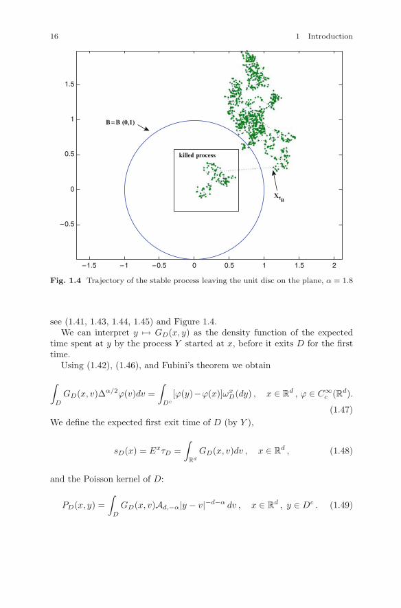
Fig. 1.4 Trajectory of the stable process leaving the unit disc on the plane, α = 1.8
see (1.41, 1.43, 1.44, 1.45) and Figure 1.4.We can interpret y �→ GD(x, y) as the density function of the expected
time spent at y by the process Y started at x, before it exits D for the firsttime.
Using (1.42), (1.46), and Fubini’s theorem we obtain
∫D
GD(x, v)Δα/2ϕ(v)dv =∫
Dc
[ϕ(y)−ϕ(x)]ωxD(dy) , x ∈ R
d , ϕ ∈ C∞c (Rd).
(1.47)We define the expected first exit time of D (by Y ),
sD(x) = ExτD =∫
Rd
GD(x, v)dv , x ∈ Rd , (1.48)
and the Poisson kernel of D:
PD(x, y) =∫
D
GD(x, v)Ad,−α|y − v|−d−α dv , x ∈ Rd , y ∈ Dc . (1.49)
1 Introduction 17
Consider (open) U ⊂ D. By integrating (1.46) against the Lebesgue measurewe obtain
sD(x) = sU (x) +∫
Rd
sD(y)ωxU (dy) , x ∈ R
d , U ⊂ D . (1.50)
Integrating (1.46) against Ad,−α|y − v|−d−α dv on Rd, we get
PD(x, y) = PU (x, y) +∫
PD(z, y)ωxU (dz) , x ∈ U, y ∈ Dc. (1.51)
The reader may attempt interpreting (1.51) as harmonicity of PD(x, y) + δy,see [38]. By considering ϕ approximating 1A for open A ⊂ Dc in (1.47), andby (1.24) and Fubini’s theorem we arrive at the Ikeda-Watanabe formula([95]):
ωxD(A) =
∫A
PD(x, y)dy , x ∈ D . (1.52)
We can interpret (1.49), and (1.52), as follows. Jumping from v ∈ D toy ∈ Dc happens over time with intensity Ad,−α|y − v|−d−α. The intensityis integrated against the occupation time measure, GD(x, v)dv, thus givingPD(x, y).
For a large class of domains (but not for all domains) ωxD(∂D) = 0 for
every x ∈ D, so that
ωxD(dy) = PD(x, y)dy on Dc . (1.53)
In particular, (1.53) holds for domains with the outer cone property (a classof open sets containing finite intersections of bounded Lipschitz domains).This is proved by noting that P x(YτBx
∈ Dc) is bounded away from 0 forx ∈ D and Bx = B(x, 1
2dist(x,Dc)), see the formula (1.57) below. Thus theprocess Y started at x will leave D by a jump (from within Bx) with a positiveprobability. If YτBx
jumps to D \Bx, then this reasoning can be repeated bythe strong Markov property. Since leaving D continuously requires an infinitenumber of such jumps (from balls Bx to D\Bx), the probability of continuousapproach to the boundary is zero, see [27], [152], [154]. Below we will use theobservation for the intersection of a given Lipschitz domain with a ball, seeFigure 2.1.
We note in passing that (1.47) and (1.53) yield the following decompositionof each ϕ ∈ C∞
c (Rd) into a sum of a Green potential and Poisson integral,
ϕ(x) =∫
D
GD(x, v)[−Δα/2ϕ(v)
]dv +
∫Dc
PD(x, y)ϕ(y)dy , x ∈ D ,
(1.54)
where we assumed that D is bounded, hence ωxD(Rd) = 1. One can interpret
the two integrals as resulting from “sources” within D, and jumps between

18 1 Introduction
D and Dc (“tunneling” from sources outside of D). For general domains Dthe picture is somewhat complicated by an additional term related to thecontinuous approach of Yt to ∂D at t = τD, see [38] and [125] for details.
The Green function of the ball is known explicitly:
GBr(x, v) = Bd,α |x− v|α−d
∫ w
0
sα/2−1
(s + 1)d/2ds , x, v ∈ Br , (1.55)
wherew = (r2 − |x|2)(r2 − |v|2)/|x− v|2
and Bd,α = Γ(d/2)/(2απd/2[Γ(α/2)]2), see [25], [133].Also ([78], [33], [43]),
sBr(x) =
Cdα
Ad,−α(r2 − |x|2)α/2 , |x| � r , (1.56)
and
PBr(x, y) = Cd
α
(r2 − |x|2|y|2 − r2
)α/2 1|x− y|d , |x| < r , |y| > r , (1.57)
where Cdα = π1+d/2Γ(d/2) sin(πα/2), see Figures 1.5 and 1.6.
−1 −0.8 −0.6 −0.4 −0.2 0 0.2 0.4 0.6 0.8 10
0.2
0.4
0.6
0.8
1
1.2
1.4
1.6
1.8
2
y
G(x
,y)
α = 0.9
d=1
x=0.8
Fig. 1.5 Green function of (−1, 1)

1 Introduction 19
−3 −2 −1 0 1 2 30
0.5
1
1.5
2
2.5
3
x = 0.8
y
α = 1.3
d =1
P(x
,y)
Fig. 1.6 Poisson kernel of (−1, 1)
The formulas (1.55) and (1.57) are essentially due to Marcel Riesz and dateback to 1938 ([133]). They were completed and interpreted in the presentframework by R. Blumenthal, R. Getoor and D. Ray in 1961 ([25]). Theproof of (1.55) and (1.57) consists of verification of (1.44) for ωx
Br(dy) =
1Bcr(y)Pr(x, y)dy. This is a rather involved procedure, aided by the use of
the inversion, Tx = |x|−2x, where x ∈ Rd \ {0}. We refer to [25], [117] and
[133] for details of the calculation. The explanation of the role of the inversion(and the corresponding Kelvin transform) in obtaining the Poisson kernel ofthe ball, along with the interpretation of the inversion in terms of the processY are given in [41]. For instance ([41]),
GTD(x, y) = |x|α−d|y|α−dGD(Tx, Ty) . (1.58)
Here TD = {Tx : x ∈ D}. We encourage the reader to verify (1.58) forD = R
d.Results similar to (1.55) and (1.57) exist for the complement of the ball
and for half-spaces. In fact they can be obtained from (1.55) and (1.57) byusing (1.58). For half-spaces a different proof of (1.55) and (1.57) (i.e. one notusing the Kelvin transform) was obtained recently as a consequence of thecorresponding results for the relativistic process in [44]. The formula (1.56)was first given in [78], see also [33]. For clarity, we need to emphasize that the

20 1 Introduction
distribution of YτB(x,r), given by (1.57), is concentrated on {y : |y − x| > r},hence with probability one the first exit of Y from B(x, r) is by a jump.
Apart from inversion, scaling is extremely helpful in the potential the-ory of the stable Levy process. Let r > 0. Recall that ν(rA) = r−αν(A),Δα/2ϕr(x) = r−αΔα/2ϕ(x/r), Kα(rx) = rα−dKα(x). By the definition anduniqueness of the Green function and the harmonic measure we see that
ωrxrD(rA) = ωx
D(A) , (1.59)
andGrD(rx, rv) = rα−dGD(x, v) , (1.60)
hencesrD(rx) = rαsD(x) , (1.61)
andPrD(rx, ry) = r−dPD(x, y) . (1.62)
Translation invariance and rotation invariance are equally important buteasier to observe. For example GD+y(x+ y, v + y) = GD(x, v). Together withscaling and inversion the properties help reduce many of our considerationsto the setting of the unit ball centered at the origin.
A function u defined (and Borel measurable) on Rd is called α-harmonic
in an (open) set D if it is harmonic on D for the isotropic α-stable Levyprocess Y : for every open bounded set U such that U ⊆ D we have
u(x) = Exu(YτU) , x ∈ U . (1.63)
We assume here absolute convergence of the integral.A counterpart of Weyl’s lemma holds ([32]) for α-harmonic functions: u is
α-harmonic in D if and only if u is C2 on D, and
Δα/2u(x) = 0 , x ∈ D . (1.64)
We note that for this condition to hold, u must be defined on the whole of Rd,
and its values on Dc are crucial for this property. This reflects the fact thatΔα/2 is a non-local operator allowing for a direct influence between distantpoints x and y in the domain of u, see (1.24). In particular, the followingintegrability assumption holds for α-harmonic function u:
∫Rd
|u(y)|(1 + |y|)d+α
dy < ∞ .
We may also define Δα/2 in a weak (distributional) sense. This allows to con-sider Δα/2 and (Schrodinger operators) Δα/2φ+ qφ as defined locally, i.e. on
1 Introduction 21
arbitrary open sets (in the sense of the L. Schwartz’ theory of distributions),even for discontinuous q which do not have well-defined pointwise values (seebelow). In this connection we like to mention the following observation: if u isα-harmonic on open U1 and u is α-harmonic on open U2 then u is α-harmonicon U1 ∪ U2. This fact is trivial according to (1.64). It can also be proved byusing the probabilistic definition of α-harmonicity (1.63), but such proof is nolonger trivial ([33]). This points out a local aspect of the otherwise non-localproperty of α-harmonicity (the reader interested in more details may consult[32] and [33]). In the remainder of this survey we will not employ the weakfractional Laplacian (we refer the interested reader to [32] for details of thisapproach to Schrodinger operators). We will use a probabilistic methodologybased on the so-called multiplicative functionals and Green functions, ratherthan on infinitesimal generators; and we refer the interested reader to [33] formore.
If u is α-harmonic in a domain containing B(0, r) then
u(x) = Cdα
∫|y|>r
[r2 − |x|2|y|2 − r2
]α/2
|y − x|−du(y)dy , x ∈ B(0, r) . (1.65)
We see that such u is C∞ on B(0, r). For nonnegative u we also obtainHarnack inequality. The next two propositions are versions of it.
Proposition 1.2. If u � 0 on Rd and u is α-harmonic on D ⊃ Bρ ⊃ Br
x1, x2, then
u(x1) �(
1 + r/ρ
1− r/ρ
)d
u(x2) . (1.66)
Proof. If r � s < ρ then by (1.57) we have PBs(x1, z) � (1 + r/s)d(1 −
r/s)−dPBs(x2, z) for |z| � s. Using (1.65) (for B(0, s))), and letting s → ρ,
we prove the result. ��
Proposition 1.3. If x1, x2 ∈ D then there is cx1,x2 such that for every λ � 0
u(x1) � cx1,x2u(x2) . (1.67)
Proof. If x1, x2 ∈ Br ⊂ B2r ⊂ D for some r > 0 then we are done byLemma 1.2 with c = cx1,x2 depending only on d. Assume that B(x1, 2r) ⊂ D,B(x2, 2r) ⊂ D, B(x1, 2r)∩B(x2, 2r) = ∅ for some r > 0, and consider (1.63)with U = B(x1, r). Let y ∈ Dc. By (1.65) and the first part of the proof weobtain u(x1) � c
∫B(x2,r)
u(x2)PBr(0, x− x1)dx = cu(x2). ��
If K ⊂ D is compact and x1, x2 ∈ K then cx1,x2 in Harnack’s inequalityabove may be so chosen to depend only on K, D, and α, because r in theabove proof may be chosen independently of x1, x2. Note that D and K maybe disconnected. This shows a certain advantage of the fact that Y has jumps.

22 1 Introduction
1.1.4 Subordinate Brownian Motions
The rotationally invariant α–stable processes are obtained from the Brownianmotion by a subordination procedure.
Let X = (X(u) : u ≥ 0) be a d-dimensional Brownian motion. Subor-dination of Brownian motion consists of time-changing the paths of X byan independent subordinator. To be more precise, let S = (St : t ≥ 0) bea subordinator (i.e., a nonnegative, increasing Levy process) independent ofX. The process Y = (Yt : t ≥ 0) defined by Yt = X(St) is called a sub-ordinate Brownian motion. The process Y is an example of a rotationallyinvariant d-dimensional Levy process. A general Levy process in R
d is com-pletely characterized by its characteristic triple (b, A, π), where b ∈ R
d, A isa nonnegative definite d×d matrix, and π is a measure on R
d \{0} satisfying∫(1∧|x|2)π(dx) <∞, called the Levy measure of the process. Its characteris-
tic exponent Φ, defined by E[exp{i〈x, Yt〉}] = exp{−tΦ(x)}, x ∈ Rd, is given
by the Levy-Khintchine formula involving the characteristic triple (b, A, π).The main difficulty in studying general Levy processes stems from the factthat the Levy measure π can be quite complicated.
The situation simplifies immensely in the case of subordinate Brownianmotions. If we take the Brownian motion X as given, then Y is completelydetermined by the subordinator S. Hence, one can deduce properties of Yfrom properties of the subordinator S. On the analytic level this translatesto the following: Let φ denote the Laplace exponent of the subordinator S.That is, E[exp{−λSt}] = exp{−tφ(λ)}, λ > 0. Then the characteristic ex-ponent Φ of the subordinate Brownian motion Y takes on the very simpleform Φ(x) = φ(|x|2) (our Brownian motion X runs at twice the usual speed).Hence, properties of Y should follow from properties of the Laplace exponentφ. This will be one of main themes of these lecture notes – we will studypotential-theoretic properties of Y by using information given by φ. Resultsobtained by this approach include explicit formulas for the Green function ofY and the Levy measure of Y . Let p(t, x, y), x, y ∈ R
d, t > 0, denote the tran-sition densities of the Brownian motion X, and let μ, respectively U , denotethe Levy measure, respectively the potential measure, of the subordinator S.Then the Levy measure π of Y is given by π(dx) = J(x) dx, where
J(x) =∫ ∞
0
p(t, 0, x)μ(dt) ,
while the Green function G(x, y), x, y ∈ Rd, of Y is given by
G(x, y) =∫ ∞
0
p(t, x, y)U(dt) .
Let us consider the second formula (same reasoning also applies to the firstone). This formula suggests that the asymptotic behavior of G(x, y) when
1 Introduction 23
|x−y| → 0 (respectively, when |x−y| → ∞) should follow from the asymptoticbehavior of the potential measure U at ∞ (respectively at 0). The latter canbe studied in the case when the potential measure has a monotone densityu with respect to the Lebesgue measure. Indeed, the Laplace transform ofU is given by LU(λ) = 1/φ(λ), hence one can invoke the Tauberian andmonotone density theorems to obtain the asymptotic behavior of U from theasymptotic behavior of φ.
We will be mainly interested in the behavior of the Green function G(x, y)and the jumping function J(x) near zero, hence the reasonable assumptionon φ will be that it is regularly varying at infinity with index α ∈ [0, 1]. Thisincludes subordinators having a drift, as well as subordinators with slowlyvarying Laplace exponent at infinity, for example, a gamma subordinator. Inthe latter case we have φ(λ) = log(1 + λ) and hence α = 0.
1.2 Outline of the Book
Precise boundary estimates and explicit structure of α-harmonic functionson general sub-domains of R
d remained for a long time essentially beyondthe reach of the general theory. They are now objects of the BoundaryPotential Theory which is discussed in Chapters 2 and 3 of the book. Themain results of this theory: the Boundary Harnack Principle, the 3GTheorem, the potential theory of Schrodinger-type perturbations andthe Conditional Gauge Theorem are proven and discussed in Chapter 2.In Chapter 3 we present the important topic of nontangential limits of α-harmonic functions on the border of the domain, whose main result is theRelative Fatou Theorem for α-harmonic functions. Boundary PotentialTheory for relativistic stable processes is also presented in Chapter 3.
The Spectral Theory of stable and related processes is an important toolof the Stochastic Potential Theory. It is the subject of Chapter 4 of the book.Its main results: Intrinsic Ultracontractivity, connection to Steklov problem,eigenvalue estimates, isoperimetric inequalities and estimates of the spectralgap are presented.
The second part of the book, contained in Chapter 5, is devoted to thePotential Theory for Subordinate Brownian motions, processes moregeneral than α–stable processes. Both classical Potential Theory and Bound-ary Potential Theory are presented for the subordinators and the subordinateprocesses. The main examples of subordinate processes covered by these re-sults are stable and relativistic stable processes, geometric stable processesand iterated geometric stable processes. Important classes of gamma subor-dinators and Bessel subordinators are also included. In the last section of thischapter the underlying Brownian motion is replaced by the Brownian motionkilled upon exiting a Lipschitz domain D.
The book has a form of extended lecture notes. We often strive to sug-gest ideas and relationships at the cost of the generality and completeness.

24 1 Introduction
When the ideas are too cumbersome to verbalize, we choose to refer to theoriginal papers. Occasionally, we present new results and modifications orsimplifications of existing proofs. We often employ probabilistic notions andinterpretations because they are extremely valuable for understanding of theideas. They also lead to concise notation and powerful technical tools. Gener-ally speaking, the main perspective that the probabilistic potential theory canoffer is that of the distribution of the underlying process on the path space, asconstructed by Kolmogorov. The distribution is a much richer object than thecorresponding transition probability (or semigroup). The fundamental prop-erty of the distribution is the strong Markov property, first proved by Huntfor the Brownian motion. It should be noted that this property supersedesthe Chapman-Kolmogorov equations allowing for the use of random stoppingtimes–chiefly the first exit times of sub-domains of the state space with thenatural hierarchy given by inclusion of the domains. For instance, the strongMarkov property yields the mean value property for the Green potentials ofmeasures off the support of these measures.

Chapter 2
Boundary Potential Theoryfor Schrodinger Operators Basedon Fractional Laplacian
by K. Bogdan and T. Byczkowski
2.1 Introduction
Precise boundary estimates and explicit structure of harmonic functions areclosely related to the so-called Boundary Harnack Principle (BHP). Theproof of BHP for classical harmonic functions was given in 1977-78 byH. Dahlberg in [65], A. Ancona in [3] and J.-M. Wu in [153] (we also re-fer to [99] for a streamlined exposition and additional results). The resultswere obtained within the realm of the analytic potential theory. A proba-bilistic proof of BHP, one which employs only elementary properties of theBrownian motion, was given in [11]. The proof encouraged subsequent at-tempts to generalize BHP to other processes, in particular to the processesof jump type.
BHP asserts that the ratio u(x)/v(x) of nonnegative functions harmonicon a domain D which vanish outside the domain near a part of the domain’sboundary, ∂D, is bounded inside the domain near this part of ∂D. The resultrequires assumptions on the underlying Markov process and the domain.For Lipschitz domains and harmonic functions of the isotropic α-stable Levyprocess (0 < α < 2), BHP was proved in [27]. Another proof, motivatedby [11], was obtained in [31] and extensions beyond Lipschitz domains wereobtained in [150] and [38]. In particular the results of [38] provide a conclusionof a part of the research in this subject, and offer techniques that may beused for other jump-type processes.
Lipschitz BHP leads to Martin representation of nonnegative α-harmonicfunctions on Lipschitz domains ([28] and [56]). Another important conse-quence of BHP are sharp estimates of the Green function of Lipschitzdomains and the so-called 3G Theorem (see (2.26) below). We give theseapplications in the first part of the chapter, along with a self-contained proofof BHP, following [27] and [38].
In the second part of the chapter we focus on the potential theory ofSchrodinger-type perturbations, Δα/2 +q, of the fractional Laplacian on sub-domains of R
d. The main result we discuss here is the Conditional GaugeTheorem (CGT), asserting comparability of the Green function of Δα/2 + q
K. Bogdan et al., Potential Analysis of Stable Processes and its Extensions,Lecture Notes in Mathematics 1980, DOI 10.1007/978-3-642-02141-1 2,c© Springer-Verlag Berlin Heidelberg 2009
25

26 K. Bogdan and T. Byczkowski
with that of Δα/2, under an assumption of “non-explosion”. Here 0 < α < 2,and the proof of CGT relies on the 3G Theorem, thus on (Lipschitz) BHP.In presenting these results we generally follow the approach of papers [32] and[33]. The approach was modeled after [62], which deals with the Laplacianand its underlying process of the Brownian motion (see [64] for Schrodingerperturbations of elliptic partial differential operators of second order). For adifferent technique we refer to [54]. It should be noted that there are manyalgebraic similarities between the fractional Laplacian (α < 2) and the Lapla-cian (α = 2), but there are also deep analytical differences between these twocases, primarily due to the discontinuity of paths of the isotropic α-stableLevy process for 0 < α < 2.
2.2 Boundary Harnack Principle
Below we freely mix ideas from [27], [31], [32], [150], and [38], with somedidactic improvements and modifications aimed at the simplification of pre-sentation. In particular we give perhaps the shortest existing proof of BHPfor α-harmonic functions.
In what follows nonempty D ⊂ Rd is open. We intend to present the main
ideas of the proof of BHP as given in [38] for arbitrary domains. However,for the simplicity of the discussion in the remainder of this chapter unlessstated otherwise, we will assume that D is a Lipschitz domain, and we willconcentrate on finite nonnegative functions f on R
d, which are representedon D as Poisson integrals of their values on Dc:
f(x) =∫
Dc
f(y)PD(x, y)dy , x ∈ Dc . (2.1)
For instance, if (D is a Lipschitz domain and) f � 0 is bounded on D,then f = PD[f ] on D, see [27]. For a general discussion of the notion of α-harmonicity we refer the reader to [32, 38]. We should perhaps state a warningthat some aspects of the notion are richer and even counter-intuitive whenconfronted with the properties of harmonic functions of local operators. Inparticular, non-negativeness of functions which are α-harmonic on D is usefulonly if assumed on the whole of R
d (rather than merely on D). For instance,if |y| > r, then the function
Br x �→[
supv∈Br
PBr(v, y)
]− PBr
(x, y),
takes on the minimum of zero in a interior point of Br, in stark contrastwith the Harnack inequality. The reader may also want to consider (non-Lipschitz) domains with boundary of positive Lebesgue measure and domains

2 Boundary Potential Theory for Schrodinger Operators 27
Fig. 2.1 D, Br, andouter cone D
Br
with complement of zero Lebesgue measure but positive Riesz capacity, to ap-prehend the complexity of the boundary problems for α-harmonic functions.
For function f � 0 satisfying (2.1) we have Δα/2f(x) = 0 on D, see [32].Furthermore, for every open U ⊂ D we have
f(x) =∫
Uc
f(y)ωxU (dy) , x ∈ U . (2.2)
This follows from (1.51). We emphasize that for the above mean value prop-erty of Poisson integrals it is not necessary that U be a compact subset of D,and we to refer the reader to [38] for cautions needed to deal with the generalnonnegative α-harmonic functions.
When 0 < r � 1 we let Dr = D ∩ Br, a domain with the outer coneproperty, see Figure 2.1. We will often use (2.2) for U = Dr. We note thatωx
Dr(∂Dr) = 0 for x ∈ Dr, in particular we can employ (1.53) for such U .
Consider B = B1 and assume that
f = 0 on B \D . (2.3)
Since GDr� GBr
(see (1.45), (1.46)), by the definition of Poisson kernel(1.49) we get
PDr(x, y) � PBr
(x, y) , x ∈ Dr , y ∈ Bcr .
By the mean value property and the assumption (2.3) we obtain
f(x) �∫
Bcr
f(y)PBr(x, y)dy , x ∈ Br , 0 < r � 1 . (2.4)

28 K. Bogdan and T. Byczkowski
The function PBr(x, y) has a singularity at |y| = r. To remove this inconve-
nience, we will consider an analogue of volume averaging used on occasions inthe classical potential theory. We fix a nonnegative function φ ∈ C∞
c ((1/2, 1))such that
∫ 1
1/2φ(r) dr = 1 and we define
ψ(x, y) =∫ 1
1/2
φ(r)PBr(x, y) dr
= Cdα |y − x|−d
∫ |y|∧1
|y|∧1/2
(r2 − |x|2)α/2
(|y|2 − r2)α/2φ(r)dr , x, y ∈ R
d .
It is not difficult to check that
|ψ(x, y)| � C
(1 + |y|)d+α, |x| � 1/3 , y ∈ R
d . (2.5)
By Fubini’s theorem and (2.4) we obtain
f(x) �∫
Bcr
f(y)ψ(x, y)dy � C
∫Rd
f(y)(1 + |y|)−d−α , x ∈ B1/3 . (2.6)
To obtain a reverse inequality for x ∈ D1 = D ∩ B being not too closeto ∂D1 we note that PBr
(0, y) � Cdαrα|y|−d−α, see (1.57). If r0 > 0 and
B(2r0, x0) ∈ D1, then
f(x0)=∫
Bc(x0,r0)
Pr0(0, y − x0)f(y)dy�∫
Bc(x0,r0)
Cdαrα
0 |y − x0|−d−αf(y)dy.
(2.7)
By the Harnack inequality for f on B(x0, r0) we can enlarge the domain ofintegration so that
f(x0) � c
∫Rd
(1 + |y|)−d−αf(y)dy .
Here and in what follows the constants (c, C etc.) depend on d, α and D, inparticular on r0.
This and (2.6) yield the following Carleson-type estimate.
Corollary 2.1. There is a constant C depending only on d, α, and x0 suchthat
f(x) � Cf(x0) , x, x0 ∈ D1/3 . (2.8)
In what follows we will consider D1/4 and will fix x0 ∈ D1/5. We have
f(x) =∫
Dc1/4
f(y)PD1/4(x, y)dy =∫
D1/4
GD1/4(x, v)κ(v)dv , (2.9)
2 Boundary Potential Theory for Schrodinger Operators 29
whereκ(v) =
∫Dc
1/4
Ad,−α|y − v|−d−αf(y)dy , v ∈ D1/4 .
We thus have f expressed as the Green potential of the charge κ(v) inter-preted as the intensity of jumps of Y “to” f on Dc. Let
κ1(v) =∫
Bc1/3
Ad,−α|y − v|−d−αf(y)dy , v ∈ D1/4 ,
κ2(v) =∫
B1/3\D1/4
Ad,−α|y − v|−d−αf(y)dy , v ∈ D1/4 ,
andfi(x) =
∫D1/4
GD1/4(x, v)κi(v)dv , i = 1, 2 . (2.10)
We note that fi are α-harmonic, in fact Poisson integrals, on D1/4. We observethat κ1 is bounded, in fact nearly constant on D1/4:
c−1κ1(v2) � κ1(v1) � cκ1(v2) , v1, v2 ∈ D1/4 , (2.11)
because |y − v|−d−α is nearly constant in v ∈ D1/4 (uniformly in y ∈ Bc1/3).
Also, κ1(v) � cf(x0), see (2.7). Thus
f1(x) � cf(x0)∫
D1/4
GD1/4(x, v)dv = cf(x0)sD1/4(x) , x ∈ D1/4. (2.12)
We will see that sD1/4 faithfully represents the asymptotics of f = f1 + f2 at∂D ∩B1/5. To this end we first note that by (2.8),
f2(x) � Cf(x0)ωxD1/4
(Bc1/4) , x ∈ D1/4 . (2.13)
Lemma 2.2. For every p ∈ (0, 1) there is a constant C such that if D ⊂ Bthen
ωxD(Bc) � C sD(x) , x ∈ Dp .
Proof. Let 0 < p < 1. We choose a function ϕ ∈ C∞c (Rd) such that 0 � ϕ � 1,
ϕ(y) = 1 if |y| � p, and ϕ(y) = 0 if |y| � 1. Let x ∈ Dp. By (1.47) we have
ωxD(Bc) =
∫Bc
(ϕ(x)− ϕ(y))ωxD(dy) �
∫Dc
(ϕ(x)− ϕ(y))ωxD(dy)
= −∫
D
GD(x, y)Δα/2ϕ(y)dy .
It remains to observe that Δα/2ϕ is bounded and the lemma follows. ��
30 K. Bogdan and T. Byczkowski
By (2.13), scaling and Lemma 2.2 (with p = 4/5) we obtain that f2(x) �cf(x0)sD1/4(x) for x ∈ D1/5. This, and (2.12) yield the following improvementof Carleson estimate
c−1f(x0)sD1/4(x) � f(x) � cf(x0)sD1/4(x) , x ∈ D1/5 . (2.14)
Indeed, the lower bound in (2.14) follows from the inequality
f(x) �∫
D1/4
GD1/4(x, v)κ3(v)dv ,
where
κ3(v) =∫
B(x′,r′)f(y)Ad,−α|y − v|−d−αdy � cf(x0) , v ∈ D1/4 ,
and B(2r′, x′) ⊂ D1/4 \D1/5 is a ball (if the set D1/4 \D1/5 is empty thenf2 ≡ 0, and we simply use (2.11) and (2.10)).
The following Boundary Harnack Principle is a direct analogue of (1.14).
Theorem 2.3 (BHP). If functions f1 and f2 satisfy the above assumptionson f , then
f1(x)f2(y) � Cf1(y)f2(x) , x, y ∈ D1/5 .
Proof. We fix x0 ∈ D ∩B1/5. For x, y ∈ D ∩B1/5 we obtain from (2.14)
f1(x)f2(y) � c2f1(x0)f2(x0)sD1/4(x)sD1/4(y) ,
andf1(y)f2(x) � c−2f1(x0)f2(x0)sD1/4(y)sD1/4(x) .
The result, translation and scaling invariance of the class of α-harmonicfunctions, and the usual Harnack inequality, allow to estimate the growth ofα-harmonic functions vanishing at a part of the domain’s boundary up tothis part of the boundary. The constant C in our present proof depends onD (and the choice of x0), however a more delicate and technical proof showsthat C may be so chosen to depend only on d and α. We refer the reader to[38] for this important strengthening of BHP. An important consequence ofthe domain-independent, or uniform BHP of [38] is given in the followingstatement
limDx→0
f1(x)/f2(x) exists. (2.15)
BHP and (2.15) were given in [27] (see also [31]) for Lipschitz domains,generalized in [150] to the so-called κ-fat domains, and proved for arbitraryopen sets in [38]. The proof of (2.15) seems too technical to be discussed here,but we will hopefully give some insight into its main idea, when discussingthe uniqueness of the Martin kernel with the pole at infinity for cones.
2 Boundary Potential Theory for Schrodinger Operators 31
Let ρ(x) = dist(x,Dc). Compared to BHP, the following local estimatefor individual (nonnegative) Poisson integral on Lipschitz domains, if notsharp, is more explicit.
Lemma 2.4. Let Γ : Rd → R satisfy (1.12), and Γ(0) = 0. Let D = DΓ∩B,
and A = (0, 0, . . . , 0, 1/2) ∈ D. There are C = C(d, α, λ) and ε = ε(d, α, λ) ∈(0, α) such that
C−1f(A)ρ(x)α−ε � f(x) � Cf(A)ρ(x)ε , x ∈ D1/2 . (2.16)
The right hand side of (2.16) is a strengthening of the Carleson estimate,and it asserts a power-type decay of u at the boundary of D. This decay rateis related to the existence of outer cones for the boundary points of D, andsteady escape of mass of the process when it approaches ∂D (see our discus-sion above of the fact that ωx
D(∂D) = 0). For a class of domains includingdomains with the boundary defined by a C2 function we have ε = α/2, whichmay be verified by a direct calculation involving the Green function of theball, and of the complement of the ball, see [56], [109]. Then (2.16) becomessharp, meaning that all sides of the inequality are in fact comparable. Theexponent α/2 is also related to the fact that
f(x) = xα/2+ , x ∈ R , (2.17)
is α-harmonic on the half-line {x > 0}, see [30] for explicit calculations in-volving Δα/2.
For general Lipschitz domains the exponent ε on the right-hand side of(2.16) is usually not given explicitly. We like to note that ε > 0 may be arbi-trarily small, e.g. for the complement of cone with sufficiently small openingin dimension d > 2. For a more detailed study of the asymptotic behavior ofα-harmonic functions in cones, and some open problems we refer the readerto [5] and [123].
We will briefly discuss the left hand side inequality in (2.16). We like toemphasize the fact that the power-type decay cannot be arbitrarily fast, asignificant difference when compared with the classical harmonic functionsin narrow cones. Indeed, ε > 0 may be arbitrarily small (for very narrowcones), but we always have α−ε < α! This is a noteworthy contrast with theclassical potential theory (α = 2). For an explanation of this phenomenon wewill consider exponentially shrinking disjoint balls Bk = B(Ak, crk), where0 < r < 1 and c are such that Bk ⊂ Drk (k = 0, 1, . . .), see Figure 2.2. Bythe mean value property, we have
f(Ak) �k−1∑l=0
∫Bl
f(y)ωAk
Bk(dy) (2.18)
� C
k−1∑l=0
∫Bl
f(Al)r(k−l)α ,

32 K. Bogdan and T. Byczkowski
Fig. 2.2 Exponentiallyshrinking balls
Ak
Bk
Bι
Aι
A0
B0
0
where we used the formula for the Poisson kernel of the ball. Thus, βk :=f(Ak)r−kα � C
∑k−1l=0 βl. By induction we see that βk � C(1+C)kβ0, which
yields the exponent α− ε < α on the left hand side of (2.16).We note that the first term of the sum in (2.18) approximately equals
rkαf(A0), which is much smaller than the whole sum. Thus a direct jump (say,to B0) has a negligible impact on the values of the α-harmonic function onBk. Instead, the many combined shorter jumps between the balls {Bl} yieldthe main contribution. The geometry of Lipschitz domains plays a role here.Domains which are “thinner” at some boundary points may show a differentdecay rate of α-harmonic functions (i.e. that given by a few direct jumpsmay prevail, see [125]). This observation leads to a notion of inaccessibilitydeveloped in [38].
We want to point out after [38], that BHP can be studied as a propertyof the Poisson kernel and the Green function, without even referring to thenotion of α-harmonicity. In fact, the main application of BHP is the followingone, to f1(x) = GD(x, x1) and f2(x) = GD(x, x2), for x (in a Lipschitz subsetof) D \ {x1, x2}. We fix an arbitrary reference point x0 ∈ D and we definethe Martin kernel of D,
MD(x, y) = limDv→y
GD(x, v)GD(x0, v)
, x ∈ Rd , y ∈ ∂D . (2.19)
Theorem 2.5. The limit in (2.19) exists. x �→ MD(x, y) is up to constantmultiples the only nonnegative α-harmonic function on D and equal to zeroon Dc which continuously vanishes at Dc \ {y}.

2 Boundary Potential Theory for Schrodinger Operators 33
The existence part of the result follows easily from (2.15). The α-harmonicity of MD, however, depends delicately on the Lipschitz geometryof the domain via the lower bound in (2.16), see [28]. We refer the readerto [28] for an elementary study of the properties of MD(·, y) for Lipschitzdomains. We also refer to [38] for the case of arbitrary open set and for theexplanation of the role played by the accessibility of the point y from withinthe set.
It should be noted that MD(·, y) is not of the form (2.1). Nonnegativeα-harmonic functions vanishing on Dc are called singular α-harmonic. Theyresemble classical Poisson integrals of singular measures on the sphere (andalso nonnegative martingales converging to zero almost surely).
We will cite after [28] the representation theorem for nonnegative α-harmonic functions on bounded Lipschitz domains D (for arbitrary nonemptyopen subsets of R
d see [38]).
Theorem 2.6. For every function u � 0 which is α-harmonic in D thereexists a unique finite measure μ � 0 on ∂D, such that
u(x) =∫
Dc
PD(x, y)u(y)dy +∫
∂D
MD(x, y)μ(dy) , x ∈ D . (2.20)
In view of the recent developments in [38] we like to make the followingcomments. First,
∫Dc PD(x, y)u(y)dy above may be generalized to Poisson
integrals of nonnegative measures:
∫Dc
PD(x, y)λ(dy) < ∞ , (2.21)
and it is legitimate to regard Dc as the “Martin boundary” of (boundedLipschitz) D for Δα/2, with kernels MD(·, y), y ∈ ∂D, and PD(·, y) + δy(·),y ∈ Dc \ ∂D. Second, for general domains in arbitrary dimension, inaccessi-ble points of the Euclidean boundary will contribute a Poisson kernel, ratherthan a Martin kernel. Third, for unbounded domains a Martin kernel maybe attributed to the point at infinity (if accessible). For details we refer thereader to [38], which appears to finalize the problem of representing nonneg-ative α-harmonic functions, and offers notions and methods appropriate forhandling more general Markov processes with jumps. To further encouragethe interested reader, we want to point out that for bounded domains their“Martin boundary” decreases when the domain increases [38]. Comparing toΔ, we see that the potential theory of Δα/2 is more compatible with theEuclidean topology of R
d.We return to considering a Lipschitz domain D ⊂ R
d in dimension d � 2.For y ∈ ∂D, MD(x, y) is (up to constant multiples) the unique α-harmonicfunction continuously vanishing on Dc \ {y} (and having a singularity at y,

34 K. Bogdan and T. Byczkowski
which “feeds” the function through (1.63)). As remarked above, a similarfunction can be constructed for the point at infinity, if D is unbounded:
M(x) = MD(x,∞) = limDv,|v|→∞
GD(x, v)GD(x0, v)
, x ∈ Rd . (2.22)
In the case when D is an open cone C ⊂ Rd, the existence, uniqueness and
homogeneity properties of M were studied [5] and [123]. Below we will give aflavor of the technique used in the study. We first note that the mean valueproperty holds for such M for every bounded open subset U of C, as thepole is so far away. Let 1 �= 0 be a point in R
d (say 1 = (0, . . . , 0, 1)). Forx ∈ R
d\{0}, we denote by θ(x) the angle between x and 1. The right circularcone of angle Θ ∈ (0, π) is the Lipschitz domain
C = CΘ = {x ∈ Rd : θ(x) < Θ} .
Clearly, for every r > 0 we have rC = C. In particular, by scaling, if u isα-harmonic on C, then so is x �→ u(rx). We will prove the uniqueness of M .To this end, we assume that there is another function m � 0 on R
d whichvanishes on Cc, satisfies m(1) = 1 and
m(x) = Exm(YτB) , x ∈ R
d ,
for every open bounded B ⊂ C. By BHP,
C−1m(x) � M(x) � Cm(x) ,
for x ∈ B ∩ C. By scaling, this extends to all x ∈ C with the same constant.We let a = infx∈C m(x)/M(x). For clarity, we note that C−1 � a � 1. LetR(x) = m(x)− aM(x), so that R � 0 on R
d. Assume (falsely) that R(x) > 0for some, and therefore for every x ∈ C. Then, by BHP and scaling,
R(x) � εM(x) , x ∈ Rd,
for some ε > 0. We have
a = infx∈C
m(x)M(x)
= infx∈C
aM(x) + R(x)M(x)
� a + ε ,
which is a contradiction. Thus R ≡ 0, m = aM , and the normalizing condi-tion m(1) = M(1) = 1 yields a = 1. The uniqueness of M is verified.
We like to note that the existence of the limits of the ratios of nonnegativeα-harmonic functions, (2.15), is proved by a similar argument, see [27, 38].This oscillation-reducing mechanism of BHP is well known for local op-erators, e.g. Laplacian ([11]), but the non-local character of the fractionalLaplacian seriously complicates such arguments, except in some special cases,
2 Boundary Potential Theory for Schrodinger Operators 35
like that of the cone. Some elements of the proof (of vanishing of oscillations ofratios of non-negative α-harmonic functions) are given in [27]. The completedetails in the generality of arbitrary domains are given in [38].
To appreciate the importance of uniqueness, we return to the discussion ofthe Martin kernel with the pole at infinity for the cone. By scaling, for everyk > 0 the function M(kx)/M(k1) satisfies the hypotheses defining M . Thusit is equal to M , or
M(kx) = M(x)M(k1) x ∈ Rd .
In particular, M(kl1) = M(l1)M(k1) for positive k, l. By continuity of α-harmonic functions on the domain of harmonicity, there exists β such thatM(k1) = kβM(1) = kβ and
M(kx) = kβM(x) , x ∈ Rd ,
orM(x) = |x|βM(x/|x|) , x �= 0 , (2.23)
compare (2.16). By (2.14), M is locally bounded and tends to zero at theorigin, thus
0 < β < α . (2.24)
It is known that β is close to α for very narrow cones, and it will be close to0 for obtuse cones (for Θ close to π), at least in dimension d � 2. We referthe reader to [5], [123], [35] for more information and a few explicit values ofβ for specific cones (see (2.17) for the half-line).
2.3 Approximate Factorization of Green Function
In this section we will consider a bounded Lipschitz domain D ⊂ Rd, d � 2,
with Lipschitz constant λ. To simplify formulas, we recall the notation ≈: wewrite f(y) ≈ g(y) for y ∈ A if there exist constants C1, C2 not depending ony such that C1 f(y) � g(y) � C2 f(y), y ∈ A.
Let δ(x) = dist(x,Dc). We fix x0, x1 ∈ D, x0 �= x1, and we let κ =1/(2
√1 + λ2). For x, y ∈ D we denote r = r(x, y) = δ(x)∨δ(y)∨ | x−y |. For
small r > 0 we write B(x, y) for the set of points A such that B(A, κr) ⊂ D∩B(x, 3r)∩B(y, 3r), see Figure 2.3, and we put B(x, y) = {x1} for large r [29].The set B(x, y) is nonempty (see [98] or [29] for details). Informally speaking,A ∈ B(x, y) dominates x and y similarly as A of Lemma 2.4 dominates thepoints of D1/2, see Figure 2.3. Let G = GD, the Green function of D for thefractional Laplacian. We define
φ(x) = G(x0, x) ∧ c .

36 K. Bogdan and T. Byczkowski
Fig. 2.3 A ∈ B(x, y)
x0 x1
A
x y
The following is a sharp, if not completely explicit, approximate factorizationof G(x, y).
C−1 φ(x)φ(y)φ2(A)
|x− y|α−d � G(x, y) � Cφ(x)φ(y)φ2(A)
|x− y|α−d . (2.25)
Here A is an arbitrary point of B(x, y). A proof of (2.25) is given in [98] (seealso [29] for the case of α = 2). We will sketch the proof.
If x and y are close to each other but far from the boundary, then (2.25)is equivalent to G(x, y) ≈ |x − y|α−d, because the term subtracted in (1.45)is small.
Another case to consider is the situation of |y − x| being large and δ(x),δ(y) being small. By symmetry, G(x, y) is α-harmonic both in x, and in y(on D \{y} and D \{x}, correspondingly). By BHP (and the usual Harnackinequality) G(x, y)/G(x0, y) ≈ G(x, x1)/G(x0, x1). Since 0 < G(x0, x1) < ∞is a constant, we obtain (2.25) in the considered case. If |y − x|, δ(x), andδ(y) are all small then we use BHP in a similar way, but twice. If δ(x) issmall, and δ(y) is large, then G(x, y) = G(y, x) ≈ G(x0, x) by the Harnackinequality.
We remark that φ(·) may be replaced by sD(·) in (2.25), compareLemma 2.2, [38]. For bounded C2 domains we may use φ(·) = δα/2(·),obtaining an estimate which is both sharp and explicit, [109, 56].
We will give a short proof of the following celebrated inequality known as3G Theorem:
Theorem 2.7 (3G).
G(x, y)G(y, z)G(x, z)
� C|x− y|α−d|y − z|α−d
|x− z|α−d, x, y, z ∈ D . (2.26)
Proof. let x, y, z ∈ D and R ∈ B(x, y), S ∈ B(y, z), T ∈ B(x, z). By (2.25),
G(x, y)G(y, z)G(x, z)
� C|x− y|α−d|y − z|α−d
|x− z|α−dW 2,

2 Boundary Potential Theory for Schrodinger Operators 37
where W = [φ(y)φ(T )]/[φ(R)φ(S)]. We will verify the boundedness of W . Letr1 = δ(x)∨δ(y)∨|x−y|, r2 = δ(y)∨δ(z)∨|y−z|, and r3 = δ(x)∨δ(z)∨|x−z|because φ is bounded. If R = x1 and S = x1 then W � C. If R �= x1, that is ifr1 is small, then we choose Q ∈ ∂D such that δ(y) = |y−Q|. By the Carlesonestimate φ(y) � Cφ(R). Consequently, if S = x1, then W � C. The sameholds true if S �= x1 and R = x1. By symmetry, to complete the proof, wemay assume that r1 � r2 are small. We have r3 � r1 + r2 � 2r2, so r3 is alsosmall. In fact |T−Q| � |T−z|+|y−z|+|y−Q| < 3r3+r2+r2 � 8r2, thereforeby the Carleson estimate and the Harnack inequality φ(T ) � Cφ(S). Recallthat φ(y) � Cφ(R), thus W is bounded in this case, too. This finishes theproof. ��
Since |x − y|α−d|y − z|α−d/|x − z|α−d � 2d−α(|x− y|α−d + |y − z|α−d
),
we obtain the following version of 3G:
G(x, y)G(y, z)G(x, z)
� C (Kα(x− y) + Kα(y − z)) , x, y ∈ D . (2.27)
The definition of the Martin kernel yields
G(x, y)MD(y, ξ)MD(x, ξ)
� C (Kα(x− y) + Kα(y − ξ)) , x, y ∈ D , ξ ∈ ∂D .
(2.28)
As we have mentioned, the importance of 3G in potential theory was ob-served in [64]. Below we will use a probabilistic framework of conditionalprocesses to employ 3G to construct and estimate the Green function ofSchrodinger perturbations of Δα/2. Before we take our chances in this en-deavor, however, we like to notice that a purely analytic approach to thisproblem also exists. The approach is based on the so called perturbation se-ries, or Duhamel’s formula, whose application is greatly simplified if 3G issatisfied. We refer the reader to a self-contained exposition of this techniquein [85] (see also [84]). Analogous consideration based on so-called 3P The-orem of [36] yields comparability of the perturbed transition density withthe original one. We refer the interested reader to [36] and [37] for thesedevelopments.
2.4 Schrodinger Operator and ConditionalGauge Theorem
We will focus on the potential theory of Schrodinger operators, u �→ Δα/2u+qu, on subdomains of R
d, following the development of [32, 33, 62]. The classof admissible “potentials” q is tailor-made for the transition probability of{Yt} (and Δα/2).

38 K. Bogdan and T. Byczkowski
Put in a general perspective we consider here “small” additive perturba-tions of the generator of a semigroup and we expect the potential-theoreticobject to be similar before and after these perturbations. In particular, theconditional gauge function defined below is the ratio between the Green func-tions after and before the perturbation, and the Conditional Gauge Theorem(CGT) asserts that the function is bounded under certain assumptions. Orig-inally, many authors considered the Laplace operator and bounded q, or q ina Kato class and smooth domains D, see the references in [64]. The paper[64] made an essential progress by including Lipschitz domains in the case ofthe Laplace operator. This direction of research is summarized in [62].
The paper [54] initiated in 1997 the study of CGT for rotation invariantstable Levy and more general processes for Schrodinger and more generalperturbations. The focus of [54] was on C1,1 domains. CGT for the stableproceses in Lipschitz domains was proved in 1999 in [32]. We also like to notethat there is a recent non-probabilistic approach to CGT, see [85] and [37].
A (Borel) function q on Rd is said to belong to the Kato class Jα if
limt↓0
supx∈Rd
∫ t
0
Ex|q(Ys)| ds = 0 . (2.29)
Thus, (2.29) is a statement of negligibility of q in (small) time, with respectto the given transition probability. To make (2.32) more explicit we recall thefollowing well-known estimate (see (1.29)):
C−1
(t
|x|d+α∧ t−d/α
)≤ pt(x) ≤ C
(t
|x|d+α∧ t−d/α
). (2.30)
The estimate is proved by subordination (see, e.g., [39]). Noteworthy,
t
|x|d+α≤ t−d/α iff t ≤ |x|α . (2.31)
We easily see that
∫ t
0
ps(x)ds ≈ t2
|x|d+α∧ 1|x|α−d
.
By the definition of Ex, and Fubini-Tonelli, q ∈ Jα if and only if
limt↓0
supx∈Rd
∫Rd
[t2
|y − x|d+α∧ 1|y − x|α−d
]|q(y)|dy = 0 .
2 Boundary Potential Theory for Schrodinger Operators 39
It follows that (2.29) is equivalent to the following condition of negligibilityof q in (small) space with respect to the potential operator:
limγ↓0
supx∈Rd
∫|x−y|≤γ
Kα(x− y) |q(y)| dy = 0 . (2.32)
We also note that L∞(Rd) ⊂ Jα ⊂ L1loc(R
d).For q ∈ Jα we define the additive functional
Aq(t) =∫ t
0
q(Ys) ds ,
and the corresponding multiplicative functional
eq(t) = exp(Aq(t)) .
We haveeq(t + s) = eq(t) (eq(s) ◦ θt) , t, s � 0 .
Here θt is the usual shift operator acting on the process Y by the formula:Ys ◦ θt = Yt+s.
For an open bounded set D we define the killed Feynman-Kac semigroupTt by the formula
Tt f(x) = Ex[t < τD; eq(t) f(Yt)] . (2.33)
Tt is a strongly continuous semigroup on Lp(D), 1 � p <∞, and on C(D)–for regular D. For each t > 0, the operator Tt is determined by a symmetrictransition density function ut(x, y) which is in C0(D×D) for regular D. Weshould note that {Tt , t > 0} is generated by Δα/2 + q, see [32]. The nextlemma is fundamental in the theory of Feynman-Kac semigroups– this is seenin the development of [62], which we will follow quite closely below.
Lemma 2.8. [Khasminski lemma] Let τ be an optional time of Y such that
τ � t + τ ◦ θt , on {t < τ} , t > 0 . (2.34)
Suppose that q � 0 and ExA(τ) < ∞ for all x ∈ Rd. Then for each integer
n � 0 we have,sup
xEx[A(τ)n] � n! sup
x(ExA(τ))n . (2.35)
If supx ExA(τ) = α < 1 then
supx
ExeA(τ) � (1− α)−1 .

40 K. Bogdan and T. Byczkowski
The condition (2.34) is satisfied if τ is constant or if τ = τD for someD ⊆ R
d.
Proof. Since q � 0, the functional A(·) is nonnegative and nondecreasing. ByFubini-Tonelli and (2.29), A(τ) < ∞ a.s. We have
A(τ)n+1
n + 1=∫ τ
0
[A(τ)−A(t)]n dA(t) .
For t < τ , by (2.34),
A(τ)−A(t) � A(t + τ ◦ θt)−A(t) =∫ t+τ◦θt
t
q(Ys) ds
= [∫ τ
0
q(Ys) ds] ◦ θt = A(τ) ◦ θt .
By Fubini’s theorem,
Ex[A(τ)n+1]n + 1
� Ex[∫ τ
0
[A(τ) ◦ θt]n dA(t)] =∫ ∞
0
Ex[t < τ ; [A(τ) ◦ θt]nq(Yt)] dt .
By the Markov property the last integral is equal to
∫ ∞
0
Ex[t < τ ;EYt [A(τ)n] q(Yt)] dt � supx
Ex[A(τ)n]∫ ∞
0
Ex[t < τ ; q(Yt)] dt
= supx
Ex[A(τ)n]ExA(τ) .
It follows that
supx
Ex[A(τ)n+1] � (n + 1) supx
Ex[A(τ)n] supx
Ex[A(τ)] ,
hence (2.35) is proved by induction on n. The last assertion of the lemma isan immediate consequence of (2.35). ��
We like to note that A(t) increases where q > 0, and eq(t) may be inter-preted as the mass of a particle moving along the trajectories of the processin the potential well given by q. If q � 0 then the mass is always bounded by1 (subprobabilistic), which corresponds to Courrege’s theorem, see (1.25).
The gauge function of D and q is defined as follows:
u(x) = Exeq(τD) .
We can interpret u(x) as the expected mass of the particle when it leavesthe domain. We note that since τD is an unbounded random variable, themass may be infinite if q is (say, positive and) large enough. When the gauge
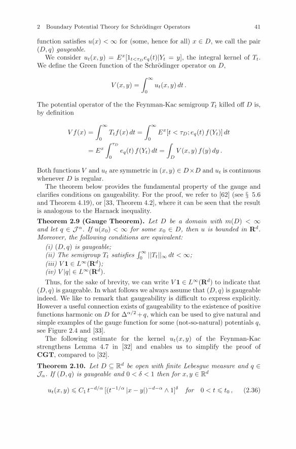
2 Boundary Potential Theory for Schrodinger Operators 41
function satisfies u(x) < ∞ for (some, hence for all) x ∈ D, we call the pair(D, q) gaugeable.
We consider ut(x, y) = Ex[1t<τDeq(t)|Yt = y], the integral kernel of Tt.
We define the Green function of the Schrodinger operator on D,
V (x, y) =∫ ∞
0
ut(x, y) dt .
The potential operator of the the Feynman-Kac semigroup Tt killed off D is,by definition
V f(x) =∫ ∞
0
Ttf(x) dt =∫ ∞
0
Ex[t < τD; eq(t) f(Yt)] dt
= Ex
∫ τD
0
eq(t) f(Yt) dt =∫
D
V (x, y) f(y) dy .
Both functions V and ut are symmetric in (x, y) ∈ D×D and ut is continuouswhenever D is regular.
The theorem below provides the fundamental property of the gauge andclarifies conditions on gaugeability. For the proof, we refer to [62] (see § 5.6and Theorem 4.19), or [33, Theorem 4.2], where it can be seen that the resultis analogous to the Harnack inequality.
Theorem 2.9 (Gauge Theorem). Let D be a domain with m(D) < ∞and let q ∈ J α. If u(x0) < ∞ for some x0 ∈ D, then u is bounded in Rd.Moreover, the following conditions are equivalent:
(i) (D, q) is gaugeable;(ii) The semigroup Tt satisfies
∫∞0||Tt||∞ dt < ∞;
(iii) V 1 ∈ L∞(Rd);(iv) V |q| ∈ L∞(Rd).
Thus, for the sake of brevity, we can write V 1 ∈ L∞(Rd) to indicate that(D, q) is gaugeable. In what follows we always assume that (D, q) is gaugeableindeed. We like to remark that gaugeability is difficult to express explicitly.However a useful connection exists of gaugeability to the existence of positivefunctions harmonic on D for Δα/2 +q, which can be used to give natural andsimple examples of the gauge function for some (not-so-natural) potentials q,see Figure 2.4 and [33].
The following estimate for the kernel ut(x, y) of the Feynman-Kacstrengthens Lemma 4.7 in [32] and enables us to simplify the proof ofCGT, compared to [32].
Theorem 2.10. Let D ⊆ Rd be open with finite Lebesgue measure and q ∈
Jα. If (D, q) is gaugeable and 0 < δ < 1 then for x, y ∈ Rd
ut(x, y) � C1 t−d/α [(t−1/α |x− y|)−d−α ∧ 1]δ for 0 < t � t0 , (2.36)
42 K. Bogdan and T. Byczkowski
−2 −1.5 −1 −0.5 0 0.5 1 1.5 20
0.5
1
1.5
2
2.5
3
α = 0.7
d = 1
x
u D(x
)
Fig. 2.4 A gauge function for q � 0, see [33]
where t0 = t0(δ, q, α), C1 = C1(d, α) and
ut(x, y) � C2 exp (−β t), for t > t0 , (2.37)
where C2 = C2(D, d, α), β = β(δ, q, α) . Furthermore, if D is additionallybounded then
V (x, y) � C3 |x− y|α−d . (2.38)
Proof. Let p > 1 be fixed. Choose t0 > 0 such that for 0 < t � t0
supx∈D
Ex[e2pq(t)] � 2 .
For 0 < t � t0 and f ∈ L2(D) define Stf(x) = Ex[t < τD; epq(t) f(Yt)]. BySchwarz inequality, for 0 < t < t0 we have
|Stf(x)|2 � Ex[t < τD; e2pq(t)]Ex[t < τD; f(Yt)2] � 2Ex[f(Yt)2]
= 2∫
f(y)2 pt(x, y) dy � 2 t−d/α ||f ||22 supx
p1(x) .
Thus, we have obtained
||St||2,∞ � C t−d/2α .

2 Boundary Potential Theory for Schrodinger Operators 43
Now, observe that for positive f ∈ L1 and positive φ ∈ L2 we have∫
φ Stf dx =∫
f Stφ dx � ||Stφ||∞∫
f dm � ||St||2,∞ ||φ||2 ||f ||1 .
This shows that Stf ∈ L2 and ||St||1,2 � ||St||2,∞. If f ∈ L1 we have Stf =St/2St/2f ∈ L∞ so
||St||1,∞ � ||St/2||1,2 ||St/2||2,∞ � ||St/2||22,∞ � C t−d/α .
Let B be a Borel subset of D. Then
Tt1B(x) � Ex[t < τD; epq(t)1B(Yt)]1−δ Ex[t < τD; 1B(Yt)]δ
= (St1B(x))1−δ (PD
t 1B(x))δ
� ||St||1−δ1,∞ m(B)1−δ [C1 t−d/α ((t−1/α ρ)−d−α ∧ 1)m(B)]δ
� C t−(1−δ)d/α m(B) [C1 t−d/α ((t−1/α ρ)−d−α ∧ 1)]δ
� C3 t−d/α m(B) [(t−1/α ρ)−d−α ∧ 1]δ ,
where ρ = supy∈B |x− y| and we applied the fact that
pDt (x, y) � pt(x, y) = t−d/α p1(t−1/α(x− y))
� C1 t−d/α [(t−1/α|x− y|)−d−α ∧ 1] , t > 0 , x, y ∈ Rd .
Thus, we have obtained
1m(B)
∫B
ut(x, y) dy � C3 t−d/α m(B) [(t−1/α ρ)−d−α ∧ 1]δ .
Consider B = B(y0, δ) and x, y0 ∈ D. Letting δ ↓ 0, we obtain
ut(x, y) � C3 t−d/α [(t−1/α |x− y|)−d−α ∧ 1]δ ,
which gives (2.36). Since (D, q) is gaugeable, by Theorem 2.5 we obtain
||Tt||1 � C e−εt ,
for t > t0 and for some ε > 0. On the other hand
1m(B)
∫ut(x, y)1B(y) dy = ||Tt||1,∞ .
As before, this gives ut(x, y) � ||Tt||1,∞ . Since
||Tt||1,∞ � ||Tt0 ||1,∞ ||Tt−t0 ||1 � ||Tt0 ||1,∞ C e−ε(t−t0) ,

44 K. Bogdan and T. Byczkowski
we obtain (2.37). To prove (2.38) we apply (2.36) to estimate
C−11
∫ t0
0
ut(x, y) dt �∫ t0
0
t−d/α[1 ∧ (t−1/α|x− y|)−d−α]δ dt
=∫ t0
0
t−d/α[1 ∧(
t
|x− y|α)−d−α
]δ dt
= |x− y|−δ(d+α)
∫ |x−y|α∧t0
0
tδ−(1−δ)d/α dt
+∫ t0
|x−y|α∧t0
t−d/α dt .
In the first integral on the right hand-side we take a δ > 0 such that d/α <1+δ1−δ , and we then see that the first integral is convergent. We obtain theupper bound
C4|x− y|−δ(d+α)|x− y|(1−d/α+δ(1+d/α))α
+ C5|x− y|α−d = C |x− y|α−d .
To finish the proof we observe that (2.37) yields∫ ∞
t0
ut(x, y) dt � β−1e−βt0 ,
which, together with the observation that |x− y| � diam(D), concludes theproof of (2.38). ��
We note that since ut(x, y) is continuous, the above estimate yields thecontinuity of V (x, y) for x, y ∈ R
d, x �= y, under the assumption that D isregular (and bounded).
We should also mention that there exists a new method of estimating ut
based on the notion of conditional smallness of q which yields comparabilityof ut and pt in finite time, see [36].
The following lemma is a well-known but fundamental relationship be-tween GD and V , see [62], Ch. 6. For an analyst, the lemma is an instance ofthe (implicit) perturbation formula for V , compare [85].
Lemma 2.11. Suppose that q ∈ Jα and V 1 ∈ L∞(D). If V |q|GD |f | < ∞on D then
V f = GD f + V q GD f .
Proof. By Fubini’s theorem we obtain
V q GD f(x) = Ex
∫ τD
0
eq(t) q(Yt)EYt [∫ τD
0
f(Ys) ds] dt
= Ex
∫ τD
0
eq(t) q(Yt)∫ τD
t
f(Ys) ds dt

2 Boundary Potential Theory for Schrodinger Operators 45
= Ex
∫ τD
0
f(Ys)∫ τD
s
eq(t) q(Yt) dt ds
= Ex
∫ τD
0
f(Ys) [eq(s)− 1] ds = V f(x)−GDf(x) .
The application of Fubini’s theorem is justified by the condition V |q|GD |f |< ∞. ��
An important consequence of the above lemma and Theorem 2.10 is thefollowing
Lemma 2.12. Suppose that q ∈ Jα and V 1 ∈ L∞(D). Assume that D isbounded and regular. Then for every x, y ∈ D, x �= y we have
V (x, y) = GD(x, y) +∫
D
V (x,w) q(w)GD(w, y) dw . (2.39)
Proof. Applying the preceding lemma we obtain that for every x ∈ D theequation (2.39) holds y-almost everywhere. Assume that |x − y| > δ > 0.Then either |x− w| > δ/2 or |w − y| > δ/2. Suppose that the first conditionholds. Then, by Theorem 2.10 we obtain
V (x,w) � C Kα(x,w) � C Kα(δ/2) so
V (x,w) |q(w)|GD(w, y) � C Kα(δ/2) |q(w)|Kα(w − y) .
In the second case we obtain
V (x,w) |q(w)|GD(w, y) � C Kα(x− w) |q(w)|Kα(δ/2) .
Consequently, when |x− y| > δ we have
V (x,w) |q(w)|GD(w, y) � C Kα(δ/2) |q(w)| [Kα(w − y) + Kα(x− w)] .
Since D is bounded, it follows that the set of functions
{w �→ V (x,w) q(w)GD(w, y); (x, y) ∈ D ×D, |x− y| > δ}
is uniformly integrable on D. On the other hand, for each w ∈ D, the function
(x, y) �→ V (x,w) q(w)GD(w, y)
is continuous except possibly at x = w or y = w. Therefore, the integral onthe right-hand side of (2.39) is continuous in (x, y) ∈ D × D, |x − y| > δ.Since δ is arbitrary, both members of (2.39) are continuous in (x, y) ∈ D×D,x �= y. The proof is complete. ��

46 K. Bogdan and T. Byczkowski
Let h be an α-harmonic and positive on a bounded domain D. By pDt (x, y)
we denote the transition density function of (Yt) killed on exiting D. Forx, y ∈ D and t > 0 we define time-homogeneous transition density (of Doob’sh-process)
ph(t;x, y) = h(x)−1 pDt (x, y)h(y) .
This defines a strong Markov process on D∂ = D∪{∂}. Here ∂ is the absorb-ing state (cemetery) attached to the state space to accommodate for the lossof mass (the conditional process is generally subprobabilistic if consideredon the original state space, [23]). The h-process is denoted also by Yt, whilethe corresponding expectations and probabilities are denoted by Ex
h , P xh . We
should note that even though we use the same generic notation for the condi-tional process, there is no pathwise correspondence between the original andthe conditional processes, and theorems involving the conditional process areusually more difficult.
The definition of the h-process yields,
Exh [t < τD; f(Yt)] = h(x)−1 Ex[t < τD; f(Yt)h(Yt)] . (2.40)
Let D be a bounded Lipschitz domain; for fixed ξ ∈ ∂D we put
h(y) = MD(y, ξ) .
Here MD(·, ξ) is Martin’s kernel of D, which is α-harmonic in D [27, 38].We also need another version of conditioning: for fixed y ∈ D we let
h(y) = GD(y, z) .
The function h above is α-harmonic in D \ {z}, and superharmonic in D, see[56]. In the sequel, we will use the notation Ex
ξ , P xξ (Ex
z , P xz , respectively) to
indicate conditioning by Martin kernel (Green function, respectively).We redefine α-stable ξ-Levy motion Yt by putting Ys = ξ for s � τD to get
the process on D∪{ξ}. Analogously, α-stable z-Levy motion Yt is defined onD and Ys = z for s � τD\{z}.
For a stopping time T � τD\{y} we obtain a specialization of the formula(2.40):
Exz [T < τD\{y}; f(YT )] = GD(x, z)−1 Ex[T < τD; f(YT )GD(YT , z))] . (2.41)
A similar formula holds true for the ξ-process.
As an instructive exercise we compute the Green function of α-stablez-Levy motion.
Proposition 2.13 (Green function for conditional process). Let Dbe a bounded Lipschitz domain in R
d, α < d, Yt - α-stable z-Levy motion.The Green function of D, as the function of y, computed for the process Y
2 Boundary Potential Theory for Schrodinger Operators 47
(starting at x ∈ D and exiting at z ∈ D) has the following form:
GD(x, y)GD(y, z)GD(x, y)
.
Proof. Indeed, we obtain
Exz
∫ τD\{z}
0
f(Yt) dt =∫ ∞
0
Exz [t < τD\{z}; f(Yt)] dt
=∫ ∞
0
GD(x, z)−1Ex[t < τD\{z}; f(Yt)GD(Yt, z)] dt
= GD(x, z)−1Ex
∫ τD
0
f(Yt)GD(Yt, z) dt
= GD(x, z)−1GD(f(·)GD(·, z))(x)
=∫
D
GD(x, y)GD(y, z)GD(x, y)
f(y) dy .
��By the above calculations, we obtain
Exz τD\{z} = Ex
z
∫ τD\{z}
0
1(Yt) dt =∫
D
GD(x, y)GD(y, z)GD(x, y)
dy
� C
∫D
[Kα(x− y) + Kα(y − z)] dy � 2C
∫D∩B(0,R)
Kα(y) dy < ∞ .
The calculations provide the proof of the second formula in Theorem 2.14below (the proof of the first formula is similar and will be omitted).
Theorem 2.14.
Exξ τD < ∞ , P x
ξ ( limt↑τD
Yt = ξ) = 1 ,
Exz τD\{z} < ∞ , P x
z ( limt↑τD\{z}
Yt = z) = 1 .
Theorem 2.14 shows that the behavior of the conditional process is dramat-ically different from that of the original process. In particular, the conditionalprocess exits through the pole of the function h and does so in a continuousmanner.
Lemma 2.15. Let D,U be bounded regular (e.g. Lipschitz) domains suchthat U ⊆ D and z ∈ U . Put D0 = D \ U and let ζ = τD\{z}. Let u ∈ D,u �= z and x ∈ D0. Then we have
Puz {τU\{z} = ζ} =
GU (u, z)GD(u, z)
, (2.42)
P xz {τD0 = ζ} = 0 . (2.43)

48 K. Bogdan and T. Byczkowski
Let us remark that the second formula states that the conditional processcannot reach the point z jumping from outside a certain neighborhood of thispoint. The first formula gives the precise value of the probability of reachingthe point z when starting from a point within a neighborhood of this point.The formulas are essential in proving CGT for the operator Δα/2, 0 < α < 2.
Proof. To prove the first formula we observe that
GD(u, v) = Kα(u− v)− Eu[Kα(YτD− v)] .
Consequently, we obtain
Eu[τU < τD;GD(YτU, z)] = Eu[τU < τD;Kα(YτU
− z)]−Eu[τU < τD;EYτU [Kα(YτD
− z)]= Eu[τU < τD;Kα(YτU
− z)]−Eu[τU < τD;Eu[Kα(YτD
− z) ◦ θτU|FτU
]]= Eu[τU < τD;Kα(YτU
− z)−Kα(YτD− z)]
= Eu[Kα(YτU− z)−Kα(YτD
− z)]= GD(u, z)−GU (u, z) .
Taking into account
Puz {τU\{z} �= ζ} = GD(u, z)−1Eu[τU < τD;GD(YτU
, z)] ,
we obtain the first formula. To prove the second formula we observe thatGD(·, z) is α-harmonic and bounded on D0 = D \ U so
ExGD(YτD0, z) = GD(x, z)
and
P xz {τD0 < ζ} = GD(x, z)−1Ex[τD0 < τD;GD(YτD0
, z)]
= GD(x, z)−1ExGD(YτD0, z) = GD(x, z)−1GD(x, z) = 1 .
��
As a corollary we obtain (compare Lemma 4.4 in [64]):
Corollary 2.16. Assume that y ∈ D with d(y,Dc) > 3δ. Put U = B(y, 3δ).Then we have
infu∈B(y,δ)
Pu{τU = τD} > 0 , infu∈B(y,δ)\{y}
Puy {τU\{y} = ζ} > 0 . (2.44)
Proof. We first prove the second part of (2.44). In view of Lemma 2.15 wehave that
2 Boundary Potential Theory for Schrodinger Operators 49
Puy {τU\{y}= ζ} =
GU (u, y)GD(u, y)
� GU (u, y)Kα(u, y)
= 1−A−1d,α|u− y|d−αEuKα(YτU
, y) .
Observe that we have |u − y| � δ for u ∈ B(y, δ) and also |YτU− y| > 3δ
which yields EuKα(YτU, y) � Ad,α(3δ)α−d. This completes the proof of the
second part of (2.44). We now prove the first part. We denote R = diam(D).Then, by the explicit formula for Poisson kernel for balls (1.57), we obtain
Pu{τU = τD} = Pu{YτU∈ Dc}
= Pu−y{YτB(0,3δ) ∈ Dc − y} � Pu−y{YτB(0,3δ) ∈ B(0, R)c}
= Cdα
∫|z|>R
((3δ)2 − |u− y|2|z|2 − (3δ)2
)α/2dz
|u− y − z|d
� Cdα(8δ)α/2ωd
∫ ∞
R
ρd−1 dρ
ρα (ρ + δ)d� Cd
α (8δ)α/2ωd
(7/6)d α Rα,
because we have ρ � R > 6δ under the integral sign. By ωd we denote thesurface measure of the unit sphere in Rd. ��
The following lemma is a “conditional” version of Khasminski’s lemma(see Lemma 2.8). The proof relies on 3G Theorem (2.26) as in [64].
Lemma 2.17. For every ε > 0 there exists η = η(ε,D, q) such that for everyopen set U ⊆ D with m(U) < η we have
supu∈D,u =y
Euy
∫ τU\{y}
0
|q(Yt)| dt < ε
and if 0 < ε < 1 then exp(−ε) � Euy eq(ζ) � (1− ε)−1.
Proof. Let x, y be in D, x �= y. Applying the definition of transition proba-bility pD
h of the process conditioned by the function h(·) = G(·, y) and usingFubini’s Theorem we obtain
Exy [∫ τU
0
|q(Yt)| dt] � Exy [∫ τD
0
1U (Yt)|q(Yt)| dt]
=∫ ∞
0
∫U
pDG(·,y)(t;x, u) |q(u)| du dt
= G(x, y)−1
∫ ∞
0
∫U
pD(t;x, u) |q(u)|G(u, y) du dt
= G(x, y)−1
∫U
G(x, u) |q(u)|G(u, y) du .
By 3G Theorem, the last integral is estimated by
C
∫U
[Kα(x, u) + Kα(u, y)] |q(u)| du ,

50 K. Bogdan and T. Byczkowski
with C depending only on D and q. However, by the properties of Kato class,we obtain
supx∈D
∫U
Kα(x, u) |q(u)| du −→ 0 ,
as m(U) −→ 0. The last part of the lemma now follows from Khasminski’sLemma. ��
By the above lemma, Lemma 2.8 and Corollary 2.44, we easily obtain thefollowing result (compare Lemma 4.3 in [64]).
Lemma 2.18. Under the notation of Corollary 4.4 there exist constants C1
and C2 such that for every u, v ∈ B(y, δ), v �= y, with δ > 0 small enough wehave
C1 � Eu[τU = τD; eq(τD)] � C2 , C1 � Evy [τU\{y} = ζ; eq(ζ)] � C2 .
(2.45)
Proof. We prove the second part of (2.18). The other case is similar and is leftto the reader. Applying Lemma 2.17 with ε = 1/2, we obtain Eu
y [e|q|(τU )] � 2.Denote the infimum in Corollary 2.16 by C. Then, in view of Jensen’s inequal-ity, we obtain
Euy [eq(τU )|τU = ζ] � exp{Eu
y [∫ τU
0
q(Yt) dt|τU = ζ]}
� exp{−Euy [∫ τU
0
|q(Yt)| dt|τU = ζ]}
� exp{− 1C
Euy [τU = ζ;
∫ τU
0
|q(Yt)| dt]}
� exp{− 1C
Euy [∫ τU
0
|q(Yt)| dt]} � exp{− 12C
} .
Before stating the next lemma, we introduce some notation. For y ∈ Rd,|y| > 1 let
I1(y) =∫
B(0,1)
Ad,α du
|u− y|d+α|u|d−α, I2(y) =
∫B(0,1)
Ad,α du
|u− y|d+α. (2.46)
Lemma 2.19. For all y ∈ Rd such that |y| > 1 we have
I1(y) ≈ I2(y) .
Proof. Clearly, we have I1(y) � I2(y). To show a reverse inequality, de-note A(y) = B(y/|y|, 1/2) ∩ B(0, 1) , B(y) = B(0, 1) \ A(y) and M(y)= supu∈B(y) |y − u|−d−α , m(y) = infu∈B(y) |y − u|−d−α . It is not difficultto see that M(y) � Cm(y). Consequently,

2 Boundary Potential Theory for Schrodinger Operators 51
∫B(y)
du
|u− y|d+α|u|d−α� M(y)
∫|u|<1
du
|u|d−α� C
ωd
αm(y)
� Cωd
α |B(y)|
∫B(y)
du
|u− y|d+α.
However, for u ∈ A(y) we have |u| > 1/2, so∫
A(y)
du
|u− y|d+α|u|d−α� 2d−α
∫A(y)
du
|u− y|d+α.
��
We define the conditional gauge as the gauge function for the conditionalprocess:
u(x, y) = Exy eq(τD\{y}) , x ∈ D , y ∈ D .
Recall the Ikeda-Watanabe formula (1.52): for a bounded domain D with theexterior cone property the density function of the P x-distribution of YτD
isgiven, for x ∈ D, by
Ad,−α
∫D
GD(x, v)|v − y|d+α
dv , y ∈ Dc .
The following explains the role of the conditional gauge function (compare[62, Theorem 6.3]).
Lemma 2.20. If (D, q) is gaugeable then
V (x, y) = u(x, y)GD(x, y) , x, y ∈ D , x �= y . (2.47)
Proof. Since x �= y, by the proof of Lemma 2.12 we obtain that
V (x, ·) |q|(·)GD(·, y) <∞
on the set {(x, y) ∈ D ×D, |x− y| > δ}, for a fixed δ > 0. Applying Fubini’stheorem,
Exy
∫ ζ
0
eq(t) q(Yt) dt =∫ ∞
0
Exy [t < ζ; eq(t) q(Yt)] dt
= GD(x, y)−1
∫ ∞
0
Ex[t < τD; eq(t) q(Yt)GD(Yt, y)] dt
= GD(x, y)−1
∫D
V (x,w) q(w)GD(w, y) dw .
Since
Exy
∫ ζ
0
eq(t) q(Yt) dt = Exy
∫ ζ
0
d eq(t)dt
dt = Exy [eq(ζ)− 1] = u(x, y)− 1 ,
by Lemma 2.12 we obtain (2.47). ��

52 K. Bogdan and T. Byczkowski
The preceding lemma yields the following.
Lemma 2.21. Let D be an open regular bounded subset of Rd. Then the
gauge function u(x, y) is continuous and symmetric on D ×D, x �= y.
We thus arrive at the main conclusion of this section: Conditional GaugeTheorem (CGT).
Theorem 2.22 (CGT). Let D be a bounded Lipschitz domain, q ∈ J α. If(D, q) is gaugeable (i.e. Exeq(τD) < ∞) then
supx,y∈D
u(x, y) < ∞ ,
and, moreover, u has a symmetric continuous extension to D ×D.
Proof. The proof is carried out in several steps.Step 1. For δ > 0 we put Dδ = {x ∈ D; d(x,Dc) > 3δ}. We choose and fix
throughout the proof δ and a Lipschitz domain U δ such that D\Dδ ⊆ U δ ⊆ Dand for all y ∈ D
supu∈D,u =y
Euy [∫ τ
0
|q(Yt)| dt] < 1/2 , supu∈Rd
Eu[∫ τ
0
|q(Yt)| dt] < 1/2 ,
with τ = τUδ\{y} or τ = τB(y,3δ)\{y}. By Lemma 2.8 and Lemma 2.17 weobtain
supu∈D,u =y
Euy e|q|(τ) � 2 , sup
u∈Rd
Eue|q|(τ) � 2 .
We show for x, y ∈ Dδ, x �= y the following:
u(x, y) < C , where C = C(D,α, q, δ) .
Fix x, y ∈ Dδ and denote D0 = D \B(y, δ), U = B(y, 3δ) \ {y} and
T1 = τD0 , Tn = Sn−1 + τD0 ◦ θSn−1 ,
S0 = 0 , Sn = Tn + τU ◦ θTn, n = 1, 2, ...
Put ζ = τD\{y}. Because of the second formula in Lemma 2.15, the (condi-tional) process exits from D \ {y} first entering B(y, δ). Hence ζ = Sn, forsome n. Thus, we obtain
Exy eq(ζ) =
∞∑n=1
Exy [Tn < ζ, Sn = ζ; eq(ζ)] . (2.48)

2 Boundary Potential Theory for Schrodinger Operators 53
For n = 1, by strong Markov property, we obtain
G(x, y)Exy [T1 < ζ, S1 = ζ; eq(ζ)]
= G(x, y)Exy [τD0 < ζ; eq(T1){τU = ζ; eq(τU )} ◦ θT1 ]
= G(x, y)Exy [τD0 < ζ; eq(T1)E
YT1y [τU = ζ; eq(τU )]]
= Ex[τD0 < τD; eq(T1)G(YT1 , y)EYT1y [τU = ζ; eq(τU )]] .
Since τD0 < τD yields YT1 ∈ B(y, δ), using Lemma 2.44 we obtain that thelast term above is equivalent to
Ex[τD0 < τD; eq(T1)G(YT1 , y)] � Ex[eq(T1)G(YT1 , y)] .
Taking into account one term of the series (2.48), we get
G(x, y)Exy [Tn < ζ, Sn = ζ; eq(ζ)]
= G(x, y)Exy [Tn < ζ; eq(Tn){τU = ζ; eq(τU )} ◦ θTn
]
= G(x, y)Exy [Tn < ζ; eq(Tn)E
YTny [τU = ζ; eq(ζ)] ]
= Ex[Tn < τD; eq(Tn)G(YTn, y)EYTn
y [τU = ζ; eq(ζ)] ] .
Since YTn∈ B(y, δ), whenever Tn < τD, so by Lemma 4.5 we obtain
Ex[Tn < τD; eq(Tn)G(YTn, y)EYTn
y [τU = ζ; eq(ζ)] ]≈ Ex[Tn < τD; eq(Tn)G(YTn
, y)]= Ex[Sn−1 < τD; eq(Sn−1){τD0 < τD; eq(τD0)G(YτD0
, y)} ◦ θSn−1 ]
= Ex[Sn−1 < τD; eq(Sn−1)EYSn−1 [τD0 < τD; eq(τD0)G(YτD0, y)] ]
= Ex[Sn−1 < τD; eq(Sn−1)EYSn−1 [eq(τD0)G(YτD0, y)] ] .
Using Ikeda-Watanabe formula for D0 and Lemma 2.19, we have for z ∈ D0
Ez[eq(τD0)G(YτD0, y)] =
∫D0
∫Dc
0∩D
u(z, v)G(w, y)Ad,−α
|v − w|d+αGD0(z, v) dw dv
�∫D0
∫B(y,δ)
u(z, v)Kα(w, y)Ad,−α
|v − w|d+αGD0(z, v) dw dv
=∫D0
u(z, v)Ad,−α δ−d I1
(y − v
δ
)GD0(z, v) dv
≈∫
D0
u(z, v)Ad,−α δα−d δ−α I2
(y − v
δ
)GD0(z, v) dv
≈ δα−d
∫D0
∫B(y,δ)
u(z, v)Ad,−α
|v − w|d+αGD0(z, v) dw dv
� δα−d
∫D0
∫Dc
0
u(z, v)Ad,−α
|v − w|d+αGD0(z, v) dw dv
= δα−d Ezeq(τD0) ≈ δα−d Ezeq(τD) ≈ δα−d ;
54 K. Bogdan and T. Byczkowski
by gaugeability. Here u(z, v) = Ezveq(τD0\{v}) is the conditional gauge of the
set D0.If Tn−1 < τD, for n � 2, then YTn−1 ∈ B(y, δ) hence by (4) and Lemma
4.5 we obtain
G(x, y)Exy [Tn < ζ, Sn = ζ; eq(ζ)] � Cδα−dEx[Sn−1 < τD; eq(Sn−1)]
= Cδα−dEx[Tn−1 < τD; eq(Tn−1){τU < τD; eq(τU )} ◦ θTn−1 ]
= Cδα−dEx[Tn−1 < τD; eq(Tn−1)EYTn−1 [τU < τD; eq(τU )] ]� 2Cδα−dEx[Tn−1 < τD; eq(Tn−1)]
≈ 2Cδα−dEx[Tn−1 < τD; eq(Tn−1)EYTn−1 [τU = τD; eq(τU )] ]= 2Cδα−dEx[Tn−1 < τD, Sn−1 = τD; eq(τD)] .
Thus
G(x, y)Exy eq(ζ) = G(x, y)
∞∑n=1
Exy [Tn < ζ, Sn = ζ; eq(ζ)]
� Cδα−d (1 +∞∑
n=2
Ex[Tn−1 < τD, Sn−1 = τD; eq(τD)])
� Cδα−d (1 + Exeq(τD)) .
Recall that x, y satisfy the conditions d(x,Dc) > 3δ, d(y,Dc) > 3δ and|x− y| � diam(D) < ∞. We obtain (compare [62], Lemma 6.7)
G(x, y) � C ′|x− y|α−d � C ′ (diam(D))α−d ,
with C ′ = C ′(D,α, q, δ). This clearly ends the proof of Step 1.Step 2. In this step we remove the condition d(x,Dc) > 3δ imposed on
x ∈ D in (5).To do this, assume that y ∈ Dδ but d(x,Dc) � 3δ. Let U δ be as in Step 1.
Denote U = U δ \ {y}. Then we have
u(x, y) = Exy [τU = ζ; eq(τU )] + Ex
y [τU < ζ; eq(τU )u(YτU, y)]
� Exy e|q|(τU ) (1 + sup
w∈Dδ,w =yu(w, y)) .
By Step 1 and properties of U δ, we obtain the conclusion.Step 3. In this step we apply the symmetry of the function u(x, y) in
x , y ∈ D to finish the proof of the boundedness of u.Observe that the symmetry of u along with Step 2 settle the case when
x ∈ Dδ and y ∈ Dcδ. It remains only the case when x �= y, x, y ∈ Dc
δ.

2 Boundary Potential Theory for Schrodinger Operators 55
To resolve this case, we proceed exactly as in Step 2 to obtain
u(x, y) = Exy [τU = ζ; eq(τU )] + Ex
y [τU < ζ; eq(τU )u(YτU, y)] .
If τU < ζ then d(YτU,Dc) > 3δ which reduces the proof to the case x ∈
Dδ, y ∈ Dcδ. By Step 2 and symmetry of u, we obtain the conclusion. This
completes the proof of the theorem. ��
Concluding remarks. We like to note that in the proof of CGT forΔ ([62]) one first considers conditioning by the boundary (Martin kernel).The boundedness of the conditional gauge for interior points of the domainis then obtained as an easy corollary by considering the further evolutionof the Brownian motion till it hits the boundary. For Δα/2 (0 < α < 2),due to the jumps of the process, the more important is the boundednessof the conditional gauge in the interior of D (conditioning by the Greenfunction), and it cannot be obtained easily from the boundary behavior ofthe conditional gauge. Instead, we obtain the boundedness of the conditionalgauge on the boundary as an easy corollary by approximation from withinthe domain.
We should also observe that the recent advances in the understanding ofthe role of the 3G Theorem allow for analytic proofs of CGT in this andother settings, by using the perturbation series. We refer the reader to [85] fordetails, and to [84] for the general perspective on the role of BHP in proving3G. Such an approach has the advantage of being more explicit, algebraic,and discrete, paralleling the definition of the exponential function in termsof the power series, rather than differential equations. On the other hand,the probabilistic setting allows for intrinsic interpretations and verbalizationof the proofs in terms of mass and trajectories of stochastic processes. Theauthors may only wonder which of these two approaches is more the reality,and which is more the language.
We want to conclude our discussion by mentioning a few directions offurther research. First, it seems important to obtain an approximate factor-ization of the Green function for general (non-Lipschitz) domains, by using[38]. Second, it is of interest to study the asymptotics of the Martin kernelfor narrow cones, and use the setup of [5] to complete the results of [111].Third, it is of paramount importance to give sharp estimates for the transi-tion density of the killed process. Fourth, it seems important to generalize theresults discussed above to other stable Levy processes ([40]), to more generaljump type Markov processes, and to more general additive perturbations oftheir generators ([36, 52, 102, 82, 83]).

Chapter 3
Nontangential Convergencefor α-harmonic Functions
by M. Ryznar
3.1 Introduction
Let D be the open unit circle in R2 and f be a bounded classical harmonic
function on D; that is Δf = 0 on D. In 1906 Fatou (see [75]) proved that
limx→Q∈∂D
f(x) exists a.s.,
where the limit is nontangential. That is x → Q ∈ ∂D and x ∈ ΓQ - abounded cone with vertex Q which is included in D (see picture below).
Q
x
Littlewood in 1927 (see [120]) proved the sharpness of Fatou’s result. Forany tangential curve γ contained in the disk D ending at 1 there is a boundedharmonic function such that for almost every θ the limit
limx→eiθ,x∈γeiθ
f(x) does NOT exist.
K. Bogdan et al., Potential Analysis of Stable Processes and its Extensions,Lecture Notes in Mathematics 1980, DOI 10.1007/978-3-642-02141-1 3,c© Springer-Verlag Berlin Heidelberg 2009
57
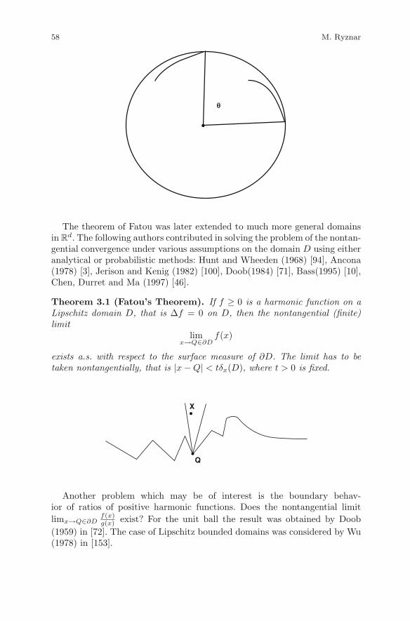
58 M. Ryznar
q
The theorem of Fatou was later extended to much more general domainsin R
d. The following authors contributed in solving the problem of the nontan-gential convergence under various assumptions on the domain D using eitheranalytical or probabilistic methods: Hunt and Wheeden (1968) [94], Ancona(1978) [3], Jerison and Kenig (1982) [100], Doob(1984) [71], Bass(1995) [10],Chen, Durret and Ma (1997) [46].
Theorem 3.1 (Fatou’s Theorem). If f ≥ 0 is a harmonic function on aLipschitz domain D, that is Δf = 0 on D, then the nontangential (finite)limit
limx→Q∈∂D
f(x)
exists a.s. with respect to the surface measure of ∂D. The limit has to betaken nontangentially, that is |x−Q| < tδx(D), where t > 0 is fixed.
Q
X
Another problem which may be of interest is the boundary behav-ior of ratios of positive harmonic functions. Does the nontangential limitlimx→Q∈∂D
f(x)g(x) exist? For the unit ball the result was obtained by Doob
(1959) in [72]. The case of Lipschitz bounded domains was considered by Wu(1978) in [153].
3 Nontangential Convergence for α-harmonic Functions 59
Theorem 3.2 (Relative Fatou’s Theorem). If f, g ≥ 0 are harmonicfunctions on a Lipschitz domain D, that is Δf = 0 on D, having the Martinrepresentation f(x) =
∫∂D
MD(x, z)μ(dz), g(x) =∫
∂DMD(x, z)ν(dz), where
MD(x, z) is the Martin kernel of D and μ, ν are finite positive measures on∂D. Then the nontangential (finite) limit
limx→Q∈∂D
f(x)g(x)
exists a.s. with respect to the measure ν.
A natural question arises if both Fatou’s theorems could be proved forα-harmonic function, 0 < α < 2 (for the definition see the next section).
The following example exhibits that the behavior of the α-harmonic func-tions, α < 2, is less regular than in the classical case.
Example 3.3. Let α < 2. Suppose that D is the open unit ball in Rd. Then
the functionf(x) = (1− |x|2)α/2−1, |x| < 1
f(x) = 0, |x| ≥ 1
is α-harmonic in D and
limx→Q∈∂D
f(x) = ∞.
Bass and You (2003) in [15] provide examples of positive bounded α-harmonic functions on a half-space such that the nontangential limit doesnot exist at almost all points of the boundary. They also gave some sufficientconditions for the nontangential convergence.
There are probabilistic proofs of the Fatou theorem taking the advantageof the fact that for harmonic f ≥ 0 and a Brownian motion Wt,
Mt = f(Wt∧τD)
is a positive supermartingale and Wt∧τDhits the boundary at the exiting
time τD.Let us remark that for the α-stable process, α < 2, due to its jumping
nature, this argument can not be applied. Nevertheless it turns out that therelative Fatou theorem for α-harmonic functions holds at least for some pointsof the boundary but we need to impose some further assumptions on thefunctions (see Theorem 3.4). Namely we need to consider so called singularα-harmonic functions, which are precisely defined in the next section.

60 M. Ryznar
3.2 Basic Definitions and Properties
We assume that (Xt, Px) is a rotation invariant (isotropic) α-stable Levy mo-
tion on Rd, d ≥ 2 with index α ∈ (0, 2). That is it has independent stationary
increments and its characteristic function is given by the following formula:
E0eiz·Xt = e−t|z|α , z ∈ Rd.
For an open set D ⊂ Rd we define its first exit time τD = inf{t � 0 : Xt /∈
D}. One of the basic objects in the potential theory of the stable process isthe so-called α-harmonic measure of D given by
ωxD(B) = P x(XτD
∈ B), B ⊂ Dc, x ∈ Rd.
Recall that an open D is a Lipschitz set if there exist constants R0 (local-ization radius) and λ > 0 (Lipschitz constant) such that for every Q ∈ ∂Dthere is a function F : R
d−1 → R and an orthonormal coordinate systemy = (y1, ..., yd) such that
D ∩B(Q,R0) = {y : yd > F (y1, ..., yd−1)} ∩B(Q,R0).
Moreover F is Lipschitz with the Lipschitz constant not greater than λ.If F is differentiable and ∇F is Lipschitz with the Lipschitz constant not
greater than λ then D is called a C1,1 set.
Fig. 3.1 TypicalLipschitz domain
R0
Q

3 Nontangential Convergence for α-harmonic Functions 61
If D is a bounded Lipschitz set then ωxD(∂D) = 0 and ωx
D has the densitywith respect to the Lebesgue measure called the Poisson kernel of D,
PD(x, y), x ∈ D, y ∈ (D)c.
When D = B(0, r), r > 0, the Poisson kernel is given by an explicitformula:
Pr(x, y) = Cd,α
(r2 − |x|2|y|2 − r2
)α/2 1|x− y|d , |x| < r, |y| > r,
where Cd,α = Γ(d/2)π−d/2−1 sin(πα/2) (see [25]).A Borel function h on R
d is said to be α-harmonic on D if for each boundedopen set B with B ⊂ D and for x ∈ B we have
h(x) = Exh(XτB),
where the last integral is absolutely convergent. If h ≡ 0 on Dc then it iscalled singular α-harmonic on D. On the other hand h is called regularα-harmonic on D if
h(x) = Exh(XτD).
For example the harmonic measure ωxD(B) for a fixed B is regular α-harmonic
on D as a function of x.We define the Riesz potential by the formula
U(x− y) =∫ ∞
0
pt(x− y)dt = Ad,α|x− y|α−d,
where pt(x − y) is the transition density of the process Xt and Ad,α is apositive constant dependent on d, α.
The Green function of D is defined as
GD(x, y) = Ad,−α(|x− y|α−d − Ex|y −XτD|α−d), x, y ∈ D,x �= y.
A very important result in the potential theory of the stable process is
Boundary Harnack Principle (BHP). Let D be a Lipschitz domain andU an open subset of R
d, K a compact subset of U such that K ∩ D �= ∅.There exists co ∈ (0,∞) such that for every u, v � 0, α-harmonic in D andvanishing continuously on Dc ∩ U , with u(x0) = v(x0) for fixed x0 ∈ K wehave
cov(y) � u(y) � c−1o v(y) ,
for all y ∈ K ∩D.
This result was proved by Bogdan [27]. See also [150].

62 M. Ryznar
Another important object of the potential theory is the so-called Martinkernel. It may be defined as the following limit, which exists due to BHP:
M(x, z) = limDy→z
GD(x, y)GD(x0, y)
, x ∈ D, z ∈ ∂D,
where x0 ∈ D is a reference point chosen at our convenience.Every nonnegative singular α-harmonic function on D has a unique rep-
resentation called the Martin representation. That is
f(x) =∫
∂D
M(x, z)μ(dz),
where μ is a finite measure on ∂D (see Chen and Song (1998) [50] or Bogdan(1999)[28]).
For the unit ball and x0 = 0:
M(x, z) =(1− |x|2)α/2
|x− z|d , |x| < 1; |z| = 1.
Let us observe that taking the uniform measure on the unit sphere onecan easily show that the function
f(x) = (1− |x|2)α/2−1, |x| < 1; f(x) = 0, |x| ≥ 1,
is an example of a singular α-harmonic function on the unit ball. Recall thatthis is the function from Example 3.3.
3.3 Relative Fatou Theorem for α-Harmonic Functions
Throughout the whole section we assume that D is a Lipschitz bounded setunless stated otherwise. Suppose that u(x), v(x) are two nonnegative singularα-harmonic functions, 0 < α < 2, determined by two Borel finite measuresconcentrated on ∂D. That is
u(x) =∫
∂D
M(x, z)μ(dz), v(x) =∫
∂D
M(x, z)ν(dz).
Next we can write the following decomposition of the measure μ(dz):
dμ = fdν + dμs,
where μs is singular to ν and f ∈ L1(ν) is a positive function.The first result about the boundary limit behavior of the ratio of u(x) and
v(x) was obtained by Bogdan and Dyda (2003) in [34] for the special casedμ = fdσ, where σ is the Haussdorff surface measure concentrated on ∂D for

3 Nontangential Convergence for α-harmonic Functions 63
a bounded C1,1 open set. They showed that for σ-almost every point Q ∈ ∂Dwe have
limx→Q
u(x)v(x)
= f(Q),
provided that the limit is taken nontangentially. Then that result was gener-alized independently to the general setting for Lipschitz sets by Michalik andRyznar 2004 [124] and Kim (2006) [101]. As a matter of fact Kim in [101]studied even more general sets than Lipschitz: namely he considered so calledκ-fat sets (see Remark 3.5 below)
Theorem 3.4. For ν-almost every point Q ∈ ∂D we have
limx→Q
u(x)v(x)
= f(Q)
as x→ Q nontangentially.
The methods used in [124] and [101] to prove Theorem 3.4 are different.While the proof in [124] is mostly analytical then [101] uses more probabilisticarguments. In the rest of this section we provide the outline of the proof from[124]. We start with reminding some estimates of the Martin kernel and thenwe provide the proof of the maximal estimate (see Lemma 3.6) which is themain tool in establishing Theorem 3.4.
Useful Estimates for Martin KernelThe basic estimates for M were obtained by Jakubowski (2002) in [98].
Before stating this result we need to define points AQ,r, Q ∈ ∂D, r > 0. Letx0 ∈ D be a fixed reference point. For r ≤ R0/32 we denote by AQ,r a pointfor which
B(AQ,r, κr) ⊂ B(Q, r) ∩D (3.1)
for a certain absolute constant κ = κ(D) = 1/(2√
1 + λ2). For r > R0/32we set AQ,r = x1, where x1 ∈ D is such that |x0 − x1| = R0/4. The picturebelow explains how to locate AQ,r.
Q
AQ,r
r

64 M. Ryznar
Remark 3.5. There are non-Lipschitz sets for which the property (3.1) holdswith some κ and 0 < r ≤ r0. Sets for which (3.1) holds are called κ-fat.
The above mentioned result from [98] states that
cφ(x)
|x− z|d−αφ2(Az,|x−z|)≤M(x, z) ≤ C
φ(x)|x− z|d−αφ2(Az,|x−z|)
, (3.2)
where c, C depend on d, α, λ and
φ(x) = min(GD(x, x0), Cd,α(R0/4)α−d).
If D is a C1,1 domain then Kulczycki (1997) in [109], Chen and Song (1998)in [51] showed that
cδx(D)α/2
|x− z|d ≤M(x, z) ≤ Cδx(D)α/2
|x− z|d ,
where δx(D) = dist (∂D, x).To take advantage of (3.2) one has to estimate the function φ(x). This can
be achieved by considering cones and their Martin kernels (see [5]).An unbounded circular cone with vertex at 0 = (0, 0, ..., 0) and symmetric
with respect to the d-th axis is a set Γ defined as
Γ = {x : η · |(x1, x2, ..., xd−1)| < xd},
where η ∈ (−∞,∞), see Figure 3.2 below. The aperture of Γ is the angleγ = arccos(η/
√1 + η2) ∈ (0, π).
Let Γ be a cone with vertex at 0 and aperture γ ∈ (0, π). Assume that1 = (0, 0, ..., 0, 1). From Bogdan and Banuelos (2003) [5] there exists a uniquenonnegative function MΓ on R
d the Martin kernel with pole at infinity calledsuch that MΓ(1) = 1, MΓ ≡ 0 on Γc and MΓ is regular α-harmonic onevery open bounded subset of Γ. Moreover, MΓ is locally bounded on R
d andhomogeneous of degree β ∈ [0, α), that is,
MΓ(x) = |x|βMΓ(x/|x|), x ∈ Γ.
Furthermore, β = β(Γ, α) called the characteristic of Γ is a strictly decreasingfunction of γ. An exact relationship between the aperture and the charac-teristic of Γ is not well known except a few cases including γ = π/2, that iswhen Γ is a half-space. In this case MΓ(x) = x
α/2d , x ∈ Γ, so β = α/2.
For a cone Γ with vertex at Q (obviously isometric to some cone withvertex at 0) we define a bounded cone Γr = Γ∩B(Q, r). For any Q ∈ ∂D, bythe properties of Lipschitz sets we know that there exists R0 > 0 such thatfor every r ≤ R0 there exist cones Γ, Γ such that

3 Nontangential Convergence for α-harmonic Functions 65
0
1
g
Fig. 3.2 Bounded and unbounded circular cones
Q
Fig. 3.3 Inner cone and covering cone
Γr ⊂ D ∩B(Q,R0) ⊂ Γr.
Here β, β may depend locally on Γ, r. We will call Γr an inner bounded coneand Γr a covering bounded cone (see Figure 3.3).
There are r0 and β0, β0 such that cones with characteristic β0 ≥ β0, re-spectively, are universal for every boundary point:
B(AQ,r0 , κr0) ⊂ Γr0 ⊂ Γr0

66 M. Ryznar
andΓr0 ⊂ B(Q, r0) ∩D ⊂ Γr0 .
These observations enable a comparison between the function φ and the Mar-tin kernels of the inner bounded cone or the covering bounded cone locallyat the vicinity of Q or globally if we use cones with characteristics β0 ≥ β0.The Boundary Harnack Principle together with optimal estimates of Martinkernels for cones (see [123]) give tools to get useful estimates for the Martinkernel M(x, z) of D. For the proofs of following Lemmas 3.6, 3.8 and 3.9 see[124].
Lemma 3.6. Let r ≤ R0. For Q ∈ ∂D consider an inner bounded coneΓr and a covering bounded cone Γr with characteristics β, β . Moreover, let|x − Q| ≤ |x − z|. Then there exist constants c = c(r,D, β, β) and C =C(r,D, β, β) such that
c
(|x−Q||x− z|
)d−α+2β
≤ M(x, z)M(x,Q)
≤ C
(|x−Q||x− z|
)d−α+2β
.
Corollary 3.7. Let z, z′ ∈ ∂D, x ∈ D and |x − z′| ≤ |x − z| . There areuniversal β0 ≥ β0 both smaller than α such that there exist constants c =c(R0,D, β0, β0) and C = C(R0,D, β0, β0) such that
c
(|x− z′||x− z|
)d−α+2β0
≤ M(x, z)M(x, z′)
≤ C
(|x− z′||x− z|
)d−α+2β0
.
Lemma 3.8. Let r ≤ R0. For Q ∈ ∂D consider an inner bounded cone Γr
and a covering bounded cone Γr. Moreover, let |z−Q| ≤ 2|x− z|. Then thereexist constants c = c(r,D, β, β) and C = C(r,D, β, β) such that
cφ(x)
|x− z|d−α+2β≤M(x, z) ≤ C
φ(x)|x− z|d−α+2β
.
Furthermore, if β = β0 and β = β0 then c = c(R0,D, β0, β0) and C =C(R0,D, β0, β0). In this case the above estimates hold for all z ∈ ∂D, x ∈ D.
Lemma 3.9. If v(x) =∫
∂DM(x, z)ν(dz) then
lim infx→Q
v(x) > 0
for ν almost all Q provided the limit is nontangential.
As an immediate consequence of the above lemma and the well known fact
GD(x, x0) → 0 if x→ Q
3 Nontangential Convergence for α-harmonic Functions 67
we have that
GD(x, x0)v(x)
→ 0 as x→ Q (3.3)
for ν almost all Q provided the limit is nontangential.Now we can easily show that if dμ = fdν and f is continuous at Q then
the ratio of u and v converges to f for all such points Q that (3.3) holds. Tosee this we define
I1(x) =∫
∂D∩{|z−Q|≥ε}|f(z)− f(Q)|M(x, z)ν(dz),
I2(x) =∫
∂D∩{|z−Q|<ε}|f(z)− f(Q)|M(x, z)ν(dz).
and then
∣∣∣∣u(x)v(x)
− f(Q)∣∣∣∣ ≤∫
∂D|f(z)− f(Q)|M(x, z)ν(dz)
v(x)
=I1(x)v(x)
+I2(x)v(x)
.
At first we estimate the term I1(x)v(x) . By Lemma 3.4,
M(x, z) ≤ Cφ(x)
|x− z|d−α+2β0≤ C
GD(x, x0)|x− z|d−α+2β0
.
If |z −Q| ≥ ε and |x−Q| ≤ ε/2 then |x− z| ≥ ε/2. This implies
M(x, z) ≤ C(ε)GD(x, x0).
Hence
I1(x) =∫
∂D∩{|z−Q|≥ε}|f(z)− f(Q)|M(x, z)ν(dz)
≤ C(ε)|μ|GD(x, x0)∫
∂D
|f(z)− f(Q)|ν(dz),
which together with (3.3) shows that
I1(x)v(x)
→ 0, as x→ Q. (3.4)
Observe that the above limit holds without the continuity assumption.

68 M. Ryznar
Next, note that
I2(x) ≤ sup|z−Q|≤ε
|f(z)− f(Q)|v(x)
henceI2(x)v(x)
≤ sup|z−Q|≤ε
|f(z)− f(Q)| → 0, as ε→ 0
by the continuity of f at Q.To provide the proof of the relative Fatou theorem in the general case we
need the following crucial lemma.
Lemma 3.10 (Nontangential Maximal Estimate). Suppose that
u(x) =∫
∂D
M(x, z)μ(dz), v(x) =∫
∂D
M(x, z)ν(dz).
For any x ∈ D, Q ∈ ∂D and t > 0 such that |x − Q| ≤ tδx(D) there existconstants C = C(t,Q), c = c(t,Q) such that
u(x)v(x)
≤ C supr>0
μ(B(Q, r))ν(B(Q, r))
.
Proof. For n ≥ 1 setBn = B(Q, 2n|x−Q|)
andA1 = B1, An = Bn \Bn−1, n ≥ 2.
x
zA2 A1 Q
If z ∈ A1 then
|x−Q|/t ≤ δx ≤ |x− z| ≤ 3|x−Q|.

3 Nontangential Convergence for α-harmonic Functions 69
If z ∈ An then
(2n−1 − 1)|x−Q| ≤ |x− z| ≤ (2n + 1)|x−Q|.
Define an = supz∈AnM(x, z), z ∈ An and observe that by Lemma 3.2
an ≈ M(x, z), z ∈ An.
If z′ ∈ An and z ∈ Ak, k > n then
|x− z′| ≤ 4|x− z|.
Hence by Lemma 3.2 we obtain
M(x, z) ≤ CM(x, z′)
for some C ≥ 1 dependent on t and Q. It implies that ak ≤ Can for k > nand for
bn = supk≥n
ak, n ≥ 1,
this yieldsan ≤ bn ≤ Can.
Then we obtain
u(x) =∫
∂D
M(x, z)μ(dz) =n0∑
n=1
∫An
M(x, z)μ(dz)
≈n0∑
n=1
anμ(An)
≈n0∑
n=1
bnμ(An),
where n0 be the smallest index for which 2n0 |x−Q| ≥ diam(D). Denote
R = supr>0
μ(B(Q, r))ν(B(Q, r))
Now summation by parts yields (note that bn is nonincreasing):
u(x) ≈n0∑
n=1
bnμ(An) =
=n0∑
n=2
(bn−1 − bn)μ(Bn)ν(Bn)
ν(Bn) + bn0
μ(Bn0)ν(Bn0)
ν(Bn0)

70 M. Ryznar
≤ R
(n0∑
n=2
(bn−1 − bn)ν(Bn) + bn0ν(Bn0)
)
= R
n0∑n=1
bnν(An)
≈ Rv(x). ��
Now we can complete the proof of Theorem 3.4. Let μ(dz) = |f(z) −f(Q)|ν(dz) + μs(dz). Then
∣∣∣∣u(x)v(x)
− f(Q)∣∣∣∣ ≤∫
∂D
M(x, z)μ(dz)/v(x)
≤∫
∂D∩{|z−Q|≥ε}M(x, z)μ(dz)/v(x)
+∫
∂D∩{|z−Q|<ε}M(x, z)μ(dz)/v(x).
The first term converges to 0, by the same argument as leading to (3.4),if x → Q and (3.3) holds. To take care of the second term we apply theMaximal Inequality to arrive at
∫∂D∩{|z−Q|<ε}
M(x, z)μ(dz)/v(x)
≤ C
(supr≤ε
∫∂D∩B(Q,r)
|f(z)− f(Q)|ν(dz)
ν(B(Q, r))+ sup
r≤ε
μs(B(Q, r))ν(B(Q, r))
)
Next, observe that the set of points Q for which the limit
limε→0
(supr≤ε
∫∂D∩B(Q,r)
|f(z)− f(Q)|ν(dz)
ν(B(Q, r))+ sup
r≤ε
μs(B(Q, r))ν(B(Q, r))
)�= 0 (3.5)
is of ν measure zero. This completes the sketch of the proof of Theorem 3.4.Note that the advantage of the above proof is that we can identify the
points Q ∈ ∂D for which the ratio converges. Namely these are points forwhich (3.3) and (3.5) hold.
3.4 Extensions to Other Processes
At first we consider the relativistic α-stable process 0 < α < 2. This is a Levyprocess which characteristic function is of the form
E0eiz·Yt = e−t((|z|2+m2/α)α/2−m), z ∈ Rd,

3 Nontangential Convergence for α-harmonic Functions 71
where m > 0 is a parameter (see also Example 5.9 below). For m = 0 itreduces to the isotropic α-stable process. The generator of this process isgiven by
Am = m−(−Δ + m2/α
)α/2
.
To explain the name relativistic observe that if α = 1 the generator is relatedto the kinetic energy of the relativistic particle of mass m, see [45]. If νY isthe Levy measure of Yt and νX is the Levy measure of Xt (isotropic stable)then (see [134]) νX − νY is a finite positive measure, which is equivalent tothe fact that Am − A0 is a bounded operator. It suggests that the potentialtheory of such a process should bear a lot of similarity with the potentialtheory of the stable process. This is the case if we study properties of theprocess killed after exiting a bounded open set.
Theorem 3.11 (Green Function Estimates). Let D be an open Lips-chitz bounded set. There is a positive constant C = C(D) such that
C−1GXD(x, y) ≤ GY
D(x, y) ≤ CGXD(x, y), x, y ∈ D, (3.6)
where GXD , GY
D are corresponding Green functions of D.
Remark 3.12. The comparison above may not hold for unbounded sets. Inthe paper [83] optimal estimates for the Green function of a half-space arederived and they exhibit that the Green function is comparable to the Brown-ian Green function for the points away from the boundary and not too closeto each other.
For a bounded open C1,1 set D the comparison (3.6) was proved by Ryznar(2002) [134] and by another method by Chen and Song (2003) [53]. Later onthat result was proved for bounded open Lipschitz sets by Grzywny, Ryznar(2006) [82] and for κ-fat sets by Kim and Lee (2006) [102].
This estimate plus some other properties of the Levy measure of Y willallow to study potential theory for the relativistic process very much thesame as for the stable process provided that D is bounded and Lipschitz. Forexample one can prove the existence of the Martin kernel of D for the processY and show that relative Fatou’s theorem holds for nonnegative functionsdefined by the Martin kernel MY
D (x, z):
h(x) =∫
∂D
MYD (x, z)μ(dz).
Such a result for example was proved in [101] and [102], where a class ofnonlocal Feynman-Kac transforms of the stable process was studied. Therelativistic stable process is included in this class. It is easy to see that theproof presented in the previous section will go through in the relativistic casesince due to Theorem 3.11 we are able to derive all needed estimates for theMartin kernel of Y .

72 M. Ryznar
Theorem 4.1 suggests that we should expect a similar result if we takeas Yt any Levy process with its Levy measure sufficiently close to the Levymeasure νX . Let
E0eiz·Yt = e−t∫
Rd (1−cos(z·w))νY (dw),
where νY is the Levy measure of Yt and we assume that
νY − νX is a finite signed measure.
Question. Is there a positive constant C such that
C−1GXD(x, y) ≤ GY
D(x, y) ≤ CGXD(x, y), x, y ∈ D?
Theorem 3.13. Suppose that D is an open bounded set. If νX ≥ νY then
GYD(x, y) ≤ CGX
D(x, y).
If νX ≤ νY thenGX
D(x, y) ≤ CGYD(x, y)
This result was proved by Grzywny and Ryznar (2006) in [82]. Under theadditional assumption about the densities νX(x), νY (x) of the correspondingLevy measures:
|νX(x)− νY (x)| ≤ C|x|−d+�, |x| ≤ 1, � > 0,
the answer for the raised question is positive but we need to assume that Dis bounded Lipschitz and connected (see [82]). Namely there is a constant Csuch that
C−1GXD(x, y) ≤ GY
D(x, y) ≤ CGXD(x, y), x, y ∈ D.
The assumption that D is connected is not to avoid, since the Levy measureνY can be concentrated on some neighborhood of the origin so the processcan only make small jumps, so GD(x, y) might be 0 if D has components faraway from each other. This will not happen for the stable case.
For open bounded κ-fat sets the result can be deduced under some ad-ditional assumptions on the behavior of the Levy measure at ∞ from theresults of Kim and Lee (2006) [102].
The comparability of the Green functions allows to prove many propertiessimilar to those possessed by the stable process. Again we can expect therelative Fatou theorem holds however some further assumptions are necessary.For example for the truncated stable process, that is if νY = νX |B(0,R), R >0, the relative Fatou theorem is true for connected bounded κ - fat sets. Thisis a recent result obtained by Kim and Song in [104](see also [103]).
Chapter 4
Eigenvalues and Eigenfunctions for StableProcesses
by T. Kulczycki
4.1 Introduction
Let Xt be a symmetric α-stable process in Rd, α ∈ (0, 2]. This is a process with
independent and stationary increments and characteristic function E0eiξXt =e−t|ξ|α , ξ ∈ R
d, t > 0. We will use Ex, P x to denote the expectation andprobability of this process starting at x, respectively. By p(t, x, y) = pt(x−y)we will denote the transition density of this process. That is,
P x(Xt ∈ B) =∫
B
p(t, x, y) dy.
When α = 2 the process Xt is just the Brownian motion in Rd running at
twice the speed. That is, if α = 2 then
p(2)(t, x, y) =1
(4πt)d/2e
−|x−y|24t , t > 0, x, y ∈ R
d. (4.1)
When α = 1, the process Xt is the Cauchy process in Rd whose transition
densities are given by
p(1)(t, x, y) =cd t
(t2 + |x− y|2)(d+1)/2, t > 0, x, y ∈ R
d, (4.2)
wherecd = Γ((d + 1)/2)/π(d+1)/2.
We are mainly interested in the eigenvalues and eigenfunctions of thesemigroup {PD
t }t≥0 of the process Xt killed upon exiting a domain D ⊂ Rd.
Let D ⊂ Rd be a domain with finite Lebesgue measure m(D) < ∞ and
τD = inf{t ≥ 0 : Xt /∈ D}
K. Bogdan et al., Potential Analysis of Stable Processes and its Extensions,Lecture Notes in Mathematics 1980, DOI 10.1007/978-3-642-02141-1 4,c© Springer-Verlag Berlin Heidelberg 2009
73

74 T. Kulczycki
be the first exit time of D. By {PDt }t≥0 we denote the semigroup on L2(D)
of Xt killed upon exiting D. That is,
PDt f(x) = Ex(f(Xt), τD > t), x ∈ D, t > 0, f ∈ L2(D).
The semigroup has transition densities pD(t, x, y) satisfying
PDt f(x) =
∫D
pD(t, x, y)f(y) dy.
The kernel pD(t, x, y) is strictly positive symmetric and
pD(t, x, y) ≤ p(t, x, y) ≤ cα,d t−d/α, x, y ∈ D, t > 0.
It follows that∫
D
∫D
p2D(t, x, y) dx dy ≤ c2
α,d t−2d/αm(D)2 < ∞
so for any t > 0 the operator PDt is a Hilbert-Schmidt operator. Hence for
any t > 0 the operator PDt is compact. From the general theory of semigroups
it follows that there exists an orthonormal basis of eigenfunctions {ϕn}∞n=1
for L2(D) and corresponding eigenvalues {λn}∞n=1 satisfying
0 < λ1 < λ2 � λ3 � . . .
with λn →∞ as n →∞. That is, the pair {ϕn, λn} satisfies
PDt ϕn(x) = e−λntϕn(x), x ∈ D, t > 0. (4.3)
We also have
pD(t, x, y) =∞∑
n=1
e−λntϕn(x)ϕn(y).
The eigenfunctions ϕn are continuous and bounded on D. In addition, λ1
is simple and the corresponding eigenfunction ϕ1, often called the groundstate eigenfunction, is strictly positive on D. For more general properties ofthe semigroups {PD
t }t≥0, see [79], [24], [54].Let A be the infinitesimal generator of the semigroup {PD
t }t≥0. We have
Aϕn(x) = limt→0
PDt ϕn(x)− ϕn(x)
t
= limt→0
e−λnt − 1t
ϕn(x)
= −λnϕn(x).
4 Eigenvalues and Eigenfunctions for Stable Processes 75
For any t > 0 we also have
|ϕn(x)| = eλnt
∣∣∣∣∫
D
pD(t, x, y)ϕn(y) dy
∣∣∣∣≤ eλnt||ϕn||∞
∫D
pD(t, x, y) dy
= eλnt||ϕn||∞P x(τD > t) → 0,
when x → x0 ∈ ∂D and x0 is a regular point. We say that x0 ∈ ∂D is aregular point when P x
0 (τD = 0) = 1. It may be shown that if D satisfies theouter cone condition at x0 ∈ ∂D then x0 is regular.
It follows that if all points on ∂D are regular we have
⎧⎨⎩Aϕn(x) = −λn(x), x ∈ D
ϕn(x) = 0, x ∈ ∂D.
When α = 2 and Xt is Brownian motion the semigroup {PDt }t≥0 is just
the heat semigroup. Eigenvalues and eigenfunctions are the solutions of theeigenvalue problem for the Dirichlet Laplacian :
⎧⎨⎩
Δϕn(x) = −λn(x), x ∈ D
ϕn(x) = 0, x ∈ ∂D.
For example when D = (0, π)
ϕn(x) =√
2/π sin(nx), λn = n2.
Indeedsin′′(nx) = −n2 sin(nx), sin(0) = sin(nπ) = 0.
In particular the first eigenfunction is strictly positive on D = (0, π)
ϕ1(x) =√
2/π sin(x).
The second eigenfunction changes the sign once on D = (0, π)
ϕ2(x) =√
2/π sin(2x).
Let us observe that eigenfunctions in this example satisfy the followingproperty: nth eigenfunction ϕn has exactly n nodal domains. A nodal domainfor an eigenfunction ϕ is any connected component of a set on which ϕ hasa constant sign.

76 T. Kulczycki
In general, the eigenfunctions of the eigenvalue problem for the DirichletLaplacian satisfies the Courant-Hilbert nodal domain theorem, which statesthat the n-th eigenfunction has no more than n nodal domains.
When α ∈ (0, 2) eigenfunctions and eigenvalues satisfy
⎧⎨⎩−(−Δ)α/2ϕn(x) = −λn(x), x ∈ D
ϕn(x) = 0, x ∈ Dc,(4.4)
where
−(−Δ)α/2f(x) = limε↓0Ad,−α
∫|x−y|>ε
f(y)− f(x)|y − x|d+α
dy.
with Ad,γ = Γ((d − γ)/2)/(2γπd/2|Γ(γ/2)|). Nevertheless, in the case α ∈(0, 2) the operator −(−Δ)α/2 is a pseudodifferential nonlocal operator andit is very difficult to obtain some properties of the semigroup and its eigen-functions and eigenvalues using equations (4.4).
4.2 Intrinsic Ultracontractivity (IU)
Intrinsic ultracontractivity is the property of the semigroup which is veryuseful in studying spectral properties of the eigenvalues and eigenfunctionscf. [6].
Definition 4.1. The semigroup {PDt }t≥0 is intrinsically ultracontractive
(IU) when for any t > 0 there exists ct such that for any x, y ∈ D wehave
∀t > 0 ∃ct < ∞ ∀x, y ∈ D pD(t, x, y) ≤ ctϕ1(x)ϕ1(y).
There are many other well known equivalent definitions of IU. We presentprobabilistic definition of IU which will be very useful in studying semigroupsfor stable processes.
Proposition 4.1. The semigroup {PDt }t≥0 is IU if and only if
∃K ⊂⊂ D ∀t > 0 ∃c = ct,K,D ∀x ∈ D P x(τD > t) ≤ cP x(τD > t,Xt ∈ K).
The following very important result is proved in [110].
Theorem 4.2. When α ∈ (0, 2) and D ⊂ Rd is bounded then {PD
t }t≥0
is IU.
Proof. (idea) Let us fix K = B(x0, r) such that K ⊂ D and let us denoteK1 = B(x0, r/2). We will use c to denote positive constant which depend ont > 0, d, D, K and α. This constant may change its value from line to line.We have for x ∈ D

4 Eigenvalues and Eigenfunctions for Stable Processes 77
P x(τD > t,Xt ∈ K)≥ P x(τD\K1 < t,X(τD\K1) ∈ K1,Xs in K for all s ∈ (τD\K1 , τD\K1 + t))≥ cP x(τD\K1 < t,X(τD\K1) ∈ K1).
By the Ikeda-Watanabe formula ([96]) it equals for x ∈ D \K1
c
∫D
∫ t
0
pD\K1(s, x, y) dsAd,−α
|y − z|d+αdy dz.
We have |y − z|−d−α ≥ (diam(D))−d−α so the above expression is boundedbelow by
c
∫D
∫ t
0
pD\K1(s, x, y) dy ds
≥ c
∫ t
0
P x(τD\K1 > s) ds
≥ ctP x(τD\K1 > t).
It follows that for x ∈ D
P x(τD > t) ≤ P x(τD\K1 ≥ t) + P x(τD\K1 < t,X(τD\K1) ∈ K1)≤ cP x(τD > t,Xt ∈ K). ��
We havepD(t, x, y) =
∫ ∞
0
e−λntϕn(x)ϕn(y).
It follows that
pD(t, x, y)e−λ1tϕ1(x)ϕ1(y)
= 1 +∞∑
n=2
e−(λn−λ1)tϕn(x)ϕn(y)ϕ1(x)ϕ1(y)
.
Proposition 4.3 (Consequences of IU). Let α ∈ (0, 2) and D ⊂ Rd is a
bounded open set. Theni)
limt→∞
pD(t, x, y)e−λ1tϕ1(x)ϕ1(y)
= 1.
ii) ∃C = C(D,α) ∀t ≥ 1
e−(λ2−λ1)t ≤ supx,y∈D
∣∣∣∣ pD(t, x, y)e−λ1tϕ1(x)ϕ1(y)
∣∣∣∣ ≤ Ce−(λ2−λ1)t
The next theorem proved in [110] gives asymptotic of ϕ1.
78 T. Kulczycki
Theorem 4.4. Let α ∈ (0, 2) and D ⊂ Rd is a bounded open set. Then there
exist constants C1 = C1(D,α), C2 = C2(D,α) such that for all x ∈ D
C1Ex(τD) ≤ ϕ1(x) ≤ C2E
x(τD).
This theorem implies that for α ∈ (0, 2) when D = B(0, r) is a ball in Rd
we haveϕ1(x) ≈ Ex(τD) = cα,d(r2 − |x|2)α/2,
when D = B(0, r) is a ball in Rd,
ϕ1(x) ≈ Ex(τD) ≈ δα/2D (x),
when D is a bounded C1,1 domain (δD(x) = dist(x, ∂D)),
c1δγ1D (x) ≤ ϕ1(x) ≤ c2δ
γ2D (x),
when D is a bounded Lipschitz domain, c1, c2, γ1, γ2 > 0 depend on D and α.Intrinsic ultracontractivity may be investigated for some other semigroups
e.g. Feynman-Kac semigroups in Rd with Schrodinger generators H0 − V
where V : Rd → R is a potential. Recently the following result has been
obtained for relativistic α-stable processes. The relativistic α-stable processin R
d is a Markov process with independent and homogeneous incrementsand the characteristic function of the form
E0(exp(iξXt)) = exp(−t((m2/α + |ξ|2)α/2 −m)
),
m > 0.The following result was proved in [112].
Theorem 4.5. Let α ∈ (0, 2), d > α. Let Xt be a relativistic α-stable pro-cess and {Tt}t≥0 a Feynman-Kac semigroup for Xt with generator −((−Δ+m2/α)α/2−m)− V , where potential V (x) = |x|β, β > 0. We have
i) Tt are compact for any β > 0,ii) {Tt}t≥0 is IU if and only if β > 1,iii) for β > 1
ϕ1(x) ≈ exp(−m1/α|x|)(|x|+ 1)(d+α+2β+1)/2
.
4.3 Steklov Problem
IU gives some general properties of the first and consecutive eigenfunctionsfor the semigroup of symmetric α-stable processes. Nevertheless we do notknow many fine properties of eigenvalues and eigenfunctions which are known

4 Eigenvalues and Eigenfunctions for Stable Processes 79
for eigenvalues and eigenfunctions of Dirichlet Laplacian (α ∈ (0, 2)). Evenin the most simple geometric case when D = (−1, 1) we do not know almostany properties.
A very simple question is the following. What can be said about the secondeigenfunction ϕ2? How many zeroes has this function on (−1, 1)?
Some answers were obtained for the Cauchy process (symmetric α-stableprocess for α = 1). This was done in [7] by using the connection of thespectral problem for this process and the Steklov problem.
The connection between the eigenvalue problem for the Cauchy processand the Steklov problem arises as follows.
Let us consider the following construction. Let D = (−1, 1) and ϕn, λn
be eigenvalues and eigenfunctions for the semigroup of the Cauchy process(i.e. α-stable process for α = 1) killed on exiting D. ϕn are defined on D butlet us defined them on R by putting ϕn(x) = 0 for x ∈ Dc. Since |ϕn(x)| ≤cnϕ1(x) ≈ (1− |x|2)1/2 on D we get that ϕn is continuous on R.
LetH = {(x, t) : x ∈ R
d, t ≥ 0}be the upper half-space. Let us also denote H+ = {(x, t) : x ∈ R
d, t > 0}.We define functions un(x, t) for (x, t) ∈ H in the following way. For t = 0 weput un(x, 0) = ϕn(x). For t > 0 we put
un(x, t) =∫
Rd
p(t, x, y)ϕn(y) dy,
where p(t, x, y) is the transition density for the Cauchy process (α-stableprocess for α = 1). Let us recall that
p(t, x, y) =1π
t
t2 + (x− y)2, t > 0, x, y ∈ R.
Since ϕn are continuous on R we obtain that un are continuous on H.A very important fact is that the transition density for the Cauchy process
p(t, x, y) is the Poisson kernel for upper half-space H for classical harmonicmeasure. More precisely p(t, x, y) is the Poisson kernel for points (y, t) ∈ H+,(x, 0) ∈ ∂H. It follows that un(x, t) is harmonic for (x, t) ∈ H+ for LaplacianΔ = ∂2
∂x2 + ∂2
∂t2 in R2.
It can also be shown that
∂un
∂t(x, 0) = −λnun(x, 0).
Heuristically it can be verified as follows
∂un
∂t(x, 0) = lim
t→0+
un(x, t)− un(x, 0)t
= limt→0+
∫Rd
p(t, x, y)(ϕn(y)− ϕn(x))t
dy

80 T. Kulczycki
= limt→0+
cd
∫Rd
ϕn(y)− ϕn(x)
(t2 + |x− y|2) d+12
dy
= −(−Δ)1/2ϕn(x)= −λnϕn(x).
The precise proof may be find in [7] (proof of Theorem 1.1).Therefore un(x, t) satisfy
Δun(x, t) = 0; (x, t) ∈ H+, (4.5)∂un
∂t(x, 0) = −λnun(x, 0); x ∈ D (4.6)
un(x, 0) = 0; x ∈ Dc. (4.7)
This problem is known as the mixed Steklov problem.Using this connection the following result has been obtained [7].
Theorem 4.6. Let α = 1, D = (−1, 1) and let ϕn, λn be eigenvalues andeigenfunctions for the semigroup of the Cauchy process (i.e. α-stable processfor α = 1) killed on exiting D. Then we have
i) 1 ≤ λ1 ≤ 1.17, ϕ1 is positive, symmetric, increasing on (−1, 0), decreas-ing on (0, 1) and concave on (−1, 1),
ii) 2 ≤ λ2 ≤ π, ϕ2 is antisymmetric and (up to a sign) negative and convexon (−1, 0), positive and concave on (0, 1),
iii) 3.4 ≤ λ3 ≤ 3π/2, ϕ3 is symmetric and has 2 zeroes on (−1, 1),iv) the spectral gap satisfies λ2 − λ1 ≥ λ1 ≥ 1,v) ϕn has no more than 2n− 2 zeroes on (−1, 1).
The Steklov problem is known for many years and belongs to classical prob-lems in spectral theory, although is less known then Dirichlet or Neumannproblems. In the famous R. Courant and D. Hilbert book [63], it appears asthe spectral problem in boundary conditions.
If Ω is a bounded domain in Rd, we write its boundary ∂Ω as the dis-
joint union of two pieces, (∂Ω)1 and (∂Ω)2, and the classical “mixed Steklov”eigenvalue problem ([88], [68], [70]) is the following mixed boundary valueproblem:
Δun(z) = 0; z ∈ Ω, (4.8)∂un
∂ν(z) = −enun(z); z ∈ (∂Ω)1. (4.9)
un(z) = 0; z ∈ (∂Ω)2, (4.10)
where Δ =∑d
i=1∂2
∂x2i
and ∂∂ν is the inner normal derivative. The basic differ-
ence between our Steklov problems and the classical one in that our domainis unbounded.
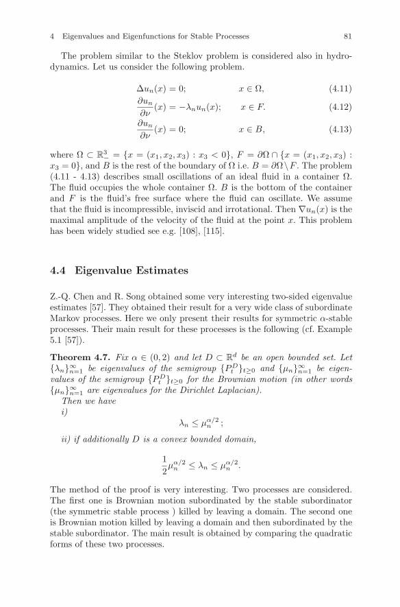
4 Eigenvalues and Eigenfunctions for Stable Processes 81
The problem similar to the Steklov problem is considered also in hydro-dynamics. Let us consider the following problem.
Δun(x) = 0; x ∈ Ω, (4.11)∂un
∂ν(x) = −λnun(x); x ∈ F. (4.12)
∂un
∂ν(x) = 0; x ∈ B, (4.13)
where Ω ⊂ R3− = {x = (x1, x2, x3) : x3 < 0}, F = ∂Ω ∩ {x = (x1, x2, x3) :
x3 = 0}, and B is the rest of the boundary of Ω i.e. B = ∂Ω\F . The problem(4.11 - 4.13) describes small oscillations of an ideal fluid in a container Ω.The fluid occupies the whole container Ω. B is the bottom of the containerand F is the fluid’s free surface where the fluid can oscillate. We assumethat the fluid is incompressible, inviscid and irrotational. Then ∇un(x) is themaximal amplitude of the velocity of the fluid at the point x. This problemhas been widely studied see e.g. [108], [115].
4.4 Eigenvalue Estimates
Z.-Q. Chen and R. Song obtained some very interesting two-sided eigenvalueestimates [57]. They obtained their result for a very wide class of subordinateMarkov processes. Here we only present their results for symmetric α-stableprocesses. Their main result for these processes is the following (cf. Example5.1 [57]).
Theorem 4.7. Fix α ∈ (0, 2) and let D ⊂ Rd be an open bounded set. Let
{λn}∞n=1 be eigenvalues of the semigroup {PDt }t≥0 and {μn}∞n=1 be eigen-
values of the semigroup {PDt }t≥0 for the Brownian motion (in other words
{μn}∞n=1 are eigenvalues for the Dirichlet Laplacian).Then we havei)
λn ≤ μα/2n ;
ii) if additionally D is a convex bounded domain,
12μα/2
n ≤ λn ≤ μα/2n .
The method of the proof is very interesting. Two processes are considered.The first one is Brownian motion subordinated by the stable subordinator(the symmetric stable process ) killed by leaving a domain. The second oneis Brownian motion killed by leaving a domain and then subordinated by thestable subordinator. The main result is obtained by comparing the quadraticforms of these two processes.

82 T. Kulczycki
4.5 Generalized Isoperimetric Inequalities
Theorem 4.8. Let us fix α ∈ (0, 2]. Let D ⊂ Rd be a bounded domain, D∗
the ball in Rd with the same volume as D. Then we have
λ1(D∗) ≤ λ1(D).
This theorem states that among all sets of equal volume the smallest firsteigenvalue has the ball. It is well known for many years.
Proof. (idea) It is well known that for any x ∈ D
λ1(D) = − limt→∞
1t
log(P x(τD > t)).
We can and do assume that 0 ∈ D and D∗ has center at 0. We have
P 0(τD > t) = limm→∞
P 0(X tm∈ D,X 2t
m∈ D, . . . ,Xmt
m∈ D, )
=∫
D
∫D
. . .
∫D
p tm
(x1)p tm
(x2 − x1) . . . p tm
(xm − xm−1) dx1 dx2 . . . dxm
≤∫
D∗
∫D∗
. . .
∫D∗
p∗tm
(x1)p∗tm
(x2 − x1) . . . p∗tm
(xm − xm−1) dx1 dx2 . . . dxm
=∫
D∗
∫D∗
. . .
∫D∗
p tm
(x1)p tm
(x2 − x1) . . . p tm
(xm − xm−1) dx1 dx2 . . . dxm.
f∗(x) denotes here a symmetric decreasing rearrangement of f(x). Since pt(x)is radial and radially decreasing we have p∗t (x) = pt(x).
It follows that
λ1(D) = − limt→∞
1t
log(P 0(τD > t))
≥ − limt→∞
1t
log(P 0(τD∗ > t))
= λ1(D∗) ��
The estimates of the spectral gap λ2 − λ1.Let α ∈ (0, 2] and D ⊂ R
d be a bounded domain. Let us recall that thereexists C(D,α) such that for all t ≥ 1 we have
e−(λ2−λ1)t ≤ supx,y∈D
∣∣∣∣ pD(t, x, y)e−λ1tϕ1(x)ϕ1(y)
− 1∣∣∣∣ ≤ C(D,α)e−(λ2−λ1)t.
In other words the spectral gap λ2 − λ1 measures the rate how quicklypD(t, x, y)/(e−λ1tϕ1(x)ϕ1(y)) tends to 1.
The spectral gap for Laplacian and Schrodinger operator has been investi-gated for many years. Motivated by problems concerning the behavior of free
4 Eigenvalues and Eigenfunctions for Stable Processes 83
Boson gases M. van den Berg made the following conjecture for all convexdomains D ⊂ R
d and convex and nonnegatives V : D → [0,∞)
λV2 − λV
1 >3π2
d2D
, (4.14)
where dD = diam(D) and λV1 , λV
2 are the first and the second eigenvalue forthe following eigenvalue problem for Schrodinger operator on D
{Δϕn(x)− V (x)ϕn(x) = −λnϕn(x); x ∈ D,
ϕn(x) = 0; x ∈ ∂D.
The case V ≡ 0 corresponds to Dirichlet Laplacian.Let us point out that for a rectangle D = (0, a)× (0, b), a > b and V ≡ 0
we have
ϕ1(x) = sin(πx1
a
)sin(πx2
b
), λ1 =
π2
a2+
π2
b2,
ϕ2(x) = sin(
2πx1
a
)sin(πx2
b
), λ2 =
4π2
a2+
π2
b2,
so the spectral gap equals λ2 − λ1 = 3π2/a2. By taking sufficiently longrectangles we can see that the estimate (4.14) is optimal.
Let us also note that for the conjecture (4.14) the assumption of convexityof D is necessary. If we take domains D with constant diameter which arenot convex then the spectral gap can be arbitrarily small. It is sufficient toconsider V ≡ 0 and the domain consisting of two disjoint balls joint togetherwith sufficiently narrow corridor.
The first substantial progress on this conjecture was made in 1985 byI. M. Singer, B. Wong, S. T. Yau and S. S. T. Yau [141], who used a maximumprinciple technique to show that
λV2 − λV
1 ≥π2
4d2D
.
Later Q. Yu i J. Q. Zhong in 1986 [157] showed that
λV2 − λV
1 ≥π2
d2D
.
Next in 1993 J. Ling [119] obtained the strict inequality
λV2 − λV
1 >π2
d2D
.

84 T. Kulczycki
In 2000 B. Davis [68] and independently R. Banuelos and P. Mendez [9]showed that if D ⊂ R
2 is convex and double symmetric (that is symmetricaccording to both coordinate axes) and V ≡ 0 then conjecture (4.14) holds i.e.
λV2 − λV
1 >3π2
d2D
.
Most (but not all) of the methods of estimating the spectral gap forLaplacian and Schrodinger operator uses the fact that the first eigenfunctionon a convex domain with a convex potential is logconcave.
Unfortunately for α ∈ (0, 2) we do not know whether the first eigenfunctionis logconcave on a convex domain. For α ∈ (0, 2) even the weaker propertythat the first eigenfunction is unimodal would be very interesting and helpfulto estimate the spectral gap. Therefore we have the following open problem.
Conjecture 4.9. Let α ∈ (0, 2) and D ⊂ Rd be a convex bounded domain.
Then the first eigenfunction ϕ1 for the semigroup {PDt }t≥0 is unimodal, that
is ϕ1 is unimodal along any line segment in D.
Of course for α = 2 the first eigenfunction ϕ1 is unimodal because islogconcave.
Even though we do not know whether the first eigenfunction is unimodalfor α ∈ (0, 2) some estimates of the spectral gap were obtained. First theywere obtained for the Cauchy process (α = 1) using the connection with theSteklov problem. Later these results were extended for all α ∈ (0, 2).
The result for the Cauchy process is the following [8].
Theorem 4.10. Let D ⊂ R2 be a bounded convex domain which is symmet-
ric relative to both coordinate axes. Assume that [−a, a]× [−b, b], a ≥ b > 0 isthe smallest rectangle (with sides parallel to the coordinate axes) containingD. Let {λn}∞n=1 be the eigenvalues corresponding to the semigroup of theCauchy process killed upon exiting D. We have
λ2 − λ1 ≥Cb
a2,
where C = 10−7 is an absolute constant.
The estimate is obtained by proving a new weighted Poincare inequalityand appealing to the connection between the eigenvalue problem for theCauchy process and a mixed boundary value problem for the Laplacian inone dimension higher known as the mixed Steklov problem established in [7].
For α ∈ (0, 2) we have the following variational formula [73]
λ2 − λ1 = inff∈F
Ad,−α
2
∫D
∫D
(f(x)− f(y))2
|x− y|d+αϕ1(x)ϕ1(y) dx dy, (4.15)
where
F = {f ∈ L2(D,ϕ21) :∫
D
f2(x)ϕ21(x) dx = 1,
∫D
f(x)ϕ21(x) dx = 0}.

4 Eigenvalues and Eigenfunctions for Stable Processes 85
This formula is quite easy to prove. It has not been published before althoughit follows from some other more general papers see e.g. [47].
Using this formula the following result has been shown [73].
Theorem 4.11. Let D ⊂ R2 be a bounded convex domain which is symmet-
ric relative to both coordinate axes. Assume that [−a, a] × [−b, b], a ≥ b isthe smallest rectangle (with sides parallel to the coordinate axes) containingD. Then we have
2A−12,−α(λ2 − λ1) � C b2−α
a2,
where
C = C(α) = 10−93α−42−2α−1
(4 +
12Γ(2/α)α(2− α)(1− 2−α)2/α
)−2
. (4.16)
For rectangles it was possible to obtain the following more precise es-timates [73]. These estimates are sharp i.e. the upper and lower boundestimates have the same dependence on the length of the sides of the rectan-gle. Nevertheless, the numerical constants which appear in this theorem arefar from being optimal.
Theorem 4.12. Let D = (−a, a)× (−b, b), where a � b. Then
(a)We have
2A−12,−α(λ2 − λ1) ≤ 106 ·
⎧⎪⎪⎪⎪⎪⎪⎪⎨⎪⎪⎪⎪⎪⎪⎪⎩
21− α
b
a1+αfor α < 1,
2 log(1 +
a
b
) b
a2for α = 1,
(1
2− α+
1α− 1
)b2−α
a2for α > 1.
(b)We have
2A−12,−α(λ2 − λ1) �
⎧⎪⎪⎪⎪⎪⎪⎨⎪⎪⎪⎪⎪⎪⎩
b
36 · 21+2αa1+αfor α < 1,
10−9 log(1 +
a
b
) b
a2for α = 1,
133 · 131+α/2 · 104
b2−α
a2for α > 1.
Remark 4.13. The inequality
2A−12,−α(λ2 − λ1) � b
36 · 2α(a + b)1+α
holds for all α ∈ (0, 2).

86 T. Kulczycki
We have 2A−12,−α = α−223−απΓ−1(α/2)Γ(1 − α/2). In particular we get
for example λ2−λ1 ≥ 8b104(a+b)3/2 for α = 1/2, λ2−λ1 ≥ b
103(a+b)2 for α = 1,
λ2 − λ1 ≥ 8b104(a+b)5/2 for α = 3/2.
For α ∈ (0, 2) it is also possible to obtain some estimates for the spectralgap for all bounded open sets not necessarily convex or not even connected.M. Kwasnicki [116] showed the following result.
Theorem 4.14. Let α ∈ (0, 2) and D ⊂ Rd be a bounded open set with
inradius 1. Theni)
||ϕ1||∞ ≤ c1, c1 = c1(d, α),
ii)λ2 − λ1 ≥
c2
dd+αD
, c2 = c2(d, α).
Let us notice that for convex double symmetric domains the estimatesobtained by R. Banuelos and T. Kulczycki are sharper.
Proof. (implication i) → ii)) Let us denote the right hand side of (4.15) byE(f, f). Let f ∈ mathcalF which is equivalent to
∫D
f(x)ϕ21(x) dx = 0 and∫
Df2(x)ϕ2
1(x) dx = 1. We have
E(f, f) ≥ Ad,−α
2dd+αD
∫D
∫D
(f(x)− f(y))2ϕ1(x)ϕ1(y) dx dy
≥ Ad,−α
2dd+αD c2
1
∫D
∫D
(f(x)− f(y))2ϕ21(x)ϕ2
1(y) dx dy
=Ad,−α
2dd+αD c2
1
(∫D
f2(x)ϕ21(x) dx
∫D
ϕ21(y) dy
− 2∫
D
f(x)ϕ21(x) dx
∫D
f(y)ϕ21(y) dy +
∫D
f2(y)ϕ21(y) dy
∫D
ϕ21(x) dx
)
=Ad,−α
2dd+αD c2
1
2∫
D
f2(x)ϕ21(x) dx
=c2
dd+αD
∫D
f2(x)ϕ21(x) dx. ��
The constant d + α in the power of 1dD
is optimal which can be seen fromthe following example. Let D = B1 ∪ B2 where B1, B2 are two disjoint unitballs in R
d. Then we have
λ2 − λ1 ≤E(f, f)∫D
f2ϕ21
= E(f, f) ≤ c(d, α)dd+α
D
.
Chapter 5
Potential Theory of Subordinate BrownianMotion
by R. Song and Z. Vondracek
5.1 Introduction
The materials covered in the second part of the book are based on severalrecent papers, primarily [132], [139], [148] and [146]. The main effort herewas given to unify the exposition of those results, and in doing so we alsoeradicated the typos in these papers. Some new materials and generalizationsare also included. Here is the outline of Chapter 5.
In Section 5.2 we recall some basic facts about subordinators and give alist of examples that will be useful later on. This list contains stable subor-dinators, relativistic stable subordinators, subordinators which are sums ofstable subordinators and a drift, gamma subordinators, geometric stable sub-ordinators, iterated geometric stable subordinators and Bessel subordinators.All of these subordinators belong to the class of special subordinators (evencomplete Bernstein subordinators). Special subordinators are important toour approach because they are precisely the ones whose potential measurerestricted to (0,∞) has a decreasing density u. In fact, for all of the listedsubordinators the potential measure has a decreasing density u. In the lastpart of the section we study asymptotic behaviors of the potential density uand the Levy density of subordinators by use of Karamata’s and de Haan’sTauberian and monotone density theorems.
In Section 5.3 we derive asymptotic properties of the Green function andthe jumping function of subordinate Brownian motion. These results followfrom the technical Lemma 5.32 upon checking its conditions for particularsubordinators. Of special interest is the order of singularities of the Greenfunction near zero, starting from the Newtonian kernel at the one end, andsingularities on the brink of integrability on the other end obtained for iter-ated geometric stable subordinators. The results for the asymptotic behaviorof the jumping function are less complete, but are substituted by results onthe decay at zero and at infinity. Finally, we discuss transition densities forsymmetric geometric stable processes which exhibit unusual behavior on thediagonal for small (as well as large) times.
K. Bogdan et al., Potential Analysis of Stable Processes and its Extensions,Lecture Notes in Mathematics 1980, DOI 10.1007/978-3-642-02141-1 5,c© Springer-Verlag Berlin Heidelberg 2009
87
88 R. Song and Z. Vondracek
The original motivation for deriving the results in Sections 5.2 and 5.3was an attempt to obtain the Harnack inequality for subordinate Brownianmotions with subordinators whose Laplace exponent φ(λ) has the asymptoticbehavior at infinity of one of the following two forms: (i) φ(λ) ∼ λ, or (ii) log-arithmic behavior at ∞. A typical example of the first case is the process Ywhich is a sum of Brownian motion and an independent rotationally invariantα-stable process. This situation was studied in [132]. A typical example of thesecond case is a geometric stable process – a subordinate Brownian motionvia a geometric stable subordinator. In this case, φ(λ) ∼ log λ as λ → ∞.This was studied in [139]. Section 5.4 contains an exposition of these resultsand some generalizations, and is partially based on the general approachto Harnack inequality from [145]. After obtaining some potential-theoreticresults for a class of radial Levy processes, we derive Krylov-Safonov-typeestimates for the hitting probabilities involving capacities. Similar estimatesinvolving Lebesgue measure were obtained in [145] based on the work of Bassand Levin [13]. These estimates are crucial in proving two types of Harnackinequalities for small balls - scale invariant ones, and the weak ones in whichthe constant might depend on the radius of a ball. In fact, we give a fullproof of the Harnack inequality only for iterated geometric stable processes,and refer the reader to the original papers for the other cases.
Finally, in Section 5.5 we replace the underlying Brownian motion by theBrownian motion killed upon exiting a Lipschitz domain D. The resultingprocess is denoted by XD. We are interested in the potential theory of theprocess Y D
t = XD(St) where S is a special subordinator with infinite Levymeasure or positive drift. Such questions were first studied for stable sub-ordinators in [81], and the final solution in this case was given in [80]. Thegeneral case for special subordinators appeared in [148]. Surprisingly, it turnsout that the potential theory of Y D is in a one-to-one and onto correspon-dence with the potential theory of XD. More precisely, there is a bijection(realized by the potential operator of the subordinate process ZD
t = XD(Tt)where T is the subordinator conjugate to S) from the cone S(Y D) of excessivefunctions of Y D onto the cone S(XD) of excessive functions for XD whichpreserves nonnegative harmonic functions. This bijection makes it possible toessentially transfer the potential theory of XD to the potential theory of Y D.In this way we obtain the Martin kernel and the Martin representation forY D which immediately leads to a proof of the boundary Harnack principle fornonnegative harmonic functions of Y D. In the case of a C1,1 domain we obtainsharp bounds for the transition densities of the subordinate process Y D.
The materials covered in this part of the book by no means include all thatcan be said about the potential theory of subordinate Brownian motions.One of the omissions is the Green function estimates for killed subordinateBrownian motions and the boundary Harnack inequality for the positiveharmonic functions of subordinate Brownian motions. By using ideas from[53] or [134] one can easily extend the Green function estimates of [51] and[109] for killed symmetric stable processes to more general killed subordinateBrownian motions under certain conditions, and then use these estimates to

5 Potential Theory of Subordinate Brownian Motion 89
extend arguments in [27] and [150] to establish the boundary Harnack in-equality for general subordinate Brownian motions under certain conditions.In the case when the Laplace exponent φ is regularly varying at infinity, thisis done in [105]. Another notable omission is the spectral theory for suchprocesses together with implications to spectral theory of killed subordinateBrownian motion. We refer the reader to [57], [58] and [59]. Related to thisis the general discussion on the exact difference between subordinate killedBrownian motions and the killed subordinate Brownian motions and itsconsequences. This was discussed in [144] and [143]. See also [87] and [149].
We end this introduction with few words on the notations. For functionsf and g we write f ∼ g if the quotient f/g converges to 1, and f g if thequotient f/g stays bounded between two positive constants.
5.2 Subordinators
5.2.1 Special Subordinators and CompleteBernstein Functions
Let S = (St : t ≥ 0) be a subordinator, that is, an increasing Levy processtaking values in [0,∞] with S0 = 0. We remark that our subordinators arewhat some authors call killed subordinators. The Laplace transform of thelaw of St is given by the formula
E[exp(−λSt)] = exp(−tφ(λ)) , λ > 0. (5.1)
The function φ : (0,∞) → R is called the Laplace exponent of S, and it canbe written in the form
φ(λ) = a + bλ +∫ ∞
0
(1− e−λt)μ(dt) . (5.2)
Here a, b ≥ 0, and μ is a σ-finite measure on (0,∞) satisfying
∫ ∞
0
(t ∧ 1)μ(dt) <∞ . (5.3)
The constant a is called the killing rate, b the drift, and μ the Levy measure ofthe subordinator S. By using condition (5.3) above one can easily check that
limt→0
t μ(t,∞) = 0, (5.4)∫ 1
0
μ(t,∞) dt < ∞ . (5.5)

90 R. Song and Z. Vondracek
For t ≥ 0, let ηt be the distribution of St. To be more precise, for a Borelset A ⊂ [0,∞), ηt(A) = P(St ∈ A). The family of measures (ηt : t ≥ 0) formsa convolution semigroup of measures on [0,∞). Clearly, the formula (5.1)reads exp(−tφ(λ)) = Lηt(λ), the Laplace transform of the measure ηt. Werefer the reader to [18] for much more detailed exposition on subordinators.
Recall that a C∞ function φ : (0,∞) → [0,∞) is called a Bernsteinfunction if (−1)nDnφ ≤ 0 for every n ∈ N. It is well known (see, e.g., [17])that a function φ : (0,∞) → R is a Bernstein function if and only if it hasthe representation given by (5.2).
We now introduce the concepts of special Bernstein functions and specialsubordinators.
Definition 5.1. A Bernstein function φ is called a special Bernstein func-tion if ψ(λ) := λ/φ(λ) is also a Bernstein function. A subordinator S is calleda special subordinator if its Laplace exponent is a special Bernstein function.
We will call the function ψ in the definition above the Bernstein functionconjugate to φ.
Special subordinators occur naturally in various situations. For instance,they appear as the ladder time process for a Levy process which is not acompound Poisson process, see page 166 of [18]. Yet another situation inwhich they appear naturally is in connection with the exponential functionalof subordinators (see [20]).
The most common examples of special Bernstein functions are completeBernstein functions, also called operator monotone functions in some liter-ature. A function φ : (0,∞) → R is called a complete Bernstein function ifthere exists a Bernstein function η such that
φ(λ) = λ2Lη(λ), λ > 0,
where L stands for the Laplace transform of the function η: Lη(λ) =∫∞0
e−λtη(t) dt. It is known (see, for instance, Remark 3.9.28 and Theorem3.9.29 of [97]) that every complete Bernstein function is a Bernstein functionand that the following three conditions are equivalent:
(i) φ is a complete Bernstein function;(ii) ψ(λ) := λ/φ(λ) is a complete Bernstein function;(iii) φ is a Bernstein function whose Levy measure μ is given by
μ(dt) =∫ ∞
0
e−stγ(ds)dt
where γ is a measure on (0,∞) satisfying
∫ 1
0
1s
γ(ds) +∫ ∞
1
1s2
γ(ds) < ∞.
5 Potential Theory of Subordinate Brownian Motion 91
The equivalence of (i) and (ii) says that every complete Bernstein functionis a special Bernstein function. Note also that it follows from the condition(iii) above that being a complete Bernstein function only depends on theLevy measure and that the Levy measure μ(dt) of any complete Bernsteinfunction has a completely monotone density. We also note that the tailt → μ(t,∞) of the Levy measure μ is a completely monotone function.Indeed, by Fubini’s theorem
μ(x,∞) =∫ ∞
x
∫ ∞
0
e−st γ(ds) dt =∫ ∞
0
e−xs γ(ds)s
.
A similar argument shows that the converse is also true, namely, if the tailof the Levy measure μ is a completely monotone function, then μ has acompletely monotone density. The density of the Levy measure with respectto the Lebesgue measure (when it exists) will be called the Levy density.
The family of all complete Bernstein functions is a closed convex conecontaining positive constants. The following properties of complete Bernsteinfunctions are well known, see, for instance, [126]: (i) If φ is a nonzero com-plete Bernstein function, then so are φ(λ−1)−1 and λφ(λ−1); (ii) if φ1 and φ2
are nonzero complete Bernstein functions and β ∈ (0, 1), then φβ1 (λ)φ1−β
2 (λ)is also a complete Bernstein function; (iii) if φ1 and φ2 are nonzero completeBernstein functions and β ∈ (−1, 0) ∪ (0, 1), then (φβ
1 (λ) + φβ2 (λ))1/β is also
a complete Bernstein function.Most of the familiar Bernstein functions are complete Bernstein functions.
The following are some examples of complete Bernstein functions ([97]): (i)λα, α ∈ (0, 1]; (ii) (λ + 1)α − 1, α ∈ (0, 1); (iii) log(1 + λ); (iv) λ
λ+1 . The firstfamily corresponds to α-stable subordinators (0 < α < 1) and a pure drift(α = 1), the second family corresponds to relativistic α-stable subordina-tors, the third Bernstein function corresponds to the gamma subordinator,and the fourth corresponds to the compound Poisson process with rate 1and exponential jumps. An example of a Bernstein function which is not acomplete Bernstein function is 1 − e−λ. One can also check that 1 − e−λ isnot a special Bernstein function as well. We refer the reader to [138] for anextensive treatment of complete Bernstein functions.
The potential measure of the subordinator S is defined by
U(A) = E
∫ ∞
0
1(St∈A) dt =∫ ∞
0
ηt(A) dt, A ⊂ [0,∞). (5.6)
Note that U(A) is the expected time the subordinator S spends in the setA. The Laplace transform of the measure U is given by
LU(λ) =∫ ∞
0
e−λt dU(t) = E
∫ ∞
0
exp(−λSt) dt =1
φ(λ). (5.7)

92 R. Song and Z. Vondracek
We are going to derive a characterization of special subordinators in termsof their potential measures. Roughly, a subordinator S is special if and onlyif its potential measure U restricted to (0,∞) has a decreasing density. Tobe more precise, let S be a special subordinator with the Laplace exponentφ given by
φ(λ) = a + bλ +∫ ∞
0
(1− e−λt)μ(dt) .
Then
limλ→0
λ
φ(λ)=
{0 , a > 0,1
b+∫∞0 t μ(dt)
, a = 0,
limλ→∞
1φ(λ)
=
{0 , b > 0 or μ(0,∞) = ∞,1
a+μ(0,∞) , b = 0 and μ(0,∞) <∞ .
Since λ/φ(λ) is a Bernstein function, we must have
λ
φ(λ)= a + bλ +
∫ ∞
0
(1− e−λt) ν(dt) (5.8)
for some Levy measure ν, and
a =
{0 , a > 0,1
b+∫∞0 t μ(dt)
, a = 0,(5.9)
b =
{0 , b > 0 or μ(0,∞) =∞,1
a+μ(0,∞) , b = 0 and μ(0,∞) < ∞ .(5.10)
Equivalently,1
φ(λ)= b +
∫ ∞
0
e−λtΠ(t) dt (5.11)
withΠ(t) = a + ν(t,∞) , t > 0 .
Let τ(dt) := bε0(dt)+Π(t) dt. Then the right-hand side in (5.11) is the Laplacetransform of the measure τ . Since 1/φ(λ) = LU(λ), the Laplace transformof the potential measure U of S, we have that LU(λ) = Lτ(λ) . Therefore,
U(dt) = bε0(dt) + u(t) dt ,
with a decreasing function u(t) = Π(t).Conversely, suppose that S is a subordinator with potential measure
given byU(dt) = cε0(dt) + u(t) dt ,

5 Potential Theory of Subordinate Brownian Motion 93
for some c ≥ 0 and some decreasing function u : (0,∞) → (0,∞) satisfying∫ 1
0u(t) dt < ∞. Then
1φ(λ)
= LU(λ) = c +∫ ∞
0
e−λtu(t) dt .
It follows that
λ
φ(λ)= cλ +
∫ ∞
0
u(t) d(1− e−λt)
= cλ + u(t)(1− e−λt) |∞0 −∫ ∞
0
(1− e−λt)u(dt)
= cλ + u(∞) +∫ ∞
0
(1− e−λt) γ(dt) , (5.12)
withγ(dt) = −u(dt). In the last equalityweused that limt→0 u(t)(1−e−λt) = 0.This is a consequence of the assumption
∫ 1
0u(t) dt < ∞. It is easy to check,
by using the same integrability condition on u, that∫∞0
(1∧ t) γ(dt) < ∞, sothat γ is a Levy measure. Therefore, λ/φ(λ) is a Bernstein function, implyingthat S is a special subordinator.
In this way we have proved the following
Theorem 5.1. Let S be a subordinator with the potential measure U . ThenS is special if and only if
U(dt) = cε0(dt) + u(t) dt
for some c ≥ 0 and some decreasing function u : (0,∞) → (0,∞) satisfying∫ 1
0u(t) dt < ∞.
Remark 5.2. The above result appeared in [19] as Corollaries 1 and 2 andwas possibly known even before. The above presentation is taken from [148].In case c = 0, we will call u the potential density of the subordinator S (orof the Laplace exponent φ).
Corollary 5.3. Let S be a subordinator with the Laplace exponent φ and thepotential measure U . Then φ is a complete Bernstein function if and only ifU restricted to (0,∞) has a completely monotone density u.
Proof. Note that from the proof of Theorem 5.1 we have the explicit form ofthe density u: u(t) = Π(t) where Π(t) = a+ ν(t,∞). Here ν is the Levy mea-sure of λ/φ(λ). If φ is complete Bernstein, then λ/φ(λ) is complete Bernstein,and hence it follows from the property (iii) of complete Bernstein functionthat u(t) = a + ν(t,∞) is a completely monotone function. Conversely, ifu is completely monotone, then clearly the tail t → ν(t,∞) is completely

94 R. Song and Z. Vondracek
monotone, which implies that λ/φ(λ) is complete Bernstein. Therefore, φ isalso a complete Bernstein function. ��
Note that by comparing expressions (5.8) and (5.12) for λ/φ(λ), and byusing formulae (5.9) and (5.10), it immediately follows that
c = b =
{0 , b > 0 or μ(0,∞) = ∞,1
a+μ(0,∞) , b = 0 and μ(0,∞) <∞,
u(∞) = a =
{0 , a > 0,1
b+∫∞0 t μ(dt)
, a = 0,
u(t) = a + ν(t,∞) .
In particular, it cannot happen that both a and a are positive, and similarly,that both b and b are positive. Moreover, it is clear from the definition of bthat b > 0 if and only if b = 0 and μ(0,∞) <∞.
We record now some consequences of Theorem 5.1 and the formulae above.
Corollary 5.4. Suppose that S = (St : t ≥ 0) is a subordinator whoseLaplace exponent
φ(λ) = a + bλ +∫ ∞
0
(1− e−λt)μ(dt)
is a special Bernstein function with b > 0 or μ(0,∞) =∞. Then the potentialmeasure U of S has a decreasing density u satisfying
limt→0
t u(t) = 0, (5.13)
limt→0
∫ t
0
s du(s) = 0 . (5.14)
Proof. The formulae follow immediately from u(t) = a + ν(t,∞) and (5.4)–(5.5) applied to ν. ��Corollary 5.5. Suppose that S = (St : t ≥ 0) is a special subordinator withthe Laplace exponent given by
φ(λ) = a +∫ ∞
0
(1− e−λt)μ(dt)
where μ satisfies μ(0,∞) = ∞. Then
ψ(λ) :=λ
φ(λ)= a +
∫ ∞
0
(1− e−λt) ν(dt) (5.15)
where the Levy measure ν satisfies ν(0,∞) =∞.

5 Potential Theory of Subordinate Brownian Motion 95
Let T be the subordinator with the Laplace exponent ψ. If u and v denotethe potential density of S and T respectively, then
v(t) = a + μ(t,∞) . (5.16)
In particular, a = v(∞) and a = u(∞). Moreover, a and a cannot be bothpositive.
Assume that φ is a special Bernstein function with the representation(5.2) where b > 0 or μ(0,∞) = ∞. Let S be a subordinator with the Laplaceexponent φ, and let U denote its potential measure. By Corollary 5.4, U hasa decreasing density u : (0,∞) → (0,∞). Let T be a subordinator with theLaplace exponent ψ(λ) = λ/φ(λ) and let V denote its potential measure.Then V (dt) = bε0(dt) + v(t) dt where v : (0,∞) → (0,∞) is a decreasingfunction. If b > 0, the potential measure V has an atom at zero, and hence thesubordinator T is a compound Poisson process (this can be also seen as fol-lows: since b > 0, we have u(0+) <∞, and hence ν(0,∞) = u(0+)− a < ∞).Note that in case b > 0, the Levy measure μ can be finite. If b = 0, we requirethat μ(0,∞) = ∞, and then, by Corollary 5.5, ψ(λ) = λ/φ(λ) has the sameform as φ, namely b = 0 and ν(0,∞) =∞. In this case, subordinators S andT play symmetric roles.
The following result will be crucial for the developments in Section 5.5 ofthis book.
Theorem 5.6. Let φ be a special Bernstein function with representation(5.2) satisfying b > 0 or μ(0,∞) =∞. Then
b u(t) +∫ t
0
u(s)v(t− s) ds = b u(t) +∫ t
0
v(s)u(t− s) ds = 1, t > 0. (5.17)
Proof. Since for all λ > 0 we have
1φ(λ)
= Lu(λ),φ(λ)
λ= b + Lv(λ) ,
after multiplying we get
1λ
= bLu(λ) + Lu(λ)Lv(λ)
= bLu(λ) + L(u ∗ v)(λ) .
Inverting this equality gives
1 = b u(t) +∫ t
0
u(s)v(t− s) ds , t > 0.
��

96 R. Song and Z. Vondracek
Theorem 5.6 has an amusing consequence related to the first passage of thesubordinator S. Let σt = inf{s > 0 : Ss > t} be the first passage time acrossthe level t > 0. By the first passage formula (see, e.g., [18], p.76), we have
P(Sσt− ∈ ds, Sσt∈ dx) = u(s)μ(x− s) ds dx ,
for 0 ≤ s ≤ t, and x > t. Since μ(x,∞) = v(x), by use of Fubini’s theoremthis implies
P(Sσt> t) =
∫ ∞
t
∫ t
0
u(s)μ(x− s) ds dx =∫ t
0
u(s)∫ ∞
t
μ(x− s) dx ds
=∫ t
0
u(s)μ(t− s,∞) ds =∫ t
0
u(s)v(t− s) ds .
Since P(Sσt≥ t) = 1, by comparing with (5.17) we see that P(Sσt
= t) =b u(t). This provides a simple proof in case of special subordinators of thewell-known fact true for general subordinators (see [18], pp.77–79).
In the sequel we will also need the following result on potential densitythat is valid for subordinators that are not necessarily special.
Proposition 5.7. Let S = (St : t ≥ 0) be a subordinator with drift b > 0.Then its potential measure U has a density u continuous on (0,∞) satisfyingu(0+) = 1/b and u(t) ≤ u(0+) for every t > 0.
Proof. For the proof of existence of continuous u and the fact thatu(0+) = 1/b see, e.g., [18], p.79. That u(t) ≤ u(0+) for every t > 0 fol-lows from the subadditivity of the function t �→ U([0, t]) (see, e.g., [132]). ��
5.2.2 Examples of Subordinators
In this subsection we give a list of subordinators that will be relevant in thesequel and describe some of their properties.
Example 5.8. (Stable subordinators) Our first example covers the fam-ily of well-known stable subordinators. For 0 < α < 2, let φ(λ) = λα/2. Byintegration
λα/2 =α/2
Γ(1− α/2)
∫ ∞
0
(1− e−λt) t−1−α/2 dt ,
i.e, the Levy measure μ(dt) of φ has a density given by (α/2)/Γ(1 − α/2)t−1−α/2. Since t−1−α/2 =
∫∞0
e−tssα/2/Γ(1 + α/2) ds, it follows that φ is acomplete Bernstein function. The tail of the Levy measure μ is equal to
μ(t,∞) =t−α/2
Γ(1− α/2).

5 Potential Theory of Subordinate Brownian Motion 97
The conjugate Bernstein function is ψ(λ) = λ1−α/2, hence its tail isν(t,∞) = tα/2−1/Γ(α/2). This shows that the potential density ofφ(λ) = λα/2 is equal to
u(t) =tα/2−1
Γ(α/2).
The subordinator S corresponding to φ is called an α/2-stable subordinator.It is known that the distribution η1(ds) of the α/2-stable subordinator has
a density η1(s) with respect to the Lebesgue measure. Moreover, by [142],
η1(s) ∼ 2πΓ(1 +
α
2
)sin(απ
4
)s−1−α/2 , s →∞ , (5.18)
andη1(s) ≤ c(1 ∧ s−1−α/2) , s > 0 , (5.19)
for some positive constant c > 0.
Example 5.9. (Relativistic stable subordinators) For 0 < α < 2 andm > 0, let φ(λ) = (λ + m2/α)α/2 −m. By integration
(λ + m2/α)α/2 −m =α/2
Γ(1− α/2)
∫ ∞
0
(1− e−λt) e−m2/αt t−1−α/2 dt ,
i.e., the Levy measure μ(dt) of φ has a density given by (α/2)/Γ(1 − α/2)e−m2/αt t−1−α/2. This Bernstein function appeared in [118] in the study ofthe stability of relativistic matter, and so we call the corresponding subordi-nator S a relativistic α/2-stable subordinator. Since the Levy density of φ iscompletely monotone, we know that φ is a complete Bernstein function. Theexplicit form of potential density u of S can be computed as follows (see [91]for this calculation): For γ, β > 0 let
Eγ,β(t) =∞∑
n=0
tn
Γ(β + γn), t > 0 ,
be the two parameter Mittag-Leffler function. By integrating term by termit follows that∫ ∞
0
e−λte−m2/αt t−1+α/2Eα/2,α/2(mtα/2) dt =1
(λ + m2/α)α/2 −m.
Therefore,u(t) = e−m2/αt t−1+α/2Eα/2,α/2(mtα/2) .
The subordinator S corresponding to the complete Bernstein functionm + φ(λ) = (λ + m2/α)α/2 is obtained by killing S at an independent

98 R. Song and Z. Vondracek
exponential time with parameter m. By checking tables of Laplace trans-forms ([74]) we see that
1m + φ(λ)
=∫ ∞
0
e−λt 1Γ(α/2)
e−m2/αt t−1+α/2 dt ,
implying that the potential measure U of the subordinator S has the densityu given by
u(t) =1
Γ(α/2)e−m2/αt t−1+α/2 .
Example 5.10. (Gamma subordinator) Let φ(λ) = log(1 + λ). By useof Frullani’s integral it follows that
log(1 + λ) =∫ ∞
0
(1− e−λt)e−t
tdt ,
i.e., the Levy measure of φ has a density given by e−t/t. Note thate−t/t =
∫∞0
e−st1(1,∞)(s) ds, implying that the density of the Levy measureμ is completely monotone. Therefore, φ is a complete Bernstein function. Thecorresponding subordinator S is called a gamma subordinator. The explicitform of the potential density u is not known. In the next section we willderive the asymptotic behavior of u at 0 and at +∞. On the other hand, thedistribution ηt(ds), t > 0, is well known and given by
ηt(ds) =1
Γ(t)st−1e−s ds , s > 0 . (5.20)
Before proceeding to the next two examples, let us briefly discuss composi-tion of subordinators. Suppose that S1 = (S1
t : t ≥ 0) and S2 = (S2t : t ≥ 0)
are two independent subordinators with Laplace exponents φ1, respectivelyφ2, and convolution semigroups (η1
t : t ≥ 0), respectively (η2t : t ≥ 0). Define
the new process S = (St : t ≥ 0) by St = S1(S2t ), subordination of S1 by S2.
Subordinating a Levy process by an independent subordinator always yieldsa Levy process (e.g. [135], p. 197). Hence, S is another subordinator. Thedistribution ηt of St is given by
ηt(ds) =∫ ∞
0
η2t (du)η1
u(ds) . (5.21)
Therefore, for any λ > 0,∫ ∞
0
e−λs ηt(ds) =∫ ∞
0
e−λs
∫ ∞
0
η2t (du)η1
u(ds)
=∫ ∞
0
η2t (du)
∫ ∞
0
e−λs η1u(ds)
=∫ ∞
0
η2t (du)e−uφ1(λ) = φ2(φ1(λ)) ,
showing that the Laplace exponent φ of S is given by φ(λ) = φ2(φ1(λ)).

5 Potential Theory of Subordinate Brownian Motion 99
Example 5.11. (Geometric stable subordinators) For 0 < α < 2, letφ(λ) = log(1+λα/2). Since φ is a composition of the complete Bernstein func-tions from Examples 5.8 and 5.10, it is itself a complete Bernstein function.The corresponding subordinator S is called a geometric α/2-stable subor-dinator. Note that this subordinator may be obtained by subordinating anα/2-stable subordinator by a gamma subordinator. The concept of geometricstable distributions was first introduced in [106]. We will now compute theLevy measure μ of S. Define
Eα/2(t) :=∞∑
n=0
(−1)n tnα/2
Γ(1 + nα/2), t > 0 .
By checking tables of Laplace transforms (or by computing term by term),we see that
∫ ∞
0
e−λtEα/2(t) dt =1
λ(1 + λ−α/2)=
λα/2−1
1 + λα/2. (5.22)
Further, since φ(0+) = 0 and limλ→∞ φ(λ)/λ = 0, we have thatφ(λ) =
∫∞0
(1 − e−λt)μ(dt). By differentiating this expression for φ andthe explicit form of φ we obtain that
φ ′(λ) =∫ ∞
0
te−λt μ(dt) =α
2λα/2−1
1 + λα/2. (5.23)
By comparing (5.22) and (5.23) we see that the Levy measure μ(dt) has adensity given by
μ(t) =α
2Eα/2(t)
t. (5.24)
The explicit form of the potential density u is not known. In the next sectionwe will derive the asymptotic behavior of u at 0+ and at ∞.
We will now show that the distribution function of S1 is given by
F (s) = 1− Eα/2(s) =∞∑
n=1
(−1)n−1 snα/2
Γ(1 + nα/2), s > 0 . (5.25)
Indeed, for λ > 0,
LF (λ) =∫ ∞
0
e−λt F (dt) = λ
∫ ∞
0
e−λt(1− Eα/2(t)) dt
= λ
(1λ− λα/2−1
1 + λα/2
)= exp{− log(1 + λα/2)} .
100 R. Song and Z. Vondracek
Since the function λ �→ 1 + λα/2 is a complete Bernstein function, its recip-rocal function, λ �→ 1/(1 + λα/2) is a Stieltjes function (see [97] for moredetails about Stieltjes functions). Moreover, since limt→∞ 1/(1 + λα/2) = 0,it follows that there exists a measure σ on (0,∞) such that
11 + λα/2
= L(Lσ)(λ) .
But this means that the function F has a completely monotone density fgiven by f(t) = Lσ(t). It is shown in [127] that the distribution function ofSt, t > 0, is equal to
∞∑n=1
(−1)n−1 Γ(t + n− 1)s(t+n−1)α/2
Γ(t)(n− 1)!Γ(1 + (t + n− 1)α/2).
Note that the case of the gamma subordinator may be subsumed under thecase of geometric α/2-stable subordinator by taking α = 2 in the definition.
Example 5.12. (Iterated geometric stable subordinators) Let0 < α ≤ 2. Define,
φ(1)(λ) = φ(λ) = log(1 + λα/2) , φ(n)(λ) = φ(φ(n−1)(λ)) , n ≥ 2 .
Since φ(n) is a complete Bernstein function, we have that φ(n)(λ) =∫∞0
(1 − e−λt)μ(n)(t) dt for a completely monotone Levy density μ(n)(t).The exact form of this density is not known.
Let S(n) = (S(n)t : t ≥ 0) be the corresponding (iterated) subordinator,
and let U (n) denote the potential measure of S(n). Since φ(n) is a completeBernstein function, U (n) admits a completely monotone density u(n). Theexplicit form of the potential density u(n) is not known. In the next sectionwe will derive the asymptotic behavior of u at 0 and at +∞.
Example 5.13. (Stable subordinators with drifts) For 0 < α < 2 andb > 0, let φ(λ) = bλ + λα/2. Since λ �→ λα/2 is complete Bernstein, it followsthat φ is also a complete Bernstein function. The corresponding subordinatorS = (St : t ≥ 0) is a sum of the pure drift subordinator t �→ bt and theα/2-stable subordinator. Its Levy measure is the same as the Levy measureof the α/2-stable subordinator. In order to compute the potential density uof the subordinator S, we first note that, similarly as in (5.22),
∫ ∞
0
e−λt 1bE1−α/2(b−2/(2−α)t)dt =
1bλ + λα/2
=1
φ(λ).
Therefore, u(t) = 1b E1−α/2(b−2/(2−α)t) for t > 0.
5 Potential Theory of Subordinate Brownian Motion 101
Example 5.14. (Bessel subordinators) The two subordinators in thisexample are taken from [122]. The Bessel subordinator SI = (SI(t) : t ≥ 0)is a subordinator with no drift, no killing and Levy density
μI(t) =1t
I0(t) e−t,
where for any real number ν, Iν is the modified Bessel function. Since μI isthe Laplace transform of the function γ(t) =
∫ t
0g(s) ds with
g(s) ={
π−1(2s− s2)−1/2 , s ∈ (0, 2),0 , s ≥ 2,
the Laplace exponent of SI is a complete Bernstein function. The Laplaceexponent of SI is given by
φI(λ) = log((1 + λ) +√
(1 + λ)2 − 1).
For any t > 0, the density of SI(t) is given by
ft(x) =t
xIt(x)e−x.
The Bessel subordinator SK = (SK(t) : t ≥ 0) is a subordinator with nodrift, no killing and Levy density
μK(t) =1tK0(t)e−t,
where for any real number ν, Kν is the modified Bessel function. Since μK
is the Laplace transform of the function
γ(t) ={
0, t ∈ (0, 2],log(t− 1 +
√(t− 1)2 + 1), t > 2 ,
the Laplace exponent of SK is a complete Bernstein function. The Laplaceexponent of SK is given by
φK(λ) =12
(log((1 + λ) +
√(1 + λ)2 − 1)
)2
.
For any t > 0, the density of SK(t) is given by
ft(x) =
√2π
tϑx(
1t)e−x
x,

102 R. Song and Z. Vondracek
where
ϑv(t) =v√2π3t
∫ ∞
0
exp(π2 − ξ2
2t) exp(−v cosh(ξ)) sinh(ξ) sin(
πξ
t)dξ.
Example 5.15. For any α ∈ (0, 2) and β ∈ (0, 2 − α), it follows from theproperties of complete Bernstein functions that
φ(λ) = λα/2(log(1 + λ))β/2
is a complete Bernstein function.
Example 5.16. For any α ∈ (0, 2) and β ∈ (0, α), it follows from theproperties of complete Bernstein functions that
φ(λ) = λα/2(log(1 + λ))−β/2
is a complete Bernstein function.
5.2.3 Asymptotic Behavior of the Potential, Levyand Transition Densities
Recall the formula (5.7) relating the Laplace exponent φ of the subordinatorS with the Laplace transform of its potential measure U . In the case U hasa density u, this formula reads
Lu(λ) =∫ ∞
0
e−λtu(t) dt =1
φ(λ).
The asymptotic behavior of φ at ∞ (resp. at 0) determines, by use ofTauberian and the monotone density theorems, the asymptotic behavior ofthe potential density u at 0 (resp. at ∞). We first recall Karamata’s versionof these theorems from [21].
Theorem 5.17. (a) (Karamata’s Tauberian theorem) Let U : (0,∞) →(0,∞) be an increasing function. If � is slowly varying at ∞ (resp. at 0+),ρ ≥ 0, the following are equivalent:
(i) As t →∞ (resp. t → 0+)
U(t) ∼ tρ�(t)Γ(1 + ρ)
.
(ii) As λ → 0 (resp. λ →∞)
LU(λ) ∼ λ−ρ�(1/λ) .

5 Potential Theory of Subordinate Brownian Motion 103
(b)(Karamata’s monotone density theorem) If additionally U(dx) = u(x) dx,where u is monotone and nonnegative, and ρ > 0, then (i) and (ii) areequivalent to:
(iii) As t →∞ (resp. t → 0+)
u(t) ∼ ρtρ−1�(t)Γ(1 + ρ)
.
We are going to use Theorem 5.17 for Laplace exponents that are regularlyvarying at ∞ (resp. at 0). To be more specific we will assume that either (i)
φ(λ) ∼ λα/2�(λ) , λ →∞ , (5.26)
where 0 < α ≤ 2, and � is slowly varying at ∞, or (ii)
φ(λ) ∼ λα/2�(λ) , λ → 0, (5.27)
where 0 < α ≤ 2, and � is slowly varying at 0. In case (i), (5.26) implies b > 0or μ(0,∞) = ∞. If φ is a special Bernstein function, then the correspond-ing subordinator S has a decreasing potential density u whose asymptoticbehavior at 0 is then given by
u(t) ∼ 1Γ(α/2)
tα/2−1
�(1/t), t→ 0 + . (5.28)
In case (ii), if φ is a special Bernstein function with limλ→∞ φ(λ) =∞, thenthe corresponding subordinator S has a decreasing potential density u whoseasymptotic behavior at ∞ is then given by
u(t) ∼ 1Γ(α/2)
tα/2−1
�(1/t), t→∞ . (5.29)
As consequences of the above, we immediately get the following: (1) for α ∈(0, 2), the potential density of the relativistic α/2-stable subordinator satisfies
u(t) ∼ tα/2−1
Γ(α/2), t→ 0+, (5.30)
u(t) ∼ α
2m1−2/α , t→∞ ; (5.31)
(2) for α ∈ (0, 2), β ∈ (0, 2 − α), the potential density of the subordinatorcorresponding to Example 5.15 satisfies
u(t) ∼ 1Γ(α/2)
1t1−α/2| log t|β/2
, t→ 0+, (5.32)
u(t) ∼ 1Γ(α/2 + β/2)
1t1−(α+β)/2
, t →∞ ; (5.33)

104 R. Song and Z. Vondracek
(3) for α ∈ (0, 2), β ∈ (0, α), the potential density of the subordinatorcorresponding to Example 5.16 satisfies
u(t) ∼ α
2Γ(1 + α/2)| log t|β/2
t1−α/2, t → 0+, (5.34)
u(t) ∼ α− β
2Γ(1 + (α− β)/2)1
t1−(α−β)/2, t→∞ . (5.35)
In the case when the subordinator has a positive drift b > 0, the poten-tial density u always exists, it is continuous, and u(0+) = b. For example,this will be the case when φ(λ) = bλ + λα/2. Recall (see Example 5.13)that the potential density is given by the rather explicit formula u(t) =(1/b)E1−α/2(b2/(2−α)t) . The asymptotic behavior of u(t) as t → ∞ is noteasily derived from this formula. On the other hand, since φ(λ) ∼ λα/2 asλ → 0, it follows from (5.29) that u(t) ∼ tα/2−1/Γ(α/2) as t →∞.
Note that the gamma subordinator, geometric α/2-stable subordina-tors, iterated geometric stable subordinators and Bessel subordinators haveLaplace exponents that are not regularly varying with strictly positive ex-ponent at ∞, but are rather slowly varying at ∞. In this case, Karamata’smonotone density theorem cannot be used, and we need more refined ver-sions of both Tauberian and monotone density theorems. The results are alsotaken from [21].
Theorem 5.18. (a) (de Haan’s Tauberian Theorem) Let U : (0,∞) →(0,∞) be an increasing function. If � is slowly varying at ∞ (resp. at 0+),c ≥ 0, the following are equivalent:
(i) As t →∞ (resp. t → 0+)
U(λt)− U(t)�(t)
→ c log λ, ∀λ > 0.
(ii) As t →∞ (resp. t → 0+)
LU( 1λt )− LU( 1
t )�(t)
→ c log λ, ∀λ > 0.
(b) (de Haan’s Monotone Density Theorem) If additionally U(dx) = u(x) dx,where u is monotone and nonnegative, and c > 0, then (i) and (ii) areequivalent to:
(iii) As t →∞ (resp. t → 0+)
u(t) ∼ ct−1�(t).
We are going to apply this result to establish the asymptotic behaviors ofthe potential density of geometric stable subordinators, iterated geometricstable subordinators and Bessel subordinators at zero.
5 Potential Theory of Subordinate Brownian Motion 105
Proposition 5.19. For any α ∈ (0, 2], let φ(λ) = log(1 + λα/2), and let ube the potential density of the corresponding subordinator. Then
u(t) ∼ 2αt(log t)2
, t → 0+ ,
u(t) ∼ tα/2−1
Γ(α/2), t→∞ .
Proof. Recall that
LU(λ) = 1/φ(λ) = 1/ log(1 + λα/2).
SinceLU( 1
xλ )− LU( 1λ )
(log λ)−2→ 2
αlog x, ∀x > 0 ,
as λ → 0+, we have by (the 0+ version of) Theorem 5.18 (a) that
U(xt)− U(t)(log t)−2
→ 2α
log x, x > 0 ,
as t → 0+. Now we can apply (the 0+ version of) Theorem 5.18 (b) to get that
u(t) ∼ 2αt(log t)2
as t → 0+. The asymptotic behavior of u(t) as t →∞ follows from Theorem5.17. ��
In order to deal with the iterated geometric stable subordinators, let e0 = 0,and inductively, en = een−1 , n ≥ 1. For n ≥ 1 define ln : (en,∞) → (0,∞) by
ln(y) = log log . . . log y , n times . (5.36)
Further, let L0(y) = 1, and for n ∈ N, define Ln : (en,∞) → (0,∞) by
Ln(y) = l1(y)l2(y) . . . ln(y) . (5.37)
Note that l′n(y) = 1/(yLn−1(y)) for every n ≥ 1. Let α ∈ (0, 2] and re-call from Example 5.12 that φ(1)(y) := log(1 + yα/2), and for n ≥ 1,φ(n)(y) := φ(φ(n−1)(y)). Let kn(y) := 1/φ(n)(y).
Lemma 5.20. Let t > 0. For every n ∈ N,
limy→∞
(kn(ty)− kn(y))Ln−1(y)ln(y)2 = − 2α
log t .

106 R. Song and Z. Vondracek
Proof. The proof for n = 1 is straightforward and is implicit in the proof ofProposition 5.19. We only give the proof for n = 2, the proof for general nis similar. Using the fact that
log(1 + y) ∼ y, y → 0+, (5.38)
we can easily get that
limy→∞
(log
log y
log(yt)
)log y = − lim
y→∞
(log
log y + log t
log y
)log y = − log t. (5.39)
Using (5.38) and the elementary fact that log(1 + y) ∼ log y as y → ∞ weget that
limy→∞
(k2(ty)− k2(y))L1(y)l2(y)2
=α
2lim
y→∞
(log
log(1 + yα/2)log(1 + (ty)α/2)
)
× log y(log log y)2
(α/2)2 log(log(1 + yα/2)) log(log(1 + (ty)α/2))
=2α
limy→∞
(log
log y
log(yt)
)log y = − 2
αlog t .
��
Recall that U (n) denotes the potential measure and u(n)(t) the potentialdensity of the iterated geometric stable subordinator S(n) with the Laplaceexponent φ(n).
Proposition 5.21. For any α ∈ (0, 2], we have
u(n)(t) ∼ 2αtLn−1( 1
t )ln( 1t )
2, t→ 0+ , (5.40)
u(n)(t) ∼ t(α/2)n−1
Γ((α/2)n), t→∞ . (5.41)
Proof. Using Lemma 5.20 we can easily see that
LU (n)( 1xλ )− LU (n)( 1
λ )(Ln−1( 1
λ )ln( 1λ )2)−1
→ 2α
log x, ∀x > 0 ,
as λ → 0+. Therefore, by (the 0+ version of) Theorem 5.18 (a) we have that
U (n)(xt)− U (n)(t)(Ln−1( 1
t )ln( 1t )
2)−1→ 2
αlog x, x > 0 ,

5 Potential Theory of Subordinate Brownian Motion 107
as t → 0+. Now we can apply (the 0+ version of) Theorem 5.18 (b) to get that
u(n)(t) ∼ 2αtLn−1( 1
t )ln( 1t )
2
as t → 0+. The asymptotic behavior of u(n)(t) at ∞ follows easily fromTheorem 5.17. ��
Let uI and uK be the potential densities of the Bessel subordinators Iand K respectively. Then we have the following result.
Proposition 5.22. The potential densities of the Bessel subordinators sat-isfy the following asymptotics
uI(t) ∼1
t(log t)2, t→ 0+ ,
uK(t) ∼ 1t| log t|3 , t→ 0+ ,
uI(t) ∼1√2π
t−1/2, t→∞ ,
uK(t) ∼ 1, t→∞ .
Proof. The proofs of first two relations are direct applications of de Haan’sTauberian and monotone density theorems and the proofs of the last two aredirect applications of Karamata’s Tauberian and monotone density theorems.We omit the details. ��
We now discuss the asymptotic behavior of the Levy density of a subor-dinator.
Proposition 5.23. Assume that the Laplace exponent φ of the subordinatorS is a complete Bernstein function and let μ(t) denote the density of its Levymeasure.
(i) Let 0 < α < 2. If φ(λ) ∼ λα/2�(λ), λ → ∞, and � is a slowly varyingfunction at ∞, then
μ(t) ∼ α/2Γ(1− α/2)
t−1−α/2 �(1/t) , t→ 0 + . (5.42)
(ii) Let 0 < α ≤ 2. If φ(λ) ∼ λα/2�(λ), λ → 0, and � is a slowly varyingfunction at 0, then
μ(t) ∼ α/2Γ(1− α/2)
t−1−α/2 �(1/t) , t →∞ . (5.43)

108 R. Song and Z. Vondracek
Proof. (i) The assumption implies that there is no drift, b = 0, and henceby integration by parts,
φ(λ) = λ
∫ ∞
0
e−λtμ(t,∞) dt .
Thus,∫∞0
e−λtμ(t,∞) dt ∼ λα/2−1�(λ) as λ → ∞, and (5.42) follows byfirst using Karamata’s Tauberian theorem and then Karamata’s monotonedensity theorem.
(ii) In this case it is possible that the drift b is strictly positive, and thus
φ(λ) = λ
(b +∫ ∞
0
e−λtμ(t,∞) dt
).
This implies that∫∞0
e−λtμ(t) dt ∼ λα/2−1�(λ) as λ → 0, and (5.43) holdsby Theorem 5.17. ��
Note that if φ(λ) ∼ bλ as λ →∞ and b > 0, nothing can be inferred aboutthe behavior of the density μ(t) near zero. Next we record the asymptoticbehavior of the Levy density of the geometric stable subordinator. The firstclaim follows from (5.24), and the second from the previous proposition.
Proposition 5.24. Let μ(dt) = μ(t) dt be the Levy measure of a geometri-cally α/2-stable subordinator. Then
(i) For 0 < α ≤ 2, μ(t) ∼ α2t , t → 0+.
(ii) For 0 < α < 2, μ(t) ∼ α/2Γ(1−α/2) t−α/2−1, t →∞. For α = 2, μ(t) = e−t
t .
In the case of iterated geometric stable subordinators, we have only partialresult for the asymptotic behavior of the density μ(n) which follows fromProposition 5.43 (ii).
Proposition 5.25. For any α ∈ (0, 2),
μ(n)(t) ∼ (α/2)n
Γ(1− (α/2)n)t−1−(α/2)n
, t→∞ .
Remark 5.26. Note that we do not give the asymptotic behavior of μ(n)(t)as t → ∞ for α = 2 (iterated gamma subordinator), and the asymptoticbehavior of μ(n)(t) as t → 0+ for all α ∈ (0, 2]. It is an open problem todetermine the correct asymptotic behavior.
The following results are immediate consequences of Proposition 5.23.
Proposition 5.27. Suppose that α ∈ (0, 2) and β ∈ (0, 2 − α). Let μ(t) bethe Levy density of the subordinator corresponding to Example 5.15. Then
5 Potential Theory of Subordinate Brownian Motion 109
μ(t) ∼ α
2Γ(1− α/2)t−1−α/2(log(1/t))β/2, t → 0+ ,
μ(t) ∼ α + β
2Γ(1− (α + β)/2)t−1−(α+β)/2, t→∞ .
Proposition 5.28. Suppose that α ∈ (0, 2) and β ∈ (0, α). Let μ(t) be theLevy density of the subordinator corresponding to Example 5.16. Then
μ(t) ∼ α
2Γ(1− α/2)1
t1+α/2(log(1/t))β/2, t→ 0+ ,
μ(t) ∼ α− β
2Γ(1− (α− β)/2)1
t1+(α−β)/2, t→∞ .
We conclude this section with a discussion of the asymptotic behavior oftransition densities of geometric stable subordinators. Let S = (St : t ≥ 0)be a geometric α/2-stable subordinator, and let (ηs : s ≥ 0) be the corre-sponding convolution semigroup. Further, let (ρs : s ≥ 0) be the convolutionsemigroup corresponding to an α/2-stable subordinator, and by abuse ofnotation, let ρs denote the corresponding density. Then by (5.21) and theexplicit formula (5.20), we see that ηt has a density
fs(t) =∫ ∞
0
ρu(t)1
Γ(s)us−1e−u du .
For s = 1, this formula reads
f1(t) =∫ ∞
0
ρu(t)e−u du .
Moreover, we have shown in Example 5.11 that f1(t) is completely mono-tone. To be more precise, f1(t) is the density of the distribution functionF (t) = 1− Eα/2(t) of the probability measure η1 (see (5.25)).
Proposition 5.29. For any α ∈ (0, 2),
f1(t) ∼1
Γ(α/2)tα/2−1 , t→ 0+ , (5.44)
f1(t) ∼ 2πΓ(1 +
α
2
)sin(απ
4
)t−1−α
2 , t→∞ . (5.45)
Proof. The first relation follows from the explicit form of the distributionfunction F (t) = 1 − Eα/2(t) and Karamata’s monotone density theorem.For the second relation, use the scaling property of stable distribution,ρu(t) = u−2/αρ1(u−2/αt), to get
f1(t) =∫ ∞
0
e−uu−2/αρ1(u−2/αt) du.

110 R. Song and Z. Vondracek
Now use (5.18), (5.19) and dominated convergence theorem to obtain therequired asymptotic behavior. ��
5.3 Subordinate Brownian Motion
5.3.1 Definitions and Technical Lemma
Let X = (Xt, Px) be a d-dimensional Brownian motion. The transition
densities p(t, x, y) = p(t, y − x), x, y ∈ Rd, t > 0, of X are given by
p(t, x) = (4πt)−d/2 exp(−|x|
2
4t
).
The semigroup (Pt : t ≥ 0) of X is defined by Ptf(x) = Ex[f(Xt)] =∫
Rd p(t, x, y)f(y) dy, where f is a nonnegative Borel function on Rd. Recall
that if d ≥ 3, the Green function G(2)(x, y) = G(2)(x− y), x, y ∈ Rd, of X is
well defined and is equal to
G(2)(x) =∫ ∞
0
p(t, x) dt =Γ(d/2− 1)
4πd/2|x|−d+2 .
Let S = (St : t ≥ 0) be a subordinator independent of X, with Laplaceexponent φ(λ), Levy measure μ, drift b ≥ 0, no killing, potential mea-sure U , and convolution semigroup (ηt : t ≥ 0). We define a new processY = (Yt : t ≥ 0) by Yt := X(St). Then Y is a Levy process with characteris-tic exponent Φ(x) = φ(|x|2) (see e.g. [135], pp.197–198) called a subordinateBrownian motion. The semigroup (Qt : t ≥ 0) of the process Y is given by
Qtf(x) = Ex[f(Yt)] = E
x[f(X(St))] =∫ ∞
0
Psf(x) ηt(ds) .
If the subordinator S is not a compound Poisson process, then Qt has adensity q(t, x, y) = q(t, x− y) given by q(t, x) =
∫∞0
p(s, x) ηt(ds).From now on we assume that the subordinate process Y is transient.
According to the criterion due to Port and Stone ([130]), Y is transient ifand only if for some small r > 0,
∫|x|<r
R( 1Φ(x) ) dx <∞. Since Φ(x) = φ(|x|2)
is real, it follows that Y is transient if and only if
∫0+
λd/2−1
φ(λ)dλ < ∞ . (5.46)
5 Potential Theory of Subordinate Brownian Motion 111
This is always true if d ≥ 3, and, depending on the subordinator, may betrue for d = 1 or d = 2. For x ∈ R
d and A Borel subset of Rd, the occupation
measure is given by
G(x,A) = Ex
∫ ∞
0
1(Yt∈A) =∫ ∞
0
Qt1A(x) dt =∫ ∞
0
∫ ∞
0
Ps1A(x)ηt(ds) dt
=∫ ∞
0
Ps1A U(ds) =∫
A
∫ ∞
0
p(s, x, y)U(ds) dy ,
where the second line follows from (5.6). If A is bounded, then by the tran-sience of Y , G(x,A) < ∞ for every x ∈ R
d. Let G(x, y) denote the densityof the occupation measure G(x, ·). Clearly, G(x, y) = G(y − x) where
G(x) =∫ ∞
0
p(t, x)U(dt) =∫ ∞
0
p(t, x)u(t) dt , (5.47)
and the last equality holds in case when U has a potential density u.The Levy measure π of Y is given by (see e.g. [135], pp. 197–198)
π(A) =∫
A
∫ ∞
0
p(t, x)μ(dt) dx =∫
A
J(x) dx , A ⊂ Rd ,
whereJ(x) :=
∫ ∞
0
p(t, x)μ(dt) =∫ ∞
0
p(t, x)μ(t)dt , (5.48)
is called the jumping function of Y . The last equality is valid in the casewhen μ(dt) has a density μ(t). Define the function j : (0,∞) → (0,∞) by
j(r) :=∫ ∞
0
(4π)−d/2t−d/2 exp(−r2
4t
)μ(dt) , r > 0 , (5.49)
and note that by (5.48), J(x) = j(|x|), x ∈ Rd \ {0}. We state the follow-
ing well-known conditions describing when a Levy process is a subordinateBrownian motion (for a proof, see e.g. [97], pp. 190–192).
Proposition 5.30. Let Y = (Yt : t ≥ 0) be a d-dimensional Levy processwith the characteristic triple (b, A, π). Then Y is a subordinate Brownianmotion if and only if π has a rotationally invariant density x �→ j(|x|) suchthat r �→ j(
√r) is a completely monotone function on (0,∞), A = cId with
c ≥ 0, and b = 0.
Example 5.31. (i) Let φ(λ) = λα/2, 0 < α < 2, and let S be the correspond-ing α/2-stable subordinator. The characteristic exponent of the subordinateprocess Y is equal to Φ(x) = φ(|x|2) = |x|α. Hence Y is a rotationallyinvariant α-stable process. From now on we will (imprecisely) refer to thisprocess as a symmetric α-stable process. Y is transient if and only if d > α.

112 R. Song and Z. Vondracek
The jumping function of Y is given by
J(x) =α2α−1Γ(d+α
2 )πd/2Γ(1− α
2 )|x|−α−d, x ∈ R
d ,
and when d ≥ 3, the Green function of Y is given by the Riesz kernel
G(x) =1
πd/22α
Γ(d−α2 )
Γ(α2 )
|x|α−d, x ∈ Rd .
(ii) For 0 < α < 2 and m > 0, let φ(λ) = (λ + mα/2)2/α − m,and let S be the corresponding relativistic α/2-stable subordinator.The characteristic exponent of the subordinate process Y is equal toΦ(x) = φ(|x|2) = (|x|2+mα/2)2/α−m. The process Y is called the symmetricrelativistic α-stable process. Y is transient if and only if d > 2.(iii) Let φ(λ) = log(1 + λ), and let S be the corresponding gamma subor-dinator. The characteristic exponent of the subordinate process Y is givenby Φ(x) = log(1 + |x|2). The process Y is known in some finance literature(see [121] and [77]) as a variance gamma process (at least for d = 1). Y istransient if and only if d > 2.(iv) For 0 < α < 2, let φ(λ) = log(1 + λα/2), and let S be the correspondingsubordinator. The characteristic exponent of the subordinate process Y isgiven by Φ(x) = log(1 + |x|α). The process Y is known as a rotationallyinvariant geometric α-stable process. From now on we will (imprecisely) referto this process as a symmetric geometric α-stable process. Y is transient ifand only if d > α.(v) For 0 < α < 2, let φ(1)(λ) = log(1 + λα/2), and for n > 1, let φ(n)(λ) =φ(1)(φ(n−1)(λ). Let S(n) be the corresponding iterated geometric stable subor-dinator. Denote Y
(n)t = X(S(n)
t ). Y (n) is transient if and only if d > 2(α/2)n.(vi) For 0 < α < 2 let φ(λ) = bλ+λα/2, and let S be the corresponding subor-dinator. The characteristic exponent of the subordinate process Y is Φ(x) =b|x|2 + |x|α. Hence Y is the sum of a (multiple of) Brownian motion and anindependent α-stable process. Similarly, we can realize the sum of an α-stableand an independent β-stable processes by subordinating Brownian motion Xwith a subordinator having the Laplace exponent φ(λ) = λα/2 + λβ/2.(vii) The characteristic exponent of the subordinate Brownian motion withthe Bessel subordinator SI is log((1 + |x|2) +
√(1 + |x|2)2 − 1) and so this
process is transient if and only if d > 1. The characteristic exponent of thesubordinate Brownian motion with the Bessel subordinator SK is 1
2 (log((1+|x|2)+
√(1 + |x|2)2 − 1))2 and so this process is transient if and only if d > 2.
(viii) For α ∈ (0, 2), β ∈ (0, 2 − α), let S be the subordinator with Laplaceexponent φ(λ) = λα/2(log(1 + λ))β/2. The characteristic exponent of thesubordinate process Y is Φ(x) = |x|α(log(1 + |x|2))β/2. Y is transient if andonly if d > α + β.
5 Potential Theory of Subordinate Brownian Motion 113
(ix) For α ∈ (0, 2), β ∈ (0, α), let S be the subordinator with Laplace ex-ponent φ(λ) = λα/2(log(1 + λ))−β/2. The characteristic exponent of thesubordinate process Y is Φ(x) = |x|α(log(1+ |x|2))−β/2. Y is transient if andonly if d > α− β.
In order to establish the asymptotic behaviors of the Green function Gand the jumping function J of the subordinate Brownian motion Y , we startby defining an auxiliary function. For any slowly varying function � at infinityand any ξ > 0, let
f�,ξ(y, t) :=
{�(1/y)�(4t/y) , y < t
ξ ,
0, y ≥ tξ .
Now we state and prove the key technical lemma.
Lemma 5.32. Suppose that w : (0,∞) → (0,∞) is a decreasing functionsatisfying the following two assumptions:
(i) There exist constants c0 > 0 and β ∈ [0, 2] with β > 1 − d/2, and acontinuous functions � : (0,∞) → (0,∞) slowly varying at ∞ such that
w(t) ∼ c0
tβ�(1/t), t→ 0 + . (5.50)
(ii) If d = 1 or d = 2, then there exist a constant c∞ > 0 and a constantγ < d/2 such that
w(t) ∼ c∞tγ−1 , t→ +∞ . (5.51)
Let g : (0,∞) → (0,∞) be a function such that∫ ∞
0
td/2−2+β e−tg(t) dt < ∞ .
If there is ξ > 0 such that f�,ξ(y, t) ≤ g(t) for all y, t > 0, then
I(x) :=∫ ∞
0
(4πt)−d/2e−|x|24t w(t) dt
∼ c0Γ(d/2 + β − 1)41−βπd/2
1|x|d+2β−2 �( 1
|x|2 ), |x| → 0 .
Proof. Let us first note that the assumptions of the lemma guarantee thatI(x) <∞ for every x �= 0. By a change of variable we get
∫ ∞
0
(4πt)−d/2e−|x|24t w(t) dt =
|x|−d+2
4πd/2
∫ ∞
0
td/2−2e−tw
(|x|24t
)dt
=1
4πd/2
(|x|−d+2
∫ ξ|x|2
0
+|x|−d+2
∫ ∞
ξ|x|2
)
=1
4πd/2
(|x|−d+2I1 + |x|−d+2I2
).

114 R. Song and Z. Vondracek
We first consider I1 for the case d = 1 or d = 2. It follows from the assump-tions that there exists a positive constant c1 such that w(s) ≤ c1s
γ−1 for alls ≥ 1/(4ξ). Thus
I1 ≤∫ ξ|x|2
0
td/2−2e−tc1
(|x|24t
)γ−1
dt
≤ c2|x|2γ−2
∫ ξ|x|2
0
td/2−γ−1 dt = c3|x|d−2 .
It follows that
lim|x|→0
|x|−d+2I11
|x|d+2β−2 �( 1|x|2 )
= 0 . (5.52)
In the case d ≥ 3, we proceed similarly, using the bound w(s) ≤ w(1/(4ξ))for s ≥ 1/(4ξ).
Now we consider I2:
|x|−d+2I2 =1
|x|d−2
∫ ∞
ξ|x|2td/2−2e−tw
(|x|24t
)dt
=4β
|x|d+2β−2 �( 1|x|2 )
∫ ∞
ξ|x|2td/2−2+βe−t
w(
|x|24t
)1(
|x|24t
)β� ( 4t
|x|2 )
�( 1|x|2 )
�( 4t|x|2 )
dt .
Using the assumption (5.50), we can see that there is a constant c > 0 suchthat
w(
|x|24t
)1(
|x|24t
)β�( 4t
|x|2 )
< c
for all t and x satisfying |x|2/(4t) ≤ 1/(4ξ). Since � is slowly varying atinfinity,
lim|x|→0
�( 1|x|2 )
�( 4t|x|2 )
= 1
for all t > 0. Note that
�( 1|x|2 )
�( 4t|x|2 )
= f�,ξ(|x|2, t) .
It follows from the assumption that
td/2−2+βe−tw(
|x|24t
)1(
|x|24t
)β�( 4t
|x|2 )
�( 1|x|2 )
�( 4t|x|2 )
≤ ctd/2−2+βe−tg(t) .
5 Potential Theory of Subordinate Brownian Motion 115
Therefore, by the dominated convergence theorem we have
lim|x|→0
∫ ∞
ξ|x|2td/2−2+βe−t
w(
|x|24t
)1(
|x|24t
)β�( 4t
|x|2 )
�( 1|x|2 )
�( 4t|x|2 )
dt =∫ ∞
0
c0td/2−2+βe−t dt
= c0Γ(d/2 + β − 1) .
Hence,lim
|x|→0
|x|−d+2I2
4β
|x|d+2β−2�( 1|x|2 )
= c0Γ(d/2 + β − 1) . (5.53)
Finally, combining (5.52) and (5.53) we get
lim|x|→0
I(x)1
|x|d+2β−2�( 1|x|2 )
=c0Γ(d/2 + β − 1)
41−βπd/2.
��
Remark 5.33. Note that if in (5.50) we have that � = 1, then f�,ξ = 1,hence f�,ξ(y, t) ≤ g(y) and
∫∞0
td/2+β−2e−tg(t) dt < ∞ with g = 1 providedβ > 1− d/2.
5.3.2 Asymptotic Behavior of the Green Function
The goal of this subsection is to establish the asymptotic behavior of theGreen function G(x) of the subordinate process Y under certain assumptionson the Laplace exponent of the subordinator S. We start with the asymptoticbehavior when |x| → 0 for the following cases: (1) φ(λ) has a power law be-havior at∞, (2) S is a geometric α/2-stable subordinator, 0 < α ≤ 2, (3) S isan iterated geometric stable subordinator, (4) S is a Bessel subordinator, and(v) S is the subordinator corresponding to Example 5.15 or Example 5.16.
Theorem 5.34. Suppose that S = (St : t ≥ 0) is a subordinator whoseLaplace exponent φ(λ) = bλ +
∫∞0
(1− e−λt)μ(dt) satisfies one of the follow-ing two assumptions:
(i) b > 0,(ii) S is a special subordinator and φ(λ) ∼ γ−1λα/2 as λ →∞, for 0 < α < 2.
If Y is transient, then
G(x) ∼ γ
πd/22α
Γ(d−α2 )
Γ(α2 )
|x|α−d, |x| → 0, (5.54)
(where in case (i), γ−1 = b and α = 2).

116 R. Song and Z. Vondracek
Proof. (i) In this case, φ(λ) ∼ bλ, λ →∞. By Proposition 5.7, the potentialmeasure U has a continuous density u satisfying u(0+) = 1/b = γ andu(t) ≤ u(0+) for all t > 0. Note first that by change of variables
∫ ∞
0
(4πt)−d/2 exp(−|x|
2
4t
)u(t) dt =
|x|−d+2
4πd/2
∫ ∞
0
sd/2−2e−su
(|x|24s
)ds .
(5.55)By Proposition 5.7, limx→0 u(|x|2/(4s)) = u(0+) = γ for all s > 0 andu(|x|2/(4s)) is bounded by u(0+). Hence, by the bounded convergencetheorem,
limx→0
1|x|−d+2
∫ ∞
0
(4πt)−d/2 exp(−|x|
2
4t
)u(t) dt =
γΓ(d/2− 1)4πd/2
. (5.56)
(ii) In this case the potential measure U has a decreasing density u which by(5.28) satisfies
u(t) ∼ γ
Γ(α/2)1
t1−α/2, t→ 0 + .
By recalling Remark 5.33, we can now apply Lemma 5.32 with β = 1− α/2to obtain the required asymptotic behavior. ��
Theorem 5.35. For any α ∈ (0, 2], let φ(λ) = log(1+λα/2) and let S be thecorresponding geometric α/2-stable subordinator. If d > α, then the Greenfunction of the subordinate process Y satisfies
G(x) ∼ Γ(d/2)2απd/2|x|d log2 1
|x|, |x| → 0. (5.57)
Proof. We apply Lemma 5.32 with w(t) = u(t), the potential density ofS. By Proposition 5.19, u(t) ∼ 2
αt log2 tas t → 0+, so we take c0 = 2/α,
β = 1 and �(t) = log2 t. Moreover, by the second part of Proposition 5.19,u(t) ∼ tα/2−1/(Γ(α)/2) as t → +∞, so we can take γ = α/2 < d/2. Chooseξ = 1/2. Let
f(y, t) := f�,1/2(y, t) =
{log2 ylog2 y
4t, y < 2t ,
0 , y ≥ 2t .
Define
g(t) :=
{log2 2tlog2 2
, t < 14 ,
1 , t ≥ 14 .
In order to show that f(y, t) ≤ g(t), first let t < 1/4. Then y �→ f(y, t) is anincreasing function for 0 < y < 2t. Hence,
sup0<y<2t
f(y, t) = f(2t, t) =log2 2t
log2 2.
5 Potential Theory of Subordinate Brownian Motion 117
Clearly, f(y, 1/4) = 1. For t > 1/4, y �→ f(y, t) is a decreasing function for0 < y < 1. Hence
sup0<y<(2t)∧1
f(y, t) = f(0, t) := limy→0
f(y, t) = 1 .
For t > 1/2, elementary consideration gives that
sup1<y<2t
f(y, t) ≤ log2 2t
log2 2.
Clearly, ∫ ∞
0
td/2−1e−tg(t) dt < ∞ ,
and the required asymptotic behavior follows from Lemma 5.32. ��
For n ≥ 1, let S(n) be the iterated geometric stable subordinator with theLaplace exponent φ(n). Recall that φ(1)(λ) = log(1 + λα/2), 0 < α ≤ 2, andφ(n) = φ(1) ◦ φ(n−1). Let Y
(n)t = X(S(n)
t ) be the subordinate process andassume that d > 2(α/2)n. Denote the Green function of Y (n) by G(n). Wewant to study the asymptotic behavior of G(n) using Lemma 5.32. In orderto check the conditions of that lemma, we need some preparations.
For n ∈ N, define fn : (0, 1/en)× (0,∞) → [0,∞) by
fn(y, t) :=
⎧⎨⎩
Ln−1(1y )ln( 1
y )2
Ln−1(4ty )ln( 4t
y )2, y < 2t
en,
0 , y ≥ 2ten
.
Note that fn is equal to the function f�,ξ, defined before Lemma 5.32, with�(y) = Ln−1(y)ln(y)2 and ξ = en/2. Also, for n ∈ N, let
gn(t) :=
{fn( 2t
en, t) , t < 1/4 ,
1 , t ≥ 1/4 .
Moreover, for n ∈ N, define hn : (0, 1/en)× (0,∞) → (0,∞) by
hn(y, t) :=ln( 1
y )
ln( 4ty )
.
Clearly, for 0 < y < 2ten∧ 1
enwe have that
fn(y, t) = h1(y, t) . . . hn−1(y, t)hn(y, t)2 . (5.58)

118 R. Song and Z. Vondracek
Lemma 5.36. For all y ∈ (0, 1/en) and all t > 0 we have fn(y, t) ≤ gn(t).Moreover,
∫∞0
td/2−1e−tgn(t) dt < ∞.
Proof. A direct calculation of partial derivative gives
∂hn
∂y(y, t) =
Ln( 1y )− Ln( 4t
y )
yLn−1( 1y )Ln−1( 4t
y )ln( 4ty )2
.
The denominator is always positive. Clearly, the numerator is positive ifand only if t > 1/4. Therefore, for t < 1/4, y �→ hn(y, t) is increasing on(0, 2t/en), while for t > 1/4 it is decreasing on (0, 2t/en).
Let t < 1/4. It follows from (5.58) and the fact that y �→ hn(y, t) is increas-ing on (0, 2t/en) that y �→ fn(y, t) is increasing for 0 < y < 2t/en. Therefore,
sup0<y<2t/en
fn(y, t) ≤ fn(2t/en, t) = gn(t) .
Clearly, fn(y, 1/4) = 1. For y ≥ 1/4, it follows from (5.58) and the fact thaty �→ hn(y, t) is decreasing on (0, 2t/en) that y �→ fn(y, t) is decreasing for0 < y < 1/en. Hence
sup0<y< 2t
en∧ 1
en
fn(y, t) = f(0, t) := limy→0
fn(y, t) = 1 .
For t > 1/2, elementary consideration gives that
sup1
en<y< 2t
en∧ 1
en
fn(y, t) ≤ gn(t).
The integrability statement of the lemma is obvious. ��
Theorem 5.37. If d > 2(α/2)n, we have
G(n)(x) ∼ Γ(d/2)2απd/2|x|dLn−1(1/|x|2)ln(1/|x|2)2 , |x| → 0.
Proof. We apply Lemma 5.32 with w(t) = u(n)(t), the potential density ofS(n). By Proposition 5.21,
u(n)(t) ∼ 2αtLn−1(1/t)ln(1/t)2
, t→ 0+,
so we take c0 = 2/α, β = 1 and �(t) = Ln−1(t)ln(t)2. By the second partof Proposition 5.21, u(n)(t) is of order t(α/2)n−1 as t → ∞, so we may takeγ = (α/2)n < d/2. Choose ξ = en/2. The result follows from Lemma 5.32and Lemma 5.36 ��
5 Potential Theory of Subordinate Brownian Motion 119
Using arguments similar to that used in the proof of Theorem 5.35,together with Proposition 5.22, (5.32) and (5.34), we can easily get thefollowing two results.
Theorem 5.38. (i) Suppose d > 1. Let GI be the Green function of thesubordinate Brownian motion via the Bessel subordinator SI . Then
GI(x) ∼ Γ(d/2)4πd/2|x|d log2 1
|x|, |x| → 0.
(ii) Suppose d > 2. Let GK be the Green function of the subordinate Brownianmotion via the Bessel subordinator SK . Then
GK(x) ∼ Γ(d/2)4πd/2|x|d log3 1
|x|, |x| → 0.
Theorem 5.39. Suppose α ∈ (0, 2), β ∈ (0, 2 − α) and that S is the subor-dinator corresponding Example 5.15. If d > α + β, the Green function of thesubordinate Brownian motion via S satisfies
G(x) ∼ αΓ((d− α)/22α+1πd/2Γ(1 + α/2)
1|x|d−α(log(1/|x|2))β/2
, |x| → 0.
Theorem 5.40. Suppose α ∈ (0, 2), β ∈ (0, α) and that S is the subordi-nator corresponding Example 5.16. If d > α − β, the Green function of thesubordinate Brownian motion via S satisfies
G(x) ∼ αΓ((d− α)/22α+1πd/2Γ(1 + α/2)
(log(1/|x|2))β/2
|x|d−α, |x| → 0.
Proof. The proof of this theorem is similar to that of Theorem 5.35, theonly difference is that in this case when applying Lemma 5.32 we take theslowly varying function � to be
�(t) ={
(log2 t)−β/4, t ≥ 2,
(log2 2)−β/4, t ≤ 2.
Then using argument similar to that in the proof of Theorem 5.35 we canshow that with the functions defined by
f(y, t) =
{�(1/y)�(4t/y) , y < 2t,
0, y ≥ 2t=
⎧⎪⎪⎪⎪⎪⎪⎨⎪⎪⎪⎪⎪⎪⎩
(log2(4t/y)log2(1/y)
)β/4
, t < 1/4, y < 2t,(log2(4t/y)log2(1/y)
)β/4
, t ≥ 1/4, y < 1/2,(log2(4t/y)
log2 2
)β/4
, t < 1/4, 1/2 < y < 2t,
0, y ≥ 2t,

120 R. Song and Z. Vondracek
and
g(t) =
⎧⎨⎩(
log2(8t)log2 2
)β/4
, t > 1/4,
1, t ≤ 1/4.
we have f(y, t) ≤ g(t) for all y > 0 and t > 0. The rest of the proof is exactlythe same as that of Theorem 5.35. ��
By using results and methods developed so far, we can obtain the followingtable of the asymptotic behavior of the Green function of the subordinateBrownian motion depending on the Laplace exponent of the subordinator.The left column contains Laplace exponents, while the right column describesthe asymptotic behavior of G(x) as |x| → 0, up to a constant.
Laplace exponent φ Green function G ∼ c ·λ |x|−d |x|2∫ 1
0λ1−ββηdβ (η > −1) |x|−d |x|2 log( 1
|x|2 )η+1
λα/2(log(1 + λ))β/2, 0 < α < 2, 0 < β < 2− α, |x|−d |x|α 1(log(1/|x|2))β/2
λα/2, 0 < α < 2 |x|−d |x|αλα/2(log(1 + λ))−β/2, 0 < α < 2, 0 < β < α, |x|−d |x|α(log(1/|x|2))β/2
log(1 + λα/2), 0 < α ≤ 2 |x|−d 1log2 1
|x|2
φ(n)(λ) |x|−d 1Ln−1(
1x )ln( 1
x )2
Notice that the singularity of the Green function increases from top tobottom. This is, of course, a consequence of the fact that the correspondingsubordinator becomes slower and slower, hence the subordinate process Ymoves also more slowly for small times.
We look now at the asymptotic behavior of the Green function G(x) for|x| → ∞.
Theorem 5.41. Suppose that S = (St : t ≥ 0) is a subordinator whoseLaplace exponent
φ(λ) = bλ +∫ ∞
0
(1− e−λt)μ(dt)
is a special Bernstein function such that limλ→∞ φ(λ) = ∞. If φ(λ) ∼γ−1λα/2 as λ → 0+ for α ∈ (0, 2] with α < d and a positive constant γ, then
G(x) ∼ γ
πd/22α
Γ(d−α2 )
Γ(α2 )
|x|α−d
as |x| → ∞.
Proof. By Theorem 5.1 the potential measure of the subordinator has adecreasing density. By use of Theorem 5.17, the assumption φ(λ) ∼ γ−1λα/2
as λ → 0+ implies that

5 Potential Theory of Subordinate Brownian Motion 121
u(t) ∼ γ
Γ(α/2)tα/2−1 , t→∞ .
Since u is decreasing and integrable near 0, it is easy to show that thereexists t0 > 0 such that u(t) ≤ t−1 for all t ∈ (0, t0). Hence, we can find apositive constant C such that
u(t) ≤ C(t−1 ∨ tα/2−1) . (5.59)
By change of variables we have
∫ ∞
0
(4πt)−d/2 exp(−|x|
2
4t
)u(t) dt
=1
4πd/2|x|−d+2
∫ ∞
0
sd/2−2e−su
(|x|24s
)ds
=γ
4πd/2Γ(α/2)|x|−d+α
∫ ∞
0
sd/2−2e−su(
|x|24s
)
γΓ(α/2)
(|x|24s
)α/2−1
(14s
)α/2−1
ds
=γ
2απd/2Γ(α/2)|x|−d+α
∫ ∞
0
sd/2−α/2−1e−su(
|x|24s
)
γΓ(α/2)
(|x|24s
)α/2−1ds .
Let |x| ≥ 2. Then by (5.59),
u(
|x|24s
)(
|x|24s
)α/2−1≤ C
((|x|24s
)−α/2
∨ 1
)≤ C(sα/2 ∨ 1) .
It follows that the integrand in the last formula above is bounded by an inte-grable function, so we may use the dominated convergence theorem to obtain
lim|x|→∞
1|x|−d+α
∫ ∞
0
(4πt)−d/2 exp(−|x|
2
4t
)u(t) dt =
γ
2απd/2
Γ(d−α2 )
Γ(α2 )
,
which proves the result. ��Examples of subordinators that satisfy the assumptions of the last theorem
are relativistic β/2-stable subordinators (with α in the theorem equal to 2),gamma subordinator (α = 2), geometric β/2-stable subordinators (α = β),iterated geometric stable subordinators, Bessel subordinators SI , α = 1, andSK , α = 2, and also subordinators corresponding to Examples 5.15 and 5.16.
Remark 5.42. Suppose that St = bt+ St where b is positive and St is a purejump special subordinator with finite expectation. Then φ(λ) ∼ bλ, λ → ∞,and φ(λ) ∼ φ′(0+)λ, λ → 0. This implies that, when d ≥ 3, the Greenfunction of the subordinate process Y satisfies G(x) G(2)(x) for all x ∈ R
d.

122 R. Song and Z. Vondracek
5.3.3 Asymptotic Behavior of the Jumping Function
The goal of this subsection is to establish results on the asymptotic behaviorof the jumping function near zero, and results about the rate of decay ofthe jumping function near zero and near infinity. We start by stating twotheorems on the asymptotic behavior of the jumping functions at zero forsubordinate Brownian motions via subordinators corresponding to Examples5.15 and 5.16. We omit the proofs which rely on Lemma 5.32 and are similarto proofs of Theorems 5.39 and 5.40.
Theorem 5.43. Suppose α ∈ (0, 2), β ∈ (0, 2 − α) and that S is the sub-ordinator corresponding to Example 5.15. Then the jumping function of thesubordinate Brownian motion Y via S satisfies
J(x) ∼ αΓ((d + α)/2)21−απd/2Γ(1− α/2)
(log(1/|x|2))β/2
|x|d+α, |x| → 0.
Theorem 5.44. Suppose α ∈ (0, 2), β ∈ (0, α) and that S is the subordinatorcorresponding to Example 5.16. Then the jumping function of the subordinateBrownian motion Y via S satisfies
J(x) ∼ αΓ((d + α)/2)21−απd/2Γ(1− α/2)
1|x|d+α(log(1/|x|2))β/2
, |x| → 0.
We continue by establishing the asymptotic behavior of the jumping func-tion for the geometric stable processes. More precisely, for 0 < α ≤ 2, letφ(λ) = log(1 + λα/2), S the corresponding geometric α/2-stable subordina-tor, Yt = X(St) the subordinate process and J the jumping function of Y .
Theorem 5.45. For every α ∈ (0, 2], it holds that
J(x) ∼ αΓ(d/2)2|x|d , |x| → 0.
Proof. We again apply Lemma 5.32, this time with w(t) = μ(t), the densityof the Levy measure of S. By Proposition 5.24 (i), μ(t) ∼ α
2t as t → 0+, sowe take c0 = α/2, β = 1 and �(t) = 1. By Proposition 5.24 (ii), μ(t) is of theorder t−α/2−1 as t → +∞, so we may take γ = −α/2. Choose ξ = 1/2 andlet g = 1. ��
Theorem 5.46. For every α ∈ (0, 2) we have
J(x) ∼ α
2α+1πd/2
Γ(d+α2 )
Γ(1− α2 )|x|−d−α, |x| → ∞.
5 Potential Theory of Subordinate Brownian Motion 123
Proof. By Proposition 5.24 (ii),
μ(t) ∼ α
2Γ(1− α/2)t−α/2−1 , t→∞ .
Now combine this with Proposition 5.24 (i) to get that
μ(t) ≤ C(t−1 ∨ t−α/2−1) , t > 0 . (5.60)
By change of variables we have
∫ ∞
0
(4πt)−d/2 exp(−|x|
2
4t
)μ(t) dt
=1
4πd/2|x|−d+2
∫ ∞
0
sd/2−2e−sμ
(|x|24s
)ds
=α
8πd/2Γ(1−α/2)|x|−d−α
∫ ∞
0
sd/2−2e−sμ(|x|24s
)
α2Γ(1−α/2)
(|x|24s
)−α/2−1
(14s
)−α/2−1
ds
=α
2α+1πd/2Γ(1−α/2)|x|−d−α
∫ ∞
0
sd/2+α/2−1e−sμ(
|x|24s
)
αaΓ(1−α/2)
(|x|24s
)−α/2−1ds .
Let |x| ≥ 2. Then by (5.60),
u(
|x|24s
)(
|x|24s
)−α/2−1≤ C
((|x|24s
)α/2
∨ 1
)≤ C(s−α/2 ∨ 1) .
It follows that the integrand in the last display above is bounded by an inte-grable function, so we may use the dominated convergence theorem to obtain
lim|x|→∞
1|x|−d−α
∫ ∞
0
(4πt)−d/2 exp(−|x|
2
4t
)μ(t) dt =
α
2α+1πd/2
Γ(d+α2 )
Γ(1− α2 )
,
(5.61)
which proves the result. ��
In the case α = 2, the behavior of J at ∞ is different and is given in thefollowing result.
Theorem 5.47. When α = 2, we have
J(x) ∼ 2−d/2π− d−12
e−|x|
|x| d+12
, |x| → ∞.

124 R. Song and Z. Vondracek
Proof. By change of variables we get that
J(x) =12
∫ ∞
0
t−1e−t(4πt)−d/2 exp(−|x|2
2)dt
= 2−d−1π−d/2|x|−d
∫ ∞
0
sd2−1e−
s4−
|x|2s ds
= 2−d−1π−d/2|x|−dI(|x|),
whereI(r) =
∫ ∞
0
sd2−1e−
s4− r2
s ds.
Using the change of variable u =√
s2 − r√
swe get
I(r) = e−r
∫ ∞
0
sd2−1e
−(√
s2 − r√
s)2
ds
= e−r
∫ ∞
−∞
2(u +√
u2 + 2r)d
√u2 + 2r
e−u2du
= 2e−rrd−12
∫ ∞
−∞
u +√
u2 + 2r√u2 + 2r
(u√r
+
√u2
r+ 2)d−1e−u2
du .
Therefore by the dominated convergence theorem we obtain
I(r) ∼ 2d2 +1√
πe−rrd−12 , r →∞.
Now the assertion of the theorem follows immediately. ��
Let Y(n)t = X(S(n)
t ) be Brownian motion subordinated by the iteratedgeometric subordinator S(n), and let J (n) be the corresponding jumping func-tion. Because of Remark 5.26, we were unable to determine the asymptoticbehavior of J (n).
Assume now that φ(λ) is a complete Bernstein function which asymptot-ically behaves as λα/2 as λ → 0+ (resp. as λ → ∞). Similar arguments asin Theorems 5.45 and 5.46 would yield that the jumping function J of thecorresponding subordinate Brownian motion behaves (up to a constant) as|x|−α−d as |x| → ∞ (resp. as |x|−α−d as |x| → 0). We are not going to pursuethis here, because, firstly, such behavior of the jumping kernel is known fromthe case of α-stable processes, and secondly, in the sequel we will not be in-terested in precise asymptotics of J , but rather in the rate of decay near zeroand near infinity. Recall that μ(t) denotes the decreasing density of the Levymeasure of the subordinator S (which exists since φ is assumed to be completeBernstein), and recall that the function j : (0,∞) → (0,∞) was defined by
j(r) :=∫ ∞
0
(4π)−d/2t−d/2 exp(−r2
4t
)μ(t) dt , r > 0 , (5.62)
and that J(x) = j(|x|), x ∈ Rd \ {0}.

5 Potential Theory of Subordinate Brownian Motion 125
Proposition 5.48. Suppose that there exists a positive constant c1 > 0 suchthat
μ(t) ≤ c1 μ(2t) for all t ∈ (0, 8) , (5.63)μ(t) ≤ c1 μ(t + 1) for all t > 1 . (5.64)
Then there exists a positive constant c2 such that
j(r) ≤ c2j(2r) for all r ∈ (0, 2) , (5.65)j(r) ≤ c2j(r + 1) for all r > 1 . (5.66)
Also, r �→ j(r) is decreasing on (0,∞).
Proof. For simplicity we redefine in this proof the function j by droppingthe factor (4π)−d/2 from its definition. This does not effect (5.65) and (5.66).
Let 0 < r < 2. We have
j(2r) =∫ ∞
0
t−d/2 exp(−r2/t)μ(t) dt
=12
(∫ 1/2
0
t−d/2 exp(−r2/t)μ(t) dt +∫ ∞
1/2
t−d/2 exp(−r2/t)μ(t) dt
+∫ 2
0
t−d/2 exp(−r2/t)μ(t) dt +∫ ∞
2
t−d/2 exp(−r2/t)μ(t) dt
)
≥ 12
(∫ ∞
1/2
t−d/2 exp(−r2/t)μ(t) dt +∫ 2
0
t−d/2 exp(−r2/t)μ(t) dt
)
=12(I1 + I2).
Now,
I1 =∫ ∞
1/2
t−d/2 exp(−r2
t)μ(t) dt =
∫ ∞
1/2
t−d/2 exp(−r2
4t) exp(−3r2
4t)μ(t) dt
≥∫ ∞
1/2
t−d/2 exp(−r2
4t) exp(−3r2
2)μ(t) dt ≥ e−6
∫ ∞
1/2
t−d/2 exp(−r2
4t)μ(t) dt ,
I2 =∫ 2
0
t−d/2 exp(−r2
t)μ(t) dt = 4−d/2+1
∫ 1/2
0
s−d/2 exp(− r2
4s)μ(4s) ds
≥ c−21 4−d/2+1
∫ 1/2
0
s−d/2 exp(− r2
4s)μ(s) ds.
Combining the three displays above we get that j(2r) ≥ c3 j(r) for allr ∈ (0, 2).

126 R. Song and Z. Vondracek
To prove (5.66) we first note that for all t ≥ 2 and all r ≥ 1 it holds that
(r + 1)2
t− r2
t− 1≤ 1 .
This implies that
exp(− (r + 1)2
4t) ≥ e−1/4 exp(− r2
4(t− 1)), for all r > 1, t > 2 . (5.67)
Now we have
j(r + 1) =∫ ∞
0
t−d/2 exp(− (r + 1)2
4t)μ(t) dt
≥ 12
(∫ 8
0
t−d/2 exp(− (r + 1)2
4t)μ(t) dt +
∫ ∞
3
t−d/2 exp(− (r + 1)2
4t)μ(t) dt
)
=12(I3 + I4).
For I3 note that (r + 1)2 ≤ 4r2 for all r > 1. Thus
I3 =∫ 8
0
t−d/2 exp(− (r + 1)2
4t)μ(t) dt ≥
∫ 8
0
t−d/2 exp(−r2/t)μ(t) dt
= 4−d/2+1
∫ 2
0
s−d/2 exp(− r2
4s)μ(4s) ds
≥ c−21 4−d/2+1
∫ 2
0
s−d/2 exp(− r2
4s)μ(s) ds ,
I4 =∫ ∞
3
t−d/2 exp(− (r + 1)2
4t)μ(t) dt
≥∫ ∞
3
t−d/2 exp{−1/4} exp(− r2
4(t− 1))μ(t) dt
= e−1/4
∫ ∞
2
(s− 1)−d/2 exp(− r2
4s)μ(s + 1) ds
≥ c−11 e−1/4
∫ ∞
2
s−d/2 exp(− r2
4s)μ(s) ds .
Combining the three displays above we get that j(r + 1) ≥ c4 j(r) for allr > 1. ��
Suppose that S = (St : t ≥ 0) is an α/2-stable subordinator, or a relativis-tic α/2-stable subordinator, or a gamma subordinator. By the explicit formsof the Levy densities given in Examples 5.8, 5.9 and 5.10 it is straightforwardto verify that in all three cases μ(t) satisfies (5.63) and (5.64). For the Bessel

5 Potential Theory of Subordinate Brownian Motion 127
subordinators, by use of asymptotic behavior of modified Bessel functionsI0 and K0, one obtains that μI(t) ∼ e−t/t, t → 0+, μI(t) ∼ (1/
√2π) t−3/2,
t → ∞, μK(t) ∼ log(1/t)/t, t → 0+, and μK(t) ∼√
π/2 e−2t t−3/2, t → ∞.From Propositions 5.27 and 5.28, it is easy to see that corresponding Levydensities satisfy (5.63) and (5.64). In the case when S is a geometric α/2-stable subordinator or when S is the subordinator corresponding to Example5.15, respectively Example 5.16, these two properties follow from Proposition5.24, and Proposition 5.27, respectively Proposition 5.28. In the case of aniterated geometric stable subordinator with 0 < α < 2, (5.64) is a conse-quence of Proposition 5.25, but we do not know whether (5.63) holds true.By using a different approach, we will show that if j(n) : (0,∞) → (0,∞) issuch that J (n)(x) = j(n)(|x|), then (5.65) and (5.66) are still true.
We first observe that symmetric geometric α-stable process Y can beobtained by subordinating a symmetric α-stable process Xα via a gammasubordinator S. Indeed, the characteristic exponent of Xα being equal to|x|α, and the Laplace exponent of S being equal to log(1+λ), the compositionof these two gives the characteristic exponent log(1 + |x|α) of a symmetricgeometric α-stable process. Let pα(t, x, y) = pα(t, x−y) denote the transitiondensities of the symmetric α-stable process, and let qα(t, x, y) = qα(t, x− y)denote the transition densities of the symmetric geometric α-stable process,x, y ∈ R
d, t ≥ 0. Then
qα(t, x) =∫ ∞
0
pα(s, x)1
Γ(t)st−1e−sds . (5.68)
Also, similarly as in (5.48), the jumping function of Y can be written as
J(x) =∫ ∞
0
pα(t, x)t−1e−t dt , x ∈ Rd \ {0} . (5.69)
Define functions j(n) : (0,∞) → (0,∞) by
j(n)(r) :=∫ ∞
0
t−d/2 exp(−r2
4t
)μ(n)(t) dt , r > 0 , (5.70)
where μ(n) denotes the Levy density of the iterated geometric subordinator,and note that by (5.48), J (n)(x) = (4π)−d/2j(n)(|x|), x ∈ R
d \ {0}.
Proposition 5.49. For any α ∈ (0, 2) and n ≥ 1, there exists a positiveconstant c such that
j(n)(r) ≤ cj(n)(2r), for all r > 0 (5.71)
andj(n)(r) ≤ cj(n)(r + 1), for all r > 1. (5.72)

128 R. Song and Z. Vondracek
Proof. The inequality (5.72) follows from Proposition 5.48. Now we prove(5.71). It is known (see Theorem 2.1 of [26]) that there exist positive constantsC1 and C2 such that for all t > 0 and all x ∈ R
d,
C1 min(t−d/α, t |x|−d−α) ≤ pα(t, x) ≤ C2 min(t−d/α, t |x|−d−α) . (5.73)
Using these estimates one can easily see that there exists C3 > 0 such that
pα(t, x) ≤ C3pα(t, 2x), for all t > 0 and x ∈ Rd. (5.74)
Let J (1)(x) = J(x) and q(1)α (t, x) = qα(t, x). By use of (5.74), it follows
from (5.68) and (5.69) that J (1)(x) ≤ C3J(1)(2x) , for all x ∈ R
d \ {0}, andq(1)α (t, x) ≤ C3q
(1)α (t, 2x), for all t > 0 and x ∈ R
d. Further, Y (2) is obtainedby subordinating Y (1) by a geometric α/2-stable subordinator S. Therefore,
J (2)(x) =12
∫ ∞
0
q(1)α (s, x)μα/2(s) ds , q(2)
α (t, x)=∫ ∞
0
q(1)α (s, x)fα/2(t, s) ds ,
(5.75)
where μ(s) is the Levy density of S and fα/2(t, s) the density of P(St ∈ ds).By use of q
(1)α (s, x) ≤ C3q
(1)α (s, 2x), it follows J (2)(x) ≤ C3J
(2)(2x) andq(2)α (t, x) ≤ C3q
(2)α (t, 2x) for all t > 0 and x ∈ R
d. The proof is completed byinduction. ��
We conclude this section with a result that is essential in proving theHarnack inequality for jump processes, and was the motivation behindPropositions 5.48 and 5.49.
Proposition 5.50. Let Y be a subordinate Brownian motion such that thefunction j defined in (5.62) satisfies conditions (5.65) and (5.66). Thereexist positive constants C4 and C5 such that if r ∈ (0, 1), x ∈ B(0, r), andH is a nonnegative function with support in B(0, 2r)c, then
ExH(Y (τB(0,r))) ≤ C4(ExτB(0,r))
∫H(z)J(z) dz
andE
xH(Y (τB(0,r))) ≥ C5(ExτB(0,r))∫
H(z)J(z) dz.
Proof. Let y ∈ B(0, r) and z ∈ B(0, 2r)c. If z ∈ B(0, 2) we use the estimates
2−1|z| ≤ |z − y| ≤ 2|z|, (5.76)
while if z /∈ B(0, 2) we use
|z| − 1 ≤ |z − y| ≤ |z|+ 1. (5.77)

5 Potential Theory of Subordinate Brownian Motion 129
Let B ⊂ B(0, 2r)c. Then by using the Levy system we get
Ex1B(Y (τB(0,r))) = E
x
∫ τB(0,r)
0
∫B
J(z − Ys) dz ds
= Ex
∫ τB(0,r)
0
∫B
j(|z − Ys|) dz ds .
By use of (5.65), (5.66), (5.76), and (5.77), the inner integral is estimated asfollows:∫
B
j(|z − Ys|) dz =∫
B∩B(0,2)
j(|z − Ys|) dz +∫
B∩B(0,2)c
j(|z − Ys|) dz
≤∫
B∩B(0,2)
j(2−1|z|) dz +∫
B∩B(0,2)c
j(|z| − 1) dz
≤∫
B∩B(0,2)
c2j(|z|) dz +∫
B∩B(0,2)c
c2j(|z|) dz
= c2
∫B
J(z) dz .
Therefore
Ex1B(Y (τB(0,r))) ≤ E
x
∫ τB(0,r)
0
c2
∫B
J(z) dz
= c2 Ex(τB(0,r))
∫1B(z)J(z) dz .
Using linearity we get the above inequality when 1B is replaced by a simplefunction. Approximating H by simple functions and taking limits we havethe first inequality in the statement of the lemma.
The second inequality is proved in the same way. ��
5.3.4 Transition Densities of Symmetric GeometricStable Processes
Recall that for 0 < α ≤ 2, qα(t, x) denotes the transition density of thesymmetric geometric α-stable process. The asymptotic behavior of qα(1, x)as |x| → ∞ is given in the following result.
Proposition 5.51. For α ∈ (0, 2) we have
qα(1, x) ∼α2α−1 sin απ
2 Γ(d+α2 )Γ(α
2 )
πd2 +1|x|d+α
, |x| → ∞.

130 R. Song and Z. Vondracek
For α = 2 we have
q2(1, x) ∼ 2−d2 π− d−1
2e−|x|
|x| d−12
, |x| → ∞.
Proof. The proof of the case α < 2 is similar to the proof of Proposition5.29 and uses (5.73), while the proof of the case α = 2 is similar to the proofof Theorem 5.47. We omit the details. ��
The following theorem from [59] provides the sharp estimate for qα(t, x)for small time t in case 0 < α < 2.
Theorem 5.52. Let α ∈ (0, 2). There are positive constants C1 < C2 suchthat for all x ∈ R
d and 0 < t < 1 ∧ d2α ,
C1t min(|x|−d−α, |x|−d+tα) ≤ qα(t, x) ≤ C2t min(|x|−d−α, |x|−d+tα) .
Proof. The following sharp estimates for the stable densities (5.73) is wellknown (see, for instance, [26])
pα(s, x) s−dα
(1 ∧ s
d+αα
|x|d+α
), ∀s > 0 and x ∈ R
d .
Hence, by (5.68) it follows that qα(t, x) 1Γ(t) I(t, |x|) where
I(t, r) :=∫ ∞
0
s−dα
(1 ∧ s
d+αα
rd+α
)st−1e−s ds
=1
rd+α
∫ rα
0
ste−s ds +∫ ∞
rα
st−1−d/αe−s ds .
From now on assume that 0 < t ≤ 1 ∧ d2α . Then for 0 < r ≤ 1,
I(t, r) 1rd+α
∫ rα
0
st ds +∫ 1
rα
st−1−d/αe−s ds +∫ ∞
1
st−1−d/αe−s ds
=1
t + 1rαt−d +
1d/α− t
(rαt−d − 1) +∫ ∞
1
st−1−d/αe−s ds rαt−d .
We also have,
I(t, r) ≤ 1rd+α
∫ ∞
0
ste−s ds =Γ(t + 1)
rd+α≤ 1
rd+α, r > 0 ,
I(t, r) ≥ 1rd+α
∫ 1
0
ste−s ds ≥ 1rd+α
1(1 + t)e
≥ 12erd+α
, r > 1 .

5 Potential Theory of Subordinate Brownian Motion 131
Note that1
rd+α∧ 1
rd−tα={
1rd−tα , 0 < r ≤ 1
1rd+α , r > 1.
Therefore I(t, r) 1rd+α ∧ 1
rd−tα . This implies that
qα(t, x) 1Γ(t)
I(t, |x|) 1Γ(t)
(1
|x|d+α∧ 1|x|d−tα
) t
(1
|x|d+α∧ 1|x|d−tα
),
since for 0 < t ≤ 1, Γ(t) t−1. ��
Note that by taking x = 0, one obtains that qα(t, 0) = ∞ for 0 < t < 1∧ d2α .
This somewhat unusual feature of the transition density is easier to showwhen α = 2, i.e., in the case of a gamma subordinator. Indeed, then
q2(t, x) :=∫ ∞
0
(4πs)−d/2e−|x|2/(4t) 1Γ(t)
st−1e−s ds ,
and therefore
q2(t, 0) =(4π)−d/2
Γ(t)
∫ ∞
0
s−d/2+t−1e−s ds =
{+∞ , t ≤ d/2,Γ(t−d/2)
(4π)d/2Γ(t), t > d/2 .
Assume now that S(2) is an iterated geometric stable subordinator withthe Laplace exponent φ(λ) = log(1 + log(1 + λ)), and let q
(2)2 (t, x) be the
transition density of the process Y(2)t = X(S(2)
t ). Then by (5.75),
q(2)2 (t, 0) =
∫ ∞
0
q2(s, 0)1
Γ(t)st−1e−s ds = ∞
for all t > 0.
5.4 Harnack Inequality for SubordinateBrownian Motion
5.4.1 Capacity and Exit Time Estimates for SomeSymmetric Levy Processes
The purpose of this subsection is to establish lower and upper estimates forthe capacity of balls and the exit time from balls, with respect to a class ofradially symmetric Levy processes.
Suppose that Y = (Yt, Px) is a transient radially symmetric Levy process
on Rd. We will assume that the potential kernel of Y is absolutely continuous
132 R. Song and Z. Vondracek
with a density G(x, y) = G(|y − x|) with respect to the Lebesgue measure.Let us assume the following condition: G : [0,∞) → (0,∞] is a positive anddecreasing function satisfying G(0) = ∞. We will have need of the followingelementary lemma.
Lemma 5.53. There exists a positive constant C1 = C1(d) such that forevery r > 0 and all x ∈ B(0, r),
C1
∫B(0,r)
G(|y|) dy ≤∫
B(0,r)
G(x, y) dy ≤∫
B(0,r)
G(|y|) dy .
Moreover, the supremum of∫
B(0,r)G(x, y) dy is attained at x = 0, while the
infimum is attained at any point on the boundary of B(0, r).
Proof. The proof is elementary. We only present the proof of the left-handside inequality for d ≥ 2. Consider the intersection of B(0, r) and B(x, r).This intersection contains the intersection of B(x, r) and the cone with vertexx of aperture equal to π/3 pointing towards the origin. Let C(x) be the latterintersection. Then∫
B(0,r)
G(|y − x|) dy ≥∫
C(x)
G(|y − x|) dy
≥ c1
∫B(x,r)
G(|y − x|) dy = c1
∫B(0,r)
G(|y|) dy ,
where the constant c1 depends only on the dimension d. It is easy to see thatthe infimum of
∫B(0,r)
G(x, y) dy is attained at any point on the boundary ofB(0, r). ��
Let Cap denote the (0-order) capacity with respect to X (for the definitionof capacity see e.g. [23] or [135]). For a measure μ we define
Gμ(x) :=∫
G(x, y)μ(dy) .
For any compact subset K of Rd, let PK be the set of probability measures
supported by K. Define
e(K) := infμ∈PK
∫Gμ(x)μ(dx) .
Since the kernel G satisfies the maximum principle (see, for example, The-orem 5.2.2 in [60]), it follows from ([76], page 159) that for any compactsubset K of R
d
Cap(K) =1
infμ∈PKsupx∈Supp(μ) Gμ(x)
=1
e(K). (5.78)

5 Potential Theory of Subordinate Brownian Motion 133
Furthermore, the infimum is attained at the capacitary measure μK . Thefollowing lemma is essentially proved in [114].
Lemma 5.54. Let K be a compact subset of Rd. For any probability measure
μ on K, it holds that
infx∈Supp(μ)
Gμ(x) ≤ e(K) ≤ supx∈Supp(μ)
Gμ(x) . (5.79)
Proof. The right-hand side inequality follows immediately from (5.78). Inorder to prove the left-hand side inequality, suppose that for some prob-ability measure μ on K it holds that e(K) < infx∈Supp(μ) Gμ(x). Thene(K) + ε < infx∈Supp(μ) Gμ(x) for some ε > 0. We first have∫
K
Gμ(x)μK(dx) >
∫K
(e(K) + ε)μK(dx) = e(K) + ε .
On the other hand,∫K
Gμ(x)μK(dx) =∫
K
GμK(x)μ(dx) =∫
K
e(K)μ(dx) = e(K) ,
where we have used the fact that GμK = e(K) quasi everywhere in K,and the measure of finite energy does not charge sets of capacity zero. Thiscontradiction proves the lemma. ��
Proposition 5.55. There exist positive constants C2 < C3 depending onlyon d, such that for all r > 0
C2rd∫
B(0,r)G(|y|) dy
≤ Cap(B(0, r)) ≤ C3rd∫
B(0,r)G(|y|) dy
. (5.80)
Proof. Let mr(dy) be the normalized Lebesgue measure on B(0, r). Thus,mr(dy) = dy/(c1r
d), where c1 is the volume of the unit ball. ConsiderGmr = supx∈B(0,r) Gmr(x). By Lemma 5.53, the supremum is attained atx = 0, and so
Gmr =1
c1rd
∫B(0,r)
G(|y|)dy .
Therefore from Lemma 5.54
Cap(B(0, r)) ≥ c1rd∫
B(0,r)G(|y|)dy
. (5.81)
For the right-hand side of (5.79), it follows from Lemma 5.53 and Lemma5.54 that
Cap(B(0, r)) ≤ 1Gmr(z)
=c1r
d∫B(0,r)
G(z, y)dy ≤ c1r
d
C1
∫B(0,r)
G(|y|) dy ,
where z ∈ ∂B(0, r). ��

134 R. Song and Z. Vondracek
In the remaining part of this section we assume in addition that G satisfiesthe following assumption: There exist r0 > 0 and c0 ∈ (0, 1) such that
c0G(r) ≥ G(2r) , 0 < 2r < r0 . (5.82)
Note that if G is regularly varying at 0 with index δ < 0, i.e., if
limr→0
G(2r)G(r)
= 2δ ,
then (5.82) is satisfied with c0 = (2δ +1)/2 for some positive r0. Let τB(0,r) =inf{t > 0 : Yt /∈ B(0, r)} be the first exit time of Y from the ball B(0, r).
Proposition 5.56. There exists a positive constant C4 such that for allr ∈ (0, r0/2),
C4
∫B(0,r/6)
G(|y|) dy ≤ infx∈B(0,r/6)
ExτB(0,r) ≤ sup
x∈B(0,r)
ExτB(0,r)
≤∫
B(0,r)
G(|y|) dy . (5.83)
Proof. Let GB(0,r)(x, y) denote the Green function of the process Y killedupon exiting B(0, r). Clearly, GB(0,r)(x, y) ≤ G(x, y), for x, y ∈ B(0, r).Therefore,
ExτB(0,r) =
∫B(0,r)
GB(0,r)(x, y) dy
≤∫
B(0,r)
G(x, y) dy ≤∫
B(0,r)
G(|y|) dy .
For the left-hand side inequality, let r ∈ (0, r0/2), and let x, y ∈ B(0, r/6).Then,
GB(0,r)(x, y) = G(x, y)− ExG(Y (τB(0,r)), y)
≥ G(|y − x|)−G(2|y − x|) .
The last inequality follows because |y − Y (τB(0,r))| ≥ 23r ≥ 2|y − x|. Let
c1 = 1−c0 ∈ (0, 1). By (5.82) we have that for all u ∈ (0, r0), G(u)−G(2u) ≥c1G(u). Hence, G(|y − x|) − G(2|y − x|) ≥ c1G(|y − x|), which implies thatGB(0,r)(x, y) ≥ c1G(x, y) for all x, y ∈ B(0, r/6). Now, for x ∈ B(0, r/6),
ExτB(0,r) =
∫B(0,r)
GB(0,r)(x, y) dy ≥∫
B(0,r/6)
GB(0,r)(x, y) dy
≥ c1
∫B(0,r/6)
G(x, y) dy ≥ c1C1
∫B(0,r/6)
G(|y|) dy ,
where the last inequality follows from Lemma 5.53. ��

5 Potential Theory of Subordinate Brownian Motion 135
Example 5.57. We illustrate the last two propositions by applying them tothe iterated geometric stable process Y (n) introduced in Example 5.31 (iv)and (v). Hence, we assume that d > 2(α/2)n. By a slight abuse of notationwe define a function G(n) : [0,∞) → (0,∞] by G(n)(|x|) = G(n)(x). Notethat by Theorem 5.37, G is regularly varying at zero with index β = −d. Letr0 be the constant from (5.82). Let us first look at the asymptotic behaviorof∫
B(0,r)G(n)(|y|) dy for small r. We have
∫B(0,r)
G(n)(|y|) dy = cd
∫ r
0
ud−1G(n)(u) du
∼ cdΓ(d/2)απd/2
∫ r
0
ud−1 du
udLn−1(1/u2)l2n(1/u2)=
cdΓ(d/2)2απd/2
∫ r2
0
dv
vLn−1(1/v)l2n(1/v)
=cdΓ(d/2)2απd/2
1ln(1/r2)
∼ cα,d1
ln(1/r), r → 0 .
It follows from Proposition 5.55 that there exist positive constants C5 ≤ C6
such that for all r ∈ (0, 1/en),
C5rdln(1/r) ≤ Cap(B(0, r)) ≤ C6r
dln(1/r) .
Similarly, it follows from Proposition 5.56 that there exist positive constantsC7 ≤ C8 such that for all r ∈ (0, (1/en) ∧ (r0/2)),
C7
ln(1/r)≤ inf
x∈B(0,r/6)E
xτB(0,r) ≤ supx∈B(0,r)
ExτB(0,r) ≤
C8
ln(1/r). (5.84)
Here we also used the fact that ln is slowly varying.By use of Theorem 5.41 and Proposition 5.55, we can estimate capacity
of large balls. It easily follows that as r → ∞, Cap(B(0, r) is of the orderrα(α/2)n−1
.
5.4.2 Krylov-Safonov-type Estimate
In this subsection we retain the assumptions from the beginning of the pre-vious one. Thus, Y = (Yt, P
x) is a transient radially symmetric Levy processon R
d with the potential kernel having the density G(x, y) = G(|y − x|)which is positive, decreasing and G(0) = ∞. Let r1 ∈ (0, 1) and let� : (1/r1,∞) → (0,∞) be a slowly varying function at ∞. Let β ∈ [0, 1] besuch that d + 2β − 2 > 0. We introduce the following additional assumptionabout the density G: There exists a positive constant c1 such that
G(x) ∼ c1
|x|d+2β−2�(1/|x|2) , |x| → 0 . (5.85)

136 R. Song and Z. Vondracek
If we abuse notation and let G(|x|) = G(x), then G is regularly varyingat 0 with index −d − 2β + 2 < 0, hence satisfies the assumption (5.82)with some r0 > 0. In order to simplify notations, we define the functiong : (0, r1) → (0,∞) by
g(r) =1
rd+2β−2�(1/r2).
Clearly, g is regularly varying at 0 with index −d − 2β + 2 < 0. Let g be amonotone equivalent of g at 0. More precisely, we define g : (0, r1/2) →∞ by
g(r) := sup{g(ρ) : r ≤ ρ ≤ r1} .
By the 0-version of Theorem 1.5.3. in [21], g(r) ∼ g(r) as r → 0. Moreover,g(r) ≥ g(r), and g is decreasing. Let r2 = min(r0, r1). There exist positiveconstants C9 < C10 such that
C9g(r) ≤ G(r) ≤ C10g(r) , r < r2 . (5.86)
We define
c = max
{13
(4C10
C9
) 1d+2β−2
, 1
}. (5.87)
Since g is regularly varying at 0 with index −d− 2β + 2, there exists r3 > 0such that
12
(13c
)d+2β−2
≤ g(6cr)g(2r)
≤ 2(
13c
)d+2β−2
, r < r3 . (5.88)
Finally, letR = min(r2, r3, 1) = min(r0, r1, r3, 1) . (5.89)
Lemma 5.58. There exists C11 > 0 such that for any r ∈ (0, (7c)−1R), anyclosed subset A of B(0, r), and any y ∈ B(0, r),
Py(TA < τB(0,7cr)) ≥ C11κ(r)
Cap(A)Cap(B(0, r))
,
where
κ(r) =rdg(r)∫ r
0ρd−1g(ρ) dρ
. (5.90)
Proof. Without loss of generality we may assume that Cap(A) > 0. LetGB(0,7cr) be the Green function of the process obtained by killing Y uponexiting from B(0, 7cr). If ν is the capacitary measure of A with respect toY , then we have for all y ∈ B(0, r),

5 Potential Theory of Subordinate Brownian Motion 137
GB(0,7cr)ν(y) = Ey[GB(0,7cr)ν(YTA
) : TA < τB(0,7cr)]≤ sup
z∈Rd
GB(0,7cr)ν(z)Py(TA < τB(0,7cr))
≤ Py(TA < τB(0,7cr)).
On the other hand we have for all y ∈ B(0, r),
GB(0,7cr)ν(y) =∫
GB(0,7cr)(y, z)ν(dz) ≥ ν(A) infz∈B(0,r)
GB(0,7cr)(y, z)
= Cap(A) infz∈B(0,r)
GB(0,7cr)(y, z) .
In order to estimate the infimum in the last display, note that GB(0,7cr)(y, z) =G(y, z)− E
y[G(YτB(0,7cr) , z)]. Since |y − z| < 2r < R, it follows by (5.86) andthe monotonicity of g that
G(y, z) ≥ C9g(|z − y|) ≥ C9g(2r) . (5.91)
Now we consider G(YτB(0,7cr) , z). First note that |YτB(0,7cr) − z| ≥ 7cr − r ≥7cr−cr ≥ 6cr. If |YτB(0,7cr)−z| ≤ R, then by (5.86) and the monotonicity of g,
G(YτB(0,7cr) , z) ≤ C10g(|z − YτB(0,7cr) |) ≤ C10g(6cr) .
If, on the other hand, |YτB(0,7cr)−z| ≥ R, then G(YτB(0,7cr) , z) ≤ G(w), wherew ∈ R
d is any point such that |w| = R. Here we have used the monotonicityof G. For |w| = R we have that G(w) ≤ C10g(|w|) = C10g(R) ≤ C10g(6cr).Therefore
Ey[G(YτB(0,7cr) , z)] ≤ C10g(6cr) . (5.92)
By use of (5.91) and (5.92) we obtain
GB(0,7cr)(y, z) ≥ C9g(2r)− C10g(6cr)
= g(2r)(
C9 − C10g(6cr)g(2r)
)
≥ g(2r)
(C9 − 2C10
(13c
)d+2β−2)
≥ g(2r)(
C9 − 2C10C9
4C10
)=
C9
2g(2r) ,
where the next to last line follows from (5.88) and the last from definition(5.87). By using one more time that g is regularly varying at 0, we concludethat there exists a constant C12 > 0 such that for all y, z ∈ B(0, r),
GB(0,7cr)(y, z) ≥ C12g(r) .

138 R. Song and Z. Vondracek
Further, it follows from Proposition 5.55 that there exists a constant C13 > 0,such that
C13
Cap(B(0, r))rd∫ r
0ρd−1g(ρ) dρ
≤ 1 . (5.93)
Hence
GB(0,7cr)(y, z) ≥ C12C131
Cap(B(0, r))rdg(r)∫ r
0ρd−1g(ρ) dρ
≥ C141
Cap(B(0, r))κ(r) .
To finish the proof, note that
Py(TA < τB(0,7cr)) ≥ GB(0,7cr)ν(y) ≥ C14κ(r)
Cap(A)Cap(B(0, r))
.
��
Remark 5.59. Note that in the estimate (5.93) we could use g instead ofg. Together with the fact that g(r) ≥ g(r) this would lead to the hitting timeestimate
Py(TA < τB(0,7cr)) ≥ C11κ(r)
Cap(A)Cap(B(0, r))
,
where
κ(r) =rdg(r)∫ r
0ρd−1g(ρ) dρ
. (5.94)
We will apply the above lemma to subordinate Brownian motions. Assume,first, that Yt = X(St) where S = (St : t ≥ 0) is the special subordinatorwith the Laplace exponent φ satisfying φ(λ) ∼ λα/2�(λ), λ → ∞, where0 < α < 2 ∧ d, and � is slowly varying at ∞. Then the Green functionof Y satisfies all assumptions of this subsection, in particular (5.85) withβ = 1−α/2, see (5.28) and Lemma (5.32). Define c as in (5.87) for appropriateC9 and C10 and β = 1− α/2, and let R be as in (5.89).
Proposition 5.60. Assume that Yt = X(St) where S = (St : t ≥ 0) isthe special subordinator with the Laplace exponent φ satisfying one of thefollowing two conditions: (i) φ(λ) ∼ λα/2�(λ), λ →∞, where 0 < α < 2, and� is slowly varying at ∞, or (ii) φ(λ) ∼ λ, λ → ∞. If Y is transient, thefollowing statements are true:(a) There exists a constant C15 > 0 such that for any r ∈ (0, (7c)−1R), anyclosed subset A of B(0, r), and any y ∈ B(0, r),
Py(TA < τB(0,7cr)) ≥ C15
Cap(A)Cap(B(0, r))
.
5 Potential Theory of Subordinate Brownian Motion 139
(b) There exists a constant C16 > 0 such that for any r ∈ (0, R) we have
supy∈B(0,r)
Ey τB(0,r) ≤ C16 inf
y∈B(0,r/6)E
y τB(0,r) .
Proof. We give the proof for case (i), case (ii) being simpler.(a) It suffices to show that κ(r), r < (7c)−1R, is bounded from below by apositive constant. Note that g is regularly varying at 0 with index −d + α.Hence there is a slowly varying function � such that g(r) = r−d+α�(r). ByKaramata’s monotone density theorem one can conclude that
∫ r
0
ρd−1g(ρ) dρ =∫ r
0
ρα−1�(ρ) dρ ∼ 1α
rα�(r) =1α
rdg(r) , r → 0 .
Therefore,
κ(r) =rdg(r)∫ r
0ρd−1g(ρ) dρ
∼ 1α
.
(b) By Proposition 5.56 it suffices to show that∫
B(0,r)G(|y|) dy ≤
c∫
B(0,r/6)G(|y|) dy for some positive constant c. But, by the proof of part
(a),∫
B(0,r)G(|y|) dy rdg(r), while
∫B(0,r/6)
G(|y|) dy (r/6)dg(r/6). Sinceg is regularly varying, the claim follows. ��
Proposition 5.61. Let S(n) be the iterated geometric stable subordinatorand let Y
(n)t = X(S(n)
t ) be the corresponding subordinate process. Assumethat d > 2(α/2)n.(a) Let γ > 0. There exists a constant C17 > 0 such that for anyr ∈ (0, (7c)−1R), any closed subset A of B(0, r), and any y ∈ B(0, r)
Py(TA < τB(0,7cr)) ≥ C17 rγ Cap(A)
Cap(B(0, r)).
(b) There exists a constant C18 > 0 such that for any r ∈ (0, R) we have
supy∈B(0,r)
Ey τB(0,r) ≤ C18 inf
y∈B(0,r/6)E
y τB(0,r) .
Proof. (a) By Proposition 5.21 we take
g(r) =1
rdLn−1(1/r2)ln(1/r2)2.
Recall that the functions ln, respectively Ln, were defined in (5.36), respec-tively (5.37). Integration gives that
∫ r
0
ρd−1g(ρ) dρ =∫ r
0
1ρLn−1(1/ρ2)ln(1/ρ2)2
dρ =2
ln(1/r2).

140 R. Song and Z. Vondracek
Therefore,
κ(r) =1
Ln(1/r2)≥ crγ ,
and the claim follows from Remark 5.59.(b) This was shown in Example 5.57. ��
Remark 5.62. We note that part (b) of both Propositions 5.60 and 5.61 aretrue for every pure jump process. This was proved in [131], and later also in[137].
In the remainder of this subsection we discuss briefly the Krylov-Safonovtype estimate involving the Lebesgue measure instead of the capacity. Thistype of estimate turns out to be very useful in case of a pure jump Levy pro-cess. The method of proof comes from [13], while our exposition follows [145].
Assume that Y = (Yt : t ≥ 0) is a subordinate Brownian motion via asubordinator with no drift. We retain the notation j(|x|) = J(x), introducefunctions
η1(r) = r−2
∫ r
0
ρd+1j(ρ) dρ , η2(r) =∫ ∞
r
ρd−1j(ρ) dρ ,
and let η(r) = η1(r) + η2(r). The proof of the following result can be foundin [145].
Lemma 5.63. There exists a constant C19 > 0 such that for every r ∈ (0, 1),every A ⊂ B(0, r) and any y ∈ B(0, 2r),
Py(TA < τB(0,3r)) � C19
rdj(4r)η(r)
|A||B(0, r)| ,
where | · | denotes the Lebesgue measure.
Proposition 5.64. Assume that Yt = X(St) where S = (St : t ≥ 0) isa pure jump subordinator, and the jumping function J(x) = j(|x|) of Yis such that j satisfies j(r) ∼ r−d−α�(r), r → 0+, with 0 < α < 2 and �slowly varying at 0. Then there exists a constant C20 > 0 such that for everyr ∈ (0, 1), every A ⊂ B(0, r) and any y ∈ B(0, 2r),
Py(TA < τB(0,3r)) � C20
|A||B(0, r)| .
Proof. It suffices to prove that rdj(4r)/η(r) is bounded from below by apositive constant. This is accomplished along the lines of the proof of Propo-sition 5.60. ��
Note that the assumptions of Proposition 5.64 are satisfied for subordi-nate Brownian motions via α/2-stable subordinators, relativistic α-stablesubordinators and the subordinators corresponding to Examples 5.15 and5.16 (see Theorems 5.43 and 5.44).

5 Potential Theory of Subordinate Brownian Motion 141
In the case of, say, a geometric stable process Y , one obtains from Lemma5.63 a weak form of the hitting time estimate: There exists C21 > 0 suchthat for every r ∈ (0, 1/2), every A ⊂ B(0, r) and any y ∈ B(0, 2r),
Py(TA < τB(0,3r)) � C21
1log(1/r)
|A||B(0, r)| . (5.95)
5.4.3 Proof of Harnack Inequality
Let Y = (Yt : t ≥ 0) be a subordinate Brownian motion in Rd and let D be
an open subset of Rd. A function h : R
d → [0,+∞] is said to be harmonic inD with respect to the process Y if for every bounded open set B ⊂ B ⊂ D,
h(x) = Ex[h(YτB
)] , ∀x ∈ B ,
where τB = inf{t > 0 : Yt /∈ B} is the exit time of Y from B. Harnackinequality is a statement about the growth rate of nonnegative harmonicfunctions in compact subsets of D. We will first discuss two proofs of a scaleinvariant Harnack inequality for small balls. Next, we will give a proof of aweak form of Harnack inequality for small balls for the iterated geometricstable process. All discussed forms of the inequality lead to the following Har-nack inequality: For any compact set K ⊂ D, there exists a constant C > 0,depending only on D and K, such that for every nonnegative harmonicfunction h with respect to Y in D, it holds that
supx∈K
h(x) ≤ C infx∈K
h(x) .
The general methodology of proving Harnack inequality for jump processesis explained in [145] following the pioneering work [13] (for an alternativeapproach see [39]). The same method was also used in [14] and [49] to provea parabolic Harnack inequality. There are two essential ingredients: The firstone is a Krylov-Safonov-type estimate for the hitting probability discussedin the previous subsection. The form given in Lemma 5.63 and Proposition5.64 can be used in the case of pure jump processes for which one has goodcontrol of the behavior of the jumping function J at zero. More precisely, oneneeds that j(r) is a regularly varying function of index −d−α for 0 < α < 2when r → 0+. This, as shown in Proposition 5.64, implies that the functionof r on the right-hand side of the estimate can be replaced by a constant,which is desirable to obtaining the scale invariant form of Harnack inequalityfor small balls. In the case of a geometric stable process the behavior of Jnear zero is known (see Theorem 5.45), but leads to the inequality (5.95)having the factor 1/ log(1/r) on the right-hand side. This yields a weak typeof Harnack inequality for balls. In the case of the iterated geometric stable
142 R. Song and Z. Vondracek
processes, no information about the behavior of J near zero is available, andhence one does not have any control on the factor rdj(r)/η(r) in Lemma 5.63.In the case where Y has a continuous component (i.e, the subordinator Shas a drift), or the case when information on the behavior of J near zerois missing, one can use the form of Krylov-Safonov inequality described inPropositions 5.60 and 5.61.
The second ingredient in the proof is the following result which can beconsidered as a very weak form of Harnack inequality (more precisely, Har-nack inequality for harmonic measures of sets away from the ball). Recallthat R > 0 was defined in (5.89).
Proposition 5.65. Let Y be a subordinate Brownian motion such that thefunction j defined in (5.62) satisfies conditions (5.65) and (5.66). There existsa positive constant C22 > 0 such that for any r ∈ (0, R), any y, z ∈ B(0, r/2)and any nonnegative function H supported on B(0, 2r)c it holds that
EzH(Y (τB(0,r))) ≤ C22E
yH(Y (τB(0,r))) . (5.96)
Proof. This is an immediate consequence of Proposition 5.50 and the com-parison results for the mean exit times explained in Remark 5.62 (see alsoPropositions 5.60 and 5.61). ��
We are now ready to state Harnack inequality under two different set ofconditions.
Theorem 5.66. Let Y be a subordinate Brownian motion such that thefunction j defined in (5.62) satisfies conditions (5.65) and (5.66) and is fur-ther regularly varying at zero with index −d−α where 0 < α < 2. Then thereexists a constant C > 0 such that, for any r ∈ (0, 1/4), and any functionh which is nonnegative, bounded on R
d, and harmonic with respect to Y inB(0, 16r), we have
h(x) ≤ Ch(y), ∀x, y ∈ B(0, r).
Proof of this Harnack inequality follows from [145] and uses Proposition5.64. The second set of conditions for Harnack inequality uses Proposition5.60. Recall the constant c defined in (5.87).
Theorem 5.67. Let Y be a transient subordinate Brownian motion suchthat the function j defined in (5.62) satisfies conditions (5.65) and (5.66),and assume further that the subordinator S is special and its Laplace expo-nent φ satisfies φ(λ) ∼ bλα/2, λ → ∞, with α ∈ (0, 2] and b > 0. Thenthere exists a constant C > 0 such that, for any r ∈ (0, (14c)−1R), and anyfunction h which is nonnegative, bounded on R
d, and harmonic with respectto Y in B(0, 14cr), we have
h(x) ≤ Ch(y), ∀x, y ∈ B(0, r/2).

5 Potential Theory of Subordinate Brownian Motion 143
Under these conditions, Harnack inequality was proved in [132]. Unfortu-nately, despite the fact that Proposition 5.60 holds under weaker conditionsfor φ than the ones stated in the theorem above, we were unable to carryout a proof in this more general case.
Now we are going to present a proof of a weak form of Harnack inequalityfor iterated geometric stable processes. Let S(n) be the iterated geometricstable subordinator and let Y
(n)t = X(S(n)
t ) be the corresponding subordi-nate process. We assume that d > 2(α/2)n. For simplicity we write Y insteadof Y (n). We state again Propositions 5.61 (a) and 5.65:Let γ > 0. There exists a constant C17 > 0 such that for any r ∈ (0, (7c)−1R),any closed subset A of B(0, r), and any y ∈ B(0, r)
Py(TA < τB(0,7cr)) ≥ C17 rγ Cap(A)
Cap(B(0, r)), (5.97)
There exists a positive constant C22 > 0 such that for any r ∈ (0, R), anyy, z ∈ B(0, r/2) and any nonnegative function H supported on B(0, r)c itholds that
EzH(Y (τB(0,r))) ≤ C22E
yH(Y (τB(0,r))) . (5.98)
We will also need the following lemma.
Lemma 5.68. There exists a positive constant C23 such that for all0 < ρ < r < 1/en+1,
Cap(B(0, ρ))Cap(B(0, r))
≥ C23
(ρ
r
)d
.
Proof. By Example 5.57,
C5rdln(1/r) ≤ Cap(B(0, r)) ≤ C6r
dln(1/r)
for every r < 1/en+1. Therefore,
Cap(B(0, ρ))Cap(B(0, r))
≥ C5ρdln(1/ρ)
C6rdln(1/r)≥ C5
C6
(ρ
r
)d
,
where the last inequality follows from the fact that ln is increasing at infinity.��
Theorem 5.69. Let R and c be defined by (5.89) and (5.87) respectively.Let r ∈ (0, (14c)−1R). There exists a constant C > 0 such that for everynonnegative bounded function h in R
d which is harmonic with respect to Yin B(0, 14cr) it holds
h(x) ≤ Ch(y), x, y ∈ B(0, r/2).
144 R. Song and Z. Vondracek
Remark 5.70. Note that the constant C in the theorem may depend on theradius r. This is why the above Harnack inequality is weak. A version of aweak Harnack inequality appeared in [12], and our proof follows the argumentsthere. A similar proof, in a somewhat different context, was given in [147].
Proof. We fix γ ∈ (0, 1). Suppose that h is nonnegative and bounded inR
d and harmonic with respect to Y in B(0, 14cr). By looking at h + εand letting ε ↓ 0, we may suppose that h is bounded from below by apositive constant. By looking at ah for a suitable a > 0, we may supposethat infB(0,r/2) h = 1/2. We want to bound h from above in B(0, r/2) bya constant depending only on r, d and γ. Choose z1 ∈ B(0, r/2) such thath(z1) ≤ 1. Choose ρ ∈ (1, γ−1). For i ≥ 1 let
ri =c1r
iρ,
where c1 is a constant to be determined later. We require first of all that c1
is small enough so that ∞∑i=1
ri ≤r
8. (5.99)
Recall that there exists c2 := C17 > 0 such that for any s ∈ (0, (7c)−1R),any closed subset A ⊂ B(0, s) and any y ∈ B(0, s),
Py(TA < τB(0,7cs)) ≥ c2s
γ Cap(A)Cap(B(0, s))
. (5.100)
Let c3 be a constant such that
c3 ≤ c22−4−γ+ργ .
Denote the constant C8 from Lemma 5.68 by c4. Once c1 and c3 have beenchosen, choose K1 sufficiently large so that
14(7c)−d−γc2c4K1 exp((14c)−γrγc1c3i
1−ργ) c4γ+d1 r4γ ≥ 2i4ργ+ρd (5.101)
for all i ≥ 1. Such a choice is possible since ργ < 1. Note that K1 will dependon r, d and γ as well as constants c, c1, c2, c3 and c4. Suppose now that thereexists x1 ∈ B(0, r/2) with h(x1) ≥ K1. We will show that in this case thereexists a sequence {(xj ,Kj) : j ≥ 1} with xj+1 ∈ B(xj , 2rj) ⊂ B(0, 3r/4),Kj = h(xj), and
Kj ≥ K1 exp((14c)−γrγc1c3j1−ργ). (5.102)
Since 1− ργ > 0, we have Kj →∞, a contradiction to the assumption thath is bounded. We can then conclude that h must be bounded by K1 onB(0, r/2), and hence h(x) ≤ 2K1h(y) if x, y ∈ B(0, r/2).
5 Potential Theory of Subordinate Brownian Motion 145
Suppose that x1, x2, . . . , xi have been selected and that (5.102) holds forj = 1, . . . , i. We will show that there exists xi+1 ∈ B(xi, 2ri) such that ifKi+1 = h(xi+1), then (5.102) holds for j = i + 1; we then use induction toconclude that (5.102) holds for all j.
LetAi = {y ∈ B(xi, (14c)−1ri) : h(y) ≥ Kir
2γi } .
First we prove thatCap(Ai)
Cap(B(xi, (14c)−1ri))≤ 1
4. (5.103)
To prove this claim, we suppose to the contrary that Cap(Ai)/Cap(B(xi, (14c)−1ri)) > 1/4. Let F be a compact subset of Ai with Cap(F )/Cap(B(xi, (14c)−1ri)) > 1/4. Recall that r ≥ 8ri. Now we have
1 ≥ h(z1) ≥ Ez1 [h(YTF ∧τB(0,7cr));TF < τB(0,7cr)]
≥ Kir2γi P
z1(TF < τB(0,7cr))
≥ c2Kir2γi rγ Cap(F )
Cap(B(0, r))
= c2Kir2γi rγ Cap(F )
Cap(B(xi, (7c)−1ri))Cap(B(xi, (7c)−1ri))
Cap(B(0, r))
≥ 14c2Kir
2γi rγ CapB(0, (7c)−1ri))
Cap(B(0, r))
≥ 14c2Kir
2γi rγc4
((7c)−1ri
r
)d
=14c2c4(7c)−dKir
2γi rγ
(ri
r
)d
≥ 14c2c4(7c)−d−γKir
4γi
(ri
r
)d
≥ 14c2c4(7c)−d−γK1 exp((14c)−γrγc1c3i
1−ργ)r4γi
(ri
r
)d
≥ 14c2c4(7c)−d−γK1 exp((14c)−γrγc1c3i
1−ργ)(c1r
iρ
)4γ (c1
iρ
)d
≥ 14c2c4(7c)−d−γK1 exp((14c)−γrγc1c3j
1−ργ)c4γ+d1 r4γi−4γρ−ρd
≥ 2i4γρ+ρdi−4γρ−ρd = 2 .
We used the definition of harmonicity in the first line, (5.100) in the third,Lemma 5.68 in the sixth, (5.102) in the ninth, and (5.101) in the last line.This is a contradiction, and therefore (5.103) is valid.
By subadditivity of the capacity and by (5.103) it follows that there existsEi ⊂ B(xi, (14c)−1c) \Ai such that
Cap(Ei)Cap(B(xi, (14c)−1ri))
≥ 12
.

146 R. Song and Z. Vondracek
Write τi for τB(xi,ri/2) and let pi := Pxi(TEi
< τi). It follows from (5.100) that
pi ≥ c2
( ri
14c
)γ Cap(Ei)Cap(B(xi, (14c)−1))
≥ c2
2
( ri
14c
)γ
. (5.104)
Set Mi = supB(xi,ri) h. Then
Ki = h(xi) = Exi [h(YTEi
∧τi);TEi
< τi]+ E
xi [h(YTEi∧τi
);TEi≥ τi, Yτi
∈ B(xi, ri)]+ E
xi [h(YTEi∧τi
);TEi≥ τi, Yτi
/∈ B(xi, ri)]. (5.105)
We are going to estimate each term separately. Since Ei is compact, we have
Exi [h(YTEi
∧τi);TEi
< τi] ≤ Kir2γi P
xi(TEi< τi) ≤ Kir
2γi .
Further,
Exi [h(YTEi
∧τi);TEi
≥ τi, Yτi∈ B(xi, ri)] ≤ Mi(1− pi).
Inequality (5.103) implies in particular that there exists yi ∈ B(xi, (14c)−1ri)with h(yi) ≤ Kir
2γi . We then have, by (5.98) and with c5 = C22
Kir2γi ≥ h(yi) ≥ E
yi [h(Yτi) : Yτi
/∈ B(xi, ri)]≥ c5E
xi [h(Yτi) : Yτi
/∈ B(xi, ri)] . (5.106)
Therefore
Exi [h(YTEi
∧τi);TEi
≥ τi, Yτi/∈ B(xi, ri)] ≤ c6Kir
2γi
for the positive constant c6 = 1/c5. Consequently we have
Ki ≤ (1 + c6)Kir2γi + Mi(1− pi). (5.107)
Rearranging, we get
Mi ≥ Ki
(1− (1 + c6)r
2γi
1− pi
). (5.108)
Now choose
c1 ≤ min{ 114c
1r
(14
c2
1 + c6
)1/γ
, 1} .

5 Potential Theory of Subordinate Brownian Motion 147
This choice of c1 implies that
2(1 + c6)r2γi ≤ c2
2
( ri
14c
)γ
≤ pi ,
where the second inequality follows from (5.104). Therefore, 1−(1+c6)r2γi ≥
1− pi/2, and hence by use of (5.108)
Mi ≥ Ki
(1− 1
2pi
1− pi
)> (1 +
pi
2)Ki.
Using the definition of Mi and (5.98), there exists a point xi+1 ∈ B(xi, ri) ⊂B(xi, 2ri) such that
Ki+1 = h(xi+1) ≥ Ki
(1 +
c2
4
( ri
14c
)γ).
Taking logarithms and writing
log Ki+1 = log Ki +i∑
j=1
[log Kj+1 − log Kj ],
we have
log Ki+1 ≥ log K1 +i∑
j=1
log(1 +
c2
4
( rj
14c
)γ)
≥ log K1 +i∑
j=1
c2
4rγj
(14c)γ
= log K1 +c2
41
(14c)γ
i∑j=1
(c1r
jρ
)γ
≥ log K1 +c2
41
(14c)γrγcγ
1
i∑j=1
j−ργ
≥ log K1 +c2
41
(14c)γrγc1i
1−ργ
≥ log K1 +1
(14c)γrγc1c3(i + 1)1−ργ .
In the fifth line we used the fact that c1 < 1. For the last line recall that
c3 ≤ c22−4−γ+ργ =c2
23+γ
(12
)1−ργ
≤ c2
23+γ
(i
i + 1
)1−ργ
,

148 R. Song and Z. Vondracek
implying thatc2
4i1−ργ ≥ 21+γc3(1 + i)1−ργ .
Therefore we have obtained that
Ki+1 ≥ K1 exp((14c)−γrγc1c3(i + 1)1−ργ)
which is (5.102) for i + 1. The proof is now finished. ��
Remark 5.71. The proof given above can be easily modified to provide aproof of Theorem 5.67. Indeed, one can modify slightly Lemma 5.68, takeγ = 0 and choose any ρ > 1 in the proof. The choice of K1 in (5.101) andKj in (5.102) will not depend on r > 0, thus giving a strong form of Harnackinequality.
5.5 Subordinate Killed Brownian Motion
5.5.1 Definitions
Let X = (Xt, Px) be a d-dimensional Brownian motion. Let D be a bounded
connected open set in Rd, and let τD = inf{t > 0 : Xt /∈ D} be the exit time
of X from D. Define
XDt =
{Xt, t < τD ,
∂ , t ≥ τD ,
where ∂ is the cemetery. We call XD a Brownian motion killed upon exit-ing D, or simply, a killed Brownian motion. The semigroup of XD will bedenoted by (PD
t : t ≥ 0), and its transition density by pD(t, x, y), t > 0,x, y ∈ D. The transition density pD(t, x, y) is strictly positive, and hencethe eigenfunction ϕ0 of the operator −Δ|D corresponding to the smallesteigenvalue λ0 can be chosen to be strictly positive, see, for instance, [66].The potential operator of XD is given by
GDf(x) =∫ ∞
0
PDt f(x) dt
and has a density GD(x, y), x, y ∈ D. Here, and further below, f denotes anonnegative Borel function on D. We recall the following well-known facts:If h is a nonnegative harmonic function for XD (i.e., harmonic for Δ in D),then both h and PD
t h are continuous functions in D.In this section we always assume that (PD
t : t ≥ 0) is intrinsicallyultracontractive, that is, for each t > 0 there exists a constant ct such that
pD(t, x, y) ≤ ctϕ0(x)ϕ0(y), x, y ∈ D, (5.109)

5 Potential Theory of Subordinate Brownian Motion 149
where ϕ0 is the positive eigenfunction corresponding to the smallest eigen-value λ0 of the Dirichlet Laplacian −Δ|D. It is well known that (see, forinstance, [67]) when (PD
t ; t ≥ 0) is intrinsically ultracontractive there isct > 0 such that
pD(t, x, y) ≥ ctϕ0(x)ϕ0(y), x, y ∈ D.
Intrinsic ultracontractivity was introduced by Davies and Simon in [67].It is well known that (see, for instance, [6]) (PD
t : t ≥ 0) is intrinsicallyultracontractive when D is a bounded Lipschitz domain, or a Holder domainof order 0, or a uniformly Holder domain of order β ∈ (0, 2).
Let S = (St : t ≥ 0) and T = (Tt : t ≥ 0) be two special subordinators.Suppose that X, S and T are independent. We assume that the Laplaceexponents of S and T , denoted by φ and ψ respectively, are conjugate, i.e.,λ = φ(λ)ψ(λ). We also assume that φ has the representation (5.2) with b > 0or μ(0,∞) =∞. We define two subordinate processes Y D and ZD by
Y Dt = XD(St), t ≥ 0
ZDt = XD(Tt), t ≥ 0.
Then Y D = (Y Dt : t ≥ 0) and ZD = (ZD
t : t ≥ 0) are strong Markov pro-cesses on D. We call Y D (resp. ZD) a subordinate killed Brownian motion. Ifwe use ηt(ds) and θt(ds) to denote the distributions of St and Tt respectively,the semigroups of Y D and ZD are given by
QDt f(x) =
∫ ∞
0
PDs f(x)ηt(ds),
RDt f(x) =
∫ ∞
0
PDs f(x)θt(ds),
respectively. The semigroup QDt has a density given by
qD(t, x, y) =∫ ∞
0
pD(s, x, y)ηt(ds) .
The semigroup RDt will have a density
rD(t, x, y) =∫ ∞
0
pD(s, x, y)θt(ds)
in the case b = 0, while for b > 0, RDt is not absolutely continuous with
respect to the Lebesgue measure. Let U and V denote the potential measuresof S and T , respectively. Then there are decreasing functions u and v definedon (0,∞) such that U(dt) = u(t) dt and V (dt) = bε0(dt) + v(t) dt. The
150 R. Song and Z. Vondracek
potential kernels of Y D and ZD are given by
UDf(x) =∫ ∞
0
PDt f(x)U(dt) =
∫ ∞
0
PDt f(x)u(t) dt,
V Df(x) =∫ ∞
0
PDt f(x)V (dt) = bf(x) +
∫ ∞
0
PDt f(x) v(t) dt ,
respectively. The potential kernel UD has a density given by
UD(x, y) =∫ ∞
0
pD(t, x, y)u(t) dt ,
while V D needs not be absolutely continuous with respect to the Lebesguemeasure. Note that UD(x, y) is the Green function of the process Y D. Forthe process Y D we define the potential of a Borel measure m on D by
UDm(x) :=∫
D
UD(x, y)m(dy) =∫ ∞
0
PDt m(x)u(t) dt .
Let (UDλ , λ > 0) be the resolvent of the semigroup (QD
t , t ≥ 0). Then UDλ is
given by a kernel which is absolutely continuous with respect to the Lebesguemeasure. Moreover, one can easily show that for a bounded Borel functionf vanishing outside a compact subset of D, the functions x �→ UD
λ f(x),λ > 0, and x �→ UDf(x) are continuous. This implies (e.g., [23], p.266) thatexcessive functions of Y D are lower semicontinuous.
Recall that a measurable function s : D → [0,∞] is excessive for Y D (orQD
t ), if QDt s ≤ s for all t ≥ 0 and s = limt→0 QD
t s. We will denote the familyof all excessive function for Y D by S(Y D). The notations S(XD) and S(ZD)are now self-explanatory.
A measurable function h : D → [0,∞] is harmonic for Y D if h is not identi-cally infinite in D and if for every relatively compact open subset U ⊂ U ⊂ D,
h(x) = Ex[h(Y D(τY
U ))], ∀x ∈ U,
where τYU = inf{t : Y D
t /∈ U} is the first exit time of Y D from U . We willdenote the family of all nonnegative harmonic function for Y D by H+(Y D).Similarly, H+(XD) will denote the family of all nonnegative harmonic func-tions for XD. It is well known that H+(·) ⊂ S(·).
5.5.2 Representation of Excessiveand Harmonic Functions of Subordinate Process
The factorization in the next proposition is similar in spirit to Theorem 4.1(5) in [136].

5 Potential Theory of Subordinate Brownian Motion 151
Proposition 5.72. (a) For any nonnegative Borel function f on D we have
UDV Df(x) = V DUDf(x) = GDf(x), x ∈ D.
(b) For any Borel measure m on D we have
V DUDm(x) = GDm(x) .
Proof. (a) We are only going to show that UDV Df(x) = GDf(x) for allx ∈ D. For the proof of V DUDf(x) = GDf(x) see part (b). For any nonneg-ative Borel function f on D, by using the Markov property and Theorem 5.6we get that
UDV Df(x) =∫ ∞
0
PDt V Df(x)u(t)dt
=∫ ∞
0
PDt
(bf(x) +
∫ ∞
0
PDs f(x)v(s)ds
)u(t)dt
= bUDf(x) +∫ ∞
0
PDt
(∫ ∞
0
PDs f(x)v(s)ds
)u(t)dt
= bUDf(x) +∫ ∞
0
∫ ∞
0
PDt+sf(x)v(s)ds u(t)dt
= bUDf(x) +∫ ∞
0
∫ ∞
t
PDr f(x)v(r − t)dr u(t)dt
= bUDf(x) +∫ ∞
0
(∫ r
0
u(t)v(r − t)dt
)PD
r f(x)dr
=∫ ∞
0
(bu(r) +
∫ r
0
u(t)v(r − t)dt
)PD
r f(x)dr
=∫ ∞
0
PDr f(x)dr = GDf(x).
(b) Similarly as above,
V DUDm(x) = bUDm(x) +∫ ∞
0
PDt UDm(x)v(t) dt
= bUDm(x) +∫ ∞
0
PDt
(∫ ∞
0
PDs m(x)u(s) ds
)v(t) dt
= bUDm(x) +∫ ∞
0
∫ ∞
0
PDt+sm(x)u(s) ds v(t) dt
= bUDm(x) +∫ ∞
0
∫ ∞
t
PDr m(x)u(r − t) dr v(t) dt
= bUDm(x) +∫ ∞
0
(∫ r
0
u(r − t)v(t) dt
)PD
r m(x) dr

152 R. Song and Z. Vondracek
=∫ ∞
0
(b +∫ r
0
u(r − t)v(t) dt
)PD
r m(x) dr
=∫ ∞
0
PDr m(x) dr = GDm(x) .
��
Proposition 5.73. Let g be an excessive function for Y D. Then V Dg isexcessive for XD.
Proof. We first observe that if g is excessive with respect to Y D, then g isthe increasing limit of UDfn for some fn. Hence it follows from Proposition5.72 that
V Dg = limn→∞
V DUDfn = limn→∞
GDfn,
which implies that V Dg is either identically infinite or excessive with respectto XD. We prove now that V Dg is not identically infinite. In fact, since g isexcessive with respect to Y D, there exists x0 ∈ D such that for every t > 0,
∞ > g(x0) ≥ QDt g(x0) =
∫ ∞
0
PDs g(x0)ρt(ds).
Thus there is s > 0 such that PDs g(x0) is finite. Hence
∞ > PDs g(x0) =
∫D
pD(s, x0, y)g(y) dy ≥ csϕ0(x0)∫
D
ϕ0(y)g(y) dy,
so we have∫
Dϕ0(y)g(y) dy < ∞. Consequently
∫D
V Dg(x)ϕ0(x) dx =∫
D
g(x)V Dϕ0(x) dx
=∫
D
g(x)(
bϕ0(x) +∫ ∞
0
PDt ϕ0(x)v(t) dt
)dx
=∫
D
g(x)(
bϕ0(x) +∫ ∞
0
e−λ0tϕ0(x)v(t) dt
)dx
=∫
D
ϕ0(x)g(x) dx
(b +∫ ∞
0
e−λ0tv(t) dt
)<∞ .
Therefore s = V Dg is not identically infinite in D. ��
Remark 5.74. Note that the proposition above is valid with Y D and ZD
interchanged: If g is excessive for ZD, then UDg is excessive for XD. Usingthis we can easily get the following simple fact: If f and g are two nonnegativeBorel functions on D such that V Df and V Dg are not identically infinite,and such that V Df = V Dg a.e., then f = g a.e. In fact, since V Df and V Dgare excessive for ZD, we know that GDf = UDV Df and GDg = UDV Dg

5 Potential Theory of Subordinate Brownian Motion 153
are excessive for XD. Moreover, by the absolute continuity of UD, we havethat GDf = GDg. The a.e. equality of f and g follows from the uniquenessprinciple for GD.
The second part of Proposition 5.72 shows that if s = GDm is the poten-tial of a measure, then s = V Dg where g = UDm is excessive for Y D. Thefunction g can be written in the following way:
g(x) =∫ ∞
0
PDs m(x)u(s) ds
=∫ ∞
0
PDs m(x)
(u(∞) +
∫ ∞
s
−du(t))
ds
=∫ ∞
0
PDs m(x)u(∞) ds +
∫ ∞
0
PDs m(x)
(∫ ∞
s
−du(t))
ds
= u(∞)s(x) +∫ ∞
0
(∫ t
0
PDs m(x) ds
)(−du(t))
= u(∞)s(x) +∫ ∞
0
(PDt s(x)− s(x)) du(t) . (5.110)
In the next proposition we will show that every excessive function s forXD can be represented as a potential V Dg, where g, given by (5.110), isexcessive for Y D. We need the following important lemma.
Lemma 5.75. Let h be a nonnegative harmonic function for XD, and let
g(x) = u(∞)h(x) +∫ ∞
0
(PDt h(x)− h(x)) du(t) . (5.111)
Then g is continuous.
Proof. For any ε > 0 it holds that |∫∞
εdu(t)| ≤ u(ε). Hence from the
continuity of h and PDt h it follows by the dominated convergence theorem
that the function
x �→∫ ∞
ε
(PDt h(x)− h(x)) du(t), x ∈ D,
is continuous. Therefore we only need to prove that the function
x �→∫ ε
0
(PDt h(x)− h(x)) du(t), x ∈ D,
is continuous. For any x0 ∈ D choose r > 0 such that B(x0, 2r) ⊂ D, and letB = B(x0, r). It is enough to show that
limε↓0
∫ ε
0
(PDt h(x)− h(x)) du(t) = 0

154 R. Song and Z. Vondracek
uniformly on B, the closure of B. For any x ∈ B, h(Xt∧τB) is a P
x-martingale.Therefore,
0 ≤ h(x)− PDt h(x) = E
x[h(Xt∧τB)]− E
x[h(Xt), t < τD]= E
x[h(Xt), t < τB ] + Ex[h(XτB
), τB ≤ t]−E
x[h(Xt), t < τB ]− Ex[h(Xt), τB ≤ t < τD]
= Ex[h(XτB
), τB ≤ t]− Ex[h(Xt), τB ≤ t < τD]
≤ Ex[h(XτB
), τB ≤ t] ≤ MPx(τB ≤ t) , (5.112)
where M is a constant such that h(y) ≤ M for all y ∈ B. It is a standardfact that there exists a constant c > 0 such that for every x ∈ B it holdsthat P
x(τB ≤ t) ≤ ct, for all t > 0. Therefore, 0 ≤ h(x) − PDt h(x) ≤ Mct,
for all x ∈ B and all t > 0. It follows that for every x ∈ B,∣∣∣∣∫ ε
0
(PDt h− h)(x) du(t)
∣∣∣∣ ≤Mc
∣∣∣∣∫ ε
0
t du(t)∣∣∣∣ .
By use of (5.14) we get that
limε↓0
∫ ε
0
(PDt h(x)− h(x)) du(t) = 0
uniformly on B. The proof is now complete. ��
Proposition 5.76. If s is an excessive function with respect to XD, then
s(x) = V Dg(x), x ∈ D ,
where g is the excessive function for Y D given by the formula
g(x) = u(∞)s(x) +∫ ∞
0
(PDt s(x)− s(x)) du(t) (5.113)
= ψ(0)s(x) +∫ ∞
0
(s(x)− PDt s(x)) dν(t) . (5.114)
Proof. We know that the result is true when s is the potential of a measure.Let s be an arbitrary excessive function of XD. By the Riesz decompositiontheorem (see, for instance, Chapter 6 of [23]), s = GDm + h, where m isa measure on D, and h is a nonnegative harmonic function for XD. Bylinearity, it suffices to prove the result for nonnegative harmonic functions.
In the rest of the proof we assume therefore that s is a nonnegative har-monic function for XD. Define the function g by formula (5.113). We haveto prove that g is excessive for Y D and s = V Dg. By Lemma 5.75, we knowthat g is continuous.
5 Potential Theory of Subordinate Brownian Motion 155
Further, since s is excessive, there exists a sequence of nonnegative func-tions fn such that sn := GDfn increases to s. Then also PD
t sn ↑ PDt s,
implying sn − PDt sn → s− PD
t s. If
gn = u(∞)sn +∫ ∞
0
(sn − PDt sn)(−du(t)) ,
then we know that sn = V Dgn and gn is excessive for Y D. By use of Fatou’slemma we get that
g = u(∞)s +∫ ∞
0
(s− PDt s)(−du(t))
= limn
u(∞)sn +∫ ∞
0
limn
(sn − PDt sn)(−du(t))
≤ lim infn
(u(∞)sn +
∫ ∞
0
(sn − PDt sn)(−du(t))
)
= lim infn
gn .
This implies (again by Fatou’s lemma) that
V Dg ≤ V D(lim infn
gn) (5.115)
≤ lim infn
V Dgn = lim infn
sn = s .
For any nonnegative function f , put GD1 f(x) :=
∫∞0
e−tPDt f(x) dt, and
define s1 := s − GD1 s. Using an argument similar to that of the proof of
Proposition 5.73 we can show that GDs is not identically infinite. Thus bythe resolvent equation we get GDs1 = GDs−GDGD
1 s = GD1 s, or equivalently,
s(x) = s1(x) + GD1 s(x) = s1(x) + GDs1(x), x ∈ D,
By use of formula (5.110) for the potential GDs1, Fubini’s theorem and theeasy fact that V D and GD
1 commute, we have
GD1 s = GDs1 = V D
(u(∞)GDs1 +
∫ ∞
0
(PDt GDs1 −GDs1) du(t)
)
= V D
(u(∞)GD
1 s +∫ ∞
0
(PDt GD
1 s−GD1 s) du(t)
)
= GD1 V D
(u(∞)s +
∫ ∞
0
(PDt s− s) du(t)
).
By the uniqueness principle it follows that
s = V D
(u(∞)s +
∫ ∞
0
(PDt s− s) du(t)
)= V Dg a.e. in D .

156 R. Song and Z. Vondracek
Together with (5.115), this implies that V Dg = V D(lim infn gn) a.e. FromRemark 5.74 it follows that
g = lim infn
gn a.e. (5.116)
By Fatou’s lemma and the Y D-excessiveness of gn we get that,
λUDλ g = λUD
λ (lim inf gn) ≤ lim infn
λUDλ gn ≤ lim inf gn = g a.e .
We want to show that, in fact, λUDλ g ≤ g everywhere, i.e., that g is su-
permedian. In order to do this we define g := supn∈NnUD
n g. Then g ≤ ga.e., hence, by the absolute continuity of UD
n , nUDn g ≤ nUD
n g ≤ g every-where. This implies that λ �→ λUD
λ g is increasing (see, e.g., Lemma 3.6 in[22]), hence g is supermedian. The same argument gives that n �→ nUD
n g isincreasing a.e. Define
˜g := supλ>0
λUDλ g = sup
nnUD
n g .
Then ˜g is excessive, and therefore lower semicontinuous. Moreover,
˜g = supn
nUDn g ≤ g ≤ g a.e.
Combining this with the continuity of g and the lower semicontinuity of˜g, we can get that ˜g ≤ g everywhere. Further, for x ∈ D such that g(x) <∞,we have by the monotone convergence theorem and the resolvent equation
λUDλ g(x) = lim
n→∞λUD
λ (nUDn )g(x)
= limn→∞
nλ
n− λ(UD
λ g(x)− UDn g(x)
= λUDλ g(x) .
Since g <∞ a.e., we have
λUDλ g = λUD
λ g a.e.
Together with the definition of g this implies that
˜g = g a.e. (5.117)
By the continuity of g and the fact that the measures nUDn (x, ·) converge
weakly to the point mass at x, we have that for every x ∈ D
g(x) ≤ lim infn→∞
nUDn g(x) ≤ g(x).

5 Potential Theory of Subordinate Brownian Motion 157
Hence, by using (5.117), it follows that g ≤ ˜g a.e. Since we already provedthat ˜g ≤ g, it holds that g = ˜g a.e. By the absolute continuity of UD
λ ,g ≥ ˜g ≥ λUD
λ˜g = λUD
λ g everywhere, i.e., g is supermedian.Since it is well known (see e.g. [60]) that a supermedian function which is
lower semicontinuous is in fact excessive, this proves that g is excessive forY D. By Proposition 5.73 we then have that V Dg ≤ s is excessive for XD.Moreover, V Dg = s a.e., and both functions being excessive for XD, theyare equal everywhere.
It remains to notice that the formula (5.114) follows immediately from(5.113) by noting that u(∞) = ψ(0) and du(t) = −dν(t). ��
Propositions 5.72 and 5.76 can be combined in the following theoremcontaining additional information on harmonic functions.
Theorem 5.77. If s is excessive with respect to XD, then there is a functiong excessive with respect to Y D such that s = V Dg. The function g is givenby the formula (5.110). Furthermore, if s is harmonic with respect to XD,then g is harmonic with respect to Y D.
Conversely, if g is excessive with respect to Y D, then the function s definedby s = V Dg is excessive with respect to XD. If, moreover, g is harmonicwith respect to Y D, then s is harmonic with respect to XD.
Every nonnegative harmonic function for Y D is continuous.
Proof. It remains to show the statements about harmonic functions. Firstnote that every excessive functions g for Y D admits the Riesz decompositiong = UDm + h where m is a Borel measure on D and h is harmonic functionof Y D (see Chapter 6 of [23] and note that the assumptions on pp. 265, 266are satisfied). We have already mentioned that excessive functions of XD
admit such decomposition. Since excessive functions of XD and Y D are in1-1 correspondence, and since potentials of measures of XD and Y D are in1-1 correspondence, the same must hold for nonnegative harmonic functionsof XD and Y D.
The continuity of nonnegative harmonic functions for Y D follows fromLemma 5.75 and Proposition 5.76. ��
It follows from the theorem above that V D is a bijection from S(Y D) toS(XD), and is also a bijection from H+(Y D) to H+(XD). We are going touse (V D)−1 to denote the inverse map and so we have for any s ∈ S(Y D),
(V D)−1s(x) = u(∞)s(x) +∫ ∞
0
(PDt s(x)− s(x)) du(t) (5.118)
= ψ(0)s(x) +∫ ∞
0
(s(x)− PDt s(x)) dν(t) .
Although the map V D is order preserving, we do not know if the inverse map(V D)−1 is order preserving on S(XD). However from the formula above wecan see that (V D)−1 is order preserving on H+(XD).

158 R. Song and Z. Vondracek
By combining Proposition 5.72 and Theorem 5.77 we get the followingrelation which we are going to use later.
Proposition 5.78. For any x, y ∈ D, we have
UD(x, y) = (V D)−1(GD(·, y))(x).
5.5.3 Harnack Inequality for Subordinate Process
In this subsection we are going to prove the Harnack inequality for positiveharmonic functions for the process Y D under the assumption that D is abounded domain such that (PD
t ) is intrinsic ultracontractive. The proof weoffer uses the intrinsic ultracontractivity in an essential way, and differs fromthe existing proofs of Harnack inequalities in other settings.
We first recall that since (PDt : t ≥ 0) is intrinsic ultracontractive, by
Theorem 4.2.5 of [66] there exists T > 0 such that
12e−λ0tϕ0(x)ϕ0(y) ≤ pD(t, x, y) ≤ 3
2e−λ0tϕ0(x)ϕ0(y), t ≥ T, x, y ∈ D.
(5.119)
Lemma 5.79. Suppose that D is a bounded domain such that (PDt ) is
intrinsic ultracontractive. There exists a constant C > 0 such that
V Dg ≤ Cg, ∀g ∈ S(Y D) . (5.120)
Proof. Let T be the constant from (5.119). For any nonnegative function f ,
UDf(x) =
(∫ T
0
PDt f(x)u(t) dt +
∫ ∞
T
PDt f(x)u(t) dt
).
We obviously have
∫ T
0
PDt f(x)u(t) dt ≥ u(T )
∫ T
0
PDt f(x) dt.
By using (5.119) we see that
∫ ∞
T
PDt f(x)u(t) dt ≥
(12
∫ ∞
T
e−λ0tu(t) dt
)∫D
ϕ0(x)ϕ0(y)f(y) dy
= c1
∫D
ϕ0(x)ϕ0(y)f(y) dy

5 Potential Theory of Subordinate Brownian Motion 159
and∫ ∞
T
PDt f(x) dt ≤
(32
∫ ∞
T
e−λ0tdt
)∫D
ϕ0(x)ϕ0(y)f(y)dy
= c2
∫D
ϕ0(x)ϕ0(y)f(y)dy .
The last two displays imply that
∫ ∞
T
PDt f(x)u(t) dt ≥ c1
c2
∫ ∞
T
PDt f(x) dt .
Therefore,
UDf(x) ≥ u(T )∫ T
0
PDt f(x) dt +
c1
c2
∫ ∞
T
PDt f(x) dt
≥ C
∫ ∞
0
PDt f(x) dt = CGDf(x) .
From GDf(x) = V DUDf(x), we obtain V DUDf(x) ≤ CUDf(x). Since everyg ∈ S(Y D) is an increasing limit of potentials UDf(x), the claim follows. ��
Lemma 5.80. Suppose D is a bounded domain such that (PDt ) is intrinsic
ultracontractive. If g ∈ S(Y D), then for any x ∈ D,
g(x) ≥ 12C
e−λ0T 1ψ(λ0)
ϕ0(x)∫
D
g(y)ϕ0(y) dy,
where T is the constant in (5.119) and C is the constant in (5.120).
Proof. From the lemma above we know that, for every x ∈ D, V Dg(x) ≤Cg(x), where C is the constant in (5.120). Since V Dg is in S(XD), we have
V Dg(x) ≥∫
D
pD(T, x, y)V Dg(y) dy
≥ 12
e−λ0T ϕ0(x)∫
D
ϕ0(y)V Dg(y) dy.
Hence
Cg(x) ≥ V Dg(x) ≥ 12e−λ0T ϕ0(x)
∫D
ϕ0(y)V Dg(y) dy
=12e−λ0T ϕ0(x)
∫D
g(y)V Dϕ0(y) dy
=12e−λ0T 1
ψ(λ0)ϕ0(x)
∫D
g(y)ϕ0(y) dy ,
160 R. Song and Z. Vondracek
where the last line follows from
V Dϕ0(y) =∫ ∞
0
PDt ϕ0(y)V (dt) =
∫ ∞
0
e−λ0tϕ0(y)V (dt)
= ϕ0(y)LV (λ0) =ϕ0(y)ψ(λ0)
.
��
In particular, it follows from the lemma that if g ∈ S(Y D) is not identicallyinfinite, then
∫D
ϕ0(y)g(y) dy < ∞.
Theorem 5.81. Suppose D is a bounded domain such that (PDt ) is intrinsic
ultracontractive. For any compact subset K of D, there exists a constant Cdepending on K and D such that for any h ∈ H+(Y D),
supx∈K
h(x) ≤ C infx∈K
h(x).
Proof. If the conclusion of the theorem were not true, for any n ≥ 1, therewould exist hn ∈ H+(Y D) such that
supx∈K
hn(x) ≥ n2n infx∈K
hn(x). (5.121)
By the lemma above, we may assume without loss of generality that∫
D
hn(y)ϕ0(y)dy = 1, n ≥ 1.
Define
h(x) =∞∑
n=1
2−nhn(x), x ∈ D.
Then ∫D
h(y)ϕ0(y)dy = 1 ,
and so h ∈ H+(Y D). By (5.121) and the lemma above, for every n ≥ 1, thereexists xn ∈ K such that hn(xn) ≥ n2nc1 where
c1 =1
2Ce−λ0T 1
ψ(λ0)inf
x∈Kϕ0(x)
with T as in (5.119) and C in (5.120). Therefore we have h(xn) ≥ nc1. SinceK is compact, there is a convergent subsequence of xn. Let x0 be the limitof this convergent subsequence. Theorem 5.77 implies that h is continuous,and so we have h(x0) = ∞. This is a contradiction. So the conclusion of thetheorem is valid. ��
5 Potential Theory of Subordinate Brownian Motion 161
5.5.4 Martin Boundary of Subordinate Process
In this subsection we assume that d ≥ 3 and that D is a bounded Lipschitzdomain in R
d. Fix a point x0 ∈ D and set
MD(x, y) =GD(x, y)GD(x0, y)
, x, y ∈ D.
It is well known that the limit limDy→z MD(x, y) exists for every x ∈ D andz ∈ ∂D. The function MD(x, z) := limDy→z MD(x, y) on D × ∂D definedabove is called the Martin kernel of XD based at x0. The Martin boundaryand minimal Martin boundary of XD both coincide with the Euclideanboundary ∂D. For these and other results about the Martin boundary of XD
one can see [10]. One of the goals of this section is to determine the Martinboundary of Y D.
By using the Harnack inequality, one can easily show that (see, for in-stance, pages 17–18 of [71]), if (hj) is a sequence of functions in H+(XD)converging pointwise to a function h ∈ H+(XD), then (hj) is locally uni-formly bounded in D and equicontinuous at every point in D. Using this,one can get that, if (hj) is a sequence of functions in H+(XD) convergingpointwise to a function h ∈ H+(XD), then (hj) converges to h uniformly oncompact subsets of D. We are going to use this fact below.
Lemma 5.82. Suppose that x0 ∈ D is a fixed point.
(a) Let (xj : j ≥ 1) be a sequence of points in D converging to x ∈ D andlet (hj) be a sequence of functions in H+(XD) with hj(x0) = 1 for allj. If the sequence (hj) converges to a function h ∈ H+(XD), then foreach t > 0
limj→∞
PDt hj(xj) = PD
t h(x) .
(b) If (yj : j ≥ 1) is a sequence of points in D such that limj yj = z ∈ ∂D,then for each t > 0 and for each x ∈ D
limj→∞
PDt
(GD(·, yj)
GD(x0, yj)
)(x) = PD
t (MD(·, z))(x) .
Proof. (a) For each j ∈ N, since hj(x0) = 1, there exists a probabilitymeasure μj on ∂D such that
hj(x) =∫
∂D
MD(x, z)μj(dz), x ∈ D.
Similarly, there exists a probability measure μ on ∂D such that
h(x) =∫
∂D
MD(x, z)μ(dz), x ∈ D.

162 R. Song and Z. Vondracek
Let D0 be a relatively compact open subset of D such that x0 ∈ D0, andalso x, xj ∈ D0. Then
|PDt hj(xj)− PD
t h(x)|
=∣∣∣∣∫
D
pD(t, xj , y)hj(y)dy −∫
D
pD(t, x, y)h(y)dy
∣∣∣∣≤∣∣∣∣∫
D0
pD(t, xj , y)hj(y)dy −∫
D0
pD(t, x, y)h(y)dy
∣∣∣∣+∫
D\D0
pD(t, xj , y)hj(y) dy +∫
D\D0
pD(t, x, y)h(y) dy .
Recall that (see Section 6.2 of [62], for instance) there exists a constant c > 0such that
GD(x, y)GD(y, w)GD(x,w)
≤ c
(1
|x− y|d−2+
1|y − w|d−2
), x, y, w ∈ D. (5.122)
From this and the definition of the Martin kernel we immediately get
GD(x0, y)MD(y, z) ≤ c
(1
|x0 − y|d−2+
1|y − z|d−2
), y ∈ D, z ∈ ∂D.
(5.123)Recall (see [66], p.131, Theorem 4.6.11) that there is a constant c > 0 suchthat
ϕ0(x0)ϕ0(y) ≤ cGD(x0, y), y ∈ D .
By the boundedness of ϕ0 we have that ϕ0(u) ≤ c1ϕ0(x0) for every u ∈ D.Hence it follows from the last display that
ϕ0(u)ϕ0(y) ≤ cGD(x0, y), u, y ∈ D , (5.124)
with a possibly different constant c > 0. Now using (5.109), (5.123) and(5.124) we get that for any u ∈ D,
∫D\D0
pD(t, u, y)h(y) dy ≤ ctϕ0(u)∫
D\D0
ϕ0(y)h(y) dy
= ctϕ0(u)∫
D\D0
dy ϕ0(y)∫
∂D
MD(y, z)μ(dz)
= ctϕ0(u)∫
∂D
μ(dz)∫
D\D0
ϕ0(y)MD(y, z) dy
≤ cct
∫∂D
μ(dz)∫
D\D0
GD(x0, y)MD(y, z) dy
5 Potential Theory of Subordinate Brownian Motion 163
≤ cct
∫∂D
μ(dz)∫
D\D0
(1
|y − z|d−2+
1|x0 − y|d−2
)dy
≤ cct
∫∂D
μ(dz)∫
D\D0
supz∈∂D
(1
|y − z|d−2+
1|x0 − y|d−2
)dy
= cct
∫D\D0
supz∈∂D
(1
|y − z|d−2+
1|x0 − y|d−2
)dy .
The same estimate holds with hj instead of h. For a given ε > 0 choose D0
large enough so that the last line in the display above is less than ε. PutA = supD0
h. Take j0 ∈ N large enough so that for all j ≥ j0 we have
|pD(t, xj , y)− pD(t, x, y)| ≤ ε and |hj(y)− h(y)| < ε
for all y ∈ D0. Then∣∣∣∣∫
D0
pD(t, xj , y)hj(y)dy −∫
D0
pD(t, x, y)h(y)dy
∣∣∣∣≤∫
D0
pD(t, xj , y)|hj(y)− h(y)|dy +∫
D0
|pD(t, xj , y)− pD(t, x, y)|h(y)dy
≤ ε + A|D0|ε,
where |D0| stands for the Lebesgue measure of D0. This proves the first part.(b) We proceed similarly as in the proof of the first part. The only differenceis that we use (5.122) to get the following estimate:
∫D\D0
pD(t, x, y)GD(y, yj)GD(x0, yj)
dy
≤ ctϕ0(x)∫
D\D0
ϕ0(y)GD(y, yj)GD(x0, yj)
dy
≤ cct
∫D\D0
GD(x0, y)GD(y, yj)GD(x0, yj)
dy
≤ cct
∫D\D0
(|x0 − y|2−d + |y − yj |2−d) dy
≤ cct supj
∫D\D0
(|x0 − y|2−d + |y − yj |2−d) dy .
The corresponding estimate for MD(·, z) is given in part (a) of the lemma.For a given ε > 0 find D0 large enough so that the last line in the displayabove is less than ε. Then find j0 ∈ N such that for all j ≥ j0,
∣∣∣∣ GD(y, yj)GD(x0, yj)
−MD(y, z)∣∣∣∣ < ε, y ∈ D0.

164 R. Song and Z. Vondracek
Then∫
D0
pD(t, x, y)∣∣∣∣ G
D(y, yn)GD(x0, yj)
−MD(y, z)∣∣∣∣ dy < ε for all j ≥ j0 .
This proves the second part. ��
Theorem 5.83. Suppose that D ⊂ Rd, d ≥ 3, is a bounded Lipschitz domain
and let x0 ∈ D be a fixed point.
(a) If (xj) is a sequence of points in D converging to x ∈ D and (hj) is a se-quence of functions in H+(XD) converging to a function h ∈ H+(XD),then
limj
(V D)−1hj(xj) = (V D)−1h(x) .
(b) If (yj) is a sequence of points in D converging to z ∈ ∂D, then for everyx ∈ D,
limj
(V D)−1(GD(·, yj)
GD(x0, yj))(x) = lim
j
(V D)−1(GD(·, yj))(x)GD(x0, yj)
= (V D)−1MD(·, z)(x) .
Proof. (a) Normalizing by hj(x0) if necessary, we may assume without lossof generality that hj(x0) = 1 for all j ≥ 1. Let ε > 0. By (5.118) we have
|(V D)−1hj(xj)− (V D)−1h(x)|
=∣∣∣∣∫ ∞
0
(PDt hj(xj)− hj(xj) du(t)−
∫ ∞
0
(PDt h(x)− h(x)) du(t)
+u(∞)(hj(xj)− h(x))|
≤∫ ε
0
(PDt hj(xj)− hj(xj)) du(t) +
∫ ε
0
(PDt h(x)− h(x)) du(t)
+∣∣∣∣∫ ∞
ε
(PDt hj(xj)− hj(xj)) du(t)−
∫ ∞
ε
(PDt h(x)− h(x)) du(t)
∣∣∣∣+u(∞)|hj(xj)− h(x)| .
The last term clearly converges to zero as j →∞.For any x ∈ D choose r > 0 such that B(x, 2r) ⊂ D and put B = B(x, r).
Without loss of generality we may and do assume that xj ∈ B for all j ≥ 1.Since h and hj are continuous in D and (hj) is locally uniformly bounded inD, there is a constant M > 0 such that h and hj , j = 1, 2, . . . , are all boundedfrom above by M on B. Now from the proof of Lemma 5.75, more preciselyfrom display (5.112), it follows that there is a constant c1 > 0 such that
0 ≤ h(y)− PDt h(y) ≤ c1t, y ∈ B ,

5 Potential Theory of Subordinate Brownian Motion 165
and0 ≤ hj(y)− PD
t hj(y) ≤ c1t, y ∈ B, j ≥ 1 .
Therefore we have,∣∣∣∣∫ ε
0
(PDt h− h)(y) du(t)
∣∣∣∣ ≤ c1
∣∣∣∣∫ ε
0
t du(t)∣∣∣∣ , y ∈ B
and ∣∣∣∣∫ ε
0
(PDt hj − hj)(y) du(t)
∣∣∣∣ ≤ c1
∣∣∣∣∫ ε
0
t du(t)∣∣∣∣ , y ∈ B , j ≥ 1.
Using (5.14) we get that
limε↓0
∫ ε
0
(PDt h(x)− h(x)) du(t) = 0 ,
andlimε↓0
∫ ε
0
(PDt hj(xj)− hj(xj)) du(t) = 0 .
Further,∣∣∣∣∫ ∞
ε
(PDt hj(xj)− hj(xj)) du(t)−
∫ ∞
ε
(PDt h(x)− h(x)) du(t)
∣∣∣∣≤∫ ∞
ε
(|hj(xj)−h(xj)|+|h(xj)− h(x)|) du(t)+∫ ∞
ε
|PDt hj(xj)−PD
t h(x)| du(t).
Since |hj(xj)−h(xj)|+ |h(xj)−h(x)| ≤ 2M and |PDt hj(xj)−PD
t h(x)| ≤ Mfor all j ≥ 1 and all x ∈ B, we can apply Lemma 5.82(a) and the dominatedconvergence theorem to get
limj→∞
∫ ∞
ε
(|hj(xj)− h(xj)|+ |h(xj)− h(x)|) du(t) = 0
andlim
j→∞
∫ ∞
ε
|PDt hj(xj)− PD
t h(x)|du(t) = 0.
The proof of (a) is now complete.(b) The proof of (b) is similar to (a). The only difference is that we use
5.82(b) in this case. We omit the details. ��
Let us define the function KDY (x, z) := (V D)−1MD(·, z)(x) on D × ∂D.
For each fixed z ∈ ∂D, KDY (·, z) ∈ H+(Y D). By the first part of Theorem
5.83, we know that KDY (x, z) is continuous on D×∂D. Let (yj) be a sequence
of points in D converging to z ∈ ∂D, then from Theorem 5.83(b) we get that
KDY (x, z) = lim
j→∞(V D)−1
(GD(·, yj)
GD(x0, yj)
)(x)

166 R. Song and Z. Vondracek
= limj→∞
(V D)−1(GD(·, yj))(x)GD(x0, yj)
= limj→∞
UD(x, yj)GD(x0, yj)
, (5.125)
where the last line follows from Proposition 5.78. In particular, there existsthe limit
limj→∞
UD(x0, yj)GD(x0, yj)
= KDZ (x0, z) . (5.126)
Now we define a function MDY on D × ∂D by
MDY (x, z) :=
KDY (x, z)
KDY (x0, z)
, x ∈ D, z ∈ ∂D. (5.127)
For each z ∈ ∂D, MDY (·, z) ∈ H+(Y D). Moreover, MD
Y is jointly continuouson D × ∂D. From the definition above and (5.125) we can easily see that
limDy→z
UD(x, y)UD(x0, y)
= MDY (x, z), x ∈ D, z ∈ ∂D. (5.128)
Theorem 5.84. Let D ⊂ Rd, d ≥ 3, be a bounded Lipschitz domain. The
Martin boundary and the minimal Martin boundary of Y D both coincide withthe Euclidean boundary ∂D, and the Martin kernel based at x0 is given bythe function MD
Y .
Proof. The fact that MDY is the Martin kernel of Y D based at x0 has been
proven in the paragraph above. It follows from Theorem 5.77 that when z1
and z2 are two distinct points on ∂D, the functions MDY (·, z1) and MD
Y (·, z2)are not identical. Therefore the Martin boundary of Y D coincides with theEuclidean boundary ∂D. Since MD(·, z) ∈ H+(XD) is minimal, by the orderpreserving property of (V D)−1 we know that MD
Y (·, z) ∈ H+(Y D) is alsominimal. Therefore the minimal Martin boundary of YD also coincides withthe Euclidean boundary ∂D. ��
It follows from Theorem 5.84 and the general theory of Martin boundarythat for any g ∈ H+(Y D) there exists a finite measure n on ∂D such that
g(x) =∫
∂D
MDY (x, z)n(dz), x ∈ D.
The measure n is sometimes called the Martin measure of g. The followingresult gives the relation between the Martin measure of h ∈ H+(XD) andthe Martin measure of (V D)−1h ∈ H+(Y D).
Proposition 5.85. If h ∈ H+(XD) has the representation

5 Potential Theory of Subordinate Brownian Motion 167
h(x) =∫
∂D
MD(x, z)m(dz), x ∈ D,
then(V D)−1h(x) =
∫∂D
MDY (x, z)n(dz), x ∈ D
with n(dz) = KDY (x0, z)m(dz).
Proof. By assumption we have
h(x) =∫
∂D
MD(x, z)m(dz), x ∈ D.
Using (5.113) and Fubini’s theorem we get
(V D)−1h(x) =∫
∂D
(V D)−1(MD(·, z))(x)m(dz)
=∫
∂D
MDY (x, z)KD
Y (x0, z)m(dz) =∫
∂D
MDY (x, z)n(dz) ,
with n(dz) = KDY (x0, z)m(dz). The proof is now complete. ��
From Theorem 5.83 we know that (V D)−1 : H+(XD) → H+(Y D) iscontinuous with respect to topologies of locally uniform convergence. In thenext result we show that V D : H+(Y D) → H+(XD) is also continuous.
Proposition 5.86. Let (gj , j ≥ 0) be a sequence of functions in H+(Y D)converging pointwise to the function g ∈ H+(Y D). Then limj→∞ V Dgj(x) =V Dg(x) for every x ∈ D.
Proof. Without loss of generality we may assume that gj(x0) = 1 for allj ∈ N. Then there exist probability measures nj , j ∈ N, and n on ∂D suchthat gj(x) =
∫∂D
MDY (x, z)nj(dz), j ∈ N, and g(x) =
∫∂D
MDY (x, z)n(dz).
It is easy to show that the convergence of the harmonic functions hj
implies that nj → n weakly. Let V Dgj(x) =∫
∂DMD(x, z)mj(dz) and
V Dg(x) =∫
∂DMD(x, z)m(dz). Then nj(dz) = KD
Y (x0, z)mj(dz) andn(dz) = KD
Y (x0, z)m(dz). Since the density KDY (x0, ·) is bounded away
from zero and bounded from above, it follows that mj → m weakly. Fromthis the claim of proposition follows immediately. ��
5.5.5 Boundary Harnack Principle for SubordinateProcess
The boundary Harnack principle is a very important result in potentialtheory and harmonic analysis. For example, it is usually used to prove that,
168 R. Song and Z. Vondracek
when D is a bounded Lipschitz domain, both the Martin boundary andthe minimal Martin boundary of XD coincide with the Euclidean boundary∂D. We have already proved in Theorem 5.84 that for Y D, both the Martinboundary and the minimal Martin boundary coincide with the Euclideanboundary ∂D. By using this we are going to prove a boundary Harnackprinciple for functions in H+(Y D).
In this subsection we will always assume that D ⊂ Rd, d ≥ 3, is a bounded
Lipschitz domain and x0 ∈ D is fixed. Recall that ϕ0 is the eigenfunctioncorresponding to the smallest eigenvalue λ0 of −Δ|D. Also recall that the po-tential operator V D is not absolutely continuous in case b > 0 and is given by
V Df(x) = bf(x) +∫ ∞
0
PDt f(x)v(t) dt .
DefineV D(x, y) =
∫ ∞
0
pD(t, x, y)v(t) dt .
ThenV Df(x) = bf(x) +
∫D
V D(x, y)f(y) dy .
Proposition 5.87. Suppose that D is a bounded Lipschitz domain. Thereexist c > 0 and k > d such that
UD(x, y) ≤ cϕ0(x)ϕ0(y)|x− y|k ,
V D(x, y) ≤ cϕ0(x)ϕ0(y)|x− y|k ,
for all x, y ∈ D.
Proof. We give a proof of the second estimate, the proof of the first beingexactly the same. Note that similarly as in (2.13)
limt→0
tv(t) = 0 . (5.129)
It follows from Theorem 4.6.9 of [66] that the density pD of the killedBrownian motion on D satisfies the following estimate
pD(t, x, y) ≤ c1t−k/2ϕ0(x)ϕ0(y)e−
|x−y|26t , t > 0, x, y ∈ D,
for some k > d and c2 > 0. Recall that v is a decreasing function. From(5.129) it follows that there exists a t0 > 0 such that v(t) ≤ 1
t for t ≤ t0.Consequently,
v(t) ≤ M +1t, t > 0,

5 Potential Theory of Subordinate Brownian Motion 169
for some M > 0. Now we have
V D(x, y) =∫ ∞
0
pD(t, x, y)v(t)dt ≤ c1
∫ ∞
0
t−k/2ϕ0(x)ϕ0(y)e−|x−y|2
6t v(t)dt
≤ c1
∫ ∞
0
t−k/2−1ϕ0(x)ϕ0(y)e−|x−y|2
6t dt + Mc1
∫ ∞
0
t−k/2ϕ0(x)ϕ0(y)e−|x−y|2
6t dt
≤ c2ϕ0(x)ϕ0(y)|x− y|k + Mc3
ϕ0(x)ϕ0(y)|x− y|k−2
≤ c4ϕ0(x)ϕ0(y)|x− y|k .
The proof is now finished. ��
Lemma 5.88. Suppose that D is a bounded Lipschitz domain and W anopen subset of R
d such that W ∩ ∂D is non-empty. If h ∈ H+(Y D) satisfies
limx→z
h(x)(V D)−11(x)
= 0, for all z ∈ W ∩ ∂D,
thenlimx→z
V Dh(x) = 0, for all z ∈W ∩ ∂D .
Proof. Fix z ∈ W ∩ ∂D. For any ε > 0, there exists δ > 0 such thath(x) ≤ ε(V D)−11(x) for x ∈ B(z, δ) ∩D. Thus we have
V Dh(x) ≤ V D(h 1D\B(z,δ))(x) + εV D(V D)−11(x)
= V D(h 1D\B(z,δ))(x) + ε, x ∈ D.
For any x ∈ B(z, δ/2) ∩D we have
V D(h 1D\B(z,δ))(x) = bh(x) 1D\B(z,δ)(x) +∫
D\B(z,δ)
V D(x, y)h(y) dy
=∫
D\B(z,δ)
V D(x, y)h(y) dy
since 1D\B(z,δ)(x) = 0 for x ∈ B(z, δ/2)∩D. By Proposition 5.87 we get thatthere exists c > 0 such that for any x ∈ B(z, δ/2) ∩D,
∫D\B(z,δ)
V D(x, y)h(y) ≤ cϕ0(x)∫
D\B(z,δ)
ϕ0(y)|x− y|k h(y) dy
≤ cϕ0(x)∫
D\B(z,δ)
ϕ0(y)(δ/2)k
h(y) dy ≤ cϕ0(x)∫
D
ϕ0(y)h(y) dy .

170 R. Song and Z. Vondracek
Hence,
V Dh(x) ≤ cϕ0(x)∫
D
ϕ0(y)h(y)dy + ε .
From Lemma 5.80 we know that∫
Dϕ0(y)h(y)dy < ∞. Now the conclusion
of the lemma follows easily from the fact that limx→z ϕ0(x) = 0. ��
Now we can prove the main result of this section: the boundary Harnackprinciple.
Theorem 5.89. Suppose that D ⊂ Rd, d ≥ 3, is a bounded Lipschitz do-
main, W an open subset of Rd such that W ∩ ∂D is non-empty, and K a
compact subset of W . There exists a constant c > 0 such that for any twofunctions h1 and h2 in H+(Y D) satisfying
limx→z
hi(x)(V D)−11(x)
= 0, z ∈ W ∩ ∂D, i = 1, 2,
we haveh1(x)h2(x)
≤ ch1(y)h2(y)
, x, y ∈ K ∩D.
Proof. By use of (5.119) and Proposition 5.87 there exist positive constantsc1 and c2 such that
c1ϕ0(x)ϕ0(y) ≤ UD(x, y) ≤ c2ϕ0(x)ϕ0(y)|x− y|k , x, y ∈ D,
where k > d is given in Proposition 5.87. Therefore it follows from (5.128)that there exist positive constants c3 and c4 such that
c3ϕ0(x) ≤MDY (x, z) ≤ c4ϕ0(x), x ∈ K ∩D, z ∈ ∂D \W. (5.130)
Suppose that h1 and h2 are two functions in H+(Y D) such that
limx→z
hi(x)(V D)−11(x)
= 0, z ∈W ∩ ∂D, i = 1, 2,
then by Lemma 5.88 we have
limx→z
V Dhi(x) = 0, z ∈ W ∩ ∂D, i = 1, 2.
Now by Corollary 8.1.6 of [128] we know that the Martin measures m1 andm2 of V Dh1 and V Dh2 are supported by ∂D \W and so we have
V Dhi(x) =∫
∂D\W
MD(x, z)mi(dz), x ∈ D, i = 1, 2.

5 Potential Theory of Subordinate Brownian Motion 171
Using Proposition 5.85 we get that
hi(x) =∫
∂D\W
MDY (x, z)ni(dz), x ∈ D, i = 1, 2,
where ni(dz) = KDY (x0, z)mi(dz), i = 1, 2. Now using (5.130) it follows that
c3ϕ0(x)ni(∂D \W ) ≤ hi(x) ≤ c4ϕ0(x)ni(∂D \W ), x ∈ K ∩D, i = 1, 2.
The conclusion of the theorem follows immediately. ��
From the proof of Theorem 5.89 we can see that the following result is true.
Proposition 5.90. Suppose that D ⊂ Rd, d ≥ 3, is a bounded Lipschitz
domain and W an open subset of Rd such that W ∩ ∂D is non-empty. If
h ∈ H+(Y D) satisfies
limx→z
h(x)(V D)−11(x)
= 0, z ∈ W ∩ ∂D,
thenlimx→z
h(x) = 0, z ∈ W ∩ ∂D.
Proof. From the proof of Theorem 5.89 we see that the Martin measure nof h is supported by ∂D \W and so we have
h(x) =∫
∂D\W
MDY (x, z)n(dz), x ∈ D.
For any z0 ∈W ∩ ∂D, take δ > 0 small enough so that B(z0, δ) ⊂ B(z0, δ) ⊂W . Then it follows from (5.130) that
c5ϕ0(x) ≤ MDY (x, z) ≤ c6ϕ0(x), x ∈ B(z0, δ) ∩D, z ∈ ∂D \W ,
for some positive constants c5 and c6. Thus
h(x) ≤ c6ϕ0(x)n(∂D \W ), x ∈ B(z0, δ) ∩D,
from which the assertion of the proposition follows immediately. ��
5.5.6 Sharp Bounds for the Green Functionand the Jumping Function of SubordinateProcess
In this subsection we are going to derive sharp bounds for the Green functionand the jumping function of the process Y D. The method uses the upper andlower bounds for the transition densities pD(t, x, y) of the killed Brownian

172 R. Song and Z. Vondracek
motion. The lower bound that we need is available only in case when Dis a bounded C1,1 domain in R
d. Therefore, throughout this subsection weassume that D ⊂ R
d is a bounded C1,1 domain. Moreover, recall the standingassumption that S is a special subordinator such that b > 0 or μ(0,∞) =∞which guarantees the existence of a decreasing potential density u.
Recall that a bounded domain D ⊂ Rd, d ≥ 2, is called a bounded C1,1 do-
main if there exist positive constants r0 and M with the following property:For every z ∈ ∂D and every r ∈ (0, r0], there exist a function Γz : R
d−1 → R
satisfying the condition |∇Γz(ξ) − ∇Γz(η)| ≤ M |ξ − η| for all ξ, η ∈ Rd−1,
and an orthonormal coordinate system CSz such that if y = (y1, . . . , yd) inCSz coordinates, then
B(z, r) ∩D = B(z, r) ∩ {y : yd > Γz(y1, . . . , yd−1} .
When we speak of a bounded C1,1 domain in R we mean a finite open interval.For any x ∈ D, let ρ(x) denote the distance between x and ∂D. We will
use the following two bounds for transition densities pD(t, x, y): There existsa positive constant c1 such that for all t > 0 and any x, y ∈ D,
pD(t, x, y) ≤ c1t−d/2−1ρ(x)ρ(y) exp
(−|x− y|2
6t
). (5.131)
This result (valid also for Lipschitz domains) can be found in [66] (see also[144]). The lower bound was obtained in [158] and [143] and states that forany A > 0, there exist positive constants c2 and c such that for any t ∈ (0, A]and any x, y ∈ D,
pD(t, x, y) ≥ c2
(ρ(x)ρ(y)
t∧ 1)
t−d/2 exp(−c|x− y|2
t
). (5.132)
Recall that the Green function of Y D is given by
UD(x, y) =∫ ∞
0
pD(t, x, y)u(t) dt ,
where u is the potential density of the subordinator S. Instead of assumingconditions on the asymptotic behavior of the Laplace exponent φ(λ) asλ →∞, we will directly assume the asymptotic behavior of u(t) as t → 0+.Assumption A: (i) There exist constants c0 > 0 and β ∈ [0, 1] withβ > 1 − d/2, and a continuous function � : (0,∞) → (0,∞) which is slowlyvarying at ∞ such that
u(t) ∼ c0
tβ�(1/t), t→ 0 + . (5.133)
5 Potential Theory of Subordinate Brownian Motion 173
(ii) In the case when d = 1 or d = 2, there exist constants c > 0, T > 0 andγ < d/2 such that
u(t) ≤ ctγ−1, t ≥ T. (5.134)
Note that under certain assumptions on the asymptotic behavior of φ(λ) asλ →∞, one can obtain (5.133) and (5.134) for the density u.
Theorem 5.91. Suppose that D is a bounded C1,1 domain in Rd and that
the potential density u of the special subordinator S = (St : t ≥ 0) satisfiesthe Assumption A. Suppose also that there is a function g : (0,∞) → (0,∞)such that ∫ ∞
0
td/2−2+βe−tg(t)dt < ∞
and ξ > 0 such that f�,ξ(y, t) ≤ g(t) for all y, t > 0, where f�,ξ is the functiondefined before Lemma 5.32 using the � in (5.133). Then there exist positiveconstants C1 ≤ C2 such that for all x, y ∈ D,
C1
(ρ(x)ρ(y)|x− y|2 ∧ 1
)1
|x− y|d+2β−2 �( 1|x−y|2 )
≤ UD(x, y)
≤ C2
(ρ(x)ρ(y)|x− y|2 ∧ 1
)1
|x− y|d+2β−2 �( 1|x−y|2 )
. (5.135)
Proof. We start by proving the upper bound. Using the obvious upperbound pD(t, x, y) ≤ (4πt)−d/2 exp(−|x − y|2/4t) and Lemma 5.32 one caneasily show that
UD(x, y) ≤ c11
|x− y|d+2β−2 �(
1|x−y|2
) .
Now note that (5.131) gives
UD(x, y) ≤ c2ρ(x)ρ(y)∫ ∞
0
t−d/2−1e−|x−y|2/6tu(t) dt .
Thus it follows from Lemma 5.32 that
UD(x, y) ≤ c3ρ(x)ρ(y)1
|x− y|d+2β �(
1|x−y|2
) .
Now combining the two upper bounds obtained so far we arrive at the upperbound in (5.135).

174 R. Song and Z. Vondracek
In order to prove the lower bound, we first recall the following result aboutslowly varying functions (see [21], p. 22, Theorem 1.5.12):
limλ→∞
�(tλ)�(λ)
= 1
uniformly in t ∈ [a, b] where [a, b] ⊂ (0,∞). Together with joint continuityof (t, λ) �→ �(tλ)/�(λ), this shows that for a given λ0 > 0 and an interval[a, b] ⊂ (0,∞), there exists a positive constant c(a, b, λ0) such that
�(tλ)�(λ)
≤ c(a, b, λ0) , a ≤ t ≤ b, λ ≥ λ0 . (5.136)
Now, by (5.132),
UD(x, y) ≥ c4
∫ A
0
(ρ(x)ρ(y)
t∧ 1)
t−d/2 exp(−c|x− y|2
t
)u(t) dt .
Assume x �= y. Let R be the diameter of D and assume that A has beenchosen so that A = R2. Then for any x, y ∈ D, ρ(x)ρ(y) < R2 = A. Thelower bound is proved by considering two separate cases:
(i) |x− y|2 < 2ρ(x)ρ(y). In this case we have
UD(x, y) ≥ c4
∫ ρ(x)ρ(y)
0
(ρ(x)ρ(y)
t∧ 1)
t−d/2 exp{−c|x− y|2/t}u(t) dt
≥ c5|x− y|−d+2
∫ ∞
c|x−y|2ρ(x)ρ(y)
sd/2−2e−su(c|x− y|2/s) ds
≥ c5|x− y|−d+2
∫ 4c
2c
sd/2−2e−su(c|x− y|2/s) ds . (5.137)
For 2c ≤ s ≤ 4c, we have that 1/4 ≤ c|x − y|2/s ≤ 1/2. Hence, by (5.133),there exists c6 > 0 such that
u
(c|x− y|2
s
)≥ c6(
c|x−y|2s
)β
�(
sc|x−y|2
) .
Further, since 1/|x − y|2 ≥ 1/R2 for all x, y ∈ D, we can use (5.136) toconclude that there exists c7 > 0 such that
�(
1|x−y|2
)
�(
sc|x−y|2
) ≥ c7 , 2c ≤ s ≤ 4c , x, y ∈ D .

5 Potential Theory of Subordinate Brownian Motion 175
It follows from (5.137), that
UD(x, y) ≥ c5|x− y|−d+2
∫ 4c
2c
sd/2−2e−s c6c7(c|x−y|2
s
)β
�(
1|x−y|2
) ds
=c4
|x− y|d+2β−2�( 1|x−y|2 )
∫ 4c
2c
sd/2+β−2e−s ds
=c9
|x− y|d+2β−2�( 1|x−y|2 )
.
(ii) |x− y|2 ≥ 2ρ(x)ρ(y). In this case we have
UD(x, y) ≥ c4ρ(x)ρ(y)∫ A
ρ(x)ρ(y)
t−d/2−1 exp{−c|x− y|2/t}u(t) dt
= c10ρ(x)ρ(y)|x− y|−d
∫ c|x−y|2ρ(x)ρ(y)
c|x−y|2A
sd/2−1e−su(c|x− y|2/s) ds
≥ c10ρ(x)ρ(y)|x− y|−d
∫ 2c
c
sd/2−1e−su(c|x− y|2/s) ds .
The integral above is estimated in the same way as in case (i). It follows thatthere exists a positive constant c11 such that
UD(x, y) ≥ c10ρ(x)ρ(y)|x− y|−d c11
|x− y|2β�( 1|x−y|2 )
= c12ρ(x)ρ(y)
|x− y|d+2β�( 1|x−y|2 )
.
Combining the two cases above we arrive at the lower bound (5.135). ��
Suppose that the subordinator S has a strictly positive drift b and d ≥ 3.Then we can take β = 0 and � = 1 in the Assumption A, and Theorem 5.91implies that the Green function UD of Y D is comparable to the Green func-tion of XD. Further, if φ(λ) ∼ c0λ
α/2, as λ →∞, 0 < α < 2, then by (5.28) itfollows that the Assumption A holds true with β = 1−α/2 and � = 1. In thisway we recover a result from [146] saying that under the stated assumption,
C1
(ρ(x)ρ(y)|x− y|2 ∧ 1
)1
|x− y|d−α≤ UD(x, y) ≤ C2
(ρ(x)ρ(y)|x− y|2 ∧ 1
)1
|x− y|d−α.
The jumping function JD(x, y) of the subordinate process Y D is given bythe following formula:
JD(x, y) =∫ ∞
0
pD(t, x, y)μ(dt) .
Suppose that μ(dt) has a decreasing density μ(t) which satisfies

176 R. Song and Z. Vondracek
Assumption B: There exist constants c0 > 0, β ∈ [1, 2] and a continuousfunction � : (0,∞) → (0,∞) which is slowly varying at∞ such that such that
μ(t) ∼ c0
tβ�(1/t), t → 0 + . (5.138)
Then we have the following result on sharp bounds of JD(x, y). The proof issimilar to the proof of Theorem 5.91, and therefore omitted.
Theorem 5.92. Suppose that D is a bounded C1,1 domain in Rd and that
the Levy density μ(t) of the subordinator S = (St : t ≥ 0) exists, is decreas-ing and satisfies the Assumption B. Suppose also that there is a functiong : (0,∞) → (0,∞) such that
∫ ∞
0
td/2−2+βe−tg(t)dt < ∞
and ξ > 0 such that f�,ξ(y, t) ≤ g(t) for all y, t > 0, where f�,ξ is the functiondefined before Lemma 5.32 using the � in (5.138). Then there exist positiveconstants C3 ≤ C4 such that for all x, y ∈ D
C3
(ρ(x)ρ(y)|x− y|2 ∧ 1
)1
|x− y|d+2β−2�( 1|x−y|2 )
≤ JD(x, y)
≤ C4
(ρ(x)ρ(y)|x− y|2 ∧ 1
)1
|x− y|d+2β−2�( 1|x−y|2 )
. (5.139)

Bibliography
[1] H. Aikawa, Boundary Harnack principle and Martin boundary for a uniformdomain, J. Math. Soc. Japan 53 (2001), no. 1, 119–145.
[2] H. Aikawa, Potential-theoretic characterizations of nonsmooth domains, Bull.London Math. Soc. 36 (2004), no. 4, 469–482.
[3] A. Ancona, Principe de Harnack a la frontiere et theoreme de Fatou pourun operateur elliptique dans un domaine lipschitzien, Ann. Inst. Fourier(Grenoble) 28 (1978), no. 4, 169–213.
[4] D. Armitage, S. Gardiner, Classical potential theory, Springer-Verlag, London2001.
[5] R. Banuelos, K. Bogdan, Symmetric stable processes in cones, Potential Anal.21 (2004), no. 3, 263–288.
[6] R. Banuelos, Intrinsic ultracontractivity and eigenfunction estimates forSchrodinger operators, J. Funct. Anal. 100 (1991), 181–206.
[7] R. Banuelos, T. Kulczycki, The Cauchy process and the Steklov problem, J.Funct. Anal. 211 (2004), 355–423.
[8] R. Banuelos, T. Kulczycki, Spectral gap for the Cauchy process on convex,symmetric domains. Comm. in Partial Diff. Equations 31 (2006), 1841–1878.
[9] R. Banuelos, P.J. Mendez-Hernandez, Sharp inequalities for heat kernels ofSchrodinger operators and applications to spectral gaps, J. Funct. Anal. 176(2000), no. 2, 368–399.
[10] R. Bass, Probabilistic techniques in analysis, Springer-Verlag, New York, 1995.[11] R.F. Bass, K. Burdzy, A probabilistic proof of the boundary Harnack principle,
In E. Cinlar, K.L. Chung, and R.K. Getoor, editors, Seminar on StochasticProcesses, 1989, Birkhauser, 1–16, Boston, 1990.
[12] R. Bass, M. Kassmann, Harnack inequalities for non-local operators of variableorder, Trans. Amer. Math. Soc. 357 (2005), 837–850.
[13] R. Bass, D.A. Levin, Harnack inequalities for jump processes, Potential Anal.17 (2002), 375–388.
[14] R. Bass, D.A. Levin, Transition probabilities for symmetric jump processes,Trans. Amer. Math. Soc. 354 (2002), 2933–2953.
[15] R. Bass, D. You, A Fatou theorem for α-harmonic functions, Bull. SciencesMath. 127 (2003), 635–648.
[16] M. van den Berg, On condensation in the free–boson gas and the spectrum ofthe Laplacian, J. Statist. Phys. 31 (1983), 623–637.
[17] C. Berg, G. Forst, Potential Theory on Locally Compact Abelian Groups,Springer, Berlin 1975.
[18] J. Bertoin, Levy processes, Cambridge Tracts in Mathematics 121, Cambridge1996.
[19] J. Bertoin, Regenerative embeddings of Markov sets, Probab. Theory Rel.Fields 108 (1997), 559–571.
177

178 Bibliography
[20] Bertoin, J., Yor, M.: On subordinators, self-similar Markov processes and somefactorizations of the exponential random variable. Elect. Comm. in Probab. 6(2001), 95–106.
[21] N.H. Bingham, C.M. Goldie, J.L. Teugels, Regular Variation, CambridgeUniversity Press, Cambridge 1987.
[22] J. Bliedtner, W. Hansen, Potential Theory. An analytic and probabilisticapproach to balayage, Springer-Verlag, Berlin Heidelberg 1986.
[23] R.M. Blumenthal and R.K. Getoor, Markov processes and potential theory,Springer-Verlag, New York 1968.
[24] R.M. Blumenthal and R.K. Getoor, The asymptotic distribution of theeigenvalues for a class of Markov operators Pacific J. Math. 9 (1959), 399–408.
[25] R.M. Blumenthal, R.K. Getoor, D.B. Ray, On the distribution of first hits forthe symmetric stable processes, Trans. Amer. Math. Soc. 99 (1961), 540–554.
[26] R.M. Blumenthal, R.K. Getoor, Some theorems on stable processes, Trans.Amer. Math. Soc. 95 (1960), 263–273.
[27] K. Bogdan, The boundary Harnack principle for the fractional Laplacian,Studia Math. 123 (1997), 43–80.
[28] K. Bogdan, Representation of α-harmonic functions in Lipschitz domains,Hiroshima J. Math. 29 (1999), 227–243.
[29] K. Bogdan, Sharp estimates for the Green function in Lipschitz domains, J.Math. Anal. Appl. 243 (2000), no. 2, 326–337.
[30] K. Bogdan, K. Burdzy, Z.-Q. Chen, Censored stable processes, Probab. TheoryRelated Fields 127 (2003), no. 1, 89–152.
[31] K. Bogdan and T. Byczkowski, Probabilistic proof of the boundary Harnackprinciple for symmetric stable processes, Potential Anal. 11 (1999), 135–156.
[32] K. Bogdan and T. Byczkowski, Potential theory for the α-stable Schrodingeroperator on on bounded Lipschitz domains, Studia Math. 133 (1999), 53–92.
[33] K. Bogdan and T. Byczkowski, Potential theory of Schrodinger operator basedon fractional Laplacian. Probab. Math. Statist. 20 (2000), no. 2, Acta Univ.Wratislav. No. 2256, 293–335.
[34] K. Bogdan and B. Dyda, Relative Fatou theorem for harmonic and q-harmonicfunctions of rotation invariant stable process in smooth domains, Studia Math.157 (2003), 83–96.
[35] K. Bogdan and T. Jakubowski, Probleme de Dirichlet pour les fonctionsα-harmoniques. (French) [Dirichlet problem for α-harmonic functions onconical domains] Ann. Math. Blaise Pascal 12 (2005), no. 2, 297–308.
[36] K. Bogdan and T. Jakubowski, Estimates of heat kernel of fractional Laplacianperturbed by gradient operators, Comm. Math. Phys. 271 (2007), no. 1, 179–198.
[37] K. Bogdan, T. Jakubowski and W. Hansen, Time-dependent Schrodingerperturbations of transition densities, Studia Math. 189 (2008), no. 3, 235–254.
[38] K. Bogdan, T. Kulczycki, M. Kwasnicki, Estimates and structure of α-harmonic functions, Prob. Theory Related Fields 140 (2008), no. 3-4, 345–381.
[39] K. Bogdan, A. Stos, P. Sztonyk, Harnack inequality for stable processes ond-sets, Studia Math. 158 (2003), no. 2, 163–198.
[40] K. Bogdan, P. Sztonyk, Estimates of the potential kernel and Harnack’sinequality for the anisotropic fractional Laplacian, Studia Math. 181 (2007),no. 2, 101–123.
[41] K. Bogdan, T. Zak, On Kelvin transformation, J. Theor. Prob. 19 (2006), no.1, 89–120.
[42] M. Brelot, On topologies and boundaries in potential theory, Lecture Notes inMathematics, Springer, Berlin, 1971.
[43] K. Burdzy, T. Kulczycki, Stable processes have thorns, Ann. Probab. 31 (2003),170–194.
[44] T. Byczkowski, J. Ma�lecki, M. Ryznar, Bessel Potentials, Hitting Distributionsand Green Functions, Trans. Amer. Math. Soc. 361 (2009), 4871–4900.

Bibliography 179
[45] R. Carmona, W.C. Masters and B. Simon, Relativistic Schrodinger operators:asymptotic behavior of the eigenfunctions, J. Funct. Anal. 91 (1990), 117–142.
[46] Z.-Q. Chen, R. Durret and G. Ma, Holomorphic diffusions and boundarybehaviour of harmonic functions, Ann. Prob. 25 (1997), 1103–1134.
[47] Z.-Q. Chen, P.J. Fitzsimmons, M. Takeda, J. Ying and T.-S. Zhang, Absolutecontinuity of symmetric Markov processes, Ann. Probab. 32 (2004), 2067–2098.
[48] Z.-Q. Chen, P. Kim, Green function estimate for censored stable processes,Probab. Theory Related Fields 124 (2002), no. 4, 595–610.
[49] Z.-Q. Chen, T. Kumagai, Heat kernel estimates for stable-like processes ond-sets, Stoch. Proc. Appl. 108 (2003), 27–62.
[50] Z.-Q. Chen and R. Song, Martin boundary and integral representation forharmonic functions of symmetric stable processes, J. Funct. Anal. 159 (1998),267–294.
[51] Z.-Q. Chen and R. Song, Estimates on Green functions and Poisson kernelsfor symmetric stable processes, Math. Ann. 312 (1998), 465–501.
[52] Z.-Q. Chen and R. Song, Conditional gauge theorem for non-local Feynman-Kac transforms, Probab. Theory Related Fields 125 (2003), no. 1, 45–72.
[53] Z.-Q. Chen and R. Song, Drift transforms and Green function estimates fordiscontinuous processes, J. Funct. Anal. 201 (2003), 262–281.
[54] Z.-Q. Chen and R. Song, Intrinsic ultracontractivity and Conditional Gaugefor symmetric stable processes, J. Funct. Anal. 150 (1997), no.1, 204–239.
[55] Z.-Q. Chen and R. Song, Intrinsic ultracontractivity, conditional lifetimes andconditional gauge for symmetric stable processes on rough domains, Illinois J.Math. 44 (2000), no. 1, 138–160.
[56] Z.-Q. Chen and R. Song, Martin boundary and integral representation forharmonic functions of symmetric stable processes, J. Funct. Anal. 159 (1998),267–294.
[57] Z.-Q. Chen, R. Song, Two-sided eigenvalue estimates for subordinate Brownianmotion in bounded domains, J. Funct. Anal. 226 (2005), 90–113.
[58] Z.-Q. Chen, R. Song, Continuity of eigenvalues of subordinate processes indomains, Math. Z. 252 (2006), 71–89.
[59] Z.-Q. Chen, R. Song, Spectral properties of subordinate processes in domains,in: Stochastic Analysis and Partial Differential Equations, 77–84, Contemp.Math. 429, AMS, Providence 2007.
[60] K.-L. Chung, Lectures from Markov processes to Brownian motion, Springer-Verlag, New York 1982.
[61] K.-L. Chung, K.M. Rao, General gauge theorem for multiplicative functionals,Trans. Amer. Math. Soc. 306 (1988), 819–836.
[62] K.-L. Chung, Z. Zhao, From Brownian motion to Schrodinger’s equation,Springer-Verlag, New York, 1995.
[63] R. Courant, D. Hilbert, Methods of mathematical physics, vol. I, IntersciencePublishers, Inc., New York, 1953.
[64] M. Cranston, E. Fabes and Z. Zhao, Conditional gauge and potential theoryfor the Schrodinger operator, Trans. Amer. Math. Soc. 307 (1988), 174–194.
[65] B. Dahlberg, Estimates of harmonic measure, Arch. Ration. Mech. Anal. 65(1977), 275–288.
[66] E.B. Davies, Heat Kernels and Spectral Theory, Cambridge University Press,Cambridge 1989.
[67] E.B. Davies, B. Simon, Ultracontractivity and the heat kernel for Schrodingeroperators and Dirichlet Laplacians, J. Funct. Anal. 59 (1984), 335–395.
[68] B. Davis, On the spectral gap for fixed membranes, Ark. Mat. 39 (2001), no.1, 65–74.
[69] R.D. DeBlassie and P.J. Mendez-Hernandez, α–continuity properties of sym-metric α–stable process, Trans. Amer. Math. Soc. 359 (2007), no. 5, 2343–2359(electronic).
180 Bibliography
[70] B. Dittmar, A.Y. Solynin, The mixed Steklov eigenvalue problem and newextremal properties of the Grotzsch ring. (Russian), Zap. Nauchn. Sem.S.-Peterburg. Otdel. Mat. Inst. Steklov. (POMI) 270 (2000), Issled. po Linein.Oper. i Teor. Funkts. 28, 51–79, 365.
[71] J.L. Doob, Classical Potential Theory and Its Probabilistic Counterpart,Springer-Verlag, New York 1984.
[72] J.L. Doob, A relativized Fatou theorem, Proc. Nat. Acad. Sci. U.S.A. 45(1959), 215–222.
[73] B. Dyda, T. Kulczycki Spectral gap for stable process on convex doublesymmetric domains, Potential Anal. 27 (2007), no. 2, 101–132.
[74] A. Erdelyi, W. Magnus, F. Oberhettinger, F.G. Tricomi, Tables of IntegralTransforms, Vol. 1., McGraw-Hill, New York 1954.
[75] P. Fatou, Series trigonometriques et series de Taylor, Acta Math. 30 (1906),335–400.
[76] B. Fuglede, On the theory of potentials in locally compact spaces, Acta Math.103 (1960), 139–215.
[77] H. Geman, D.B. Madan, M. Yor, Time changes for Levy processes, Math.Finance, 11 (2001), 79–96.
[78] R.K. Getoor, First passage times for symmetric stable processes in space.Trans. Amer. Math. Soc. 101 (1961), 75–90.
[79] R.K. Getoor, Markov operators and their associated semi-groups, Pacific J.Math. 9 (1959), 449–472.
[80] J. Glover, Z. Pop-Stojanovic, M. Rao, H. Sikic, R. Song, Z. Vondracek,Harmonic functions of subordinate killed Brownian motions, J. Funct. Anal.,215 (2004), 399–426.
[81] J. Glover, M. Rao, H. Sikic, R. Song, Γ-potentials, in: Classical and modernpotential theory and applications (Chateau de Bonas, 1993), 217–232, KluwerAcad. Publ., Dordrecht 1994.
[82] T. Grzywny, M. Ryznar, Estimates of Green function for some perturbationsof fractional Laplacian, Illinois J. Math. 51 (2007), no. 4, 1409–1438
[83] T. Grzywny, M. Ryznar, Two-sided optimal bounds for half-spaces forrelativistic α-stable process, Potential Anal. 28 (2008), no. 3, 201–239.
[84] W. Hansen, Uniform boundary Harnack principle and generalized triangleproperty, J. Funct. Anal. 226 (2005), no.2, 452–484.
[85] W. Hansen, Global comparison of perturbed Green functions, Math. Ann.334(3) (2006), 643–678.
[86] J. Hawkes, A lower Lipschitz condition for the stable subordinator,Z. Wahrscheinlichkeitstheorie und Verw. Gebiete 17 (1971), 23–32.
[87] P. He, J. Ying, Subordinating the killed process versus killing the subordinateprocess, Proceedings Amer. Math. Soc. 135 (2007), 523–529.
[88] J. Hersch, L.E. Payne, Extremal principles and isoperimetric inequalities forsome mixed problems of Stekloff’s type, Z. Angew. Math. Phys. 19 (1968)802–817.
[89] F. Hmissi, Fonctions harmoniques pour les potentiels de Riesz sur la bouleunite (French) [Harmonic functions for Riesz potentials on the unit ball ],Exposition. Math. 12 (1994), no. 3, 281–288.
[90] W. Hoh, Pseudo differential operators generating Markov processes, Habilita-tionsschrift, Universitat Bielefeld 1998.
[91] F. Hubalek, A.E. Kyprianou, Old and new examples of scale functions forspectrally negative Levy processes, preprint (2007).
[92] G.A. Hunt, Markoff processes and potentials I, II, III, Illinois J. Math. 1(1957), 44–93; 1 (1957), 316–369; 2 (1957), 151–213.
[93] R.A. Hunt, R.L. Wheeden, Positive harmonic functions on Lipschitz domains,Trans. Amer. Math. Soc. 147 (1970), 507–527.
Bibliography 181
[94] R.A. Hunt, R.L. Wheeden, On the boundary value of harmonic functions,Trans. Amer. Math. Soc. 132 (1968), 307–322.
[95] N. Ikeda, S. Watanabe, On some relations between the harmonic measure andthe Levy measure for a certain class of Markov processes, Probab. TheoryRelated Fields 114 (1962), 207–227.
[96] N. Ikeda and S. Watanabe, On some relations between the harmonic measureand the Levy measure for a certain class of Markov processes, J. Math. KyotoUniv. 2 (1962), no. 1, 79–95.
[97] N. Jacob, Pseudo differential operators and Markov processes. Vol. I. Fourieranalysis and semigroups, Imperial College Press, London, 2001.
[98] T. Jakubowski, The estimates for the Green function in Lipschitz domains forthe symmetric stable processes, Probab. Math. Statist. 22 (2002), no. 2, ActaUniv. Wratislav. No. 2470, 419–441.
[99] D.S. Jerison, C.E. Kenig, Boundary value problems on Lipschitz domains.Studies in partial differential equations, MAA Stud. Math. 23 (1982), 1–68.
[100] D.S. Jerison, C.E. Kenig, Boundary behavior of harmonic functions innon-tangentially accessible domains, Advances in Math. 46 (1982), 80–147.
[101] P. Kim, Relative Fatou’s theorem for −(−Δ)−α/2 harmonic functions in κ-fatset, J. Funct. Anal. 234 (2006), no. 1, 70–105.
[102] P. Kim, Y.-R. Lee, Generalized 3G theorem and application to relativistic stableprocess on non-smooth open sets, J. Funct. Anal. 246 (2007), no. 1, 113–143.
[103] P. Kim, R. Song, Potential theory of truncated stable processes, Math. Z. 256(2007), no. 1, 139–173.
[104] P. Kim, R. Song, Boundary behavior of harmonic functions for truncatedstable processes, J. Theoret. Probab. 21 (2008), no. 2, 287–321.
[105] P. Kim, R. Song, Z. Vondracek, Boundary Harnack principle for subordinateBrownian motion, Stochastic Process. Appl. 119 (2009), 1601–1631.
[106] L.B. Klebanov, G.M. Maniya, I.A. Melamed, A problem of V.M. Zolotarevand analogues of infinitely divisible and stable distributions in a scheme forsummation of a random number of random variables, Theory Probab. Appl.29 (1984), 791–794.
[107] P. Koosis, Introduction to Hp spaces, LMS Lecture Note Series 40, CambridgeUniversity Press, 1980.
[108] V. Kozlov, N. Kuznetsov, O. Motygin, On the two-dimensional sloshingproblem Proc. Roy. Soc. London A. 460 (2004), no. 2049, 2587–2603.
[109] T. Kulczycki, Properties of Green function of symmetric stable processes,Probab. Math. Statist. 17 (1997), no. 2, Acta Univ. Wratislav. no. 2029,339–364.
[110] T. Kulczycki, Intrinsic ultracontractivity for symmetric stable processes, Bull.Polish Acad. Sci. Math. 46 (1998), no. 3, 325–334.
[111] T. Kulczycki, Exit time and Green function of cone for symmetric stableprocesses, Probab. Math. Statist. 19 (1999), no. 2, Acta Univ. Wratislav. No.2198, 337–374.
[112] T. Kulczycki, B. Siudeja, Intrinsic ultracontractivity of Feynman-Kac semi-group for relativistic stable processes, Trans. Amer. Math. Soc. 358, no. 11(2006), 5025–5057.
[113] H. Kunita, T. Watanabe, Markov processes and Martin boundaries I, IllinoisJ. Math. 9 (1965), 485–526.
[114] I.A. Kunugui, Etude sur la theorie du potentiel generalise, Osaka Math. J. 2(1950), 63–103.
[115] N. Kuznetsov, O. Motygin, Sloshing problem in a half-plane covered by a dockwith two gaps: monotonicity and asymptotics of eigenvalues Comptes Rendusde l’Academie des Sciences: Serie II b, Mechanique, Physique, Astronomie 329(11) (2001), 791–796.

182 Bibliography
[116] M. Kwasnicki, Spectral gap estimate for stable processes on arbitrary boundedopen sets, Probab. Math. Statist. 28(1) (2008), 163–167.
[117] N.S. Landkof, Foundations of modern potential theory, Springer-Verlag, NewYork 1972.
[118] E.H. Lieb, The stability of matter: from atoms to stars, Bull. Amer. Math.Soc. 22 (1990), 1–49.
[119] J. Ling, A lower bound for the gap between the first two eigenvalues ofSchrodinger operators on convex domains in Sn or Rn, Michigan Math. J. 40(1993), no. 2, 259–270.
[120] J.E. Littlewood, On a theorem of Fatou, Proc. London Math.Soc. 2 (1927),172–176.
[121] D.B. Madan, P. Carr, E. Chang, The variance gamma process and optionpricing, European Finance Review 2 (1998), 79–105.
[122] H. Matsumoto, L. Nguyen, M. Yor, Subordinators related to the exponentialfunctionals of Brownian bridges and explicit formulae for the semigroupsof hyperbolic Brownian motions, in: Stochastic processes and related topics(Siegmundsburg, 2000), Stochastics Monogr. Vol. 12, 213–235, Taylor &Francis, London 2002.
[123] K. Michalik, Sharp estimates of the Green function, the Poisson kernel andthe Martin kernel of cones for symmetric stable processes, Hiroshima Math.J. 36 (2006), no. 1, 1–21.
[124] K. Michalik, M. Ryznar, Relative Fatou theorem for α-harmonic functions inLipschitz domains, Illinois J. Math. 48 (2004), no. 3, 977–998.
[125] K. Michalik, K. Samotij, Martin representation for α-harmonic functions,Probab. Math. Statist. 20 (2000), 75–91.
[126] Y. Nakamura, Classes of operator monotone functions and Stieltjes functions,in: The Gohberg Anniversary Collection, Vol. II: Topics in Analysis andOperator Theory, Operator Theory: Advances and Applications, Vol. 41, H.Dym et al., Eds, 395–404, Birkhauser, Basel 1989.
[127] A.N. Pillai, On Mittag-Leffler functions and related distributions, Ann. Inst.Statist. Math., 42 (1990), 157–161.
[128] R. Pinsky, Positive harmonic functions and diffusion, Cambridge Studies inAdvanced Mathematics, 45. Cambridge University Press, Cambridge 1995.
[129] S. Port, Hitting times and potentials for recurrent stable processes, J. AnalyseMath. 20 (1967), 371–395.
[130] S.C. Port, J.C. Stone, Infinitely divisible process and their potential theory I,II, Ann. Inst. Fourier, 21(1971), no. 2, 157–275 and 21 (1971), no. 4, 179–265.
[131] W.E. Pruitt, The growth of random walks and Levy processes, Ann. Probab.,9 (1981), 948–956.
[132] M. Rao, R. Song, Z. Vondracek, Green function estimates and Harnackinequality for subordinate Brownian motions, Potential Anal. 25 (2006), 1–27.
[133] M. Riesz, Integrales de Riemann-Liouville et potentiels. Acta Sci. Math.Szeged, 1938.
[134] M. Ryznar, Estimates of Green function for relativistic α-stable processes,Potential Anal. 17 (2002), 1–23.
[135] K. Sato, Levy processes and infinitely divisible distributions, Cambridge Univ.Press, Cambridge 1999.
[136] R.L. Schilling, Subordination in the sense of Bochner and a related functionalcalculus, J. Austral. Math. Soc., Ser. A, 64 (1998), 368–396.
[137] R.L. Schilling, Growth and Holder conditions for the sample paths of Fellerprocesses, Probab. Theory Related Fields 112 (1998), 565–611.
[138] R.L. Schilling, R. Song and Z. Vondracek, Bernstein Functions - Theory andApplications, forthcoming book.
[139] H. Sikic, R. Song, Z. Vondracek, Potential theory of geometric stable processes,Probab. Theory Related Fields 135 (2006), 547–575.
Bibliography 183
[140] B. Simon, Schrodinger semigroups, Bull. Amer. Math. Soc. 7 (1982), 447–526.[141] I.M. Singer, B. Wong, S.-T. Yau, S.S.-T. Yau, An estimate of the gap of the
first two eigenvalues in the Schrodinger operator, Ann. Scuola Norm. Sup.Pisa Cl. Sci. (4) 12(2) (1985), 319–333.
[142] A.V. Skorohod, Asymptotic formulas for stable distribution laws, Select.Transl. Math. Statist. and Probability, Vol. 1., 157–161, Inst. Math. Statist.and Amer. Math. Soc., Providence, R.I., 1961.
[143] R. Song, Sharp bounds on the density, Green function and jumping functionof subordinate killed Brownian Motion, Probab. Theory Related Fields 128(2004), 606–628.
[144] R. Song, Z. Vondracek, Potential theory of subordinate killed Brownian motionin a domain, Probab. Theory Related Fields 125 (2003), 578–592.
[145] R. Song, Z. Vondracek, Harnack inequalities for some classes of Markovprocesses, Math. Z. 246 (2004), 177–202.
[146] R. Song, Z. Vondracek, Sharp bounds for Green functions and jumpingfunctions of subordinate killed Brownian motions in bounded C1,1 domains,Elect. Comm. in Probab. 9 (2004), 96–105.
[147] R. Song, Z. Vondracek, Harnack inequality for some discontinuous Markovprocesses with a diffusion part, Glasnik Matematicki 40 (2005), 177–187.
[148] R. Song, Z. Vondracek, Potential theory of special subordinators and subordi-nate killed stable processes, J. Theoret. Probab. 19 (2006), 817–847.
[149] R. Song, Z. Vondracek, On the relationship between subordinate killed andkilled subordinate process, Electron. Commun. Probab. 13 (2008), 325–336.
[150] R. Song, J.-M. Wu, Boundary Harnack principle for symmetric stableprocesses, J. Funct. Anal. 168 (1999), 403–427.
[151] D.W. Stroock, Markov processes from K. Ito’s perspective, Ann. of Math.Stud. 155, Princeton Univ. Press, Princeton, NJ, 2003.
[152] P. Sztonyk, On harmonic measure for Levy processes, Probab. Math. Statist.20 (2000), 383–390.
[153] J.-M. Wu, Comparisons of kernel functions, boundary Harnack principle andrelative Fatou theorem on Lipschitz domains, Ann. Inst. Fourier Grenoble 28(1978), 147–167.
[154] J.-M. Wu, Harmonic measures for symmetric stable processes, Studia Math.149 (2002), no. 3, 281–293.
[155] J.-M. Wu, Symmetric stable processes stay in thick sets, Ann. Probab. 32(2004), 315–336.
[156] K. Yosida, Functional analysis, Springer, 1995.[157] Q. Yu and J.Q. Zhong, Lower bounds of the gap between the first and second
eigenvalues of the Schrodinger operator, Trans. Amer. Math. Soc. 294 (1986),341–349.
[158] Q.S. Zhang, The boundary behavior of heat kernels of Dirichlet Laplacians, J.Diff. Equations 182 (2002), 416–430.
Index
α-harmonic function, 2, 15, 20, 21, 23,25–27, 29–36, 46, 48, 59, 61, 64
regular, 61singular, 33, 59, 61, 62
ξ-process, 46h-process, 46z-Levy motion, 463G Theorem, 23, 25, 26, 36, 37, 49, 55,
162
Bernstein function, 90complete, 90, 91, 93, 96–102, 107, 124conjugate, 90, 97, 149special, 90
boundary Harnack principle, 5, 6, 23,25, 26, 30, 32, 34, 36, 55, 61,66, 88, 167, 170
Brownian motion, v, 1, 2, 6, 7, 10–13,22–26, 55, 59, 73, 75, 81, 88,110, 112, 148
capacitary measure, 133, 136capacity, 27, 88, 131–133, 135, 140, 142,
143, 145Carleson estimate, 28, 30, 31, 37Cauchy process, 73, 79, 80, 84characteristic function, 60characteristic exponent, 22, 110–113, 127characteristic function, 70, 73, 78compound Poisson process, 90, 91, 95,
110conditional gauge, 38, 51, 54, 55Conditional Gauge Theorem, 23, 25, 38,
41, 48, 52, 55conditional process, 37, 46–48, 51convolution semigroup, 2, 7, 8, 10–12,
24, 38, 90, 98, 109, 110
eigenfunction, 73–76, 78–80first, 74, 75, 84, 148, 149, 168second, 75, 79unimodal, 84
eigenvalue, 23, 73–76, 79–81, 84first, 74, 82, 83, 148, 149, 168second, 83
eigenvalue problem, 75, 76, 79, 83, 84
Fatou’s theorem, 58Feynman-Kac semigroup, v, 39, 41, 78
killed, 39, 41
gauge function, 38, 40, 41, 52Gauge Theorem, 41gaugeable, 41, 43, 51, 52generator, 1, 12, 21, 55, 71, 74, 78geometric stable process, 23, 87, 112,
122, 127, 129, 135, 141, 143Green function, 14, 15, 18, 20–23, 25,
31, 32, 35, 37, 38, 41, 46, 55,61, 71, 72, 87, 88, 110, 112,113, 115–117, 119–121, 134,136, 138, 150, 171–173, 175
harmonic function, 1, 3–7, 25, 31, 57–59,79, 88, 141–145, 148, 150, 153,154, 157, 158, 167
harmonic measure, 14, 15, 20, 61, 79, 142Harnack inequality, 4, 5, 21, 26, 28, 30,
36, 37, 41, 88, 89, 128, 131,141–144, 148, 158, 161
Hausdorff measure, 62
185

186 Index
Ikeda-Watanabe formula, 17, 51, 53intrinsic ultracontractivity, 23, 76–78,
148, 149, 158–160isoperimetric inequality, 23, 82
jumping function, 23, 87, 111–113, 122,124, 127, 140, 141, 171, 175, 176
Kato class, 38, 50killed process, 1, 14, 23, 46, 55, 73, 74,
79–81, 84, 88, 89, 134, 148,168, 172
Levy measure, 9, 13, 22, 71, 72, 87,89–101, 107–111, 122, 124,126–128, 176
Levy process, v, 2, 7, 11, 12, 20, 22, 25,26, 38, 55, 78, 81, 88, 90, 98,110, 111, 131, 135, 140
Levy system, 129Laplace exponent, 22, 23, 88–90, 92–95,
98, 101–104, 106, 107, 110, 112,113, 115, 117, 120, 127, 131,138, 142, 149, 172
Laplace transform, 11, 13, 23, 89–92, 98,99, 101
Laplacian, v, 1, 2, 12, 26, 34, 38, 79, 82,84
Dirichlet, 75, 76, 79, 81, 83, 84, 149fractional, 2, 9, 14, 21, 25, 26, 34, 35
logconcave, 84
Markov process, 1, 7, 11, 25, 33, 46, 55,78, 81, 149
Markov property, 7, 15, 17, 24, 40, 53, 151Martin boundary, 33, 161, 166, 168Martin kernel, 32, 33, 37, 46, 55, 59,
62–64, 66, 71, 88, 161, 162, 166with pole at infinity, 30, 35, 64
Martin measure, 166, 170, 171Martin representation, 4, 25, 59, 62, 88monotone density theorem, 23, 87, 102,
107de Haan’s, 104Karamata’s, 103, 104, 108, 109, 139
nodal domain, 75, 76nontangential convergence, 23, 57–59,
63, 66, 67
Poisson integral, 4, 7, 17, 26, 27, 29, 31,33
Poisson kernel, 3, 14, 16, 19, 27, 32, 33,49, 58, 61, 79
potential, 1, 15, 17, 37, 41, 61, 78, 83, 84
potential kernel, 1, 2, 11, 13, 14, 131,135, 150
potential measure, 22, 23, 87, 91–96, 98,100, 102, 106, 116, 120, 149
potential operator, 13, 39, 148
regular domain, 5, 38, 39, 41, 44, 45, 47,52
regular point, 75
relative Fatou’s theorem, 23, 58, 59, 63,68, 71, 72
relativistic stable process, v, 19, 23, 70,71, 78, 112
Riesz capacity, 27
Riesz decomposition, 154, 157
Riesz kernel, 2, 7, 11, 13, 14, 112
Riesz potential, 61
scaling, 10, 20, 30, 34, 35, 109
Schrodinger
operator, v, 21, 37, 78, 82–84
perturbation, 1, 23, 25, 37, 38
slowly varying function, 23, 102–104,107, 113, 114, 119, 135,138–140, 172, 174, 176
spectral gap, 23, 80, 82–84, 86
Steklov problem, 23, 79, 80, 84
mixed, 80, 84
subordinate Brownian motion, v
subordinate Brownian motion, 22, 23,88, 110–113, 119, 120, 122, 124,128, 138, 140–142
subordinate killed Brownian motion, 149
subordinator, 22, 89, 90
Bessel, 23, 87, 101, 104, 107, 112,115, 119, 121, 127
gamma, 23, 87, 91, 98, 100, 104, 108,112, 121, 126, 127, 131
geometric stable, 87, 88, 99, 100, 104,108, 109, 115, 116, 121, 127, 128
iterated geometric stable, 87, 100,104–106, 112, 121, 127, 131, 139
iteretaed geometric stable, 115

Index 187
relativistic stable, 87, 97, 103, 112,121, 126, 140
special, 88, 90, 92–94, 96, 115, 121,138, 149, 172, 173
stable, 12, 81, 87, 88, 91, 96, 97, 99,100, 104, 109, 126, 140
stable with drift, 100
Tauberian theoremde Haan’s, 23, 87, 104, 107Karamata’s, 23, 87, 102, 107, 108
transient, 110–113, 115, 131, 135, 138,142
variance gamma process, 112variational formula (spectral gap), 84
Lecture Notes in MathematicsFor information about earlier volumesplease contact your bookseller or SpringerLNM Online archive: springerlink.com
Vol. 1797: B. Schmidt, Characters and Cyclotomic Fieldsin Finite Geometry (2002)Vol. 1798: W.M. Oliva, Geometric Mechanics (2002)Vol. 1799: H. Pajot, Analytic Capacity, Rectifiability,Menger Curvature and the Cauchy Integral (2002)Vol. 1800: O. Gabber, L. Ramero, Almost Ring Theory(2003)Vol. 1801: J. Azéma, M. Émery, M. Ledoux, M. Yor(Eds.), Séminaire de Probabilités XXXVI (2003)Vol. 1802: V. Capasso, E. Merzbach, B. G. Ivanoff,M. Dozzi, R. Dalang, T. Mountford, Topics in SpatialStochastic Processes. Martina Franca, Italy 2001. Editor:E. Merzbach (2003)Vol. 1803: G. Dolzmann, Variational Methods for Crys-talline Microstructure – Analysis and Computation(2003)Vol. 1804: I. Cherednik, Ya. Markov, R. Howe, G.Lusztig, Iwahori-Hecke Algebras and their Representa-tion Theory. Martina Franca, Italy 1999. Editors: V. Bal-doni, D. Barbasch (2003)Vol. 1805: F. Cao, Geometric Curve Evolution and ImageProcessing (2003)Vol. 1806: H. Broer, I. Hoveijn. G. Lunther, G. Vegter,Bifurcations in Hamiltonian Systems. Computing Singu-larities by Gröbner Bases (2003)Vol. 1807: V. D. Milman, G. Schechtman (Eds.), Geomet-ric Aspects of Functional Analysis. Israel Seminar 2000-2002 (2003)Vol. 1808: W. Schindler, Measures with Symmetry Prop-erties (2003)Vol. 1809: O. Steinbach, Stability Estimates for HybridCoupled Domain Decomposition Methods (2003)Vol. 1810: J. Wengenroth, Derived Functors in FunctionalAnalysis (2003)Vol. 1811: J. Stevens, Deformations of Singularities(2003)Vol. 1812: L. Ambrosio, K. Deckelnick, G. Dziuk,M. Mimura, V. A. Solonnikov, H. M. Soner, Mathemat-ical Aspects of Evolving Interfaces. Madeira, Funchal,Portugal 2000. Editors: P. Colli, J. F. Rodrigues (2003)Vol. 1813: L. Ambrosio, L. A. Caffarelli, Y. Brenier,G. Buttazzo, C. Villani, Optimal Transportation and itsApplications. Martina Franca, Italy 2001. Editors: L. A.Caffarelli, S. Salsa (2003)Vol. 1814: P. Bank, F. Baudoin, H. Föllmer, L.C.G.Rogers, M. Soner, N. Touzi, Paris-Princeton Lectures onMathematical Finance 2002 (2003)Vol. 1815: A. M. Vershik (Ed.), Asymptotic Combi-natorics with Applications to Mathematical Physics.St. Petersburg, Russia 2001 (2003)Vol. 1816: S. Albeverio, W. Schachermayer, M. Tala-grand, Lectures on Probability Theory and Statistics.Ecole d’Eté de Probabilités de Saint-Flour XXX-2000.Editor: P. Bernard (2003)
Vol. 1817: E. Koelink, W. Van Assche (Eds.), OrthogonalPolynomials and Special Functions. Leuven 2002 (2003)Vol. 1818: M. Bildhauer, Convex Variational Problemswith Linear, nearly Linear and/or Anisotropic GrowthConditions (2003)Vol. 1819: D. Masser, Yu. V. Nesterenko, H. P. Schlick-ewei, W. M. Schmidt, M. Waldschmidt, DiophantineApproximation. Cetraro, Italy 2000. Editors: F. Amoroso,U. Zannier (2003)Vol. 1820: F. Hiai, H. Kosaki, Means of Hilbert SpaceOperators (2003)Vol. 1821: S. Teufel, Adiabatic Perturbation Theory inQuantum Dynamics (2003)Vol. 1822: S.-N. Chow, R. Conti, R. Johnson, J. Mallet-Paret, R. Nussbaum, Dynamical Systems. Cetraro, Italy2000. Editors: J. W. Macki, P. Zecca (2003)Vol. 1823: A. M. Anile, W. Allegretto, C. Ringhofer,Mathematical Problems in Semiconductor Physics.Cetraro, Italy 1998. Editor: A. M. Anile (2003)Vol. 1824: J. A. Navarro González, J. B. Sancho de Salas,C ∞ – Differentiable Spaces (2003)Vol. 1825: J. H. Bramble, A. Cohen, W. Dahmen, Mul-tiscale Problems and Methods in Numerical Simulations,Martina Franca, Italy 2001. Editor: C. Canuto (2003)Vol. 1826: K. Dohmen, Improved Bonferroni Inequal-ities via Abstract Tubes. Inequalities and Identities ofInclusion-Exclusion Type. VIII, 113 p, 2003.Vol. 1827: K. M. Pilgrim, Combinations of ComplexDynamical Systems. IX, 118 p, 2003.Vol. 1828: D. J. Green, Gröbner Bases and the Computa-tion of Group Cohomology. XII, 138 p, 2003.Vol. 1829: E. Altman, B. Gaujal, A. Hordijk, Discrete-Event Control of Stochastic Networks: Multimodularityand Regularity. XIV, 313 p, 2003.Vol. 1830: M. I. Gil’, Operator Functions and Localiza-tion of Spectra. XIV, 256 p, 2003.Vol. 1831: A. Connes, J. Cuntz, E. Guentner, N. Hig-son, J. E. Kaminker, Noncommutative Geometry, Mar-tina Franca, Italy 2002. Editors: S. Doplicher, L. Longo(2004)Vol. 1832: J. Azéma, M. Émery, M. Ledoux, M. Yor(Eds.), Séminaire de Probabilités XXXVII (2003)Vol. 1833: D.-Q. Jiang, M. Qian, M.-P. Qian, Mathemati-cal Theory of Nonequilibrium Steady States. On the Fron-tier of Probability and Dynamical Systems. IX, 280 p,2004.Vol. 1834: Yo. Yomdin, G. Comte, Tame Geometry withApplication in Smooth Analysis. VIII, 186 p, 2004.Vol. 1835: O.T. Izhboldin, B. Kahn, N.A. Karpenko,A. Vishik, Geometric Methods in the Algebraic Theoryof Quadratic Forms. Summer School, Lens, 2000. Editor:J.-P. Tignol (2004)Vol. 1836: C. Nastasescu, F. Van Oystaeyen, Methods ofGraded Rings. XIII, 304 p, 2004.

Vol. 1837: S. Tavaré, O. Zeitouni, Lectures on Probabil-ity Theory and Statistics. Ecole d’Eté de Probabilités deSaint-Flour XXXI-2001. Editor: J. Picard (2004)Vol. 1838: A.J. Ganesh, N.W. O’Connell, D.J. Wischik,Big Queues. XII, 254 p, 2004.Vol. 1839: R. Gohm, Noncommutative Stationary Pro-cesses. VIII, 170 p, 2004.Vol. 1840: B. Tsirelson, W. Werner, Lectures on Probabil-ity Theory and Statistics. Ecole d’Eté de Probabilités deSaint-Flour XXXII-2002. Editor: J. Picard (2004)Vol. 1841: W. Reichel, Uniqueness Theorems for Vari-ational Problems by the Method of TransformationGroups (2004)Vol. 1842: T. Johnsen, A. L. Knutsen, K3 Projective Mod-els in Scrolls (2004)Vol. 1843: B. Jefferies, Spectral Properties of Noncom-muting Operators (2004)Vol. 1844: K.F. Siburg, The Principle of Least Action inGeometry and Dynamics (2004)Vol. 1845: Min Ho Lee, Mixed Automorphic Forms,Torus Bundles, and Jacobi Forms (2004)Vol. 1846: H. Ammari, H. Kang, Reconstruction of SmallInhomogeneities from Boundary Measurements (2004)Vol. 1847: T.R. Bielecki, T. Björk, M. Jeanblanc, M.Rutkowski, J.A. Scheinkman, W. Xiong, Paris-PrincetonLectures on Mathematical Finance 2003 (2004)Vol. 1848: M. Abate, J. E. Fornaess, X. Huang, J. P.Rosay, A. Tumanov, Real Methods in Complex and CRGeometry, Martina Franca, Italy 2002. Editors: D. Zait-sev, G. Zampieri (2004)Vol. 1849: Martin L. Brown, Heegner Modules and Ellip-tic Curves (2004)Vol. 1850: V. D. Milman, G. Schechtman (Eds.), Geomet-ric Aspects of Functional Analysis. Israel Seminar 2002-2003 (2004)Vol. 1851: O. Catoni, Statistical Learning Theory andStochastic Optimization (2004)Vol. 1852: A.S. Kechris, B.D. Miller, Topics in OrbitEquivalence (2004)Vol. 1853: Ch. Favre, M. Jonsson, The Valuative Tree(2004)Vol. 1854: O. Saeki, Topology of Singular Fibers of Dif-ferential Maps (2004)Vol. 1855: G. Da Prato, P.C. Kunstmann, I. Lasiecka,A. Lunardi, R. Schnaubelt, L. Weis, Functional AnalyticMethods for Evolution Equations. Editors: M. Iannelli,R. Nagel, S. Piazzera (2004)Vol. 1856: K. Back, T.R. Bielecki, C. Hipp, S. Peng,W. Schachermayer, Stochastic Methods in Finance, Bres-sanone/Brixen, Italy, 2003. Editors: M. Fritelli, W. Rung-galdier (2004)Vol. 1857: M. Émery, M. Ledoux, M. Yor (Eds.), Sémi-naire de Probabilités XXXVIII (2005)Vol. 1858: A.S. Cherny, H.-J. Engelbert, SingularStochastic Differential Equations (2005)Vol. 1859: E. Letellier, Fourier Transforms of InvariantFunctions on Finite Reductive Lie Algebras (2005)Vol. 1860: A. Borisyuk, G.B. Ermentrout, A. Friedman,D. Terman, Tutorials in Mathematical Biosciences I.Mathematical Neurosciences (2005)Vol. 1861: G. Benettin, J. Henrard, S. Kuksin, Hamilto-nian Dynamics – Theory and Applications, Cetraro, Italy,1999. Editor: A. Giorgilli (2005)Vol. 1862: B. Helffer, F. Nier, Hypoelliptic Estimates andSpectral Theory for Fokker-Planck Operators and WittenLaplacians (2005)
Vol. 1863: H. Führ, Abstract Harmonic Analysis of Con-tinuous Wavelet Transforms (2005)Vol. 1864: K. Efstathiou, Metamorphoses of HamiltonianSystems with Symmetries (2005)Vol. 1865: D. Applebaum, B.V. R. Bhat, J. Kustermans,J. M. Lindsay, Quantum Independent Increment Pro-cesses I. From Classical Probability to Quantum Stochas-tic Calculus. Editors: M. Schürmann, U. Franz (2005)Vol. 1866: O.E. Barndorff-Nielsen, U. Franz, R. Gohm,B. Kümmerer, S. Thorbjønsen, Quantum IndependentIncrement Processes II. Structure of Quantum LévyProcesses, Classical Probability, and Physics. Editors: M.Schürmann, U. Franz, (2005)Vol. 1867: J. Sneyd (Ed.), Tutorials in Mathematical Bio-sciences II. Mathematical Modeling of Calcium Dynam-ics and Signal Transduction. (2005)Vol. 1868: J. Jorgenson, S. Lang, Posn(R) and EisensteinSeries. (2005)Vol. 1869: A. Dembo, T. Funaki, Lectures on Probabil-ity Theory and Statistics. Ecole d’Eté de Probabilités deSaint-Flour XXXIII-2003. Editor: J. Picard (2005)Vol. 1870: V.I. Gurariy, W. Lusky, Geometry of MüntzSpaces and Related Questions. (2005)Vol. 1871: P. Constantin, G. Gallavotti, A.V. Kazhikhov,Y. Meyer, S. Ukai, Mathematical Foundation of Turbu-lent Viscous Flows, Martina Franca, Italy, 2003. Editors:M. Cannone, T. Miyakawa (2006)Vol. 1872: A. Friedman (Ed.), Tutorials in Mathemati-cal Biosciences III. Cell Cycle, Proliferation, and Cancer(2006)Vol. 1873: R. Mansuy, M. Yor, Random Times and En-largements of Filtrations in a Brownian Setting (2006)Vol. 1874: M. Yor, M. Émery (Eds.), In Memoriam Paul-André Meyer - Séminaire de Probabilités XXXIX (2006)Vol. 1875: J. Pitman, Combinatorial Stochastic Processes.Ecole d’Eté de Probabilités de Saint-Flour XXXII-2002.Editor: J. Picard (2006)Vol. 1876: H. Herrlich, Axiom of Choice (2006)Vol. 1877: J. Steuding, Value Distributions of L-Functions(2007)Vol. 1878: R. Cerf, The Wulff Crystal in Ising and Percol-ation Models, Ecole d’Eté de Probabilités de Saint-FlourXXXIV-2004. Editor: Jean Picard (2006)Vol. 1879: G. Slade, The Lace Expansion and its Applica-tions, Ecole d’Eté de Probabilités de Saint-Flour XXXIV-2004. Editor: Jean Picard (2006)Vol. 1880: S. Attal, A. Joye, C.-A. Pillet, Open QuantumSystems I, The Hamiltonian Approach (2006)Vol. 1881: S. Attal, A. Joye, C.-A. Pillet, Open QuantumSystems II, The Markovian Approach (2006)Vol. 1882: S. Attal, A. Joye, C.-A. Pillet, Open QuantumSystems III, Recent Developments (2006)Vol. 1883: W. Van Assche, F. Marcellàn (Eds.), Orthogo-nal Polynomials and Special Functions, Computation andApplication (2006)Vol. 1884: N. Hayashi, E.I. Kaikina, P.I. Naumkin,I.A. Shishmarev, Asymptotics for Dissipative NonlinearEquations (2006)Vol. 1885: A. Telcs, The Art of Random Walks (2006)Vol. 1886: S. Takamura, Splitting Deformations of Dege-nerations of Complex Curves (2006)Vol. 1887: K. Habermann, L. Habermann, Introduction toSymplectic Dirac Operators (2006)Vol. 1888: J. van der Hoeven, Transseries and Real Dif-ferential Algebra (2006)Vol. 1889: G. Osipenko, Dynamical Systems, Graphs, andAlgorithms (2006)
Vol. 1890: M. Bunge, J. Funk, Singular Coverings ofToposes (2006)Vol. 1891: J.B. Friedlander, D.R. Heath-Brown,H. Iwaniec, J. Kaczorowski, Analytic Number Theory,Cetraro, Italy, 2002. Editors: A. Perelli, C. Viola (2006)Vol. 1892: A. Baddeley, I. Bárány, R. Schneider, W. Weil,Stochastic Geometry, Martina Franca, Italy, 2004. Editor:W. Weil (2007)Vol. 1893: H. Hanßmann, Local and Semi-Local Bifur-cations in Hamiltonian Dynamical Systems, Results andExamples (2007)Vol. 1894: C.W. Groetsch, Stable Approximate Evalua-tion of Unbounded Operators (2007)Vol. 1895: L. Molnár, Selected Preserver Problems onAlgebraic Structures of Linear Operators and on FunctionSpaces (2007)Vol. 1896: P. Massart, Concentration Inequalities andModel Selection, Ecole d’Été de Probabilités de Saint-Flour XXXIII-2003. Editor: J. Picard (2007)Vol. 1897: R. Doney, Fluctuation Theory for LévyProcesses, Ecole d’Été de Probabilités de Saint-FlourXXXV-2005. Editor: J. Picard (2007)Vol. 1898: H.R. Beyer, Beyond Partial Differential Equa-tions, On linear and Quasi-Linear Abstract HyperbolicEvolution Equations (2007)Vol. 1899: Séminaire de Probabilités XL. Editors:C. Donati-Martin, M. Émery, A. Rouault, C. Stricker(2007)Vol. 1900: E. Bolthausen, A. Bovier (Eds.), Spin Glasses(2007)Vol. 1901: O. Wittenberg, Intersections de deuxquadriques et pinceaux de courbes de genre 1, Intersec-tions of Two Quadrics and Pencils of Curves of Genus 1(2007)Vol. 1902: A. Isaev, Lectures on the AutomorphismGroups of Kobayashi-Hyperbolic Manifolds (2007)Vol. 1903: G. Kresin, V. Maz’ya, Sharp Real-Part Theo-rems (2007)Vol. 1904: P. Giesl, Construction of Global LyapunovFunctions Using Radial Basis Functions (2007)Vol. 1905: C. Prévot, M. Röckner, A Concise Course onStochastic Partial Differential Equations (2007)Vol. 1906: T. Schuster, The Method of ApproximateInverse: Theory and Applications (2007)Vol. 1907: M. Rasmussen, Attractivity and Bifurcationfor Nonautonomous Dynamical Systems (2007)Vol. 1908: T.J. Lyons, M. Caruana, T. Lévy, DifferentialEquations Driven by Rough Paths, Ecole d’Été de Proba-bilités de Saint-Flour XXXIV-2004 (2007)Vol. 1909: H. Akiyoshi, M. Sakuma, M. Wada,Y. Yamashita, Punctured Torus Groups and 2-BridgeKnot Groups (I) (2007)Vol. 1910: V.D. Milman, G. Schechtman (Eds.), Geo-metric Aspects of Functional Analysis. Israel Seminar2004-2005 (2007)Vol. 1911: A. Bressan, D. Serre, M. Williams,K. Zumbrun, Hyperbolic Systems of Balance Laws.Cetraro, Italy 2003. Editor: P. Marcati (2007)Vol. 1912: V. Berinde, Iterative Approximation of FixedPoints (2007)Vol. 1913: J.E. Marsden, G. Misiołek, J.-P. Ortega,M. Perlmutter, T.S. Ratiu, Hamiltonian Reduction byStages (2007)Vol. 1914: G. Kutyniok, Affine Density in WaveletAnalysis (2007)
Vol. 1915: T. Bıyıkoglu, J. Leydold, P.F. Stadler,Laplacian Eigenvectors of Graphs. Perron-Frobenius andFaber-Krahn Type Theorems (2007)Vol. 1916: C. Villani, F. Rezakhanlou, Entropy Methodsfor the Boltzmann Equation. Editors: F. Golse, S. Olla(2008)Vol. 1917: I. Veselic, Existence and Regularity Prop-erties of the Integrated Density of States of RandomSchrödinger (2008)Vol. 1918: B. Roberts, R. Schmidt, Local Newforms forGSp(4) (2007)Vol. 1919: R.A. Carmona, I. Ekeland, A. Kohatsu-Higa, J.-M. Lasry, P.-L. Lions, H. Pham, E. Taflin,Paris-Princeton Lectures on Mathematical Finance 2004.Editors: R.A. Carmona, E. Çinlar, I. Ekeland, E. Jouini,J.A. Scheinkman, N. Touzi (2007)Vol. 1920: S.N. Evans, Probability and Real Trees. Ecoled’Été de Probabilités de Saint-Flour XXXV-2005 (2008)Vol. 1921: J.P. Tian, Evolution Algebras and their Appli-cations (2008)Vol. 1922: A. Friedman (Ed.), Tutorials in MathematicalBioSciences IV. Evolution and Ecology (2008)Vol. 1923: J.P.N. Bishwal, Parameter Estimation inStochastic Differential Equations (2008)Vol. 1924: M. Wilson, Littlewood-Paley Theory andExponential-Square Integrability (2008)Vol. 1925: M. du Sautoy, L. Woodward, Zeta Functionsof Groups and Rings (2008)Vol. 1926: L. Barreira, V. Claudia, Stability of Nonauto-nomous Differential Equations (2008)Vol. 1927: L. Ambrosio, L. Caffarelli, M.G. Crandall,L.C. Evans, N. Fusco, Calculus of Variations and Non-Linear Partial Differential Equations. Cetraro, Italy 2005.Editors: B. Dacorogna, P. Marcellini (2008)Vol. 1928: J. Jonsson, Simplicial Complexes of Graphs(2008)Vol. 1929: Y. Mishura, Stochastic Calculus for FractionalBrownian Motion and Related Processes (2008)Vol. 1930: J.M. Urbano, The Method of Intrinsic Scaling.A Systematic Approach to Regularity for Degenerate andSingular PDEs (2008)Vol. 1931: M. Cowling, E. Frenkel, M. Kashiwara,A. Valette, D.A. Vogan, Jr., N.R. Wallach, RepresentationTheory and Complex Analysis. Venice, Italy 2004.Editors: E.C. Tarabusi, A. D’Agnolo, M. Picardello(2008)Vol. 1932: A.A. Agrachev, A.S. Morse, E.D. Sontag,H.J. Sussmann, V.I. Utkin, Nonlinear and OptimalControl Theory. Cetraro, Italy 2004. Editors: P. Nistri,G. Stefani (2008)Vol. 1933: M. Petkovic, Point Estimation of Root FindingMethods (2008)Vol. 1934: C. Donati-Martin, M. Émery, A. Rouault,C. Stricker (Eds.), Séminaire de Probabilités XLI (2008)Vol. 1935: A. Unterberger, Alternative PseudodifferentialAnalysis (2008)Vol. 1936: P. Magal, S. Ruan (Eds.), Structured Popula-tion Models in Biology and Epidemiology (2008)Vol. 1937: G. Capriz, P. Giovine, P.M. Mariano (Eds.),Mathematical Models of Granular Matter (2008)Vol. 1938: D. Auroux, F. Catanese, M. Manetti, P. Seidel,B. Siebert, I. Smith, G. Tian, Symplectic 4-Manifoldsand Algebraic Surfaces. Cetraro, Italy 2003. Editors:F. Catanese, G. Tian (2008)Vol. 1939: D. Boffi, F. Brezzi, L. Demkowicz, R.G.Durán, R.S. Falk, M. Fortin, Mixed Finite Elements,
Compatibility Conditions, and Applications. Cetraro,Italy 2006. Editors: D. Boffi, L. Gastaldi (2008)Vol. 1940: J. Banasiak, V. Capasso, M.A.J. Chap-lain, M. Lachowicz, J. Miekisz, Multiscale Problems inthe Life Sciences. From Microscopic to Macroscopic.Bedlewo, Poland 2006. Editors: V. Capasso, M. Lachow-icz (2008)Vol. 1941: S.M.J. Haran, Arithmetical Investigations.Representation Theory, Orthogonal Polynomials, andQuantum Interpolations (2008)Vol. 1942: S. Albeverio, F. Flandoli, Y.G. Sinai, SPDE inHydrodynamic. Recent Progress and Prospects. Cetraro,Italy 2005. Editors: G. Da Prato, M. Röckner (2008)Vol. 1943: L.L. Bonilla (Ed.), Inverse Problems and Imag-ing. Martina Franca, Italy 2002 (2008)Vol. 1944: A. Di Bartolo, G. Falcone, P. Plaumann,K. Strambach, Algebraic Groups and Lie Groups withFew Factors (2008)Vol. 1945: F. Brauer, P. van den Driessche, J. Wu (Eds.),Mathematical Epidemiology (2008)Vol. 1946: G. Allaire, A. Arnold, P. Degond, T.Y. Hou,Quantum Transport. Modelling, Analysis and Asymp-totics. Cetraro, Italy 2006. Editors: N.B. Abdallah,G. Frosali (2008)Vol. 1947: D. Abramovich, M. Marino, M. Thaddeus,R. Vakil, Enumerative Invariants in Algebraic Geo-metry and String Theory. Cetraro, Italy 2005. Editors:K. Behrend, M. Manetti (2008)Vol. 1948: F. Cao, J-L. Lisani, J-M. Morel, P. Musé,F. Sur, A Theory of Shape Identification (2008)Vol. 1949: H.G. Feichtinger, B. Helffer, M.P. Lamoureux,N. Lerner, J. Toft, Pseudo-Differential Operators. Quan-tization and Signals. Cetraro, Italy 2006. Editors: L.Rodino, M.W. Wong (2008)Vol. 1950: M. Bramson, Stability of Queueing Networks,Ecole d’Eté de Probabilités de Saint-Flour XXXVI-2006(2008)Vol. 1951: A. Moltó, J. Orihuela, S. Troyanski,M. Valdivia, A Non Linear Transfer Technique forRenorming (2009)Vol. 1952: R. Mikhailov, I.B.S. Passi, Lower Central andDimension Series of Groups (2009)Vol. 1953: K. Arwini, C.T.J. Dodson, Information Geo-metry (2008)Vol. 1954: P. Biane, L. Bouten, F. Cipriani, N. Konno,N. Privault, Q. Xu, Quantum Potential Theory. Editors:U. Franz, M. Schuermann (2008)Vol. 1955: M. Bernot, V. Caselles, J.-M. Morel, OptimalTransportation Networks (2008)Vol. 1956: C.H. Chu, Matrix Convolution Operators onGroups (2008)Vol. 1957: A. Guionnet, On Random Matrices: Macro-scopic Asymptotics, Ecole d’Eté de Probabilités de Saint-Flour XXXVI-2006 (2009)Vol. 1958: M.C. Olsson, Compactifying Moduli Spacesfor Abelian Varieties (2008)Vol. 1959: Y. Nakkajima, A. Shiho, Weight Filtrationson Log Crystalline Cohomologies of Families of OpenSmooth Varieties (2008)Vol. 1960: J. Lipman, M. Hashimoto, Foundations ofGrothendieck Duality for Diagrams of Schemes (2009)Vol. 1961: G. Buttazzo, A. Pratelli, S. Solimini,E. Stepanov, Optimal Urban Networks via Mass Trans-portation (2009)Vol. 1962: R. Dalang, D. Khoshnevisan, C. Mueller,D. Nualart, Y. Xiao, A Minicourse on Stochastic PartialDifferential Equations (2009)
Vol. 1963: W. Siegert, Local Lyapunov Exponents (2009)Vol. 1964: W. Roth, Operator-valued Measures and Inte-grals for Cone-valued Functions and Integrals for Cone-valued Functions (2009)Vol. 1965: C. Chidume, Geometric Properties of BanachSpaces and Nonlinear Iterations (2009)Vol. 1966: D. Deng, Y. Han, Harmonic Analysis onSpaces of Homogeneous Type (2009)Vol. 1967: B. Fresse, Modules over Operads and Functors(2009)Vol. 1968: R. Weissauer, Endoscopy for GSP(4) and theCohomology of Siegel Modular Threefolds (2009)Vol. 1969: B. Roynette, M. Yor, Penalising BrownianPaths (2009)Vol. 1970: M. Biskup, A. Bovier, F. den Hollander, D.Ioffe, F. Martinelli, K. Netocný, F. Toninelli, Methods ofContemporary Mathematical Statistical Physics. Editor:R. Kotecký (2009)Vol. 1971: L. Saint-Raymond, Hydrodynamic Limits ofthe Boltzmann Equation (2009)Vol. 1972: T. Mochizuki, Donaldson Type Invariants forAlgebraic Surfaces (2009)Vol. 1973: M.A. Berger, L.H. Kauffmann, B. Khesin,H.K. Moffatt, R.L. Ricca, De W. Sumners, Lectures onTopological Fluid Mechanics. Cetraro, Italy 2001. Editor:R.L. Ricca (2009)Vol. 1974: F. den Hollander, Random Polymers: Écoled’Été de Probabilités de Saint-Flour XXXVII – 2007(2009)Vol. 1975: J.C. Rohde, Cyclic Coverings, Calabi-YauManifolds and Complex Multiplication (2009)Vol. 1976: N. Ginoux, The Dirac Spectrum (2009)Vol. 1977: M.J. Gursky, E. Lanconelli, A. Malchiodi,G. Tarantello, X.-J. Wang, P.C. Yang, Geometric Analysisand PDEs. Cetraro, Italy 2001. Editors: A. Ambrosetti,S.-Y.A. Chang, A. Malchiodi (2009)Vol. 1978: M. Qian, J.-S. Xie, S. Zhu, Smooth ErgodicTheory for Endomorphisms (2009)Vol. 1979: C. Donati-Martin, M. Émery, A. Rouault,C. Stricker (Eds.), Seminaire de Probablitiés XLII (2009)Vol. 1980: P. Graczyk, A. Stos (Eds.), Potential Analysisof Stable Processes and its Extensions (2009)
Recent Reprints and New EditionsVol. 1702: J. Ma, J. Yong, Forward-Backward Stochas-tic Differential Equations and their Applications. 1999 –Corr. 3rd printing (2007)Vol. 830: J.A. Green, Polynomial Representations ofGLn, with an Appendix on Schensted Correspondenceand Littelmann Paths by K. Erdmann, J.A. Green andM. Schoker 1980 – 2nd corr. and augmented edition(2007)Vol. 1693: S. Simons, From Hahn-Banach to Monotonic-ity (Minimax and Monotonicity 1998) – 2nd exp. edition(2008)Vol. 470: R.E. Bowen, Equilibrium States and the ErgodicTheory of Anosov Diffeomorphisms. With a preface byD. Ruelle. Edited by J.-R. Chazottes. 1975 – 2nd rev.edition (2008)Vol. 523: S.A. Albeverio, R.J. Høegh-Krohn, S. Maz-zucchi, Mathematical Theory of Feynman Path Integral.1976 – 2nd corr. and enlarged edition (2008)Vol. 1764: A. Cannas da Silva, Lectures on SymplecticGeometry 2001 – Corr. 2nd printing (2008)

LECTURE NOTES IN MATHEMATICS 123Edited by J.-M. Morel, F. Takens, B. Teissier, P.K. Maini
Editorial Policy (for Multi-Author Publications: Summer Schools/Intensive Courses)
1. Lecture Notes aim to report new developments in all areas of mathematics and theirapplications - quickly, informally and at a high level. Mathematical texts analysing newdevelopments in modelling and numerical simulation are welcome. Manuscripts should bereasonably self-contained and rounded off. Thus they may, and often will, present not onlyresults of the author but also related work by other people. They should provide sufficientmotivation, examples and applications. There should also be an introduction making thetext comprehensible to a wider audience. This clearly distinguishes Lecture Notes fromjournal articles or technical reports which normally are very concise. Articles intended fora journal but too long to be accepted by most journals, usually do not have this “lecturenotes” character.
2. In general SUMMER SCHOOLS and other similar INTENSIVE COURSES are held topresent mathematical topics that are close to the frontiers of recent research to an audienceat the beginning or intermediate graduate level, who may want to continue with this area ofwork, for a thesis or later. This makes demands on the didactic aspects of the presentation.Because the subjects of such schools are advanced, there often exists no textbook, and soideally, the publication resulting from such a school could be a first approximation to sucha textbook. Usually several authors are involved in the writing, so it is not always simpleto obtain a unified approach to the presentation.
For prospective publication in LNM, the resulting manuscript should not be just a col-lection of course notes, each of which has been developed by an individual author withlittle or no co-ordination with the others, and with little or no common concept. The sub-ject matter should dictate the structure of the book, and the authorship of each part orchapter should take secondary importance. Of course the choice of authors is crucial to thequality of the material at the school and in the book, and the intention here is not to belittletheir impact, but simply to say that the book should be planned to be written by theseauthors jointly, and not just assembled as a result of what these authors happen to submit.
This represents considerable preparatory work (as it is imperative to ensure that theauthors know these criteria before they invest work on a manuscript), and also consider-able editing work afterwards, to get the book into final shape. Still it is the form that holdsthe most promise of a successful book that will be used by its intended audience, ratherthan yet another volume of proceedings for the library shelf.
3. Manuscripts should be submitted either online at www.editorialmanager.com/lnm/ toSpringer’s mathematics editorial, or to one of the series editors. Volume editors areexpected to arrange for the refereeing, to the usual scientific standards, of the individualcontributions. If the resulting reports can be forwarded to us (series editors or Springer)this is very helpful. If no reports are forwarded or if other questions remain unclear inrespect of homogeneity etc, the series editors may wish to consult external referees for anoverall evaluation of the volume. A final decision to publish can be made only on the basisof the complete manuscript; however a preliminary decision can be based on a pre-finalor incomplete manuscript. The strict minimum amount of material that will be consideredshould include a detailed outline describing the planned contents of each chapter.
Volume editors and authors should be aware that incomplete or insufficiently close tofinal manuscripts almost always result in longer evaluation times. They should also beaware that parallel submission of their manuscript to another publisher while under con-sideration for LNM will in general lead to immediate rejection.

4. Manuscripts should in general be submitted in English. Final manuscripts should containat least 100 pages of mathematical text and should always include– a general table of contents;– an informative introduction, with adequate motivation and perhaps some historical
remarks: it should be accessible to a reader not intimately familiar with the topictreated;
– a global subject index: as a rule this is genuinely helpful for the reader.Lecture Notes volumes are, as a rule, printed digitally from the authors’ files. We stronglyrecommend that all contributions in a volume be written in the same LaTeX version,preferably LaTeX2e. To ensure best results, authors are asked to use the LaTeX2e stylefiles available from Springer’s web-server at
ftp://ftp.springer.de/pub/tex/latex/svmonot1/ (for monographs) andftp://ftp.springer.de/pub/tex/latex/svmultt1/ (for summer schools/tutorials).
Additional technical instructions are available on request from: [email protected]. Careful preparation of the manuscripts will help keep production time short besides ensur-
ing satisfactory appearance of the finished book in print and online. After acceptance ofthe manuscript authors will be asked to prepare the final LaTeX source files and also thecorresponding dvi-, pdf- or zipped ps-file. The LaTeX source files are essential for pro-ducing the full-text online version of the book. For the existing online volumes of LNMsee: http://www.springerlink.com/openurl.asp?genre=journal&issn=0075-8434.
The actual production of a Lecture Notes volume takes approximately 12 weeks.6. Volume editors receive a total of 50 free copies of their volume to be shared with the au-
thors, but no royalties. They and the authors are entitled to a discount of 33.3% on the priceof Springer books purchased for their personal use, if ordering directly from Springer.
7. Commitment to publish is made by letter of intent rather than by signing a formal contract.Springer-Verlag secures the copyright for each volume. Authors are free to reuse materialcontained in their LNM volumes in later publications: a brief written (or e-mail) requestfor formal permission is sufficient.
Addresses:Professor J.-M. Morel, CMLA,Ecole Normale Superieure de Cachan,61 Avenue du President Wilson,94235 Cachan Cedex, FranceE-mail: [email protected]
Professor F. Takens, Mathematisch Instituut,Rijksuniversiteit Groningen, Postbus 800,9700 AV Groningen, The NetherlandsE-mail: [email protected]
Professor B. Teissier,Institut Mathematique de Jussieu,UMR 7586 du CNRS,Equipe “Geometrie et Dynamique”,175 rue du Chevaleret,75013 Paris, FranceE-mail: [email protected]
For the “Mathematical Biosciences Subseries” of LNM:
Professor P.K. Maini, Center for Mathematical Biology,Mathematical Institute, 24-29 St Giles,Oxford OX1 3LP, UKE-mail: [email protected]
Springer, Mathematics Editorial I, Tiergartenstr. 17,69121 Heidelberg, Germany,Tel.: +49 (6221) 487-8259Fax: +49 (6221) 4876-8259E-mail: [email protected]