K11019(samant singh)control
28
CAREER POINT UNIVE SUBMITTED BY- SAMANT SINGH UID-K11019 B.TECH 3 RD YEAR BRANCH-MECHANICAL SUBMITTED TO- MR. SOMESH CHATURVEDI Ass. Prof. OF ELECTRICAL DEPTT MAJOR ASSIGNMENT Design and analysis of effect of adding poles and zeros to the open loop transfer function
-
Upload
cpume -
Category
Engineering
-
view
133 -
download
0
Transcript of K11019(samant singh)control

CAREER POINT UNIVE
SUBMITTED BY-SAMANT SINGHUID-K11019B.TECH 3RD YEARBRANCH-MECHANICAL
SUBMITTED TO-MR. SOMESH CHATURVEDI
Ass. Prof. OF ELECTRICAL DEPTT
MAJOR ASSIGNMENTDesign and analysis of effect of adding poles and
zeros to the open loop transfer function

Introduction
In modern era , control system play a vital role in human life. A control system is an interconnection of component forming a system configuration in which any quantity of interest or altered in accordance with a desired manner. The basic control system are :
Input Control system output

Open loop control system
Definition Without feedback or non feed back control
system is known as open loop control system. The element of an open loop control system
can usually be divided into two parts:The actuating deviceThe controlled process

Example of open loop control system
.Bread Toaster Input : raw breadOutput :bread toastedControl action: heating the bread
Heating bread
Raw bread Toasted bread
Block diagram of bread toasted

2. Automatic washing machine Input : dirty clothsOutput : clean cloths Control action: washes the cloths for set
Washes the cloths
Dirty cloths Clean cloths
Block diagram of washing machine

Advantages of open loop control system
• Open loop control systems are simple in construction.
• Open loop control system in cheap.• Generally the open loop systems are stable.• The maintenance required for open loop
system is less.• Calibration of open loop control system is
easily.

Disadvantages
• Open loop system are inaccurate. The accuracy is depend up on the calibration of input.
• The open loop systems are not reliable, the operation of these is affected due to the presence of non linearties in its element.
• Optimization of open loop system is not possible.

Transfer Function
• “The transfer function is define as the ratio of the Laplace transform of the output quantity to the Laplace transform of the input quantity, with all initial condition assumed to the zero.”
Then the transfer function is Transfer function=output/input G(s)=Y(s)/R(s)
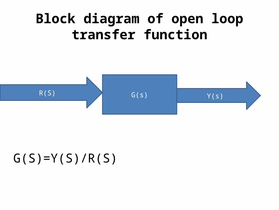
Block diagram of open loop transfer function
R(S) G(s) Y(s)
G(S)=Y(S)/R(S)

Advantages of transfer function
• Its provide the gain of the system.• Integral and differential equation are
converted to algebraic equation. • The transfer function is dependent on the
parameters of the system and independent of the system.
• If transfer function G(s) is known than any output for any given input , can be known.

Disadvantages
• Transfer function can be calculated only for linear and time invariant system.
• Consider only when initial condition are zero.• Its does not give any information about
physical structure of the system.

Poles and Zeros
• Zeros are defined as the root of the polynomial of the numerator of the transfer function.
• Poles are the defined as the root of the polynomial of the denominator of the transfer function.

Generalized transfer function • G(s)=(S-Z1)(S-Z2)----------(S-Zn) (S-P1).(S-P2)---------(S-Pn) Zeros are Z1,Z2,---------Zn and the pole are
P1,P2,------Pn.

Poles of the transfer function
• The value of s which are substitued in the denominator of the transfer function after substituting the value of y the transfer function becomes “infinite “, these values are called poles of the transfer function.
Like P1,P2,------Pn are those value which makes the transfer function infinite when substitute in previous equation.

Zeros of the transfer function
• The value of s which are substituted in the numerator of the transfer function, after substituting the value, the transfer function becomes “Zeros” these values are the called zeros of the transfer function.
Like Z1,Z2,--------Zn are those value which makes the transfer function zero.

Important Point
• When the value of poles and zeros are not repeated , such poles and zeros are called simple poles and zeros . If repeated such poles and zeros are called multiple poles and zeros .
• The order of repeated pole and zeros is equal to the number of times they are repeated.

Poles-Zero Plot
• If we locate all poles and zeros of the transfer function in the s plane (or complex plane ) that diagram is called as the poles-zero plot.
s=σ+jω whereσ= real part and locate on X axis or real axis.jω= imaginary part and locate on Y axis or
imaginary axis.

Poles and Zeros plots
Zeros: roots of N(s)Poles: roots of D(s)Poles must be in the left half plane for the system to be stable.As the poles goes to the closer to the boundary ,the system is the stable.
Stability of Control Systems
• If all the poles of the system lie in left half plane the system is said to be Stable.
• If any of the poles lie in right half plane the system is said to be unstable.
• If pole(s) lie on imaginary axis the system is said to be marginally stable.

• All the poles
s-plane
LHP RHP
j

Examples
10 3,1 if ,)(
CandBABAs
CsG
Then the only pole of the system lie at
Poles =-3
s-plane
LHP RHP
j
X-3

Coding
• P1=[8 56 96];• Q1=[1 4 9 10];• Sys=tf(P1,Q1)• Roots(P1);• Roots(Q1);• pzMAP(sys);

Figure
Coding.2
• Num=[49];• Den=[ 1 4 9 ];• Sys=tf(num,den);• load ltiexamples• ltiview

Graph

Coding
• Num=[49 89 96];• Den=[1 4 9];• Sys=tf[Num,Den];• Load ltiexamples• ltiview

Graph