Flow velocity estimation by complex ambiguity free joint Spectral and Time domain Optical Coherence...

Flow velocity estimation by complex ambiguity

free joint Spectral and Time domain Optical

Coherence Tomography

Maciej Szkulmowski, Ireneusz Grulkowski, Daniel Szlag, Anna Szkulmowska, Andrzej

Kowalczyk, and Maciej Wojtkowski*

Institute of Physics, Nicolaus Copernicus University, ul. Grudziądzka 5/7, PL-87-100 Toruń, Poland *[email protected]

Abstract: We show that recently introduced joint Spectral and Time

domain Optical Coherence Tomography (STdOCT) can be used for

simultaneous complex ambiguity removal and functional Spectral OCT

images. This permits to take advantage of higher sensitivity achievable near

the zero-path delay. The technique can be used with all Spectral OCT

systems that are equipped with an optical delay line (ODL) and provide

oversampled scanning patterns. High sensitivity provided by STdOCT

allows this technique to be used in Spectral OCT setups with acquisition

speed of 100 000 lines/s. We show that different imaging ranges and

velocity ranges can be achieved by switching on/off the ODL and a small

modification in the processing algorithm. Additionally, the relatively small

computational burden of the technique allows for fast computations in the

range of less than 5 minutes for 3D data set. We present application of

proposed technique to full-range two- and three-dimensional imaging.

Morphological and Doppler tomograms of human retina in-vivo are shown.

Finally, we identify and discuss artifacts of the technique.

©2009 Optical Society of America

OCIS codes: (170.4500) Optical coherence tomography; (170.3880) Medical and biological

imaging; (170.4470) Ophthalmology; (280.2490) Flow diagnostics.

References and links

1. D. Huang, E. A. Swanson, C. P. Lin, J. S. Schuman, W. G. Stinson, W. Chang, M. R. Hee, T. Flotte, K. Gregory,

C. A. Puliafito, and J. G. Fujimoto, “Optical coherence tomography,” Science 254(5035), 1178–1181 (1991).

2. A. F. Fercher, C. K. Hitzenberger, G. Kamp, and S. Y. Elzaiat, “Measurement of Intraocular Distances by

Backscattering Spectral Interferometry,” Opt. Commun. 117(1–2), 43–48 (1995).

3. G. Hausler, and M. W. Lindner, ““Coherence radar” and “spectral radar”-new tools for dermatological

diagnosis,” J. Biomed. Opt. 3(1), 21–31 (1998).

4. M. A. Choma, M. V. Sarunic, C. H. Yang, and J. A. Izatt, “Sensitivity advantage of swept source and Fourier

domain optical coherence tomography,” Opt. Express 11(18), 2183–2189 (2003).

5. R. Leitgeb, C. K. Hitzenberger, and A. F. Fercher, “Performance of fourier domain vs. time domain optical

coherence tomography,” Opt. Express 11(8), 889–894 (2003).

6. M. Wojtkowski, V. J. Srinivasan, T. H. Ko, J. G. Fujimoto, A. Kowalczyk, and J. S. Duker, “Ultrahigh-

resolution, high-speed, Fourier domain optical coherence tomography and methods for dispersion

compensation,” Opt. Express 12(11), 2404–2422 (2004).

7. R. Leitgeb, M. Wojtkowski, A. Kowalczyk, C. K. Hitzenberger, M. Sticker, and A. F. Fercher, “Spectral

measurement of absorption by spectroscopic frequency-domain optical coherence tomography,” Opt. Lett.

25(11), 820–822 (2000).

8. R. A. Leitgeb, C. K. Hitzenberger, A. F. Fercher, and T. Bajraszewski, “Phase-shifting algorithm to achieve high-

speed long-depth-range probing by frequency-domain optical coherence tomography,” Opt. Lett. 28(22), 2201–

2203 (2003).

9. B. Vakoc, S. Yun, J. de Boer, G. Tearney, and B. Bouma, “Phase-resolved optical frequency domain imaging,”

Opt. Express 13(14), 5483–5493 (2005).

10. S. Makita, Y. Hong, M. Yamanari, T. Yatagai, and Y. Yasuno, “Optical coherence angiography,” Opt. Express

14(17), 7821–7840 (2006).

(C) 2009 OSA 3 August 2009 / Vol. 17, No. 16 / OPTICS EXPRESS 14281#111799 - $15.00 USD Received 22 May 2009; revised 22 Jul 2009; accepted 24 Jul 2009; published 31 Jul 2009

11. A. Szkulmowska, M. Szkulmowski, A. Kowalczyk, and M. Wojtkowski, “Phase-resolved Doppler optical

coherence tomography - limitations and improvements,” Opt. Lett. 33(13), 1425–1427 (2008).

12. R. K. Wang, S. L. Jacques, Z. Ma, S. Hurst, S. R. Hanson, and A. Gruber, “Three dimensional optical

angiography,” Opt. Express 15(7), 4083–4097 (2007).

13. L. An, and R. K. Wang, “In vivo volumetric imaging of vascular perfusion within human retina and choroids with

optical micro-angiography,” Opt. Express 16(15), 11438–11452 (2008).

14. Y. K. Tao, A. M. Davis, and J. A. Izatt, “Single-pass volumetric bidirectional blood flow imaging spectral

domain optical coherence tomography using a modified Hilbert transform,” Opt. Express 16(16), 12350–12361

(2008).

15. Y. Yasuno, S. Makita, T. Endo, G. Aoki, M. Itoh, and T. Yatagai, “Simultaneous B-M-mode scanning method for

real-time full-range Fourier domain optical coherence tomography,” Appl. Opt. 45(8), 1861–1865 (2006).

16. Y. K. Tao, K. M. Kennedy, and J. A. Izatt, “Velocity-resolved 3D retinal microvessel imaging using single-pass

flow imaging spectral domain optical coherence tomography,” Opt. Express 17(5), 4177–4188 (2009).

17. R. K. Wang, and L. An, “Doppler optical micro-angiography for volumetric imaging of vascular perfusion in

vivo,” Opt. Express 17(11), 8926–8940 (2009).

18. M. Szkulmowski, A. Szkulmowska, T. Bajraszewski, A. Kowalczyk, and M. Wojtkowski, “Flow velocity

estimation using joint Spectral and Time domain Optical Coherence Tomography,” Opt. Express 16(9), 6008–

6025 (2008).

19. A. Szkulmowska, M. Szkulmowski, D. Szlag, A. Kowalczyk, and M. Wojtkowski, “Three-dimensional

quantitative imaging of retinal and choroidal blood flow velocity using joint Spectral and Time domain Optical

Coherence Tomography,” Opt. Express 17(13), 10584–10598 (2009).

20. M. Wojtkowski, A. Kowalczyk, R. Leitgeb, and A. F. Fercher, “Full range complex spectral optical coherence

tomography technique in eye imaging,” Opt. Lett. 27(16), 1415–1417 (2002).

21. M. A. Choma, C. H. Yang, and J. A. Izatt, “Instantaneous quadrature low-coherence interferometry with 3 x 3

fiber-optic couplers,” Opt. Lett. 28(22), 2162–2164 (2003).

22. P. Targowski, W. Gorczynska, M. Szkulmowski, M. Wojtkowski, and A. Kowalczyk, “Improved complex

spectral domain OCT for in vivo eye imaging,” Opt. Commun. 249(1–3), 357–362 (2005).

23. M. V. Sarunic, B. E. Applegate, and J. A. Izatt, “Spectral domain second-harmonic optical coherence

tomography,” Opt. Lett. 30(18), 2391–2393 (2005).

24. R. K. K. Wang, “In vivo full range complex Fourier domain optical coherence tomography,” Appl. Phys. Lett.

90(5), 054103 (2007).

25. Y. K. Tao, M. Zhao, and J. A. Izatt, “High-speed complex conjugate resolved retinal spectral domain optical

coherence tomography using sinusoidal phase modulation,” Opt. Lett. 32(20), 2918–2920 (2007).

26. E. Götzinger, M. Pircher, and C. K. Hitzenberger, “High speed spectral domain polarization sensitive optical

coherence tomography of the human retina,” Opt. Express 13(25), 10217–10229 (2005).

27. Y. Yasuno, S. Makita, T. Endo, G. Aoki, H. Sumimura, M. Itoh, and T. Yatagai, “One-shot-phase-shifting

Fourier domain optical coherence tomography by reference wavefront tilting,” Opt. Express 12(25), 6184–6191

(2004).

28. S. Makita, T. Fabritius, and Y. Yasuno, “Full-range, high-speed, high-resolution 1 microm spectral-domain

optical coherence tomography using BM-scan for volumetric imaging of the human posterior eye,” Opt. Express

16(12), 8406–8420 (2008).

29. M. Szkulmowski, A. Wojtkowski, T. Bajraszewski, I. Gorczynska, P. Targowski, W. Wasilewski, A. Kowalczyk,

and C. Radzewicz, “Quality improvement for high resolution in vivo images by spectral domain optical

coherence tomography with supercontinuum source,” Opt. Commun. 246(4–6), 569–578 (2005).

30. I. Grulkowski, M. Gora, M. Szkulmowski, I. Gorczynska, D. Szlag, S. Marcos, A. Kowalczyk, and M.

Wojtkowski, “Anterior segment imaging with Spectral OCT system using a high-speed CMOS camera,” Opt.

Express 17(6), 4842–4858 (2009).

31. S. H. Yun, G. J. Tearney, J. F. de Boer, and B. E. Bouma, “Motion artifacts in optical coherence tomography with

frequency-domain ranging,” Opt. Express 12(13), 2977–2998 (2004).

32. A. H. Bachmann, M. L. Villiger, C. Blatter, T. Lasser, and R. A. Leitgeb, “Resonant Doppler flow imaging and

optical vivisection of retinal blood vessels,” Opt. Express 15(2), 408–422 (2007).

33. A. G. Podoleanu, G. M. Dobre, and D. A. Jackson, “En-face coherence imaging using galvanometer scanner

modulation,” Opt. Lett. 23(3), 147–149 (1998).

34. R. A. Leitgeb, R. Michaely, T. Lasser, and S. C. Sekhar, “Complex ambiguity-free Fourier domain optical

coherence tomography through transverse scanning,” Opt. Lett. 32(23), 3453–3455 (2007).

35. L. An, and R. K. Wang, “Use of a scanner to modulate spatial interferograms for in vivo full-range Fourier-

domain optical coherence tomography,” Opt. Lett. 32(23), 3423–3425 (2007).

36. B. Baumann, M. Pircher, E. Götzinger, and C. K. Hitzenberger, “Full range complex spectral domain optical

coherence tomography without additional phase shifters,” Opt. Express 15(20), 13375–13387 (2007).

37. B. H. Park, M. C. Pierce, B. Cense, S. H. Yun, M. Mujat, G. Tearney, B. Bouma, and J. de Boer, “Real-time

fiber-based multi-functional spectral-domain optical coherence tomography at 1.3 microm,” Opt. Express 13(11),

3931–3944 (2005).


1. Introduction

Optical Coherence Tomography (OCT) [1] is one of the most rapidly developing techniques

for imaging internal structure of semitransparent objects with micrometer resolution. OCT

with Fourier domain detection (FdOCT) [2,3] enables rapid data acquisition with high

imaging speed and sensitivity [4–6]. A spectrometer-based FdOCT system called Spectral

OCT (SOCT) provides a direct access to spectral fringe signal, which makes it possible to

analyze the evolution of amplitude and phase of light propagating inside the sample under

investigation [7]. This makes SOCT very well suited for estimation of flow velocity of

physiological fluids. Lately, flow velocity estimation attracts investigators’ attention. Reliable

and efficient techniques for qualitative and quantitative estimation of the flow are explored.

The most straightforward way of quantitative velocity estimation is to compare the evolution

of phase in several SOCT spectral interferometric signals acquired consecutively in time. A

measurement technique related to this idea is called phase-resolved Doppler Optical

Coherence Tomography [8–11]. In this technique, the frequency of the spectral fringes

encodes the axial position of the scattering particle, while the phase change is proportional to

its velocity. In this approach the quantitative information of the velocity is well localized

spatially as only few spectra are processed at once. More recently, several techniques have

appeared which compute the Doppler frequency along the time axis directly by means of

Fourier transformation instead of using the phase shift analysis [12–14]. Most of these

techniques evolved from the BM-mode scanning method originally proposed by Yasuno et al.

[15]. BM-mode OCT has been initially designed for complex ambiguity removal, where the

Fourier transformation was applied along the “time”/”lateral position” axis over large amount

of spectra. As a result, the computational burden of the algorithm is minimal but the

quantitative information of flow velocity is lost and the low velocity flows are invisible.

Therefore, the algorithms derivative to BM-mode focus mainly on segmentation of the vessel

network, which is achieved by filtering out all static structural elements instead of measuring

and calculating spatially distributed velocity values. Quantitative analysis of flow velocities is

rendered very difficult in these approaches because the filtering of the static components of

the sample usually causes a partial removal of information about low velocities. An attempt to

perform a quantitative estimation of flow has been proposed using this technique but it

requires filtering the tomogram several times with different filter settings, what can take few

hours of calculations for a 3D data set [16]. Long calculation time makes the technique

difficult to use in practice. Recently, Wang et al. [17] proposed a technique that combines

phase-resolved approach with filtering in Fourier space. The algorithm is complex and

requires some assumptions about the imaged tissue, but offers an increase in velocity

detection sensitivity.

Another method that exploits Doppler effect to perform velocity measurements is joint

Spectral and Time domain OCT (STdOCT) [18]. This technique uses only amplitudes of

Fourier transformations to estimate the Doppler frequencies and, as compared to phase-

resolved Doppler OCT, offers higher sensitivity and better reliability in quantitative velocity

estimation in the entire velocity range. Additionally, it provides quantitative velocity values

well localized spatially inside the sample and gives good velocity readings for low velocity

values. The latter is caused by the fact that it does not use any thresholds that limit the

velocity range. What is important, the technique does not require the data to be back Fourier

transformed at any stage of the procedure. Consequently, its numerical complexity is only

slightly increased compared to standard phase-resolved OCT imaging with A-scans averaging.

Therefore, the data processing can be performed with the speeds of thousands lines per

second. Recently, we also showed that its high sensitivity makes the technique well suited for

segmentation of the vessel network in 3D data acquired at line-rates of 100 kHz [19].

In order to take advantage of the highest sensitivity achievable in Spectral OCT near the

zero optical path-delay position, the complex conjugate image (“mirror” image) of the sample


should be removed. This would also facilitate imaging of the thick structures such as the

retina in the proximity of the optic nerve head, where large retinal veins and arteries can

appear simultaneously with choroidal vessels. To get rid of the undesired “mirror” images

several techniques such as multi-frame methods [15,20–26] and variants of the BM-mode

technique [15,24,27,28] have been presented to date. Unfortunately, in all of these methods

the phase information associated to the sample and its complex counterpart interfere and

quantitative velocity estimation is no longer possible.

Information encoded in the phase of spectral fringes is used in both velocity estimation

and complex ambiguity removal techniques. These both methods require to use multiple

spectral fringe signals to create one line of either structural or functional image. The spectra

used in the calculations should be acquired at the same lateral position of the scanning beam

in order to obtain well spatially localized phase information. It can be achieved by the lateral

scanning either with a discrete step-like or a continuous ramp driving signal. The latter

approach is more practical due to strong limitations in the settling time of galvanometric

scanners. However, to achieve well defined phase information the continuous lateral scanning

has to be performed along with the high sampling density. Additionally, another

straightforward advantage of using several spectra to create one line of the tomogram is a

sensitivity increase of the structural imaging. This is achieved simply by averaging

backscattered intensities of multiple A-scans.

High sampling density is exploited in a modified joint Spectral and Time domain OCT,

which we demonstrate in this contribution. The presented technique allows for the complex

ambiguity removal simultaneously with quantitative estimation of velocity values in the entire

imaging range. The only required modification in the setup is an optical delay line (ODL) in

the reference arm that allows for introduction of constant velocity offset during data

acquisition. As a result this method is able to work with data acquired with commonly used

high density scanning protocols. One of the main advantages of this technique is that the

calculation time does not exceed a few seconds for a single cross-sectional image. It has to be

noted that doubling the imaging range causes the velocity range to be halved. However, the

flexibility of the technique allows for changing from full imaging range to full velocity range

by simply switching off the ODL.

We believe that the simplicity of the algorithm, ease of implementation in existing SOCT

systems, high sensitivity and numerical efficiency make this new method a practical and

reliable tool for retinal flow analysis.

2. Method

In the first step all spectra have to undergo standard SOCT data preprocessing in order to

transform them from wavelength domain to wavenumber domain (k domain). Next,

uncompensated dispersion is numerically removed and a numerical shaping of the spectral

fringes is introduced [29]. One of the joint Spectral and Time domain OCT technique variants

(described in the following subsections) is applied to the subset of acquired spectra used to

create a single line of structural and velocity tomograms. The procedure is applied several

times to different sets of spectral fringes until all lines of the tomogram are created. The

subsequent subsections describe numerical processing applied to the subset of preprocessed

spectra to create a single line of structural and velocity tomograms.

2.1. Standard STdOCT

The spectral fringe signals selected for calculations can be considered as a two-dimensional

interferogram and expressed in the following way:

( ) ( ) ( ), 2 cos 2 2 .s r s r s s

s s

I k t S k R R R R k v kt

= + + + ∑ ∑ z (1)


The above signal results from interference between light reflected from a stationary

reference mirror (reflectivity coefficient r

R ), and backscattered on several interfaces in the

sample (reflectivity coefficients s

R ). The wavelength dependent spectral envelope is denoted

by ( )S k . The phase of the interferometric signal depends on the positions s

z of the scattering

interfaces as well as on the projections ( )coss s

v V α= of velocity s

V of the scattering particle

in the sample moving in the direction inclined to the probing beam at angle α .

Due to the introduced oversampling, we assume that the lateral distance between

consecutive positions of the probing beam is much smaller than the beam diameter. Because

of this, in Eq. (1) the spectra can be regarded as having been acquired at the same position of

the sample. Therefore, the dependence on the lateral position can be neglected. As a result, the

beat frequency 2s s

v kω = that arises for each wavenumber k along the time axis encodes the

laterally localized velocity of the s-th interface inside the sample. Simultaneously, the

frequency of fringes along the wavenumber axis encodes the axial position of the s-th

interface. It needs to be pointed out that the frequency of fringe pattern carries information

along both spectral and time axes. The observation that the interferogram can be processed in

similar way along both dimensions led to development of the joint Spectral and Time OCT

(STdOCT).

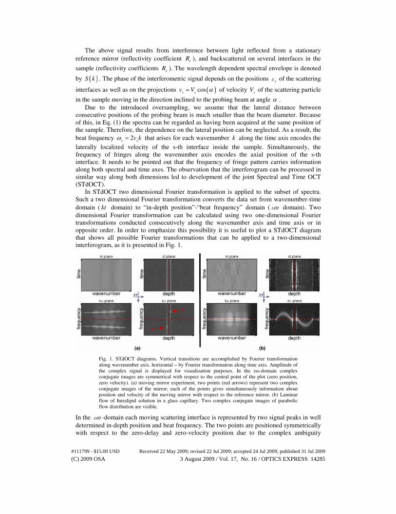
In STdOCT two dimensional Fourier transformation is applied to the subset of spectra.

Such a two dimensional Fourier transformation converts the data set from wavenumber-time

domain ( kt domain) to “in-depth position”-“beat frequency” domain ( ωz domain). Two

dimensional Fourier transformation can be calculated using two one-dimensional Fourier

transformations conducted consecutively along the wavenumber axis and time axis or in

opposite order. In order to emphasize this possibility it is useful to plot a STdOCT diagram

that shows all possible Fourier transformations that can be applied to a two-dimensional

interferogram, as it is presented in Fig. 1.

Fig. 1. STdOCT diagrams. Vertical transitions are accomplished by Fourier transformation

along wavenumber axis, horizontal – by Fourier transformation along time axis. Amplitude of

the complex signal is displayed for visualization purposes. In the zω-domain complex

conjugate images are symmetrical with respect to the central point of the plot (zero position,

zero velocity). (a) moving mirror experiment, two points (red arrows) represent two complex

conjugate images of the mirror; each of the points gives simultaneously information about

position and velocity of the moving mirror with respect to the reference mirror. (b) Laminar

flow of Intralipid solution in a glass capillary. Two complex conjugate images of parabolic

flow distribution are visible.

In the ωz -domain each moving scattering interface is represented by two signal peaks in well

determined in-depth position and beat frequency. The two points are positioned symmetrically

with respect to the zero-delay and zero-velocity position due to the complex ambiguity


problem. This is clearly visible in the case of SOCT signals coming from a moving mirror

Fig. 1(a). The fact that the quantitative distributions of velocity versus depth position can be

directly observed in the ωz -domain is even better visualized in an experiment with Intralipid

solution flowing in a capillary, Fig. 1(b). Here we can observe the parabolic flow velocity

distribution indicating a laminar flow.

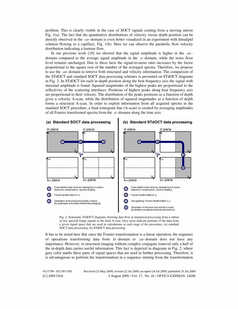
In our previous work [18] we showed that the signal amplitude is higher in the ωz -

domain compared to the average signal amplitude in the tz -domain, while the noise floor

level remains unchanged. Due to these facts the signal-to-noise ratio increases by the factor

proportional to the square root of the number of the averaged spectra. Therefore, we propose

to use the ωz -domain to retrieve both structural and velocity information. The comparison of

the STdOCT and standard SOCT data processing schemes is presented on STdOCT diagrams

in Fig. 2. In STdOCT for each in-depth position along the beat frequency axis the signal with

maximal amplitude is found. Squared magnitudes of the highest peaks are proportional to the

reflectivity of the scattering interfaces. Positions of highest peaks along beat frequency axis

are proportional to their velocity. The distribution of the peaks positions as a function of depth

gives a velocity A-scan, while the distribution of squared magnitudes as a function of depth

forms a structural A-scan. In order to exploit information from all acquired spectra in the

standard SOCT procedure, a final tomogram line (A-scan) is created by averaging amplitudes

of all Fourier transformed spectra from the tz -domain along the time axis.

Fig. 2. Schematic STdOCT diagrams showing data flow in numerical processing from a subset

of raw spectral fringe signals to the final A-scan. Grey areas indicate portions of the data from

a given signal space that are used in calculations at each stage of the procedure; (a) standard

SOCT data processing; (b) STdOCT data processing.

It has to be noted here that since the Fourier transformation is a linear operation, the sequence

of operations transforming data from kt -domain to ωz -domain does not have any

importance. However, in structural imaging without complex conjugate removal only a half of

the in-depth data carries useful information. This fact is depicted in diagrams in Fig. 2, where

grey color marks these parts of signal spaces that are used in further processing. Therefore, it

is advantageous to perform the transformation in a sequence starting from the transformation


along wavenumber axis as depicted in Fig. 2(b). This allows the transformation along time

axis to be performed only on one half of the tz -domain thus reducing the calculation burden

by a factor of two.

The possibility of providing information of velocity and morphology simultaneously in

one signal space has to be highlighted as an advantage of the STdOCT over other techniques

using spatial filtering since it is the sole Fourier based technique that does not require the data

to be back transformed at any stage of the procedure. As a result the computation time

required for tomogram reconstruction is only a little bit longer than that for the standard

SOCT method. However, in order to increase the velocity resolution it is required to perform

zero-padding before Fourier transforming the data from tz -domain to the ωz -domain, which

impacts on the computation time.

2.2. Complex ambiguity free STdOCT

In this subsection we show that a small modification to the previously described STdOCT

technique allows for simultaneous velocity estimation and reconstruction of structural A-scans

free from the complex conjugate problem.

Let us now assume that a constant change of optical path difference (OPD) is introduced

between the reference and the sample arm of the interferometer. In the case of the OPD

changes with the velocity ref

v the total time-dependent spectral fringe signal ( ),I k t can be

described by an expression similar to the one shown in Eq. (1):

( ) ( ) ( )( ), 2 cos 2 2 .s r s r s s ref

s s

I k t S k R R R R k v v kt

= + + + + ∑ ∑ z (2)

In the zω-domain the complex conjugate images are positioned on the opposite sides of

both zero-delay line (in case of 0s≠z ) and on opposite sides of zero beat frequency line (in

case of 0s

v ≠ ). It is important to note that by the introduction of the additional velocity

0ref

v ≠ one shifts the image and its complex conjugate counterpart in opposite directions

along the beat frequency axis.

Fig. 3. STdOCT diagrams of Intralipid flow in a glass capillary: (a) without additional velocity;

(b) with additional velocity ref

v (marked by red arrow) introduced in the reference arm of the

interferometer.

If the ODL velocity is large enough, the two images together with all the inner velocity

components are completely separated along the ω axis. This effect is clearly visualized in

Fig. 3(b), which presents data from the same experimental setup as data from Fig. 3(a) but


with additionally introduced velocity ref

v . The conjugate velocity distributions of Intralipid

solution are placed on “positive” and “negative” sides of the beat frequency axis.

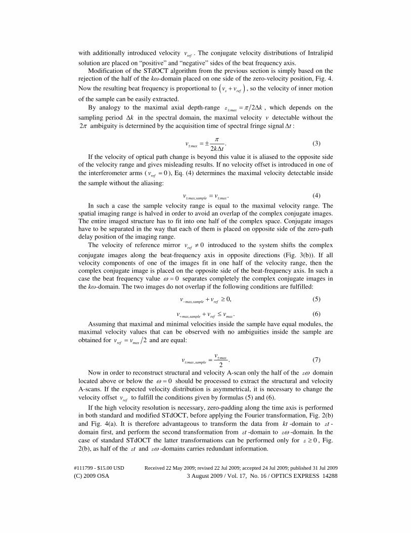
Modification of the STdOCT algorithm from the previous section is simply based on the

rejection of the half of the kω-domain placed on one side of the zero-velocity position, Fig. 4.

Now the resulting beat frequency is proportional to ( )s refv v+ , so the velocity of inner motion

of the sample can be easily extracted.

By analogy to the maximal axial depth-range 2max

kπ± = ∆z , which depends on the

sampling period k∆ in the spectral domain, the maximal velocity v detectable without the

2π ambiguity is determined by the acquisition time of spectral fringe signal t∆ :

.2

maxv

k t

π± = ±

∆ (3)

If the velocity of optical path change is beyond this value it is aliased to the opposite side

of the velocity range and gives misleading results. If no velocity offset is introduced in one of

the interferometer arms ( 0ref

v = ), Eq. (4) determines the maximal velocity detectable inside

the sample without the aliasing:

.max,sample max

v v± ±= (4)

In such a case the sample velocity range is equal to the maximal velocity range. The

spatial imaging range is halved in order to avoid an overlap of the complex conjugate images.

The entire imaged structure has to fit into one half of the complex space. Conjugate images

have to be separated in the way that each of them is placed on opposite side of the zero-path

delay position of the imaging range.

The velocity of reference mirror 0ref

v ≠ introduced to the system shifts the complex

conjugate images along the beat-frequency axis in opposite directions (Fig. 3(b)). If all

velocity components of one of the images fit in one half of the velocity range, then the

complex conjugate image is placed on the opposite side of the beat-frequency axis. In such a

case the beat frequency value 0ω = separates completely the complex conjugate images in

the kω-domain. The two images do not overlap if the following conditions are fulfilled:

0,max,sample ref

v v− + ≥ (5)

.max,sample ref max

v v v+ + ≤ (6)

Assuming that maximal and minimal velocities inside the sample have equal modules, the

maximal velocity values that can be observed with no ambiguities inside the sample are

obtained for 2ref max

v v= and are equal:

, .2

max

max sample

vv ±± = (7)

Now in order to reconstruct structural and velocity A-scan only the half of the ωz domain

located above or below the 0ω = should be processed to extract the structural and velocity

A-scans. If the expected velocity distribution is asymmetrical, it is necessary to change the

velocity offset ref

v to fulfill the conditions given by formulas (5) and (6).

If the high velocity resolution is necessary, zero-padding along the time axis is performed

in both standard and modified STdOCT, before applying the Fourier transformation, Fig. 2(b)

and Fig. 4(a). It is therefore advantageous to transform the data from kt -domain to tz -

domain first, and perform the second transformation from tz -domain to ωz -domain. In the

case of standard STdOCT the latter transformations can be performed only for 0≥z , Fig.

2(b), as half of the tz and ωz -domains carries redundant information.


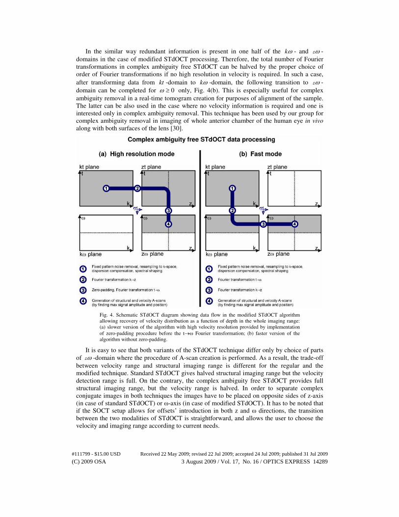
In the similar way redundant information is present in one half of the kω - and ωz -

domains in the case of modified STdOCT processing. Therefore, the total number of Fourier

transformations in complex ambiguity free STdOCT can be halved by the proper choice of

order of Fourier transformations if no high resolution in velocity is required. In such a case,

after transforming data from kt -domain to kω -domain, the following transition to ωz -

domain can be completed for 0ω ≥ only, Fig. 4(b). This is especially useful for complex

ambiguity removal in a real-time tomogram creation for purposes of alignment of the sample.

The latter can be also used in the case where no velocity information is required and one is

interested only in complex ambiguity removal. This technique has been used by our group for

complex ambiguity removal in imaging of whole anterior chamber of the human eye in vivo

along with both surfaces of the lens [30].

Fig. 4. Schematic STdOCT diagram showing data flow in the modified STdOCT algorithm

allowing recovery of velocity distribution as a function of depth in the whole imaging range:

(a) slower version of the algorithm with high velocity resolution provided by implementation

of zero-padding procedure before the t→ω Fourier transformation; (b) faster version of the

algorithm without zero-padding.

It is easy to see that both variants of the STdOCT technique differ only by choice of parts

of ωz -domain where the procedure of A-scan creation is performed. As a result, the trade-off

between velocity range and structural imaging range is different for the regular and the

modified technique. Standard STdOCT gives halved structural imaging range but the velocity

detection range is full. On the contrary, the complex ambiguity free STdOCT provides full

structural imaging range, but the velocity range is halved. In order to separate complex

conjugate images in both techniques the images have to be placed on opposite sides of z-axis

(in case of standard STdOCT) or ω-axis (in case of modified STdOCT). It has to be noted that

if the SOCT setup allows for offsets’ introduction in both z and ω directions, the transition

between the two modalities of STdOCT is straightforward, and allows the user to choose the

velocity and imaging range according to current needs.


In principle there is exactly the same SNR advantage for both the standard and complex

ambiguity free STdOCT techniques. However, in practice introduction of the constant change

of optical path difference (OPD) will cause the fringe wash-out effect, which will decrease the

spectral fringe visibility and the same the sensitivity of our technique [31,32]. We can easily

calculate the magnitude of the fringe wash-out in the case of our optical delay line, since it is

set to the constant velocity value (Eq. (7)) corresponding to the phase shift of λ/8 between

consecutive spectral fringe signals. According to the theoretical analysis presented by

Bachmann et al. [32] the sensitivity drop due to such phase shift is only 1dB.

3. Experimental set-up

3.1. SOCT device

The SOCT system based on fiber-optic Michelson interferometer configuration is shown in

Fig. 5.

Fig. 5. SOCT set-up used in experiments: FC – fiber coupler (splitting ratio 90:10); PC –

polarization controller; L1-L4 – lenses; NDF – neutral density filter; DC – dispersion

compensation; ODL – optical delay line; SM-Z – galvanometer scanner (z-scanning); RM –

reference mirror; SM-XY – galvanometer scanners (xy-scanning); DG – holographic volume

diffraction grating; CMOS – line-scan camera; FG – frame-grabber; COMP – personal

computer; IOC – input-output card.

The light source is a femtosecond Ti:Sapphire laser (Fusion, Femtolasers, ∆λ = 160nm,

central wavelength 810 nm). Light from the laser is launched to an optical single mode fiber

interferometer (AC Photonics Inc., USA) that splits 90% of light energy into the reference

arm and the rest into the object arm. The reference arm is equipped with a neutral density

filter to adjust light intensity as well as with a dispersion controller to minimize the dispersion

mismatch between both arms of the interferometer. Optical delay line (ODL) using

galvanometer-based scanner (Cambridge Technology Inc., USA), collimating achromat lens

(f1 = 19mm) and another achromat lens L2 (f2 = 40mm) is placed in the reference arm.

Detailed description of the ODL is given in the next subsection. The detection arm consists of

a custom designed spectrometer containing an achromatic collimating objective (Schneider

Optics, USA), a volume holographic diffraction grating (1200 lpmm; Wasatch Photonics,

USA) and a f-theta objective (Sill Optics, Germany) imaging the spectral interference fringes

at the 12-bit line scan CMOS camera with 4096 pixels (Sprint, Basler AG, Germany). CMOS

camera was set to acquire 2048 pixels from 4096 available photosensitive elements.

Transversal scanning of the sample is provided by a set of two galvanometer-based optical

scanners (Cambridge Technology Inc., USA). Triggers to all scanners and the camera are

delivered in analog form by an analog input/output card (National Instruments, USA). The

experimental data registration is realized by a framegrabber (National Instruments, USA).


Measured axial resolution in air is equal to 3 µm what corresponds to 2.3 µm in tissue.

Imaging range without the complex ambiguity removal technique equals 1 mm in tissue and is

doubled to 2 mm in case the complex ambiguity removal technique is used. All measurements

were performed with the power of light incident the cornea equal to 750µW at 810 nm.

3.2. Optical delay line

In order to introduce a velocity offset we equipped the reference arm with a simple optical

delay line (ODL) based on galvanometer scanner that deflects the light beam towards the

reference mirror (Fig. 6). The axis of rotation of the scanner is shifted from the point hit by

the light beam, what causes the optical path length of the reference arm to be dependent on the

instantaneous angle of the scanner.

The concept to use the ODL based on a scanner with off-axis illumination has been

exploited recently by several groups [33–36], but they placed it in the sample arm and used

the laterally scanning mirror to introduce the optical path delay. This idea is very elegant but

we deliberately decided not to use it as it couples velocity offset with lateral scanning

parameters. When ODL is placed in the reference arm, it is much easier to introduce an

arbitrary velocity along with arbitrary lateral scanning protocol. It is also possible to switch

the ODL off if necessary. This fact is important because of different trade-offs between

velocity and imaging ranges in standard and complex ambiguity free STdOCT as mentioned

in the method section. Switching off the delay line brings the velocity offset to zero and

enables standard STdOCT to provide full velocity range with limited structural imaging range.

With the aid of this ODL such transition is possible at any moment, for example during

aiming and aligning of the sample.

Fig. 6. (a) Detailed scheme of the optical delay line introduced in the reference arm of the

SOCT set-up used in experiments: L1, L2 – lenses; SM-Z – galvanometric scanner; RM –

reference mirror; f – focal length of the lens L2; For clarity the neutral density filter and

dispersion compensator are removed from the drawing. (b) Parameters used to calculate the

optical path difference: δ – shift between the incoming beam and the axis of rotation of SM-Z;

α – tilt angle of SM-Z; z – optical path distance introduced by scanner tilt. The part of the light

beam marked in red is responsible for optical path difference between the two positions of the

rotating mirror. See text for further details.

When the optical beam is deflected by the mirror attached to the galvanometric scanner SM-Z

in the distance δ from the pivot, the optical path difference ( )δ αz depends on the angle α

between the direction perpendicular to the impinging beam and the surface of the scanner:

( ) ( )tan .δ α δ α=z (8)

Taylor expansion of the above expression around an initial angle 0

α yields:


( ) ( )( )

( ) ( ) ( )2

0 0 0 02

0

1 1tan sin 2 .

2cosδ α δ α α α α α α

α

≅ + ⋅ − + ⋅ − +

…z (9)

In this expression the quadratic term can be omitted, since it is usually much smaller than the

linear part. This allows for calculation of the velocity introduced by the scanner rotating with

angular frequency SM-Z

d dtω α= :

( )( ) SM-Z2

0

22 .

cosref

dv

dtδ

δα ω

α= = ⋅z (10)

The factor 2 is a consequence of the fact that the light travels the path ( )δ αz twice.

In the configuration used in our experiments, the angle 0

45α = ° , therefore Eq. (10)

simplifies to:

SM-Z

4 .ref

v δ ω= ⋅ (11)

4. Results and discussion

4.1. Extinction ratio and scanning protocols for complex ambiguity free STdOCT

In order to measure the extinction ratio of the complex conjugate removal in STdOCT

method, we performed experiment with one static mirror and one moving mirror in the

interferometer arms. Measured ratio of the complex conjugate remaining signals to the peak

corresponding to the mirror position was −22dB and −30dB for 16 and 32 spectral fringes

used for STdOCT analysis.

The SOCT setup operates in two main modes. The preview mode displays two structural

tomograms (each of 420 A-scans created from 2172 spectra) acquired perpendicularly to each

other in horizontal and vertical directions. These two images are used for alignment of the

head of the device (probing beam) with respect to the sample. Fast mode of complex

ambiguity free STdOCT, Fig. 4(b), allows for real-time display of images at 5 frames/sec.

The imaging mode uses high velocity resolution mode of complex ambiguity free

STdOCT, Fig. 4(a), and provides structural and velocity tomograms in two or three

dimensions. As mentioned in previous sections in order to be able to perform quantitative

velocity estimation lateral shift between the positions of the scanning beam has to be smaller

than the beam diameter, which is assumed to be 20 µm at the retina. Spectra are acquired at

100 000 lines/s with the integration time of 8.7 µs. As a result, the maximal velocity range

maxv is equal to 20.2 mm/s for standard imaging and 10.1 mm/s for complex ambiguity free

imaging. Examples of scanning protocols that fulfill this condition are presented in Table 1. It

can be seen that in all cases the lateral oversampling factor [37] which is the ratio of the

sampling density to the beam width is not larger 0.2.

Table 1. Scanning protocols used in experiments with complex ambiguity free STdOCT.

Protocol No.

spectra

Lateral

dimensions

Sampling density

[µm/scan]

Sampling density

/beam width

Measurement

time [s]

2D_1 5430x1 4mm x 0mm 0.74 0.037 0.054

2D_2 8688x1 5mm x 0mm 0.58 0.029 0.087

3D_1 2172x100 5mm x 5mm 2.30 0.115 2.172

The signal driving the galvanometer scanner in the ODL is triangular. The angular

frequency of the scanner is set to introduce reference velocity 2ref max

v v= , which provides

maximal velocity range, according to Eq. (7). The amplitude of the scanner driving signal


remains constant. Exactly 543 spectra acquisitions are performed along each monotonic ramp

of the signal. The triangular signal is synchronized with the beginning of every B-scan. In all

cases one final A-scan is constructed from 16 spectral fringe signals. To create B-scans or

velocity maps with a reasonable quality we divided our initial 543 spectral fringes into 105

partially redundant sets of 16 spectral fringes (105 ( )543 16 5= − ). Separation between

each set of 16 fringes is chosen to be 5, only to optimize the calculation time. This procedure

introduces some kind of smoothing or interpolation into the velocity maps. Zero-padding (z-

axis) up to 128 data points is performed before applying Fourier transformation, Fig. 2(b) and

Fig. 4(a).

The calculations are performed with our software written in C and run on a personal

portable computer (HP Compaq 8510w). The average computation time in all the above

examples (in high velocity resolution mode) is about 1000 final tomogram lines per second.

Total computation time depends on the protocol and is equal 6.7 seconds for the 2D_1

protocol, 9.5 seconds for 2D_2 protocol and 286 seconds (approx. 5 minutes) for 3D_1

protocol.

4.2. Complex ambiguity free STdOCT

In order to show the capability of the complex ambiguity free STdOCT technique to provide

mirror free velocity and structural tomograms, we performed experiments of in-vitro flows in

glass capillaries as well as in retinal vessels in-vivo.

Fig. 7. STdOCT measurement of two glass capillaries with Intralipid solution. (a) structural

cross-sectional image obtained using standard STdOCT processing; (b) velocity map obtained

using phase-resolved OCT max

20.2 mm/sv = ; (c) structural cross-sectional image obtained

using complex ambiguity free STdOCT; (d) velocity map obtained using complex ambiguity

free STdOCT max

10.1mm/sv = .

In the first experiment water solution of Intralipid flowing inside two glass capillaries of

700 µm diameter was imaged. Laminar flow of the fluid was assured by a HPLC (High

performance liquid chromatography) pump (Selko Industries, Poland). Scanning protocol

2D_1 described in Table 1 was utilized. Fig. 7(a) shows a cross-sectional image obtained by

application of standard STdOCT algorithm with immobilized ODL. Fig. 7(b) depicts velocity

tomogram obtained with aid of standard phase-resolved [11]. Two complex conjugate (mirror)


images are visible in both tomograms. Figs. 7(c) and 7(d) present structural and velocity

tomograms free from one of the mirror images. The data were obtained with the ODL turned

on. In the following experiments data were acquired from human retina in-vivo using scanning

protocol 2D_2, Table 1. Results are shown in Fig. 8. Sixteen spectra are used to create a single

A-scan of the velocity map and complex ambiguity free cross-sectional image from the lateral

range of 5 mm. As a result, the effective lateral resolution drops approximately by 50%, to 30

µm. The complex conjugate image is suppressed in both structural and velocity images.

Fig. 8. High density cross-sectional image of human optic disk in-vivo obtained using complex

ambiguity free STdOCT: (a) structural tomogram; (b) velocity tomogram

max10.1mm/sv = .

The scanning protocol 3D_1 was used to create 3D data set (Table 1). Because we are

analyzing 5x5mm region the effective lateral resolution is 60 µm. Moreover, one can notice

that the complex conjugate images are almost removed. The remaining parts of the vessels

marked by red arrows in Fig. 9(b) and Fig. 9(d) are discussed in the next subsection.


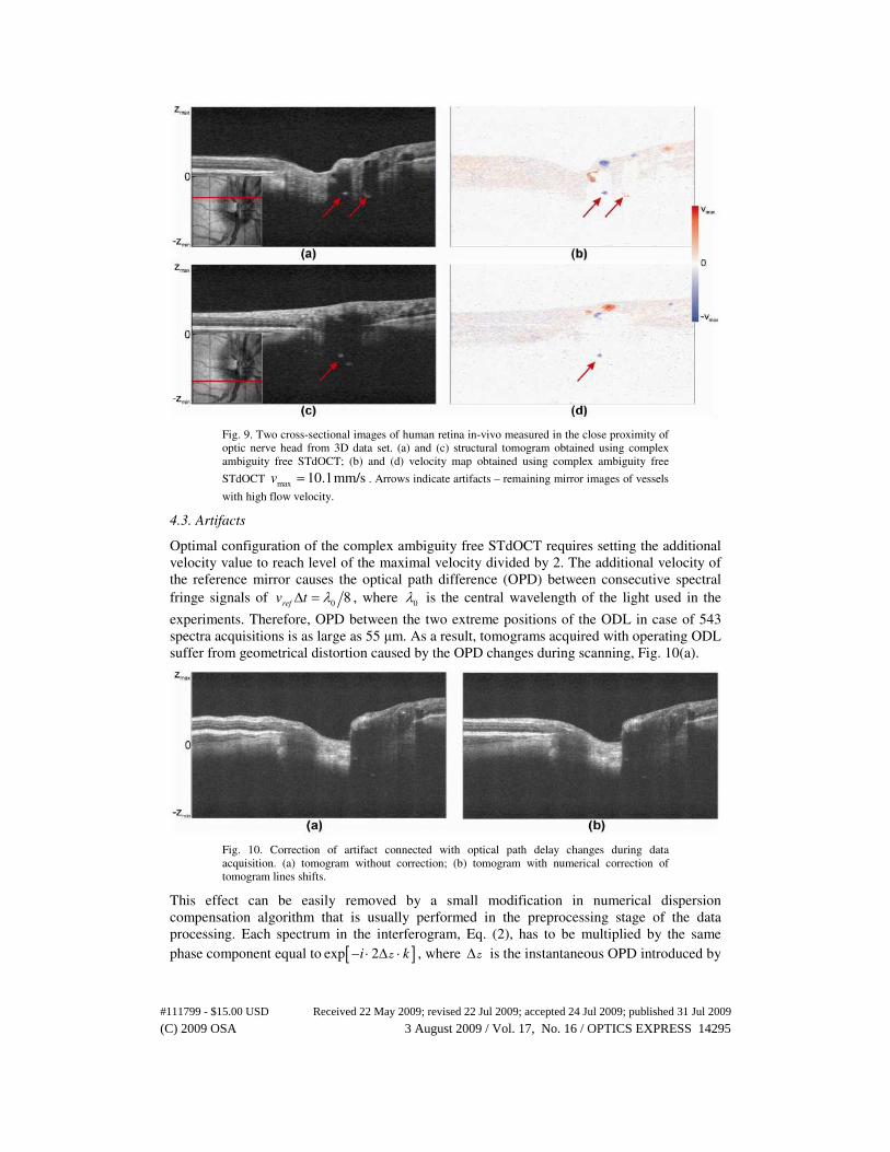
Fig. 9. Two cross-sectional images of human retina in-vivo measured in the close proximity of

optic nerve head from 3D data set. (a) and (c) structural tomogram obtained using complex

ambiguity free STdOCT; (b) and (d) velocity map obtained using complex ambiguity free

STdOCT max

10.1mm/sv = . Arrows indicate artifacts – remaining mirror images of vessels

with high flow velocity.

4.3. Artifacts

Optimal configuration of the complex ambiguity free STdOCT requires setting the additional

velocity value to reach level of the maximal velocity divided by 2. The additional velocity of

the reference mirror causes the optical path difference (OPD) between consecutive spectral

fringe signals of 0

8ref

v t λ∆ = , where 0λ is the central wavelength of the light used in the

experiments. Therefore, OPD between the two extreme positions of the ODL in case of 543

spectra acquisitions is as large as 55 µm. As a result, tomograms acquired with operating ODL

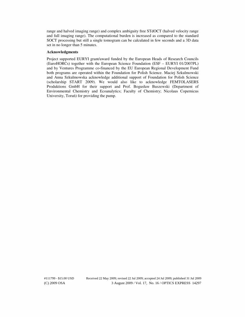
suffer from geometrical distortion caused by the OPD changes during scanning, Fig. 10(a).

Fig. 10. Correction of artifact connected with optical path delay changes during data

acquisition. (a) tomogram without correction; (b) tomogram with numerical correction of

tomogram lines shifts.

This effect can be easily removed by a small modification in numerical dispersion

compensation algorithm that is usually performed in the preprocessing stage of the data

processing. Each spectrum in the interferogram, Eq. (2), has to be multiplied by the same

phase component equal to [ ]exp 2i k− ⋅ ∆ ⋅z , where ∆z is the instantaneous OPD introduced by


the ODL at the moment of acquisition of the central spectrum from the interferogram. Since

the phase element is constant for each A-scan of the tomogram, it can be calculated once and

tabularized. Therefore, it can be incorporated in numerical dispersion compensation algorithm

at no additional computational cost. The result of the procedure is depicted in Fig. 10(b),

where the geometrical distortion is no longer present. This procedure has been applied to all

tomograms presented in this paper.

The second artifact appears when the velocity of the inner motion of the sample does not

fulfill conditions formulated by Eq. (5) and Eq. (6) and it is larger than the velocity limits. In

such a case the parts of the complex conjugate image are visible in the resulting image. This

effect is clearly visible in Fig. 11 as well as in Figs. 9(b) and 9(d). The signal in ωz -domain

reveals the parabolic distribution of flow inside the vessel wrapped to the opposite side of the

velocity range and thus entering on the opposite side of beat frequency domain, see dotted

arrow in Fig. 11(c). Similar artifact has already been reported by Makita et al. [28] and is also

the basis of the vessel segmentation technique proposed by Wang et al. [12].

The solution to this problem is to increase the available velocity range, what can be done

by increasing the line-rate of the acquisition system. Obvious possibility is just to switch off

the optical delay line and perform standard STdOCT imaging to double the velocity range but

the cost to be paid in such a case is the limited imaging range.

Fig. 11. Artifacts appearing when actual flow velocity exceeds velocity range. (a) Structural

tomogram with vessel from the complex conjugate image visible (arrows); (b) velocity

tomogram of (a), max

10.1mm/sv = ; (c) signal in ωz -plane corresponding to the

tomogram line (dotted line), parabolic velocity distribution cross the velocity range limit.

5. Conclusions

We showed that the joint Spectral and Time domain OCT is a straightforward and

computationally efficient data processing scheme that can take advantage of the ultra-high

speed OCT imaging of more than 100 000 lines/s. It can be used with any densely sampled

scanning protocols and can be incorporated in standard Spectral OCT setups. Simple

modification to the algorithm combined with an optical delay line in the reference arm can

provide structural and functional complex ambiguity free cross-sectional images. High

flexibility of the algorithm allows for rapid changes between standard STdOCT (full velocity


range and halved imaging range) and complex ambiguity free STdOCT (halved velocity range

and full imaging range). The computational burden is increased as compared to the standard

SOCT processing but still a single tomogram can be calculated in few seconds and a 3D data

set in no longer than 5 minutes.

Acknowledgments

Project supported EURYI grant/award funded by the European Heads of Research Councils

(EuroHORCs) together with the European Science Foundation (ESF – EURYI 01/2007PL)

and by Ventures Programme co-financed by the EU European Regional Development Fund

both programs are operated within the Foundation for Polish Science. Maciej Szkulmowski

and Anna Szkulmowska acknowledge additional support of Foundation for Polish Science

(scholarship START 2009). We would also like to acknowledge FEMTOLASERS

Produktions GmbH for their support and Prof. Bogusław Buszewski (Department of

Environmental Chemistry and Ecoanalytics; Faculty of Chemistry; Nicolaus Copernicus

University, Toruń) for providing the pump.


Flow velocity estimation by complex ambiguity free joint Spectral and Time domain Optical Coherence...

Documents

Transcript of Flow velocity estimation by complex ambiguity free joint Spectral and Time domain Optical Coherence...