Contents poznanie czasowo-przestrzennej ewolucji procesu ichemisji oraz roli jaka˛odgrywaja˛ w...

Contents

Abstract (in polish) 5

Abstract (in english) 10

Acknowledgments 14

Introduction 16

1 Some base concepts of Heavy-Ion Collision Physics 18

1.1 The QCD phase diagram and the QGP . . . . . . . . . . . . . . . . . . . . . .. 18

1.2 Relativistic heavy-ion collisions . . . . . . . . . . . . . . . . . .. . . . . . . . 22

2 Properties of bulk matter - review of experimental results 26

2.1 Soft processes . . . . . . . . . . . . . . . . . . . . . . . . . . . . . . . . . . .. 26

2.1.1 Inclusive and semi-inclusive particle production - thermal equilibrium

signatures . . . . . . . . . . . . . . . . . . . . . . . . . . . . . . . . . . 26

2.1.2 Chemical equilibrium signatures . . . . . . . . . . . . . . . . . .. . . . 28

2.1.3 The (pseudo-)rapidity density . . . . . . . . . . . . . . . . . . .. . . . 30

2.1.4 “Net” baryon density . . . . . . . . . . . . . . . . . . . . . . . . . . . .31

2.1.5 Strangeness Recombination . . . . . . . . . . . . . . . . . . . . . . .. 32

2.1.6 Flow . . . . . . . . . . . . . . . . . . . . . . . . . . . . . . . . . . . . 35

2.2 Hard processes . . . . . . . . . . . . . . . . . . . . . . . . . . . . . . . . . . .37

1

2.2.1 Jet quenching . . . . . . . . . . . . . . . . . . . . . . . . . . . . . . . . 40

2.2.2 Direct photons . . . . . . . . . . . . . . . . . . . . . . . . . . . . . . . 43

2.2.3 Production of heavy flavors . . . . . . . . . . . . . . . . . . . . . . .. 45

2.3 Perfect Liquid . . . . . . . . . . . . . . . . . . . . . . . . . . . . . . . . . . .. 47

3 Heavy-ion Collision Models 49

3.1 UrQMD . . . . . . . . . . . . . . . . . . . . . . . . . . . . . . . . . . . . . . . 50

3.2 EPOS . . . . . . . . . . . . . . . . . . . . . . . . . . . . . . . . . . . . . . . . 53

3.3 Hydrodynamics . . . . . . . . . . . . . . . . . . . . . . . . . . . . . . . . . . .55

4 Two-particle correlations at small relative velocities 57

4.1 Identical non-interacting unpolarized nucleons and pions . . . . . . . . . . . . . 57

4.2 Identical non-interacting polarized nucleons . . . . . . .. . . . . . . . . . . . . 59

4.3 Non-identical interacting nucleons (neutron - proton). . . . . . . . . . . . . . . 59

4.4 Identical interacting particles . . . . . . . . . . . . . . . . . . .. . . . . . . . . 60

4.5 Deuteron formation rate . . . . . . . . . . . . . . . . . . . . . . . . . . .. . . . 60

4.6 The treatment of Coulomb Interaction . . . . . . . . . . . . . . . . .. . . . . . 61

4.7 Combining Strong and Coulomb interaction . . . . . . . . . . . . . .. . . . . . 61

4.8 Parametrization of correlation function of identical pions . . . . . . . . . . . . . 62

4.9 Theoretical predictions forπ − π, p − p andp − p systems . . . . . . . . . . . . 64

4.10 Theoretical basics of non-identical particle correlations . . . . . . . . . . . . . . 67

4.11 The experimental approach . . . . . . . . . . . . . . . . . . . . . . . .. . . . . 70

4.12 An experimental review of identical and non-identicalparticle correlations . . . . 71

4.13 Baryonic systems . . . . . . . . . . . . . . . . . . . . . . . . . . . . . . . . .. 82

5 The STAR experiment 85

5.1 RHIC . . . . . . . . . . . . . . . . . . . . . . . . . . . . . . . . . . . . . . . . 85

5.2 The STAR detector . . . . . . . . . . . . . . . . . . . . . . . . . . . . . . . . .90

5.3 Performance of TPC . . . . . . . . . . . . . . . . . . . . . . . . . . . . . . . .92

2

6 Analysis of two-baryon correlations 98

6.1 Construction of two-particle correlation function . . . .. . . . . . . . . . . . . 98

6.1.1 Track splitting . . . . . . . . . . . . . . . . . . . . . . . . . . . . . . . 100

6.1.2 Track merging . . . . . . . . . . . . . . . . . . . . . . . . . . . . . . . 100

6.1.3 Gamma conversion into electron-positron pairs . . . . .. . . . . . . . . 102

6.2 Corrections . . . . . . . . . . . . . . . . . . . . . . . . . . . . . . . . . . . . . 103

6.2.1 Purity correction . . . . . . . . . . . . . . . . . . . . . . . . . . . . . .103

6.2.2 Resolution smearing correction . . . . . . . . . . . . . . . . . . .. . . 104

6.2.3 Residual correlation correction . . . . . . . . . . . . . . . . . .. . . . . 105

6.3 Residual correlations . . . . . . . . . . . . . . . . . . . . . . . . . . . . .. . . 106

6.3.1 Basics of residual correlation effects . . . . . . . . . . . . .. . . . . . . 106

6.3.2 Combining contributions from several sources . . . . . . .. . . . . . . . 106

6.3.3 Convolution of decay kinematics . . . . . . . . . . . . . . . . . . .. . . 108

6.3.4 Effects on extracted length scales . . . . . . . . . . . . . . . .. . . . . 111

7 Experimental results 112

7.1 Two-proton correlations without residual correlationcorrections . . . . . . . . . 112

7.1.1 Raw data . . . . . . . . . . . . . . . . . . . . . . . . . . . . . . . . . . 112


7.1.3 Purity and resolution smearing corrections . . . . . . . .. . . . . . . . 116

7.1.4 Two-dimensional correlation functions . . . . . . . . . . .. . . . . . . 119

7.2 Two-proton correlations with residual correlation corrections . . . . . . . . . . . 119


7.2.2 The significance of RC correction . . . . . . . . . . . . . . . . . . .. . 120

7.2.3 All corrections applied . . . . . . . . . . . . . . . . . . . . . . . . .. . 120

7.3 An asymmetry between proton and anti-proton emission . .. . . . . . . . . . . 126

7.3.1 Nonidentical particle correlations . . . . . . . . . . . . . .. . . . . . . 126

7.3.2 Spherical Harmonics decomposition . . . . . . . . . . . . . . .. . . . . 130

3

8 Discussion 134

8.1 Importance of residual correlation corrections . . . . . .. . . . . . . . . . . . . 134

8.2 Transverse mass dependencies . . . . . . . . . . . . . . . . . . . . . .. . . . . 135

8.3 Multiplicity dependencies . . . . . . . . . . . . . . . . . . . . . . . .. . . . . . 136

8.4 Comparison with model predictions . . . . . . . . . . . . . . . . . . .. . . . . 138

8.4.1 UrQMD . . . . . . . . . . . . . . . . . . . . . . . . . . . . . . . . . . 138

8.4.2 EPOS . . . . . . . . . . . . . . . . . . . . . . . . . . . . . . . . . . . . 148

8.4.3 UrQMD and EPOS comparison . . . . . . . . . . . . . . . . . . . . . . 158

9 Conclusions 163

Appendix 1- Elementary units, particles and their interactions 168

Appendix 2- Symbol and conventions used 173

Appendix 3- Two-particle separation distributions - comparison of UrQMD and EPOS176

Glossary 180

List of publications 184

List of presentations 188

Bibliography 190

4

Streszczenie pracy

Badania korelacji barion-barion w relatywistycznych zderzeni-

ach jadrowych rejestrowanych w eksperymencie STAR

Projekt jest elementem badan prowadzonych w ramach eksperymentu STAR (Solenoidal Tracker

At RHIC) w Laboratorium BNL (Brookhaven National Laboratory) z wykorzystaniem zderza-

cza ciezkich jonów RHIC (Relativistic Heavy Ion Collider)- (opis kompleksu eksperymental-

nego znajduje sie w Rozdziale 5). Celem eksperymentu STAR jest, ogólnie mówiac, badanie

własnosci materii jadrowej w ekstremalnych stanach gestosci i temperatur. Oczekuje sie,ze

w warunkach uzyskanych wskutek zderzen ciezkich jonów (np. jader złota) przy energii w

srodku masy rzedu 200 GeV/nukleon wytworzony zostanie stan materii jadrowej zwany plazma

kwarkowo-gluonowa (QGP). Wytworzenie QGP nie tylko stwarza mozliwosci badania własnosci

i oddziaływan najdrobniejszych składników struktury materii, ale takze stanowi odtworzenie

jej stanu w pierwszych mikrosekundach istnienia Wszechswiata, zgodnie z hipoteza Wielkiego

Wybuchu.

Rozdział 1 zawiera wprowadzenie do fizyki zderzen ciezkich jonów; pokrótce opisano podstawy

chromodynamiki kwantowej (ang. ’Quantum Chromodynamics’-QCD) oraz przedstawiono

strukture diagramu fazowego.

Wyniki pierwszych lat pomiarów prowadzonych z pomoca czterech eksperymentów w BNL

rzeczywiscie pokazały symptomy wytworzenia stanu materii w którym uwolnione zostały kwarkowe

stopnie swobody. Efekty "gaszenia dzetów"(ang. ’jet quenching’) - obserwowane w azymutal-

nych rozkładach czastek, anomalnych stosunków krotnosci - wyrazane za pomoca tzw. czyn-

nika modyfikacji jadrowej (ang. ’nuclear modification factor’), efekty ruchów kolektywnych -

demonstrowane poprzez wartosci współczynnika opisujacego tzw. przepływy eliptyczne(ang.

’elliptic flow’) i wiele innych, odpowiadaja przejsciu ze stanu materii hadronowej do stanu ma-

terii kwarkowej. Wytworzony stan rózni sie jednak od oczekiwanego stanu nieodziałujacych

5

kwarków; zblizony jest raczej swymi własnosciami do idealnej cieczy.

Rozdział 2 opisuje aktualny status wyników eksperymentalnych i poszukiwan stanu plazmy.

Wyraznie rozrózniono sektor procesów miekkich (w zakresie niskich pedów: p < 2 GeV/c) oraz

twardych (dlap > 2 GeV/c).

Jednym z efektów, który nadal nie znajduje zadawalajacegoobjasnienia, jest rozwój w czasie i

przestrzeni procesu emisji czastek z goracego i ekspandujacego układu powstałego w wyniku

kolizji ciezkich jonów. Efekt ten, znany pod kyptonimem ’RHIC HBT puzzle’, jest fakty-

cznie zbiorem kilku prawidłowosci obserwowanych w wynikach pomiarów korelacyjnych, a nie

dajacych sie ułozyc w spójny obraz z innymi charakterystykami emitowanych cz ˛astek, obser-

wowanymi równoczesnie. (HBT oznacza tu efekt korelacyjny obserwowany dla par czastek

identycznych). Zagadka wyników pomiarów korelacyjnych widoczna jest głównie w korelac-

jach naładowanych pionów. Korelacje tych czastek emitowanych z najwiekszymi krotnosciami,

sa bowiem najlepiej zbadane. W tym kontekscie szczególnego znaczenia nabieraja rezultaty po-

miaru korelacji w układach barionowych.

Rozdział 4 przedstawia metodologie badania korelacji dwuczastkowych oraz przeglad najwazniejszych

wyników eksperymentalnych. Został przedstawiony opis korelacji dla par czastek identycznych

(z wyraznym podziałem na pary fermionowe i bozonowe) oraz nieidentycznych.

Celem przedstawionej pracy jest analiza dwuczastkowych korelacji pedowych w obszarze małych

predkosci wzglednych dla układów dwubarionowych np. proton-proton, antyproton-antyproton,

proton-antyproton oraz w układach dwuczastkowych z udziałem hiperonów. W wyniku tych

badan powstał spójny opis oddziaływan w stanie koncowym (ang. ’Final State Interaction’- FSI)

dla układów złozonych z róznych kombinacji barionów i antybarionów. Wyznaczone zostały

równiez srednie rozmiary obszarów emisji zródeł emitujacych bariony dla dwóch energii zderzenia

(62 oraz200 GeV liczonych na nukleon wsrodku masy układu zderzajacych sie jader) i trzech

centralnosci zderzenia (zderzenia centralne,sredniocentralne oraz peryferyjne liczone w za-

leznosci od procentowego udziału przekroju czynnego na badana reakcje).

Wyniki tej analizy zostały dokładnie omówione w Rozdziale 6 (poswieconym eksperymental-

nym szczegółom analizy par dwubarionowych) oraz w Rozdziale7. Porównanie z otrzymanymi

juz rezultatami badania korelacji w układach mezon-mezon oraz z przewidywaniami dwóch

modeli teoretycznych: UrQMD (Ultra-relativistic QuantumMolecular Model) i EPOS (gdzie

nazwa modelu jest skrótem od: Energy-conserving quantum mechanical multiple-scattering ap-

proach, Partons, Off-shell remnants, Splitting of parton ladders)- zostało umieszczone w Rozdziale

8.

6

Wnioski z pracy zostały przedstawione w Rozdziale 9 i dotyczanastepujacych aspektów:

• W odróznieniu od korelacji identycznych mezonów, a w szczególnosci pionów, gdzie

efekty korelacyjne sa głównie rezultatem statystyki kwantowej (ang. ’Quantum Statistics’-

QS) - korelacje w układach dwubarionowych sa przede wszystkim nastepstwem oddziały-

wan w stanie koncowym (ang. ’Final State Interactions’- FSI), kulombowskich i silnych.

Po drugie, bariony sa czastkami o zasadniczo wiekszych masach niz piony czy kaony,

a emitowane protony sa w duzej czesci, przy energiach akceleratora RHIC, składnikami

zderzajacych sie pocisków nawet w obszarze małych pospiesznosci. Dlatego bardzo wazne

jest poznanie czasowo-przestrzennej ewolucji procesu ichemisji oraz roli jaka odgrywaja

w relacjach pomiedzy ruchami termicznymi i kolektywnymi goracej i ekspandujacej ma-

terii utworzonej w wyniku zderzenia. Porównanie wyników uzyskanych dla par protonów

z analogicznymi wynikami dla par antyprotonów oraz korelacjami w układzie proton-

antyproton, a takze z udziałem hiperonów i zestawienie uzyskanych rezultatów z istnieja-

cymi juz wynikami dla par mezon-mezon, maja zasadnicze znaczeniedla uzyskania kom-

pletnego obrazu koncowego etapu procesu zderzenia relatywistycznych jonów.Własnie

niespójnosc równoczesnego opisu przez modele hydrodynamiczne jednoczastkowych rozkładów

pedowych oraz korelacji dwuczastkowych, stanowi głównyelement ’RHIC HBT puzzle’.

• Po raz pierwszy udało sie uzyskac spójny obraz korelacji barionowych. Po raz pier-

wszy takze mozliwe stało sie badanie korelacji dla układów złozonych z czastek charak-

teryzujacych sie niska krotnoscia produkcji. Przeprowadzone do tej chwili badania w

ramach przedstawianej tu pracy pokazały nie mierzone nigdywczesniej korelacje dla

par antyproton-antyproton. Jako jeden z elementów realizacji tego projektu przeprowad-

zona została takze analiza wpływu tzw. korelacji szczatkowych (ang. ’residual corre-

lations’) na funkcje korelacyjne badanych układów dwunukleonowych. Uwzglednienie

korelacji szczatkowych jest szczególnie istotne w przypadku barionów, poniewaz znaczna

czesc tych, które sa rejestrowane, pochodzi z rozpadów wskutekoddziaływan słabych

i reprezentuje korelacje dla innego układu, w dodatku zdeformowane kinematyka roz-

padu. Dotychczas nie było potrzeby szczegółowej analizy tego typu efektów. Niewielkie

krotnosci barionów produkowanych w zderzeniach przy nizszych energiach, w szczegól-

nosci krotnosci hiperonów, praktycznie uniemozliwiały wykonanie szczegółowej anal-

izy dla układów innych niz dwuprotonowe. Fakt ten sprawiał równiez, ze rola korelacji

szczatkowych nie była zbyt duza. Przy energiach akceleratora RHIC i duzej akceptancji

7

detektora STAR rola tego typu efektów nie moze byc pominieta w analizie. Opracow-

ana w ramach tego projektu technika uwzglednienia korelacji szczatkowych moze zostac

zastosowana równiez i do innych par czastek, gdzie wpływ korelacji szczatkowych na

mierzone korelacje jest istotny.

• Jeszcze jeden rodzaj analizy danych jest szczególnie istotny dla niniejszego projektu. Chodzi

o korelacje czastek nieidentycznych umozliwiajace wyznaczenie czasowo-przestrzennych

asymetrii w emisji dwóch typów czastek np. protonow i antyprotonow lub protonów i

hiperonów. Analiza taka, niemozliwa dla układów czastek identycznych, polega mówiac

najprosciej, na wydzieleniu przypadków, w których czastka okreslonego typu, np. antypro-

ton, emitowana jest z wieksza predkoscia niz druga czastka analizowanej pary. Wydziele-

nie takiego przypadku oraz komplementarnej sytuacji przeciwnej i zastosowanie dedykowanej

temu procedury analizy danych umozliwia uzyskanie informacji, który z dwóch typów

analizowanych czastek został wyemitowany z mniejszych (wczesniejszych), a który z

wiekszych (pózniejszych) obszarów czasowo-przestrzennych. Uzyskane wyniki umozli-

wiły wiec weryfikacje stanu wiedzy uzyskanej klasycznymimetodami interferometrii jadrowej

(HBT) poszerzajac ja o opis zródeł emitujacych bariony.Analiza korelacyjna par proton-

antyproton skonfrontowana z przewidywaniami modeli uwzg˛edniajacych efekty rozprasza-

nia, dowiodła,ze mimo identycznych mas czastek, ichsrednie czasy oraz obszary emisji

nie sa identyczne. Wskutek anihilacji, antyprotony sa emitowanesrednio pózniej oraz/lub

z mniejszych obszarów niz protony.

Ponizej zostaja przedstawione aspekty techniczne i fizyczne opisywanych prac.

Czesc techniczna pracy to:

• Wybór odpowiednich kryteriów selekcji czastek oraz ich par, aby mierzyc korelacje z jak

najmniejszym wpływem efektów detektorowych. W przypadku przeprowadzonej analizy

była to eliminacja nastepujacych efektów:

1. zjawiska przykrywania sie dwóchsladów czastek w detektorze (identyfikacja jednego

sladu czastki zamiast dwóch),

2. zjawiska rozszczepiania siesladu jednej czastki (identyfikacja jednegosladu czastki jako

dwa rózneslady),

3. identyfikacji produktów konwersji kwantów gamma na pary elektron-pozyton, jako pary

proton-antyproton.

8

• Stworzenie oprogramowania umozliwiajacego niezbedne korekcje: na błednie zidenty-

fikowane czastki oraz na zmierzone korelacje szczatkowe.Nalezało takze oszacowac

wpływ skonczonej rozdzielczosci detektora.

Czesc fizyczna pracy składa sie z nastepujacych elementów:

• Przedstawienie wyników analizy w pełni skorygowanych korelacji trzech kombinacji pro-

tonów oraz ich antyczastek. Wszystkie wyniki dla zanalizowanych energii zderzenia oraz

ich centralnosci sa ze soba spójne w zakresie niepewnosci statystycznych i systematy-

cznych. Oprócz rozmiarów zródeł zbadano sekwencje czasowo-przestrzenna emisji par

czastek nieidentycznych.

• Porównanie wyników eksperymentalnych z przewidywaniami modeli uwzgledniajacych

procesy rozproszen wtórnych (UrQMD). Przedstawiona analiza dowiodła,ze wskutek ani-

hilacji antyprotonów z protonami, antyprotony sa emitowane wczesniej oraz/lub z mniejszych

obszarów niz protony.

Zaprezentowane wyniki wskazuja na celowosc kontynuacji badan dla par barionowych w innych

warunkach eksperymentalnych np. w przygotowywanym obecnie eksperymencie ALICE jaki

bedzie realizowany na zderzaczu Large Hadron Collider (LHC)w laboratorium CERN.

9

Abstract

Studies of baryon-baryon correlations in relativistic nuclear col-

lisions registered at the STAR experiment

This work is the part of scientific program of the STAR experiment (Solenoidal Tracker at RHIC)

in BNL (Brookhaven National Laboratory) operated with RHIC (Relativistic Heavy Ion Col-

lider). The main goal of the STAR experiment is to measure theproperties of extremely hot and

dense matter created during heavy-ion collision. STAR complex is described in Chapter 5. It is

expected that as a result of collision of gold nuclei at energy√

sNN = 200 GeV/nucleon a new

form of matter - QGP (Quark Gluon Plasma) will be created. Such new state will enable one to

measure properties of the smallest matter constituents, which is also predicted to have existed

after few micro-second after Big Bang.

Chapter 1 contains the introduction to the heavy-ion collisions; the basics of QCD and phase

diagram is presented.

During first years of operations, the results of four RHIC experiments indicate the formation of

new state of matter. The results ofjet quenching, nuclear modification factor, collective motions

expressed byelliptic flowand many others describe a phase transition from ordinary hadron mat-

ter to quark matter. However, the QGP was expected to reflect properties of ideal gas. Created

matter indicate rather properties of ideal liquid, thus it was calledsQGP(strongly interaction

QGP).

Chapter 2 describes experimental status of QGP research.

Two-particle correlations can also probe matter created during such collisions. The method and

the experimental review is described in Chapter 4. The lengthof homogeneity measured by

femtoscopy methods includes the effects of space-momentumcorrelations. Together with the re-

lations between thermal and collective motions, between chemical and thermal freeze-out, with

the effects of resonance production and secondary rescattering the final image of space-time evo-

10

lution of the system represents a very complex phenomena, whih is difficult to describe quanti-

tatively. A consistent description clearly needs the information coming both from the analysis of

light (pions) and heavy (protons) systems.

A detailed analysis performed already for identical mesons: pions and kaons and the pioneer

work with the pion-kaon correlations have revealed a lot of unexpected effects commonly known

asRHIC HBT puzzle. More information was clearly necessary. This work is a stepforward to

fill this gap and it describes results of correlations for baryonic systems.

The results of this work complement information obtained earlier by theHBT Physics Working

groupof the STAR experiment at BNL.

The following classes of two-particle systems, incident energies and event centralities have been

considered in the frame of this work:

• all combinations of two particle systems consisting of protons and antiprotons: (p − p),

(p − p,p − p),

• two energies of colliding gold nuclei: 200 GeV and 62 GeV per nucleon pair,

• three classes of event centralities, according to the percentage of the total hadronic cross-

section: central (0-10)%, mid-central (10-30)%, peripheral (30-80)%.

The following experimental results (Chapter 7) have been obtained:

• For the first time the analysis of two antiproton correlations has been performed and the

sizes of antiproton emission region in relativistic heavy ion collisions has been estimated.

• For the first time the analysis of two-particle correlationsfor all systems of protons and

antiprotons, simultaneously and in the same experimental conditions, has been performed.

The obtained quantitative results are consistent within the experimental uncertainties.

• For the first time the asymmetry between space-time parameters of proton and antiproton

emission has been analyzed and quantitatively estimated. Asmall asymmetry has been

found, showing that antiprotons are emitted earlier or moreclose to the edge of the emitting

system.

The analysis for all three proton/antiproton systems have been performed in the same way in all

energy/centrality classes; the same event selection criteria have been applied; the same correc-

tions have been introduced and the same approach was used to estimate the influence of residual

11

correlations. Thus the effect of systematic errors was strongly reduced, what is important for the

quantitative comparison and for common analysis of all the results obtained in this work.

Chapter 6 present the analysis chain.

In order to obtain the physics results free of experimental distortions, the methodical analysis has

been performed.

• A set of cuts have been applied for the registered tracks to eliminate the merging effect

which makes that instead of two separate tracks, only one is reconstructed.

• A dedicated analysis of the tracks located very close in the detector space have been per-

formed in order to avoid the splitting effect which causes that instead of one single track,

two track are found.

• The contamination of electron - positron pairs have been removed.

• The effect of finite detector resolution has been taken into account as well.

• A special attention has been put to the effect of residual correlations resulting mainly from

the contamination of the proton/antiproton sample by the particles (also protons or antipro-

tons) coming from the week decays of hyperons. This effect ismuch more pronouced for

protons than for pions. Due to kinematics of lambda-hyperondecay, proton practically

follows the direction of lambda particle in the detector space and cannot be distinguished

experimentally from that coming directly from the interaction point. A detailed procedure

has been developed and the decays of lambda and sigma hyperons have been considered,

including the decay kinematics. The reflection of FSI correlations in the proton/antiproton

hyperon systems, in the studied proton-antiproton correlations have been taken into ac-

count. One should mention here that such analysis of correlations was made for the first

time for the baryonic systems. This can be important for the comparison of the results ob-

tained here with the other results obtained elsewhere, where the residual correlations have

not been taken into account properly.

The following conclusions (Chapter 8 presents discussion) can be drawn:

• The measured vales of proton/anti-proton emission regionsare systematically smaller then

that of pions and kaons with similar transverse momenta. Considering this result on the

base of hydrodynamic approach and taking into account the larger mass of protons with

respect to kaons and pions, one can understand it as an interplay of thermal and collective

12

motion of hot and expanding system. Thus, pairs of lighter particles are on average emitted

from the region of larger dispersion.

• The increase of measured sizes with the event centrality reflects the geometry of the col-

liding systems. This dependence is similar to that for pionsand kaons.

• The values of emission sizes obtained for 200GeV are slightly larger than those for 62GeV.

More statistics is necessary however to make quantitative conclusion.

• The obtained results are in qualitative agreement with the predictions of theoretical models:

UrQMD and EPOS. It is not the case however for the asymmetry results of nonidentical

particle correlations (see below).

• A small, but definitively nonzero, asymmetry shift has been found in the analysis of proton-

antiproton correlations. One should mention here that a relatively large shift was experi-

mentally found earlier for the pion-kaon system. This result is consistent with the hydro-

dynamic description, where the mass differences lead to thespace-time asymmetries. Such

effect cannot be attributed however to the particles with the same masses. The asymmetry

shift is also absent in the results of simulations with the EPOS model but is seen in the

results of UrQMD simulations. The difference between EPOS and UrQMD, important for

the final stage of the interaction dynamics, consistent in the absence of rescattering pro-

cesses in the EPOS model. One can conclude that the annihilation processes at the last

stage of the collision can be responsible for the observed asymmetry. This conclusion is

also consistent with the sign of asymmetry effect, showing that antiprotons are emitted

earlier or more close to the edge of the emitting system than protons.

The analysis performed here is a step forward in the direction of consistent description of the

dynamics of heavy ion collisions, mainly in the part of so called soft processes.

In order to continue such measurements, it is necessary to have more statistics of experimental

data. In a natural way it can be achieved in the next generation experiment ALICE being prepared

now at CERN. Much larger particle multiplicities and the better detection possibilities makes

good perspectives for such measurements.

13

Acknowledgments

First of all, I would like to thank whole STAR Collaboration atthe RHIC community. This re-

search could have never been realized without You. I would like to thank primarily Dr Timothy

Hallman for the possibility of taking part in such excellentproject as the STAR experiment.

Special thanks to my both supervisors: Professor Barbara Erazmus and Professor Jan Pluta, who

inspired me, gave necessary guidance and always supported various ideas. Thanks to You I was

able to live through exciting adventure that I never thoughtcould have happened to me. You

provided necessary encouragements and warm words. I will never forget that You have been

staying with me in the most painful moments as Friends.

I would like to extend my gratitude for support to the whole Heavy-Ion Reaction Group at Faculty

of Physics at Warsaw University of Technology and to SUBATECHlaboratory- for hospitality

during my several stays here.

Valuable discussions with Dr Adam Kisiel and Professor Michael Lisa let me open my mind to

many crucial aspects of the femtoscopic measurements. Theoretical input from numerous dis-

cussions with Professor Klaus Werner and Dr Richard Lednickywas essential. Many thanks to

the all members of GDRE community. This project enables cooperation of many great scientists

from West and Central Europe. Common work during numerous workshops in Nantes have been

teaching me how to exchange experience.

Many, many thanks go for fruitful discussions to the not mentioned yet STAR HBT Group mem-

bers: Dr Sergey Panitkin, Dr Fabrice Retiere, Zbyszek Chajecki, Marcin Zawisza, Maciek Jedy-

nak, Michal Bystersky, Peter Chaloupka, Debasish Das, AnneliBellingeri.

As English is not my native language, I would like to express my deep gratitude to Marek, who

had spent his time and help me to improve English in this thesis.

Special thanks to my Parents. You always support me and neverlet me down. Thank You so

much.

Last, but surely not least I would like to express my deep loveand thanks to my husband Paweł.

You have always been waiting till I come back from various andfrequent trips. I love You for

14

understanding how deep passion Physics is for me, for Your strong and warm arms always when

I need You. You are my Love and the best Friend.

15

Introduction

The ’Big Bang’ is a cosmological model of the Universe, whose primary assertion is that the

Universe has expanded into its current state from a primordial condition of enormous density

and temperature. It has been shown that ’Big Bang’ is consistent with general relativity and with

the cosmological principle, which states that properties of the Universe should be independent

of position or orientation. Observational evidence for the’Big Bang’ includes the analysis of the

spectrum of light from galaxies, which reveals a shift towards longer wavelengths proportional

to each galaxy’s distance in a relationship described by Hubble’s law. Combined with the as-

sumption that observers located anywhere in the Universe would make similar observations (the

Copernican principle), this suggests that space itself is expanding. The ’Big Bang’ is the best

model for the origin and evolution of the universe.

Many scientists have intended to build experimental complexes which would enable reproduction

of conditions that existed just a few moments after the ’Big Bang’. For many years possibilities

of building greater and bigger complexes have been increasing, with maximal reachable energy

rising as well. For such reasons, the theory of high-energy physics must have been formed.

Why high-energy physics? Because particle physics deals withthe study of elementary con-

stituents of matter. ’Elementary’ means here that such particles do not have known structure. In

the beginning of the twentieth century, particle beam energies from accelerators only reached a

few MeV. Experimental techniques made then possible one to consider protons and neutrons as

elementary particles. Nowadays, with advanced experimental complexes, it is possible to mea-

sure even the structure of a single nucleon, and other elementary components as well (quarks and

leptons). Another reason for high energies is that many of the elementary particles are extremely

massive ones, thus (E = mc2) requiring high amounts of energy to be created. The heaviest

elementary particle detected so far is the ’top’ quark (which has to be created as a pair with their

anti-particle), with the mass-energy ofmc2 ≃ 175 GeV - almost 200 times more than that of a

proton.

Nowadays, the biggest operating accelerator is the Relativistic Heavy Ion Collider (see Chapter

16

5), with another one, the Large Hadron Collider at CERN, in the final phase of installation. These

projects enable one to measure the basic structure of elementary matter. Chapter 1 encloses the

basics of heavy-ion collisions. The properties of collision can be deduced by analyzing charac-

teristics of created particles: hadrons, leptons, .. Chapter 2 presents a review of experimental

results. First prerequisites about phase transition from ordinary matter to the partonic phase are

discussed. RHIC results are divided into sectors of soft processes and hard probes. Chapter 2

reviews an experimental status of known properties of bulk matter. In parallel to experimental ob-

servables, theoretical models are presented (Chapter 3), inorder to understand better heavy-ion

collisions. The method to probe the source of emitting particles is two-particle interferome-

try. Chapter 4 contains theoretical description of the correlation technique and an experimental

review of the most exciting results from last few decades as well. As this work is dedicated

to two-baryon femtoscopic measurements, Chapter 4 discusses briefly the most important two-

proton correlation results obtained so far. The RHIC complexand its experiments are presented

in Chapter 5, which is mainly dedicated to the STAR program. Chapters 6, 7 and 8 present results

of proton femtoscopy from the STAR experiment. Chapter 6 describes technical aspects of how

to construct a two - proton, two - anti-proton and proton - anti-proton correlation functions prop-

erly in STAR. Chapter 8 shows experimental results and Chapter 9discusses them comparing

to the model predictions. The aim of this work is to obtain as global and deep view on baryon

correlations as it is possible from experimental and theoretical point of view, in order to learn

more about properties of the emission of protons and anti-protons.

17

Chapter 1

Some base concepts of Heavy-Ion Collision

Physics

Heavy-ion collisions at high energies [1, 2] allow one to study the elementary components of

matter and the interactions between them. Relativistic heavy-ion collisions give also the possi-

bility to study the behavior of nuclear matter under extremely high pressure and temperature. It

is supposed that such conditions were present during first moments after Big Bang [3]. They

can be recreated experimentally in heavy-ion collisions atultra-relativistic energies, using the

colliders, such as Relativistic Heavy Ion Collider (RHIC) (morein Section 4.1) and in the near

future the Large Hadron Collider (LHC).

1.1 The QCD phase diagram and the QGP

During high-energy collisions (for a more detailed description, see Section 1.2) a hot and dense

system of strongly interacting particles is produced. As quarks and gluons are not allowed to

exist separately and thus have to be bind in hadrons at low energy densities, with the increasing

temperature (heating) and/or increasing baryon density (compression), a phase transition may

occur to the state where ordinary hadrons do not exist anymore and where quarks and gluons

become the correct degrees of freedom. This extreme state ofcolor-deconfined matter is called

Quark-Gluon Plasma (QGP) [4, 5, 6, 7, 8, 9, 10, 11]. The theorydescribing strong interactions

confining quarks into hadrons is a quantum field theory called’Quantum Chromodynamics’

(QCD).

18

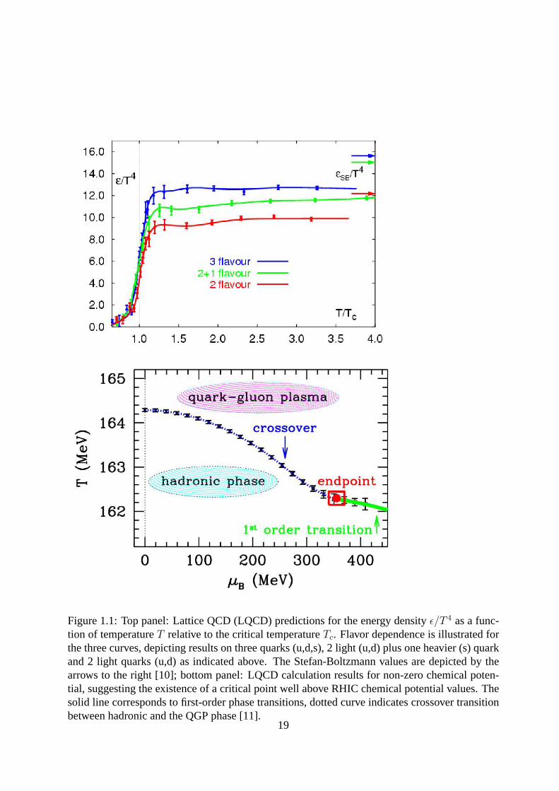
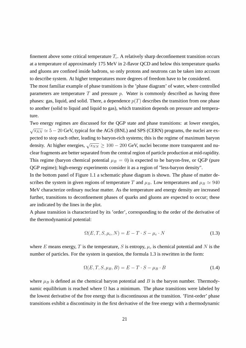
Figure 1.1: Top panel: Lattice QCD (LQCD) predictions for the energy densityǫ/T 4 as a func-tion of temperatureT relative to the critical temperatureTc. Flavor dependence is illustrated forthe three curves, depicting results on three quarks (u,d,s), 2 light (u,d) plus one heavier (s) quarkand 2 light quarks (u,d) as indicated above. The Stefan-Boltzmann values are depicted by thearrows to the right [10]; bottom panel: LQCD calculation results for non-zero chemical poten-tial, suggesting the existence of a critical point well above RHIC chemical potential values. Thesolid line corresponds to first-order phase transitions, dotted curve indicates crossover transitionbetween hadronic and the QGP phase [11].

19

QCD is the theory of the strong interaction. It is an importantpart of the Standard Model of

particle physics [12, 13]. The most striking feature of QCD isconfinement. At small distances

quarks and gluons interact weakly and stronger while increasing the distance between them. The

physical concept may be illustrated by a string spanned between quarks while trying to separate

them. If the quarks are pulled too far apart, high energy deposited in the string is released, the

latter breaks into smaller pieces and as a result a new form ofhadrons is produced from these

pieces of the initial string. The nuclear forces between baryons and mesons are viewed as a

residual forces between quarks and gluons. In the terminology of high energy physics, the QCD

confinement scale is:

Λ−1 ≃ (0.2GeV )−1 ≃ 1fm (1.1)

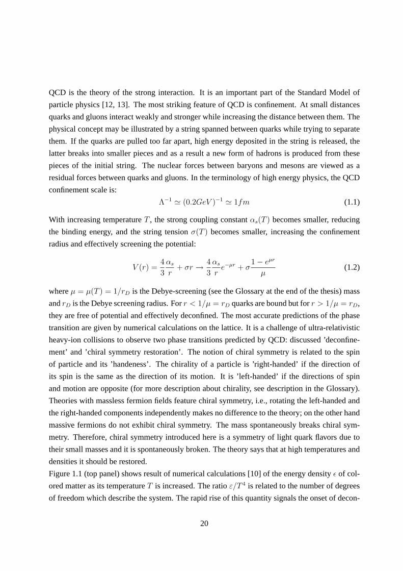
With increasing temperatureT , the strong coupling constantαs(T ) becomes smaller, reducing

the binding energy, and the string tensionσ(T ) becomes smaller, increasing the confinement

radius and effectively screening the potential:

V (r) =4

3

αs

r+ σr → 4

3

αs

re−µr + σ

1 − eµr

µ(1.2)

whereµ = µ(T ) = 1/rD is the Debye-screening (see the Glossary at the end of the thesis) mass

andrD is the Debye screening radius. Forr < 1/µ = rD quarks are bound but forr > 1/µ = rD,

they are free of potential and effectively deconfined. The most accurate predictions of the phase

transition are given by numerical calculations on the lattice. It is a challenge of ultra-relativistic

heavy-ion collisions to observe two phase transitions predicted by QCD: discussed ’deconfine-

ment’ and ’chiral symmetry restoration’. The notion of chiral symmetry is related to the spin

of particle and its ’handeness’. The chirality of a particleis ’right-handed’ if the direction of

its spin is the same as the direction of its motion. It is ’left-handed’ if the directions of spin

and motion are opposite (for more description about chirality, see description in the Glossary).

Theories with massless fermion fields feature chiral symmetry, i.e., rotating the left-handed and

the right-handed components independently makes no difference to the theory; on the other hand

massive fermions do not exhibit chiral symmetry. The mass spontaneously breaks chiral sym-

metry. Therefore, chiral symmetry introduced here is a symmetry of light quark flavors due to

their small masses and it is spontaneously broken. The theory says that at high temperatures and

densities it should be restored.

Figure 1.1 (top panel) shows result of numerical calculations [10] of the energy densityǫ of col-

ored matter as its temperatureT is increased. The ratioε/T 4 is related to the number of degrees

of freedom which describe the system. The rapid rise of this quantity signals the onset of decon-

20

finement above some critical temperatureTc. A relatively sharp deconfinement transition occurs

at a temperature of approximately 175 MeV in 2-flavor QCD and below this temperature quarks

and gluons are confined inside hadrons, so only protons and neutrons can be taken into account

to describe system. At higher temperatures more degrees of freedom have to be considered.

The most familiar example of phase transitions is the ’phasediagram’ of water, where controlled

parameters are temperatureT and pressurep. Water is commonly described as having three

phases: gas, liquid, and solid. There, a dependencep(T ) describes the transition from one phase

to another (solid to liquid and liquid to gas), which transition depends on pressure and tempera-

ture.

Two energy regimes are discussed for the QGP state and phase transitions: at lower energies,√

sNN ≃ 5− 20 GeV, typical for the AGS (BNL) and SPS (CERN) programs, the nuclei are ex-

pected to stop each other, leading to baryon-rich systems; this is the regime of maximum baryon

density. At higher energies,√

sNN ≥ 100 − 200 GeV, nuclei become more transparent and nu-

clear fragments are better separated from the central region of particle production at mid-rapidity.

This regime (baryon chemical potentialµB = 0) is expected to be baryon-free, or QGP (pure

QGP regime); high-energy experiments consider it as a region of "less-baryon density".

In the bottom panel of Figure 1.1 a schematic phase diagram isshown. The phase of matter de-

scribes the system in given regions of temperatureT andµB. Low temperatures andµB ≃ 940

MeV characterize ordinary nuclear matter. As the temperature and energy density are increased

further, transitions to deconfinement phases of quarks and gluons are expected to occur; these

are indicated by the lines in the plot.

A phase transition is characterized by its ’order’, corresponding to the order of the derivative of

the thermodynamical potential:

Ω(E, T, S, µc, N) = E − T · S − µc · N (1.3)

whereE means energy,T is the temperature,S is entropy,µc is chemical potential andN is the

number of particles. For the system in question, the formula1.3 is rewritten in the form:

Ω(E, T, S, µB, B) = E − T · S − µB · B (1.4)

whereµB is defined as the chemical baryon potential andB is the baryon number. Thermody-

namic equilibrium is reached whereΩ has a minimum. The phase transitions were labeled by

the lowest derivative of the free energy that is discontinuous at the transition. ’First-order’ phase

transitions exhibit a discontinuity in the first derivativeof the free energy with a thermodynamic

21

variable. The various solid/liquid/gas transitions are classified as first-order transitions because

they involve a discontinuous change in density (which is thefirst derivative of the free energy

with respect to chemical potential.) ’Second-order’ phasetransitions have a discontinuity in a

second derivative of the free energy. These include the ferromagnetic phase transition in mate-

rials such as iron, where the magnetization, which is the first derivative of the free energy with

the applied magnetic field strength, increases continuously from zero as the temperature is low-

ered below the Curie temperature. The magnetic susceptibility, the second derivative of the free

energy with the field, changes discontinuously. Under the Ehrenfest classification scheme, there

could in principle be third, fourth, and higher-order phasetransitions. In this case there is no dis-

continuity and no rapid phase transition, but a ’cross-over’. The solid line in Figure 1.1 indicates

a first-order phase transition at larger values of chemical potentialµB ≥ 360 ± 40 MeV with a

critical ’endpoint’ indicated by the small square, followed a smooth crossover forµB ≤ 360MeV.

As we know from the top panel of Figure 1.1, lattice QCD predicts a phase transition around the

critical temperatureTc = 175 ± 15 MeV. The order of the transition of the QGP phase is not

known. If gluons were the only degrees of freedom, the transition would be first-order. With

the addition of two or three quarks, the transition can be of second-order. At high temperature

and high baryon potential, lattice QCD results seem to indicate that the transition is a smooth

’cross-over’. Furthermore, there might be a second-order transition at high density, as shown in

Figure 1.1 (top panel). In the early universe, the QGP is thought to have existed10−4 − 10−5 s

after the Big Bang.

1.2 Relativistic heavy-ion collisions

As discussed in the previous section, collisions of heavy ions, like S, Au or Pb at relativistic

energies can produce a large and hot system where the QGP can be created. A pictorial view

of relativistic heavy-ion collisions is presented in Figure 1.2. In the center-of-mass system of

a symmetric nucleus-nucleus collision, two Lorenz-contracted nuclei of radiusR hit each other

along the beam axis with impact parameter−→|b| = b (where

−→b is perpendicular to the beam

direction the vector connecting centers of colliding nuclei). In the region of overlapping, the

’participating’ nucleons interact with each other, while in non-overlapping region, the ’spectator’

nucleons continue along their trajectories (but they can interact electromagnetically only). The

degree of overlap is called ’centrality of the collision’, with b ∼ 0 fm for the most central

collisions (total overlapping of two nucleons) andb ∼ 2R for the most peripheral collisions (no

overlapping area). The maximum time of overlapping is determined asτ0 = 2R/γc, whereγ is

22

Figure 1.2: The scheme ofAu + Au heavy-ion collision with radius R and the impact parameterb. The curve represents the relative probability of charge particle multiplicity nch, which isproportional to the number of participating nucleonsNpart[2].

the Lorenz factor if the colliding nuclei.

The impact parameter of a collision in the case of gold nucleiis directly related to the number of

participantsNpart, where in the most central collisions it can reach up to 394 nucleons and in the

most peripheral collisions the number of participants can be very small. The beam axis and the

direction of impact the impact parameter define a reaction plane.

The colliding nuclear matter loses a substantial fraction of its energy in the collision process, a

phenomenon referred to by the therm ’nuclear stopping power’ introduced by Busza and Gold-

haber [14]. The loss of kinetic energy incident nuclear matter is accompanied by the production

of a large number of particles, mostly pions. Therefore, in high-energy collisions, a large frac-

tion of the longitudinal energy is converted into the energyof hadronic matter produced in the

neighborhood of the center of mass of the colliding system.

The dynamics of a heavy-ion collision can be viewed in Figure1.3 as a space-time diagram with

the longitudinal coordinatez and and the time coordinatet. The collision takes place at the point

(z, t) = (0, 0). The space-time scenario proposed by Bjorken [15], distinguishes five sub-sequent

23

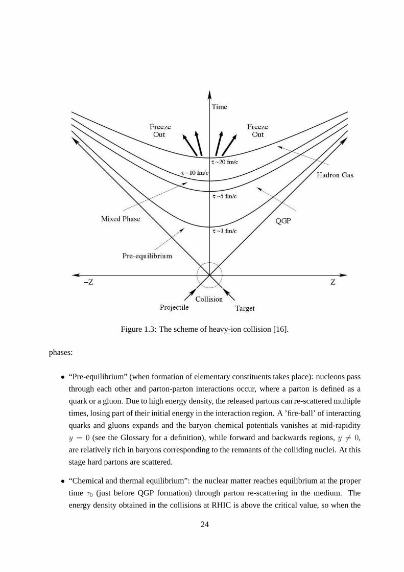
Figure 1.3: The scheme of heavy-ion collision [16].

phases:

• “Pre-equilibrium” (when formation of elementary constituents takes place): nucleons pass

through each other and parton-parton interactions occur, where a parton is defined as a

quark or a gluon. Due to high energy density, the released partons can re-scattered multiple

times, losing part of their initial energy in the interaction region. A ’fire-ball’ of interacting

quarks and gluons expands and the baryon chemical potentials vanishes at mid-rapidity

y = 0 (see the Glossary for a definition), while forward and backwards regions,y 6= 0,

are relatively rich in baryons corresponding to the remnants of the colliding nuclei. At this

stage hard partons are scattered.

• “Chemical and thermal equilibrium”: the nuclear matter reaches equilibrium at the proper

time τ0 (just before QGP formation) through parton re-scattering in the medium. The

energy density obtained in the collisions at RHIC is above thecritical value, so when the

24

interacting medium is thermalized, the QGP might be produced.

• The ”QGP phase”, evolving according to the laws of hydrodynamics.

• The ”Mixed phase” of QGP and a Hadron Gas (HG)

• “Hadronization and freeze-out”: The expanding QGP cools down fast and quickly reaches

the transition temperature. It evolves into the phase of hadron gas, finally reaching the state

known as ‘chemical freeze-out’. The resulting hadronic gascontinues to expand, cooling

down the interaction rate between the hadrons. Then the system evolves to the thermal

equilibrium; this state is known as ‘thermal freeze-out’. After this moment, hadrons fly

freely.

Information about the QGP or the hadron gas at thermal equilibrium must be inferred from

the properties of the particles remaining after the thermalfreeze-out (hadrons, leptons, direct

photons). Some signatures described in Section 2 can give information about what happened

before the freeze-out.

25

Chapter 2

Properties of bulk matter - review of

experimental results

The RHIC facility (more in Chapter 5) enables probing the highest-energy region of phase space,

where many processes are subjects of our interest. The processes detected in the RHIC energy

domain can be selected according to many criteria, one of them being dividing experimental ob-

servables into the ‘soft’ and ‘hard’ sector of processes. Particle production in the central rapidity

region of ultra-relativistic heavy-ion collisions can be treated as a combination of perturbative

(hard and semi-hard) parton production and non-perturbative (soft) particle production. By ’hard’

one usually means clearly perturbative processes with momentum or mass scale of the order of

tens of GeV. The resulting hard partons can fragment into jets. Hadronic jets are observed inp+p

collisions at thepT from around 5 GeV to more than 400 GeV. The term ‘Semi-hard’ processes

refers to such QCD process where partons with transverse momenta of few GeV are produced.

’Soft’ process refers, to ones which produce low transversemomenta partons or hadrons.

2.1 Soft processes

2.1.1 Inclusive and semi-inclusive particle production - thermal equilib-

rium signatures

Single particle distributions are used to look into particle production mechanisms and deduce

information concerning system evolution. Measurements inthe left panel of Figure 2.1 are pre-

26

Figure 2.1: a) Semi-inclusive invariantpT spectra for pions, kaons and protons inAu + Aucollisions at

√sNN = 200 GeV. Left column contains positive hadrons and right one negative

particle species. Top row shows the sample of the most central collisions (up to 5% of thetotal hadronic cross-section of the collision) and the bottom row indicates the most peripheralcollisions (from 60 to 92% of the cross-section). b) mean transverse momentum of positiveparticles as a function of centrality [17].

sented in terms of Lorentz invariant single particle inclusive differential cross-section (or Yield

per event in the class of semi-inclusive):

Ed3σ

dp3=

d3σ

pT dpT dydφ=

1

2πf(pT , y) (2.1)

wherey is rapidity (see Glossary for a definition),pT is transverse component of the momentum

vector−→p , (while pL is the longitudinal component of momentum),σ is the cross section of a

reaction andφ is the azimuthal angle of the particle.

The plot exhibits some differences between distributions (of pions, kaons and protons) for

various centralities (mainly in the number of produced particles of a given type), however their

shapes do not differ significantly. The distributions are usually used to estimates the temperature

27

of thermal freeze-out, as:

d2σ

dpLpT dpT

=d2σ

dpLmT dmT

=1

eE/T ± 1∼ e−E/T (2.2)

The slope of themT (or pT ) distribution at mid-rapidity represents temperature of the system.

Particles (or partons) which travel with transverse flow velocity βt = vt

cacquire kinetic energy

in addition to thermal energy, so the slope should increase with the rest mass:T → T0 + γT m0.

The average transverse momentum< pT > of positive pions, kaons and protons (see right

panel of Figure 2.1) increases according to their respective masses. The rise of mean transverse

momentum of hadrons from peripheral to central collisions is expected for thermal distributions.

2.1.2 Chemical equilibrium signatures

One of the most crucial questions is whether thermal and chemical equilibrium is achieved at

some stage of the collision. Applying a statistical model [18, 19] which assumes equilibrium,

and testing the experimental data against model predictions is one way to verify if the equilibrium

state was reached during systems evolution. The statistical model is based on the use of a grand

canonical ensemble to describe the partition function and hence the density of the particles in a

equilibrated fireball:

ni =gi

2π2

∫

∞

0

p2dp

e(Ei(p)−µi)/T ± 1(2.3)

with particle densityni, spin degeneracygi, ~ = c = 1, momentump, total energyE and

chemical potentialµi = µBBi − µSSiµI3I3i . i denotes particle type. The quantitiesBi, Si and

I3i are the baryon number, strangeness and three-component of the isospin quantum number.

The temperatureT and baryon-chemical potential of chemical freezeout are the two independent

parameters of the model, while the volume of the fireballV , the strangeness chemical potential

µS and the isospin chemical potentialµI3 are fixed by the three conservation laws:

V∑

i

niBi = Z + N (2.4)

V∑

i

niS = 0 (2.5)

28

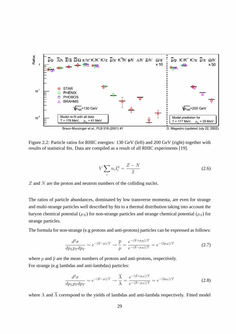
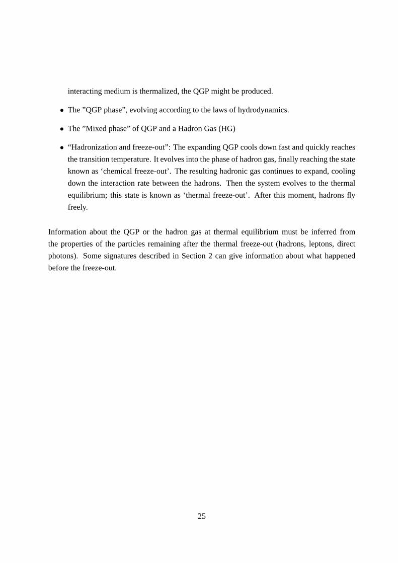
Figure 2.2: Particle ratios for RHIC energies: 130 GeV (left)and 200 GeV (right) together withresults of statistical fits. Data are compiled as a result of all RHIC experiments [19].

V∑

i

niI3i =

Z − N

2(2.6)

Z andN are the proton and neutron numbers of the colliding nuclei.

The ratios of particle abundances, dominated by low transverse momenta, are even for strange

and multi-strange particles well described by fits to a thermal distribution taking into account the

baryon chemical potential (µB) for non-strange particles and strange chemical potential(µS) for

strange particles.

The formula for non-strange (e.g protons and anti-protons)particles can be expressed as follows:

d2σ

dpLpT dpT

∼ e−(E−µ)/T → p

p=

e−(E+µB)/T

e−(E−µB)/T= e−(2µB)/T (2.7)

wherep andp are the mean numbers of protons and anti-protons, respectively.

For strange (e.g lambdas and anti-lambdas) particles:

d2σ

dpLpT dpT

∼ e−(E−µ)/T → Λ

Λ=

e−(E+µS)/T

e−(E−µS)/T= e−(2µS)/T (2.8)

whereΛ andΛ correspond to the yields of lambdas and anti-lambda respectively. Fitted model

29

Figure 2.3: a) pseudorapidity distributions forAu + Au at 200 GeV for different collision cen-tralities; b) multiplicity of charged particles per participant pair around midrapidity as a functionof collision energy. Particle production inAu + Au collision at top RHIC energies aroundη = 0exceeds that seen inp + p collisions by40 − 50% [20].

parameters (temperature, baryon potential of the chemicalfreezeout) from the thermal distribu-

tion are displayed in Figure 2.2. For√

sNN = 130 GeV, the temperature isT = 176 MeV and

the chemical potential-µB = 41 MeV, for√

sNN = 200 GeV,T = 177 MeV andµB = 29 MeV.

These calculations are done to estimate in which region of the phase diagram the analyzed sys-

tem is located. These predictions agree with QCD calculations and confirm the fact that RHIC

experiments access the region located very close to the boundary of the phase transition.

2.1.3 The (pseudo-)rapidity density

The reference frame of the detectors at RHIC is designed to be anucleon-nucleon center of

mass (c.m.) system. The colliding nucleons approach each other with the energy√

sNN/2.

The rapidity of the nucleon-nucleon center of mass - mid-rapidity - is ycm = yNN = 0. The

projectile’s and target’s rapidities are equal (in absolute magnitude), but have opposite signs:

yproj = −ytarget = cosh−1(

√sNN

2mN

) = ybeam/2 (2.9)

30

Figure 2.4: Baryon ratios for RHIC and SPS energies showing thenet baryon density for somebaryon species at given collision energy. Open symbols are for the energy of SPS, closed symbolsshow RHIC results [18].

wheremN=0.931 GeV is the mass of nucleon andybeam means the beam rapidity. The shape

and evolution of charged-particle density in rapidityy and pseudorapidity (η = −ln[tan(0.5θ)],

whereθ is the angle of particle with respect to the beam axis) inA + A collisions (see Figure

2.3) follow a similar trend. Pseudorapidity is calculated in the case where rapidity cannot be

measured directly, for the central-rapidity region rapidity and pseudorapidity distributions follow

very similar trends. For more central data, higher multiplicities of particles are registered. The

event multiplicity is collision energy-dependent as well (right-hand side of Figure 2.3). Universal

scaling of pseudo-rapidity divided by the number of collision participants versus collision energy

is observed.

2.1.4 “Net” baryon density

The anti-baryon/baryon ratios have been measured at the SPSand RHIC Displayed in Figure 2.4

are the ratios for SPS (open symbols) and RHIC energies (closed symbols) slightly increase with

increasing the content of strange quark of the observed anti-baryon/baryon ratios. Obviously,

there is a large increase of baryon ratios from lower to higher energies due to much higher

baryon density for higher energy (at lower energies production of anti-baryons was limited). The

31

tendency for both energies are similar. The slight increaseof ratios (such exists in collisions

of two nuclei) for both energies is a result of an increase of strange quark content (see the next

sub-section for more details about strangeness production). This measurement indicates that

baryon-rich density is strange quark content-dependent.

2.1.5 Strangeness Recombination

Strangeness enhancement was one of the first proposed signals for the possible QGP formation

[21]. The strangeness content of the colliding nuclei is negligible, consequently all measured

strange particles must have been produced during collision. The strange quarks has a much

larger mass than lighter quarks (u, d), as described in Appendix 1. The production of particles

containing thes quark through hadronic channels usually should not be enhanced. Asms < Tc,

an (ss) pair would be in chemical and thermal equilibrium in the QGP phase. Strange quarks

would hadronize, resulting in an enhancement of productionof strange particles (containing at

least one strange quark or anti-quark). Hyperon production(where hyperon is a baryon with

at least one strange or anti-strange quark) in a collision ofhadron is expected to be more diffi-

cult for multi-strange species (Ξ, Ω), which usually result from a long cascade of reactions, e.g:

π + N → K + Λ, π + Λ → Ξ + K, π + Ξ → Ω + K. (See also [22]).

In this section, two experimental results are presented: the dependence of strange particle pro-

duction as a function of the thes quark content in a hyperon and the relation of strange quarksto

non-strange light ones (u, d).

It is expected that more hyperons may be detected when a QGP phase is created than in the case

of a pure-hadronic system. This effect should increase withthe strangeness content of the baryon.

The SPS experiment NA57 [23] has measured the yields ofΛ, Λ,Ξ±, Ω± in p + A andA + A

collisions. These results are compared as a function of the number of participating or wounded

nucleons. Figure 2.5 presents the ratio of (anti)-hyperon yield in nucleus-nucleus (A + A) col-

lisions to thep + Be andp + p ones, versus the number of participants (centrality) measured

at SPS conditions and extended to the RHIC energy domain. If the yields were simply scaling

with the number of participants then all points should be distributed on a flat line. This figure

indicates an enhancement of production of (anti)-hyperonswith the centrality of the collision.

The second important point here is the hierarchy of enhancement- it is higher for multi-strange

baryons (Ω, Ξ) than for single strange baryons (Λ) leading to the conclusion than if thes quark

content in a particle is higher, then the production of such hadron increases.

As the strangeness content in hadronic matter and in QGP is different, information about pro-

32

Figure 2.5: Ratio of yields of (anti)-hyperons versus centrality measured forA + A collisionswith respect top + p (STAR) andp + Be (NA57) at SPS (closed symbols) and RHIC (openedsymbols). Lambda hyperons are marked by black circles, sigma particles are shown by redsquares and omegas are plotted as blue triangles [24].

33

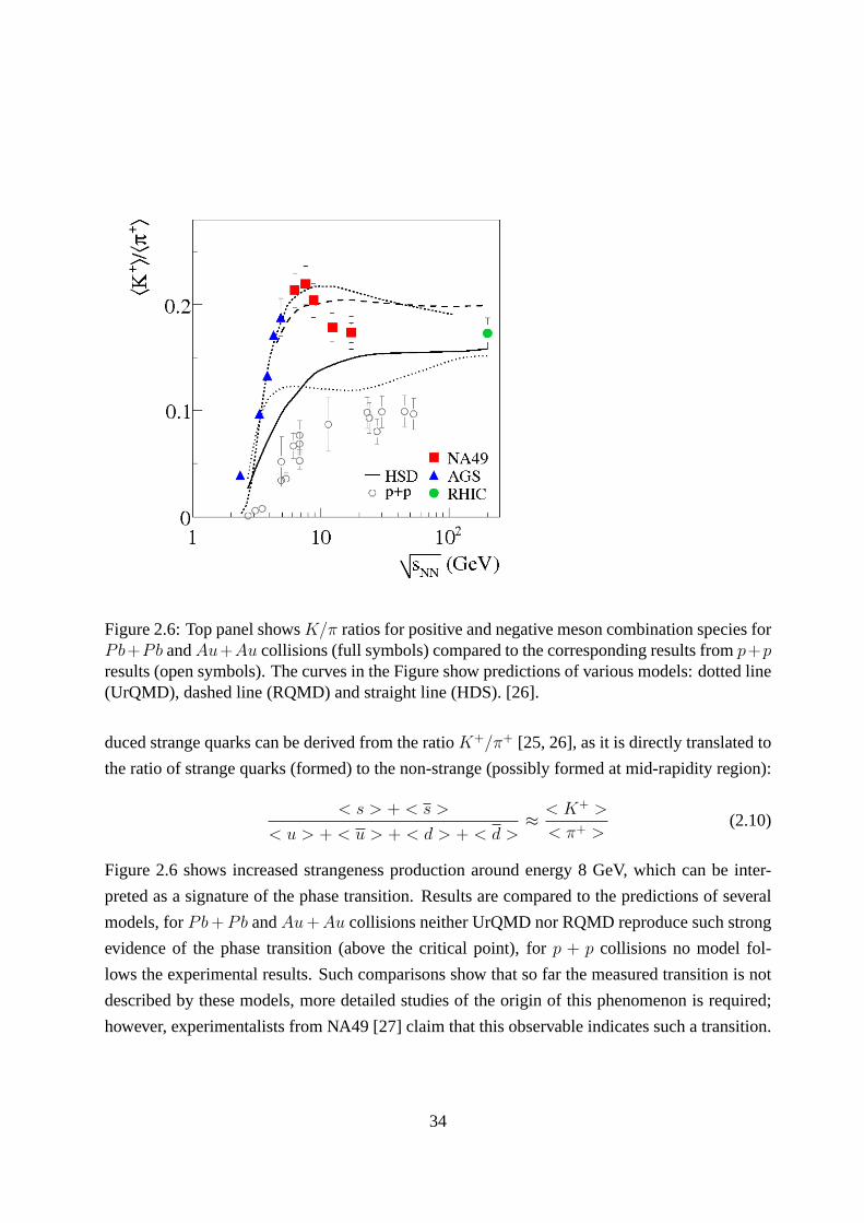
Figure 2.6: Top panel showsK/π ratios for positive and negative meson combination speciesforPb+Pb andAu+Au collisions (full symbols) compared to the corresponding results fromp+presults (open symbols). The curves in the Figure show predictions of various models: dotted line(UrQMD), dashed line (RQMD) and straight line (HDS). [26].

duced strange quarks can be derived from the ratioK+/π+ [25, 26], as it is directly translated to

the ratio of strange quarks (formed) to the non-strange (possibly formed at mid-rapidity region):

< s > + < s >

< u > + < u > + < d > + < d >≈ < K+ >

< π+ >(2.10)

Figure 2.6 shows increased strangeness production around energy 8 GeV, which can be inter-

preted as a signature of the phase transition. Results are compared to the predictions of several

models, forPb + Pb andAu + Au collisions neither UrQMD nor RQMD reproduce such strong

evidence of the phase transition (above the critical point), for p + p collisions no model fol-

lows the experimental results. Such comparisons show that so far the measured transition is not

described by these models, more detailed studies of the origin of this phenomenon is required;

however, experimentalists from NA49 [27] claim that this observable indicates such a transition.

34

2.1.6 Flow

The flow phenomenon is a distinguishing feature of a nucleus-nucleus collision compared to the

simpler ones: proton-proton or proton-nucleus [28, 29, 30]. This effect is seen at many collision

energies. Flow is a collective effect of a bulk matter which obviously cannot be produced as a

result of superposition of independent nucleon-nucleon collisions. There can be isotropic or non-

isotropic expansion, depending on the class of the collision centrality. Depending on the collision

energy, flow does reflect different collective aspects of theinteracting medium. At low energies,

where relatively few new particles are formed, the flow effect is mostly caused by nucleons from

the incoming nuclei. At higher energies, the number of newlyproduced particles is so large that

they dominate the observed flow effect; the primordial nucleons are expected to make only minor

contribution, in particular in the region of mid-rapidity.

• Radial flow

In central collisions between spherical nuclei, the initial state is symmetric in azimuth and

the overlapping region is circular (not ’almond-shape’ in the transverse direction); this

implies that the azimuthal distribution of the final state particles is isotropic as well. Under

such conditions, any pressure gradient causes azimuthallysymmetric collective flow of the

outgoing particles, which is called ‘radial flow’. The relevant observables to study such

effects are the transverse momentum distributions for various particle species. For a given

particle type, the random thermal motion is superimposed onto the collective radial flow

velocity.

• Anisotropic flow

Here non-central collisions are discussed, where the pressure gradient is not azimuthally

symmetric. The pressure gradient establishes a correlation between momentum and po-

sition points. The initial anisotropy in the transverse space configuration translates into

an anisotropy of the transverse momentum distributions of outgoing particles, which is

refereed to as ‘anisotropic flow’. It depends on collision energy, location in phase space

(rapidity, transverse momentum) and the particle species.The dominating flow pattern at

low energies arises from colliding nuclei. In such a case, the flow from the projectile nuclei

must have its maximum in the reaction plane. Furthermore, the flow of particles originat-

ing from the target is characterized by the same magnitude, than the flow of the projectile

remnants from opposite direction. The collective motion iscalled ‘directed flow’ and it

can be large at low energies. The velocity of incoming nucleiat ultra-relativistic energies

35

Figure 2.7: a) almond shaped overlap region just after nucleus-nucleus collision, where the nucleimove alongz axis, the reaction plane is defined by thez and x axis (defined by the impactparameter vector); b) The view of the collision and momentumdistribution just after collision[2].

is the biggest in the longitudinal direction, so the flow exists rather in this direction than in

the transverse plane. As a result, the directed flow is significantly reduced at high energies.

As most particles are produced in the interaction volume, they can exhibit additional flow

patterns. The momentum of these particles can be viewed in the transverse plane as an

ellipse with the principal axes parallel and perpendicularto the reaction plane. The corre-

sponding dominant flow is called ‘elliptic flow’.

The overlap region in nucleus-nucleus collisions is definedby the nuclear geometry and is al-

mond shaped. The single particle spectrum is modified by an expansion of the particle with

respect to the reaction planeφ − ΦR, whereφ is the azimuth of the particle, andΦR is the angle

of the reaction plane defined along the impact parameter vector (x axis in Figure 2.7):

Ed3N

dp3=

d3N

pT dpT dydφ=

d3N

2πpT dpT dy[1 + 2υ1cos(φ − ΦR) + 2υ2cos2(φ − ΦR) + ...] (2.11)

The coefficientυ1 reflects the ’directed flow’ andυ2- the ’elliptic flow’. If the thermal equilibrium

is reached, the pressure gradient is directed mainly along the direction of the impact parameter

vector and collective flow develops along this direction.

36

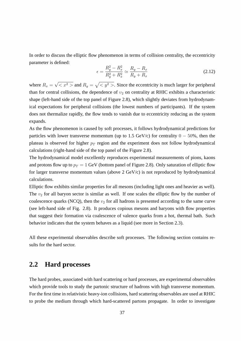
In order to discuss the elliptic flow phenomenon in terms of collision centrality, the eccentricity

parameter is defined:

ǫ =R2

y − R2x

R2y + R2

x

≃ Ry − Rx

Ry + Rx

(2.12)

whereRx =√

< x2 > andRy =√

< y2 >. Since the eccentricity is much larger for peripheral

than for central collisions, the dependence ofυ2 on centrality at RHIC exhibits a characteristic

shape (left-hand side of the top panel of Figure 2.8), which slightly deviates from hydrodynam-

ical expectations for peripheral collisions (the lowest numbers of participants). If the system

does not thermalize rapidly, the flow tends to vanish due to eccentricity reducing as the system

expands.

As the flow phenomenon is caused by soft processes, it followshydrodynamical predictions for

particles with lower transverse momentum (up to 1.5 GeV/c) for centrality0 − 50%, then the

plateau is observed for higherpT region and the experiment does not follow hydrodynamical

calculations (right-hand side of the top panel of the Figure2.8).

The hydrodynamical model excellently reproduces experimental measurements of pions, kaons

and protons flow up topT = 1 GeV (bottom panel of Figure 2.8). Only saturation of elliptic flow

for larger transverse momentum values (above 2 GeV/c) is notreproduced by hydrodynamical

calculations.

Elliptic flow exhibits similar properties for all mesons (including light ones and heavier as well).

Thev2 for all baryon sector is similar as well. If one scales the elliptic flow by the number of

coalescence quarks (NCQ), then thev2 for all hadrons is presented according to the same curve

(see left-hand side of Fig. 2.8). It produces copious mesonsand baryons with flow properties

that suggest their formation via coalescence of valence quarks from a hot, thermal bath. Such

behavior indicates that the system behaves as a liquid (see more in Section 2.3).

All these experimental observables describe soft processes. The following section contains re-

sults for the hard sector.

2.2 Hard processes

The hard probes, associated with hard scattering or hard processes, are experimental observables

which provide tools to study the partonic structure of hadrons with high transverse momentum.

For the first time in relativistic heavy-ion collisions, hard scattering observables are used at RHIC

to probe the medium through which hard-scattered partons propagate. In order to investigate

37

Figure 2.8: Top-left: elliptic flow of charged particles near midrapidity (|η| < 1) as a functionof centrality inAu + Au collisions at

√sNN = 200 GeV, with systematic errors; smooth curve

corresponds to the hydrodynamical predictions close to thecalculation with fixedυ2/ε = 0.25[31]. Top-right: elliptic flow of charged particles for midrapidity region in 50% of the mostcentral collisions [31]; bottom right: transverse momentum dependence of elliptic flow for pions,kaons and protons measured by STAR, together with hydrodynamical calculations [29], bottom-left: elliptic flow scaled by NCQ for mesons and baryons [32].

38

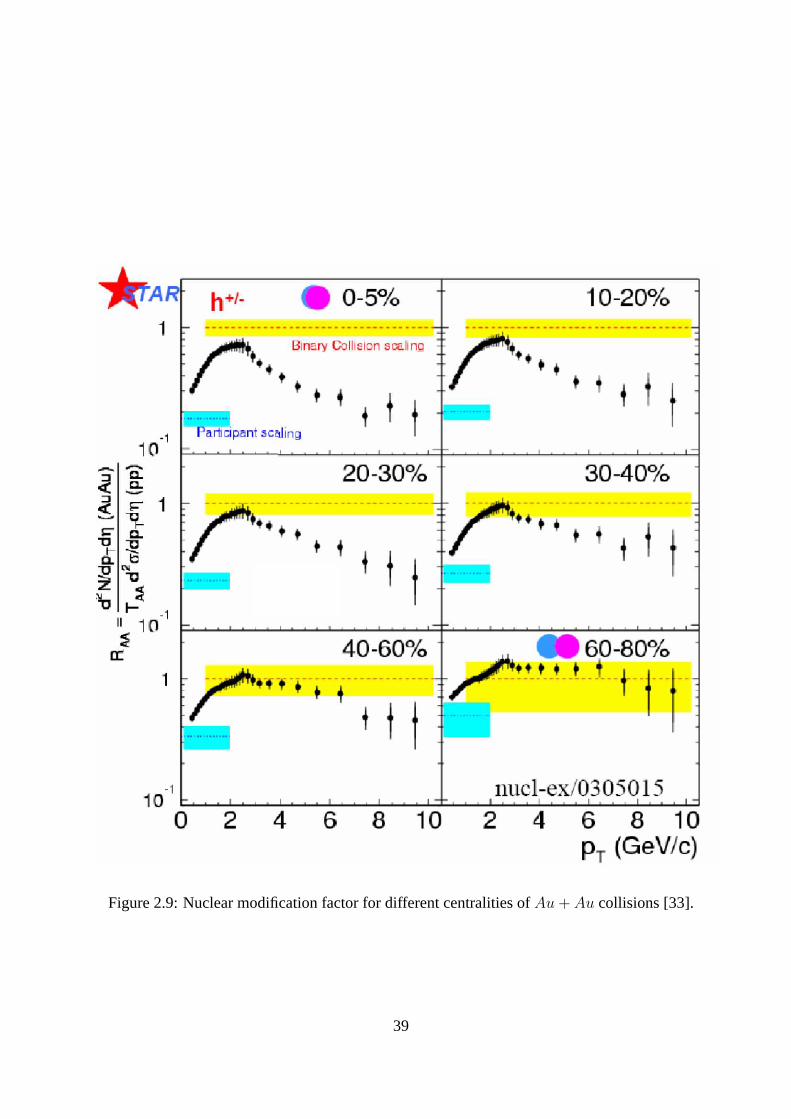
Figure 2.9: Nuclear modification factor for different centralities ofAu + Au collisions [33].

39

Figure 2.10: Nuclear modification factor for centralAu + Au collisions.d + Au data is shownas well [33].

parton energy loss, the RHIC experiments measure hadron spectra and azimuthal correlations of

particles with highpT .

2.2.1 Jet quenching

Jet quenching was proposed as a signature of QGP in the RHIC energy domain. It is expected

to be stronger in higher energy collisions of heavy-ions (e.g. in ALICE experiment at the LHC

accelerator). In the initial collision of two nuclei, hard scatterings can occur which produce pairs

of outgoing particles with high momentum. If the medium is dense, which takes place often in

the case of nucleus-nucleus collision, where large numbersof particles are produced, partons

lose their energy, which leads to the reduction of theirpT . In other words, when partons move

through dense medium, they lose their energy as a result of gluon radiation.This phenomenon is

called ’jet quenching’.

In order to compare various colliding systems one can calculate the ’nuclear modification factor’

usingp + p as a reference toA + A:

RAA(pT ) =

(

d2NAA

dydpT

)

/

(

Ncolld2Npp

dydpT

)

(2.13)

40

whereNcoll is the number of binary collisions in the heavy-ion system,NAA andNpp are the

average numbers of particles produced in, respectivelyA + A (nucleus-nucleus, e.g.Au + Au)

andp + p collisions,y is the rapidity. Sometimes, the nuclear modification factoris expressed in

terms:

RCP (pT ) =

(

Nperipheralcoll

d2N centralAA

dydpT

)

/

(

N centralcoll

d2NperipheralAA

dydpT

)

(2.14)

whereNperipheralcoll andN central

coll are the numbers of collisions, andN centralAA andNperipheral

AA are the

average numbers of produced particles, respectively in central and peripheral collisions.

WhenRAA = 1 such anA+A collision is a superposition ofN−N (nucleon-nucleon) collisions

corresponding to scaling with the number of binary collisions (binary scaling). Suppression of

the hadron spectra is observed by the nuclear modification factor measured in centralAu + Au

collisions at RHIC. Figure 2.9 depictsRAA as a function ofpT for 6 different centrality classes

for Au + Au collisions. The ratios are taken relatively top + p collisions scaled by the number

of binary collisions. The data expresses clear suppressionby a factor of 4-5 in the central case

at large transverse momentapT > 2 GeV/c . The distributions for peripheral collisions remain

rather flat up to thepT about 10 GeV/c. As the jet quenching phenomenon is strongly dependent

on medium density, it is clearly reflected by the centrality dependence of nuclear modification

factor. As in central collisions the produced medium is muchdenser than in peripheral collisions,

jet quenching should appear stronger in central ones. TheRdAu are not suppressed (Figure 2.10)

what indicates different medium properties than inAu+Au collisions. Figure 2.11 illustrates, the

jet quenching effect shown together for four RHIC experiments: left-hand side of the top panel is

dedicated to the PHENIX Collaboration, which shows nuclear modification factor forAu + Au

collisions for charged hadrons and neutral pions produced separately (not suppressed data); right-

hand side of the top panel showsRdAu for two class of collision centrality (not suppressed data

as well) by the PHOBOS Collaboration; left-hand side of the bottom panel presents nuclear

modification factor ford + Au andAu + Au collisions by BRAHMS experiment (Au + Au data

suppressed andd + Au collisions not suppressed).

Another interesting observable of hadron production is two-particle azimuthal correlations. They

are calculated according the formula:

D(∆φ) =1

Ntrig

dN

d(∆φ)(2.15)

where the azimuthal separation is normalized by the number of triggered particlesNtrig, ∆φ rep-

resents the azimuthal angle. In order to calculate∆φ, one particle is chosen as a trigger and then

41

Figure 2.11: Nuclear modification factor measured by PHENIX(left-hand side of the top panel),PHOBOS (right-hand side of the top panel) and BRAHMS experiment(left-hand side of thebottom panel). Di-hadron azimuthal correlations at high transverse momentum. Sub-panel showscorrelations forp + p, centrald + Au andAu + Au from STAR [34]. See more description inthe text.

42

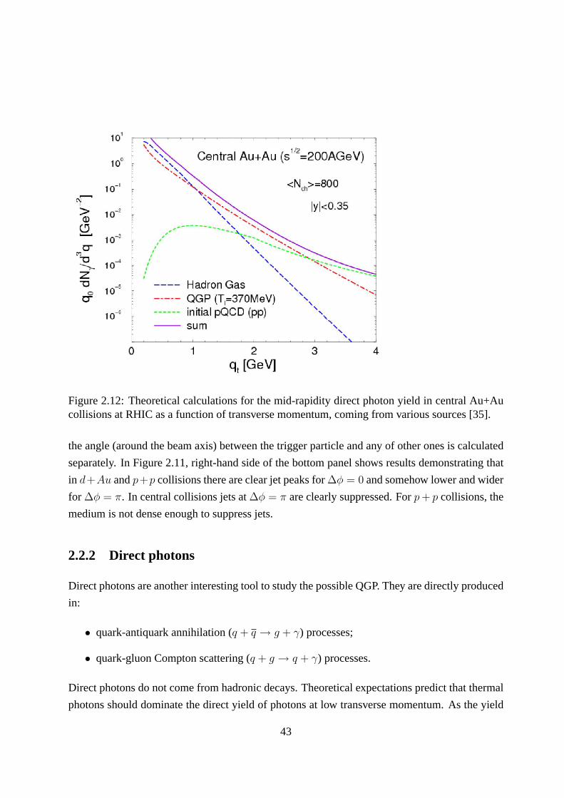
Figure 2.12: Theoretical calculations for the mid-rapidity direct photon yield in central Au+Aucollisions at RHIC as a function of transverse momentum, coming from various sources [35].

the angle (around the beam axis) between the trigger particle and any of other ones is calculated

separately. In Figure 2.11, right-hand side of the bottom panel shows results demonstrating that

in d+Au andp+p collisions there are clear jet peaks for∆φ = 0 and somehow lower and wider

for ∆φ = π. In central collisions jets at∆φ = π are clearly suppressed. Forp + p collisions, the

medium is not dense enough to suppress jets.

2.2.2 Direct photons

Direct photons are another interesting tool to study the possible QGP. They are directly produced

in:

• quark-antiquark annihilation (q + q → g + γ) processes;

• quark-gluon Compton scattering (q + g → q + γ) processes.

Direct photons do not come from hadronic decays. Theoretical expectations predict that thermal

photons should dominate the direct yield of photons at low transverse momentum. As the yield

43

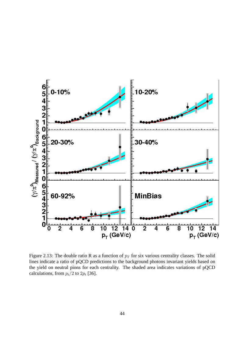
Figure 2.13: The double ratio R as a function ofpT for six various centrality classes. The solidlines indicate a ratio of pQCD predictions to the background photons invariant yields based onthe yield on neutral pions for each centrality. The shaded area indicates variations of pQCDcalculations, frompt/2 to 2pt [36].

44

of thermal photons fall off exponentially with transverse momentum, direct photons from the

initial hard scattering will dominate the spectrum at higher transverse momentum values (Figure

2.12). In addition, a contribution of photons produced during parton fragmentation is observed.

Measurements of thermal photons can provide information about temperature. Measurements of

prompt photons allow one to study properties of jets interacting with the medium. They also are

interesting in that they could provide background for thermal components.

The production of prompt photons is represented by the nuclear modification factor with yields

of hadrons inA+A collisions relative to the scaled reference measured inp+p collisions. Direct

photons provide a tool to check the binary collision scalingsince their production is not affected

by the medium produced in the final stage of the interaction. At RHIC energies it is possible to

study direct photons inAu+Au, d+Au andp+p collisions. Prompt photons inp+p collisions

provide an excellent test of QCD, while results fromd+Au collisions may be used to investigate

nuclear effects.

In order to determine direct photons, the following formulais calculated:

R =(γ/π0)measured

(γ/π0)decay

= 1 +γdirect

γdecay

(2.16)

where the numerator corresponds to measured inclusive photon spectrum of the neutral pion

spectrum and the denominator reflects the number of simulated decay photons per input pion,

shown in Figure 2.13. The contribution of direct photons increases with transverse momentum.

It is also collision centrality dependent, for more centraldata the number of direct photons ver-

sus number of decayed ones is bigger indicating that production for central data respectively

increases and decreases as collision is described by biggerimpact parameter.

2.2.3 Production of heavy flavors

For many years suppression of theJ/ψ resonance has been believed, according to lattice cal-

culations, simplificating to be a signature of QGP phase, asJ/ψ production in nucleus-nucleus

collisions should be suppressed by Debye screening processes. TheJ/ψ is produced when two

gluons interact to create a(cc) pair, which then form aJ/ψ resonance. As in QGP the(cc) in-

teraction can be screened, its quarks can take part in open-charm production processes (in other

words, they can create other hadrons than theJ/ψ resonance, e.g.D0 = cu, D0 = cu, B0 = db,

B0 = db, Υ = cb). The NA50 Collaboration [37] has seen a suppression ofJ/ψ in central

Pb + Pb collisions as√

sNN = 17.2 GeV. The suppression in order of 25% with respect to the

45

Figure 2.14: TheJ/Ψ yield normalized by Drell-Yan process versus transverse energy as mea-sured by NA50 in Pb+Pb collisions at SPS. Expectations from models assuming QGP formationare superimposed. Black curve corresponds to the predictions based on lighter systems (fromp+p to S+U collisions). Here, a decrease in the order of 25% isobserved. [38]

normal suppression in nuclear matter might be interpreted as an evidence for deconfined quarks

and gluons. Figure 2.14 shows the yield ofJ/ψ normalized by Drell-Yan processes. TheJ/ψ

measurements rely on the ratio of observedJ/ψ → µ+µ− decays over the number of Drell-Yan

processes (qq → µ+µ−). The ratios obtained experimentally are compared to the prediction of

absorption model, and different parts of the whole data sample taken by NA50 Collaboration are

consistent with each other.

Due to large production of charmed quarks, the suppression scenario changes at higher energies

like those available at RHIC. Experiments at RHIC study the behavior of this possible signature,

but from preliminary results at low statistics it cannot be concluded that the ratio of measured

to expected of producedJ/ψ particle is different than unity.J/Ψ suppression is seen at RHIC

energies as well, however its signature as a probe of QGP in lower energies is questionable and

cannot be treated as a clear probe of registration the deconfinement stage. In RHIC energy do-

46

main such suppression occurs for aΥ = bb particle. However, because of the small number of

bottomium pairs produce at RHIC,Υ formation by coalescence of unrelated pairs is negligible.

Because charm and bottom quarks are massive ones, they are produced almost exclusively in

the initial parton-parton interaction in heavy-ion collisions at RHIC energies. In the absence of

any nuclear effect, the heavy flavor cross-sections inA + A collisions at RHIC would simply

scale with the number of binary collisions. Thus departuresfrom binary scaling for heavy flavor

production inA + A collisions provide information about nuclear effects.

The easiest way to measure open heavy flavor yields in heavy-ion collisions at RHIC is through

semileptonic decays ofD andB mesons. Two very striking and unexpected results have been

seen by studying decay electrons from open heavy flavor at RHIC.The first is the observation

that the nuclear modification factor for electrons from openheavy flavor decays show very strong

suppression in centralAu+Au collision [39, 40], similar to that seen for pions. The second strik-

ing result is the elliptic flow of electrons from open heavy flavor decays appears to favor charm

quark at lowpT [40]. It was expected that heavy quark energy loss would be considerably smaller

than that for light quarks due to interference effect. The relatively largev2 values at low trans-

verse momentum imply at least some degree of charm quark equilibration with the medium. This

also imply very strong interactions of charm quarks with themedium at lowerpT .

However it is clear that the RHIC heavy flavor program is now limited by the capabilities of the

accelerator and the detectors. The accelerator upgrades planned over the period 2009-2013 to

produce a factor of5 greater luminosity at RHIC II, combined with the detector upgrades will be

required for the heavy flavor program at RHIC.

2.3 Perfect Liquid

On one hand, theoretical predictions have assumed that in the case of creation the QGP phase,

it should reflect properties of ideal gas. On the other hand, one of the most thrilling of exper-

imental results obtained at RHIC is the ’superstrong’ quenching of jets. While quenching was

expected and considered by many as a signal of the formation of QGP, it was not expected to

be so strong. This fact combined with the robust flow effects observed in the same reactions

and which confirmed the hydrodynamical nature of matter leadto the conclusion that the RHIC

experiments are very close to the QGP phase, but its behaviordoes not reflect properties of ideal

gas, but of ideal fluid; the observed system is a very stronglyinteracting one, thus called ’sQGP’

[41]. These measurements indicate that hydrodynamics describes heavy-ion collisions, and the

following system evolution surprisingly well, even if it fails in describing of many observables

47

(e.g spectra, HBT- see more in Chapter 5), but reproduces otherobservables well if earlier ther-

malization is assumed.

Measurements and comparison with relativistic hydrodynamic models indicate that the matter

thermalizes in unexpectedly short time, has an energy density at least15 times larger than needed

for color confinemen, has a temperature about twice the critical temperature predicted by lattice

QCD, and appears to exhibit collective motion with ideal hydrodynamical properties- a "perfect

liquid" that appears to flow with a near-zero viscosity to entropy ratio- lower than any previously

observed fluid nd perhaps close to a universal lower bound. However, a fundamental understand-

ing of the medium seen in heavy-ion collisions at RHIC does notyet exist. The most important

scientific challenge for the field in the next decade is the quantitative exploration of the new state

of nuclear matter.

The next section contains a description of two models applied successfully in heavy-ion physics

in order to compare experimental observables to theoretical predictions.

48

Chapter 3

Heavy-ion Collision Models

A complicated process of particle production can be described using theoretical models. Nowa-

days there exist two main descriptions based on: QCD string breaking and QCD parton cascade.

In the case of the string decay picture, the nuclei pass through each other and as a result of

their collision, color strings are formed. A string can be depicted as a quark - anti-quark pair

connected by the color field. In the next step, the string decays producing hadrons, quarks

and gluons. Most known descriptions based on string fragmentation are: HIJING (Heavy-Ion

Jet Interaction Generator) [42] and URQMD (Ultra Relativistic Quantum Molecular Dynamics)

[43, 44, 45]. HIJING includes mini-jet production as well and takes perturbative QCD effects

into account. In the URQMD model, a di-quark formed from an initial quark - anti-quark string

may collide with nucleons.

The QMD (Quantum Molecular Dynamics) [46] model simulates heavy-ion reaction at interme-

diate energies on an event-by-event basis, taking into account particle fluctuations inside single

event. The advantages of this model are treatment of many-body processes and event-by-event

analysis. The RQMD (Relativistic Quantum Molecular Dynamics) model [47] is an extension

of QMD description up to relativistic energies (AGS, SPS). One of the main improvements as

compared to QMD is an extended collision term with heavy baryons- resonances, strange par-

ticles and string excitation for higher energy hadron-hadron interactions. The RQMD describes

time evolution of a many-body system using a classical covariant equation of motion. The sys-

tem propagates in a8N - dimensional phase space with4N degrees of freedom representing the

space-time coordinates and4N degrees for momentum-energy coordinates. For the highest en-

ergies reached today the UrQMD model is used.

In the case of parton-cascade models, the non-perturbativeQCD theory is used. The colliding

49

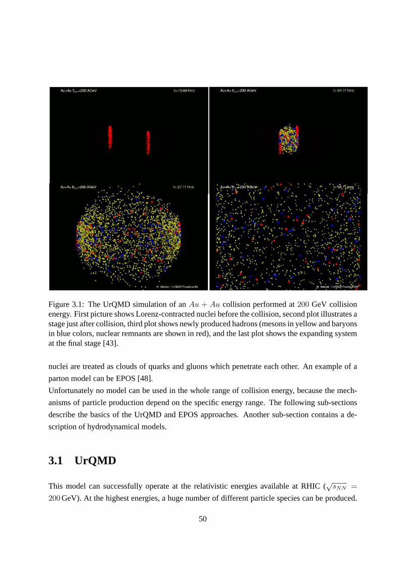
Figure 3.1: The UrQMD simulation of anAu + Au collision performed at200 GeV collisionenergy. First picture shows Lorenz-contracted nuclei before the collision, second plot illustrates astage just after collision, third plot shows newly producedhadrons (mesons in yellow and baryonsin blue colors, nuclear remnants are shown in red), and the last plot shows the expanding systemat the final stage [43].

nuclei are treated as clouds of quarks and gluons which penetrate each other. An example of a

parton model can be EPOS [48].

Unfortunately no model can be used in the whole range of collision energy, because the mech-

anisms of particle production depend on the specific energy range. The following sub-sections

describe the basics of the UrQMD and EPOS approaches. Another sub-section contains a de-

scription of hydrodynamical models.

3.1 UrQMD

This model can successfully operate at the relativistic energies available at RHIC (√

sNN =

200 GeV). At the highest energies, a huge number of different particle species can be produced.

50

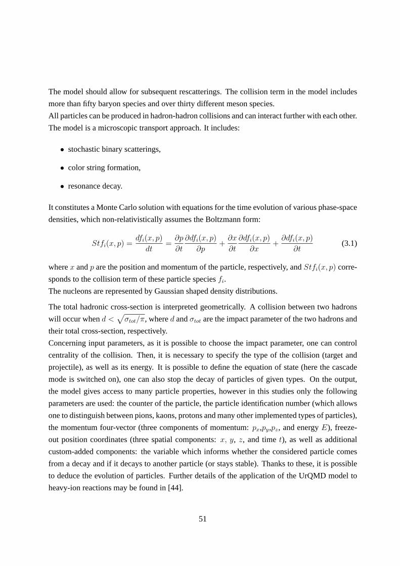
The model should allow for subsequent rescatterings. The collision term in the model includes

more than fifty baryon species and over thirty different meson species.

All particles can be produced in hadron-hadron collisions and can interact further with each other.

The model is a microscopic transport approach. It includes:

• stochastic binary scatterings,

• color string formation,

• resonance decay.

It constitutes a Monte Carlo solution with equations for the time evolution of various phase-space

densities, which non-relativistically assumes the Boltzmann form:

Stfi(x, p) =dfi(x, p)

dt=

∂p

∂t

∂dfi(x, p)

∂p+

∂x

∂t

∂dfi(x, p)

∂x+

∂dfi(x, p)

∂t(3.1)

wherex andp are the position and momentum of the particle, respectively, andStfi(x, p) corre-

sponds to the collision term of these particle speciesfi.

The nucleons are represented by Gaussian shaped density distributions.

The total hadronic cross-section is interpreted geometrically. A collision between two hadrons

will occur whend <√

σtot/π, whered andσtot are the impact parameter of the two hadrons and

their total cross-section, respectively.

Concerning input parameters, as it is possible to choose the impact parameter, one can control

centrality of the collision. Then, it is necessary to specify the type of the collision (target and

projectile), as well as its energy. It is possible to define the equation of state (here the cascade

mode is switched on), one can also stop the decay of particlesof given types. On the output,

the model gives access to many particle properties, howeverin this studies only the following

parameters are used: the counter of the particle, the particle identification number (which allows

one to distinguish between pions, kaons, protons and many other implemented types of particles),

the momentum four-vector (three components of momentum:px,py,pz, and energyE), freeze-

out position coordinates (three spatial components:x, y, z, and timet), as well as additional

custom-added components: the variable which informs whether the considered particle comes

from a decay and if it decays to another particle (or stays stable). Thanks to these, it is possible

to deduce the evolution of particles. Further details of theapplication of the UrQMD model to

heavy-ion reactions may be found in [44].

51

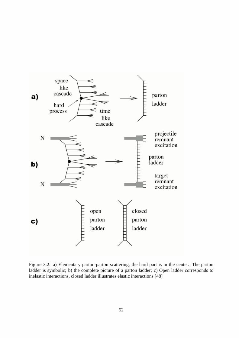
Figure 3.2: a) Elementary parton-parton scattering, the hard part is in the center. The partonladder is symbolic; b) the complete picture of a parton ladder; c) Open ladder corresponds toinelastic interactions, closed ladder illustrates elastic interactions [48]

52

Figure 3.3: Inner and outer contributions at various energies reached by experiments [48]

Figure 3.1 shows a short simulation of anAu+Au collision at200 GeV. Projectile nucleons: red

- target nucleons: red - mesons: yellow - excited baryons: blue.

The model reproduces the total, elastic and inelastic cross-sections of hadronic reactions. The

model predicts particle multiplicities (e.g. inclusive cross-sections) and (Lorenz invariant) cross

sections as well.

3.2 EPOS

The EPOS model is suited for a broad range of collision energies, it even takes into account

predictions for the LHC. In this model many reactions can be simulated, from simple nucleon-

nucleon collisions (such asp + p), through more complicated nucleon-nucleus systems (e.g.

d+Au) to the most complicated nucleus-nucleus collisions (e.g.Au+Au, Pb+Pb, Cu+Cu,...).

EPOS is an abbreviation, which stands for:

• Energy-conserving quantum mechanical multiple-scattering approach;

53

• Partons (parton ladders);

• Off-shell remnants;

• Splitting of parton ladders.

Produced partons are generally off-shell ones. They are represented by parton ladders. Each par-

ton ladder is translated into color strings, which fragmentinto hadrons. A parton ladder consist

of two parts: the hard one (discussed above) and the soft one (Figure 3.2, part 1). Two interact-

ing partons, one from the projectile and one from the target,leave remnants as a result of their

collision (Figure 3.2, part 2). A remnant can be interpretedas a di-quark with a string.

Open parton ladders correspond to inelastic scattering andclosed parton ladders illustrate elastic

scattering (Figure 3.2, part 3). There are two, highly significant nuclear “effects”: elastic (re-

lated to screening and saturation processes) and inelastic(bifurcation) splitting of parton ladders.

The idea of “energy-conserving multiple scattering” is simple: in the case of multiple scatter-

ing, when one has to calculate the partial cross-section fordouble, triple, .. scatterings, it is

necessary to take care about total energy which have to be shared among individual elementary

interactions. A consistent quantum-mechanical formulation requires the consideration of open

and closed parton ladders. The closed ladders do not contribute to particle production, but they

are significant since they affect the calculations of partial cross section. They lead to large num-

bers of interfering contributions for the same final state, all of which have to be summed up in

order to obtain the corresponding partial cross-section.

The contribution from partons is meant as ‘inner contribution’ and the one from remnants as

‘outer contributions’. In Figure 3.3, it is shown that remnants produce particles mainly in pe-

ripheral regions of rapidity and parton ladders- at centralrapidities. The inner contribution rises

with energy, and it dominates central rapidities at higher energies, whereas outer contributions

exist and have a stronger influence at lower energies, where inner contributions may not have

conditions to exist. At RHIC energies a significant remnant contribution still exist.

Concerning input parameters, it is necessary to chose the type and energy of the collision. If it

is required, it is also possible to stop decays of particles of some types. One can control central-

ity of the collision by choosing the impact parameter. The model gives access to many particle

properties. In these studies only the following characteristics are used: the index of the particle,

the particle identification number (which allows to distinguish between pions, kaons, protons

and many other implemented types of particles), momentum four-vector (three components of

momentum:px,py,pz, and energyE), freeze-out position coordinates (three spatial components:

54

x, y, z, and timet). Freeze-out coordinates were added to model specially fortwo-particle corre-

lations. Here also another additional components are used:the variable which informs whether

considered particle comes from a decay and if it decays to another particle (or stays stable). It is

thus possible to reproduce the particle history.

3.3 Hydrodynamics

If the system is macroscopic, then thermodynamics describes the static (temperature, pressure,

entropy, ...) and hydrodynamics- the dynamic (directed flow, anisotropic flow, particle produc-

tion versus transverse momentum, ...) properties of matter. In fact, the observed particle ratios

are close to the particle ratios in an ideal gas or fluid at the temperatureT ≃ 165MeV (while

lattice QCD predicts a phase transition at the temperatureT ≃ 175 MeV). This suggests that the

system evolves from a state close to the thermal equilibriumat the phase-transition boundary. On

the other hand, the thermal description reproduces hadron ratios inp + p ande+ + e− collisions,

where the system is small and the thermal equilibrium seems to be impossible. It is important to

point out here that as elementary collisions (suchp+p ande+ + e−) do not exhibit hydrodynam-

ical behavior, the excited systems produced as a result of such collisions are not macroscopic

ones. Therefore, a thermodynamic (static) description, not taking into account a hydrodynamic

(dynamic) one, can probe a macroscopic state. In contrast, experiments with heavy-ion collision

programs show evidence for hydrodynamic expansion, as momentum correlations are observed

in the energy domains, both SPS and RHIC.

Relativistic hydrodynamics is a set of conservation laws forthe energy-momentum tensorT µν

and the currentJµi in the case of fluid carrying conserved chargesNi.

∂µTµν = 0 (3.2)

and

∂µJµi = 0 (3.3)

In equilibrium,T µν andJµi are related to the properties of the fluid by the following relations:

T µν = (e + p)UµUν − pgµν (3.4)

and

Jµi = niU

µ (3.5)

55

Heree is energy density,p is pressure,ni is the number density of corresponding current,Uµ =

γ(1, υx, υy, υz) is the proper velocity of the fluid andJµi = niu

µ, whereNi =∑

i ni, g =

diag(+,−,−,−) is the metric tensor. In the case of strong interactions, theconserved currents

are: iso-spin(JµI ), strangeness(Jµ

S ), baryon number(JµB). For the hydrodynamical evolution,

iso-spin symmetry is assumed and the net strangeness is zerovalue, so only baryon current is

considered below.

The equations for the dynamics of an ideal fluid are specified by the ’Equation of State’ (EoS)

for the matter when the condition is setp = p(ǫ, n). Then, few elements can be specified: the

energyT 00 = E, the momentumT 0i = M i and the total chargeN0 = R. The equations of

motion:

∂tE + ∇ · (Ev) = −∇ · (pv) (3.6)

∂tM + ∇ · (Mv) = −∇p (3.7)

∂tM + ∇ · (Rv) = 0 (3.8)

Solving the EoS enables one to compare many experimental observables with hydrodynamical

predictions. Starting from single spectra distributions (calculated by hydrodynamics at given

temperature), through directed and anisotropic flow, dependence on impact parameter (trans-

formed often in heavy-ion collisions to the number of charged particles produced in such a

collision), momentum correlation: azimuthal and two-particle correlations and many other ob-

servables, help to better understand processes and reactions in collisions with a hydrodynamical

description. Recent results show that hydro successfully describes single-particle distributions,

and momentum spectra, reflects well particle productions versus their transverse momentum and

mass; however it fails in reproducing e.g HBT radii. More about hydrodynamical description of

heavy-ion collisions can be found in [49, 50].

56

Chapter 4

Two-particle correlations at small relative

velocities

Two-particle correlations at low relative velocities allow one to measure one of the smallest sizes

in nature, which corresponds to the size of a nucleon. They also make it possible to deduce

space-time properties of the sources. The measured sizes are of the order of10−15m (1 fm)

and therefore such two-particle correlation methods are called ‘femtoscopy’ [51]. The first such

measurement, which can be treated as an introduction to developing the two-particle interfer-

ometry method later, was performed in astronomy. R. Hanbury-Brown and R.Q. Twiss have

proposed a method (called HBT from their initials) [52] of estimating angular sizes of stellar

objects by studying the intensity of electromagnetic signals measured in coincidence. The inten-

sity interferometry for particles has similar origin, but uses particle momentum and is dedicated

to measuring space-time extent of the emitting source. Speaking more precisely, it is possible

to deduce the particle separation between sources emittingparticles using dependencies of their

relative momentum. Both the HBT method from astronomy and two-particle interferometry use

correlation techniques on one part of the phase space (whichcan be measured, e.g. photon in-

tensity in astronomy, particle momenta in nuclear collisions) to obtain information about a part

of phase space which is not measurable.

4.1 Identical non-interacting unpolarized nucleons and pions

Two identical particles with random polarization are emitted at the space-time pointsx1 and

x2, with four-momentap1 and p2 for the first and second particle, respectively (particles are

57

numbered due to a convention which has to be introduced). In asimpler picture of two spinless

bosons, the correlation function is determined by Quantum Statistics (QS) [53] (they are also

emitted at the space-time pointsx1 andx2 with their four-momentap1 andp2):

Rππ(p1, p2) =1

2

∣

∣ei(p1x1+p2x2) + ei(p1x2+p2x1)∣

∣

2(4.1)

The equation takes into account that it is impossible to exclude the scenario when the particle

with four-momentump1 is emitted from the space-time pointx2 and the particle with four-

momentump2 is emitted from the space-time pointx1. In the case of non-interacting identical

fermions with half spin values, the second factor is subtracted from the first one due to anti-

symmetrization of the wave function. In the case of nucleonsthere are two possible spin states:

S = 0 (singlet) andS = 1 (triplet), with populations of1/4 and3/4, respectively. The correlation

function is determined by QS.

Rnn(p1, p2) =1

4

[

1

2

∣

∣ei(p1x1+p2x2) + ei(p2x1+p1x2)∣

∣

2]

+3

4

[

1

2

∣

∣ei(p1x1+p2x2) − ei(p2x1+p1x2)∣

∣

2]

(4.2)

The first term corresponds to the singlet (spin-anti-symmetric) state and the second to triplet

(spin-symmetric) state. The correlation function (Equation 4.1) can be expressed in the form:

Rππ(p1, p2) = 1 + 〈cos(qx)〉 (4.3)

wherex ≡ t,−→x = x1 − x2 andq ≡ q0,−→q = p1 − p2. For Equation 4.2:

Rnn(p1, p2) =1

4[1 + 〈cos(qx)〉] +

3

4[1 − 〈cos(qx)〉] = 1 − 1

2〈cos(qx)〉 (4.4)

This results were obtained by Kopylov and Podgoretsky [54].In the case of a Gaussian space-

time distribution of emission points:

Si(xi) ∼ exp

[

−( −→xi√

2r0

)2

−(

ti√2τ0

)2]

(4.5)

wherer0 andτ0 are the source’s parameters respectively: size and time. Correlation functions

take then the form:

Rππ(p1, p2) = 1 + exp(−−→q2r2

0 − q20τ

20 ) (4.6)

Rnn(p1, p2) = 1 − 1

2exp(−

−→q2r2

0 − q20τ

20 ) (4.7)

58

for non-spin (e.g. identical pions) and spin dependencies (e.g. identical nucleons) respectively.

4.2 Identical non-interacting polarized nucleons

Nucleons (as the are baryons) interact through strong forces. In the case of populations of singlet

(ρ0) and triplet(ρ1) states dependent on the polarization vector,−→P following terms are consid-

ered: [55]

ρ0 =1

4(1 −

−→P 2

n) (4.8)

ρ1 =1

4(3 +

−→P 2

n) (4.9)

Then, the correlation function is given as:

Rnn(p1, p2) = 1 − 1 +−→P 2

n

2〈cos(qx)〉 (4.10)

4.3 Non-identical interacting nucleons (neutron - proton)

Below consideration may be applied to non-identical systemslike proton - anti-proton but there

Coulomb interactions has to be taken into account additionally.

Due to interaction between particles, the plane-wave in theprevious example is replaced by the

Bethe-Salpeter amplitude [56]:

ei(p1x1+p2x2) → ψ(S)p1p2

(x1, x2) = ei(p1x1+p2x2) + ϕ(S)p1p2

(x1, x2) (4.11)

whereϕ(S)p1p2(x1, x2) is the scattered wave. In this case, the correlation function takes the form:

Rnp(p1, p2) = ρ0

⟨∣

∣ψ(0)p1p2

(x)∣

∣

⟩2+ ρ1

⟨∣

∣ψ(1)p1p2

(x)∣

∣

⟩2(4.12)

Hereψ(S)p1p2(x) is obtained from the Bethe-Salpeter amplitude after separation of the c.m.s motion:

ψ(S)p1p2

(x1, x2) = eiPXψ(S)p1p2

(x) (4.13)

whereP = p1 + p2, X = [(p1P )x1 + (p2P )x2]/P2 = X0,

−→R is the two-particle c.m.s four-

coordinate.

59

The populations of singlet and triplet states are:

ρ0 =1

4(1 −−→

Pn−→Pp) (4.14)

ρ1 =1

4(3 +

−→Pn

−→Pp) (4.15)

Now, x∗ = (−→r∗ , t∗) in the c.m.s of the pair is defined. The amplitudeψ

(S)p1p2(x1, x2) is replaced

by the wave functionψ(S)(+)

−

−→k∗

(−→r∗) describing the relative motion of particles with asymptotic

(r∗ → ∞) of a superposition of the plane and diverging spherical wave:

ψ(S)(+)

−

−→k∗

(−→r∗) → ei

−→k∗−→r∗ + f (S)(

−→k∗)

ei−→k∗−→r∗

r∗(4.16)

wherek∗ =√

−q2/2.

4.4 Identical interacting particles

Replacing the plane waves with Bethe-Salpeter amplitudes, the formula is:

Rnn(p1, p2) =1

4(1−

−→P 2

n)

⟨

∣

∣

∣

∣

1√2

(

ψ(0)p1p2

(x) + ψ(0)p2p1

(x))

∣

∣

∣

∣

2⟩

+1

4(3+

−→P 2

n)

⟨

∣

∣

∣

∣

1√2

(

ψ(0)p1p2

(x) + ψ(0)p2p1

(x))

∣

∣

∣

∣

2⟩

(4.17)

4.5 Deuteron formation rate

Assuming that deuteron formation is dominated by the FSI between emitted protons and neutron,

it is possible to form a deuteron state. The cross-section for a creation of such a system is given

by the formula:

σ(1)d (Pd) = (2π)3γρ1

⟨

∣

∣

∣ψ

(1)b (x)

∣

∣

∣

2⟩

σnp(1

2Pd,

1

2Pd) (4.18)

whereγ is the Lorenz factor,ψ(1)b (x) is the Bethe-Salpeter amplitude describing the bound triplet

state of neutron and proton.σnp(12Pd,

12Pd) ≃ σnp(p1, p2) is the production cross-section of un-

correlated(n, p) pairs. It is related to the measured(n, p) production cross-sectionσnp(p1, p2)

60

through the correlation function:

σnp(p1, p2) = Rnp(p1, p2)σnp(p1, p2) (4.19)

The deuteron formation cross-section is related to the emission is(p, n) pairs with nearby mo-

menta.

4.6 The treatment of Coulomb Interaction

In the case of charged particles, long-range Coulomb FSI are observed. The pair wave function

is described then:

Ψ(S)−→k∗

(−→r∗) =√

A±

C exp(iδC0 )F (−iη, 1, iξ) (4.20)

whereAC is the Gamow factor.

A±

C (k∗) = ± (2π/k∗aC)1

exp [± (2π/k∗aC)] − 1(4.21)

the sign+(−) corresponds to repulsion (attraction),k∗ is the momentum of one particle in the

PRF (Pair Rest Frame reference),aC =2( h

2π )2

me2 is the Bohr radius for particles with unit charges

(for protonsaC = 57.5fm), δCo = arg Γ (1 + i/k∗aC) is the Coulomb s-wave phase shift,

F (−iη, 1, iξ) is the confluent hypergeometrical function whereη = 1/(k∗ac), ξ = qr∗ +−→q −→r∗ =

qr∗(1 + cosθ∗) andθ∗ is the angle between particle relative momentum−→q and the initial separa-

tion−→r∗ .

4.7 Combining Strong and Coulomb interaction

Systems which requires combining both of FSI are first of all combinations of baryons (strong

interactions dominate in baryon systems in smaller sources), then combinations of two mesons

and mesons with baryons. The Coulomb interaction is a modification of the wave-function of the

pair and of both incoming plane waves, including the scattered wave. The scattering amplitude

becomes then:

f(−→k∗) =

[

1

f0

+1

2d0k

∗2 − 2

ac

h(k∗ac) − ik∗Ac(k∗)

]−1

(4.22)

61

In the case of proton-proton interactionf0 = 7.77fm andd0 = 2.77fm. The functionh(x) has

the following form:

h(x) =1

x2

∞∑

n=1

1

n(n2 + x−2)− C + ln|x| (4.23)

whereC is constant.

4.8 Parametrization of correlation function of identical pions

Very often, the source is assumed to be a three-dimensional sphere described by a Gaussian

density distribution in space-time. The−→q vector can be decomposed into three components, the

parametrization of the correlation function was proposed by Kopylov and Podgoretsky [57] (K-

P parametrization) and by Bertsch-Pratt (Bertsch-Pratt decompositions) [58] (Figure 4.1). The

longitudinal componentqlong is parallel to the beam axis (the z-axis), the outward component

qout is parallel to the transverse momentum of the pair (−→KT ) and the sideward componentqside

is perpendicular to both of them. More details can be found inthe caption of the figure. In this

case, one can obtain the following parametrization of the correlation function1 determined by

QS (it is assumed that the cross-terms vanish due to symmetryreasons):

C(qout, qside, qlong, λ) = 1 + λexp(

−q2outr

2out − q2

sider2side − q2

longr2long

)

(4.24)

whererout, rside andrlong are the size of the source in theout, side andlong direction, respec-

tively; the λ parameter indicates the strength of the correlation and is anumber in the range

[0.0, 1.0]. Values ofλ lower than1.0 are observed experimentally and are attributed to several

reasons: the admixture of misidentified particles, the inclusion of non-correlated pairs and detec-

tor inefficiencies. Frequently, the correlation function is also analyzed as a function of only one

variable - the value of relative momentum in the pair rest frame,Qinv:

C(Qinv; r0, λ) = 1 + λexp(

−Q2invr

20

)

(4.25)

The correlation function fitted by one of above formulas provides the source size - the Gaussian

radius of the sourcer0 in the case of 1-dimensional correlation functions, or three radii: rout,

rside, rlong in the case of 3-dimensional correlation functions.

Very often the correlation function is measured for particles which interact by Coulomb and/or

1The correlation function is denoted byC, however very often different notations are used as well:CF , R

62

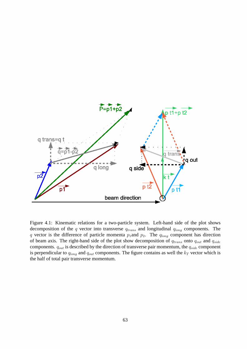
Figure 4.1: Kinematic relations for a two-particle system.Left-hand side of the plot showsdecomposition of theq vector into transverseqtrans and longitudinalqlong components. Theq vector is the difference of particle momentap1and p2. The qlong component has directionof beam axis. The right-hand side of the plot show decomposition of qtrans onto qout andqside

components.qout is described by the direction of transverse pair momentum, theqside componentis perpendicular toqlong andqout components. The figure contains as well thekT vector which isthe half of total pair transverse momentum.

63

strong forces. Such interactions have to be taken into account when trying to deduce the source

size.

4.9 Theoretical predictions forπ − π, p− p and p− p systems

The top panel of Figure 4.2 shows theoretical predictions for π+π+ system for a number of

source sizes:3fm, 5fm, 10fm and20fm. Only sources withλ = 1 are considered (λ = 1 is

assumed). For each source size complete calculations including QS and Final State Interactions

(FSI) [59, 60] have been performed. The figure also contains calculations for the QS effect only

(3 and20 fm). In this case, the correlation function reaches the value of2.0 for Qinv = 0 GeV/c.

In the case of a bigger source (20fm), the correlation effect decreases faster. (The finite size

of bins causes the first point of correlation does not reach2.0). For smallQinv, the correlation

function goes to zero due to Coulomb repulsion. The strength of correlation increases with de-

creasing source-size.

The bottom panel of Figure 4.2 shows theoretical predictions for the (p−p) system. Calculations

for many source sizes are presented. The correlation effectfor the case of identical fermions

such asp− p andp− p is driven by anti-symmetrization of the wave function determined by QS.

Two FSI exist in this system as well: protons are repelled by Coulomb forces and they strongly

interact. For smaller sources, the correlation has a peak for Qinv = 40 MeV due to interplay

of all types of correlation effects. Coulomb FSI repulsion causes that the correlation function

for Qinv → 0GeV/c. The correlation strength depends directly on the source size, it decreases

with increasing the source size. In Figure 4.3, theoreticalpredictions for proton-proton (p − p)

and proton- anti-proton (p − p) correlations are shown. The second part of the plot is dedicated

to p − p interactions. Proton - anti-proton combinations have not been measured so far due to

not sufficient statistic. However, the description of the strong interaction between proton and its

anti-particle has not been estimated with a high accuracy. Theorists needed experimental mea-

surements in order to improve the scattering calculations for such system. Inp − p correlations,

only FSI occur. Here the characteristic, wide band below unity corresponding to annihilation

processes between particles and their anti-particles appears. Even if, the assumedp−p andp−p

source sizes are the same (here3fm), it does not lead to the same range of interactions: thep− p

correlation can be twice as wide as forp− p. Depending on the source size, the correlation func-

tion can have a different shape, as strong interactions are more dominant on smaller distances.

These two simulations were prepared assuming Gaussian source distributions with the radius of

64

Figure 4.2: Top panel: pion - pion correlation functions forassumed source sizes:3 fm includingQS only (black stars) and for QS and FSI (bright blue points);5 fm QS + FSI (green triangles);10 fm for complete calculations (blue squares);20 fm for QS only (pink open circles) and for QS+ FSI (black circles). Bottom panel: proton - proton correlation functions for 6 different sourcesizes: 2 fm (dark blue squares),3fm (green triangles),5fm (red triangles),10fm (gray closedcircles),20fm (black open circles) and50 fm (pink open squares) [61].

65

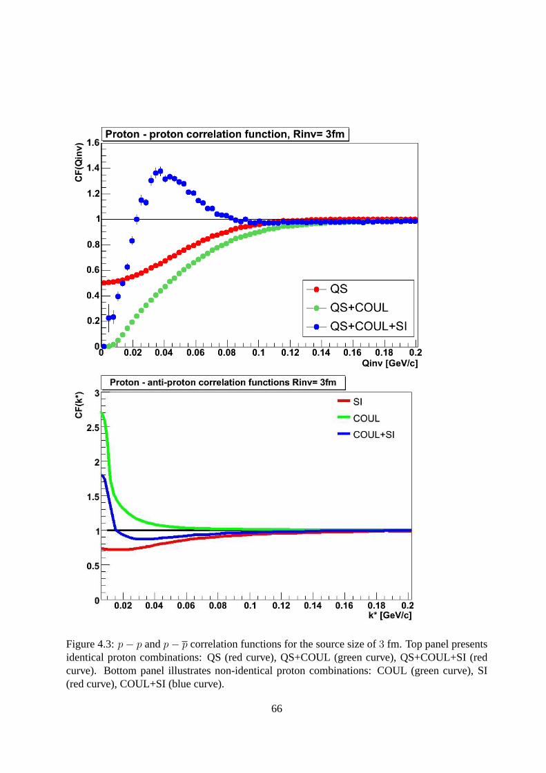
Figure 4.3:p − p andp − p correlation functions for the source size of3 fm. Top panel presentsidentical proton combinations: QS (red curve), QS+COUL (green curve), QS+COUL+SI (redcurve). Bottom panel illustrates non-identical proton combinations: COUL (green curve), SI(red curve), COUL+SI (blue curve).

66

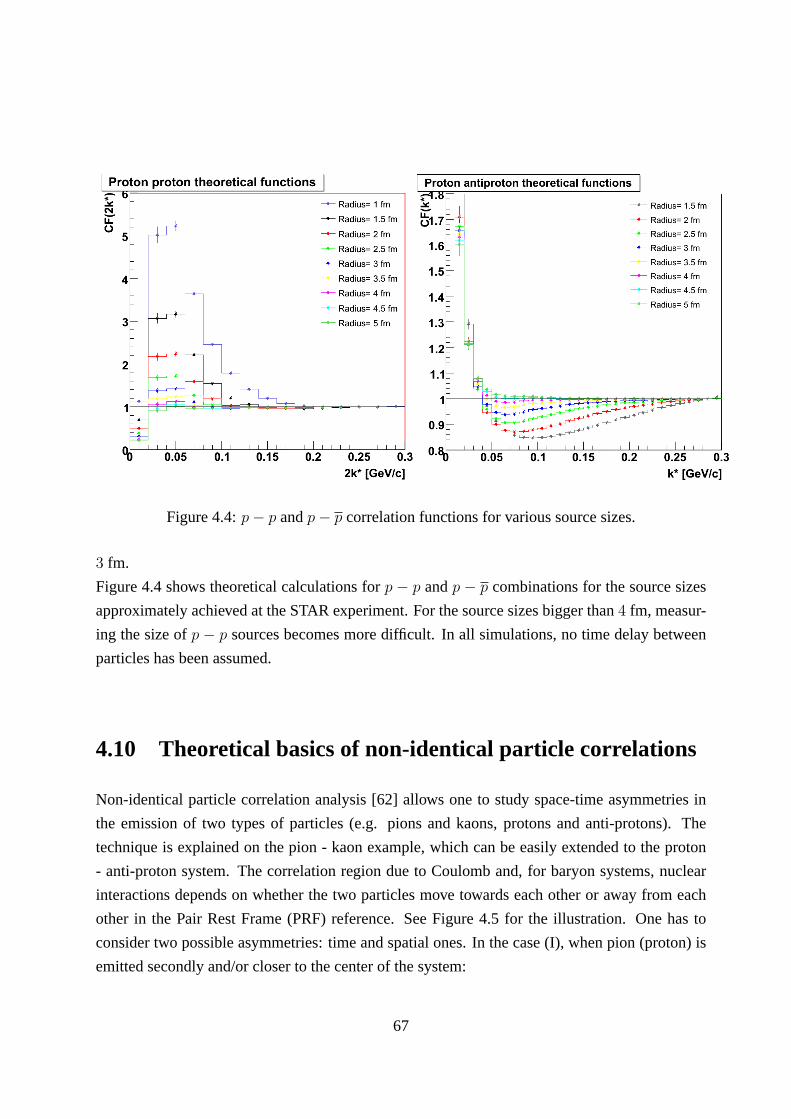
Figure 4.4:p − p andp − p correlation functions for various source sizes.

3 fm.

Figure 4.4 shows theoretical calculations forp − p andp − p combinations for the source sizes

approximately achieved at the STAR experiment. For the source sizes bigger than4 fm, measur-

ing the size ofp − p sources becomes more difficult. In all simulations, no time delay between

particles has been assumed.

4.10 Theoretical basics of non-identical particle correlations

Non-identical particle correlation analysis [62] allows one to study space-time asymmetries in

the emission of two types of particles (e.g. pions and kaons,protons and anti-protons). The

technique is explained on the pion - kaon example, which can be easily extended to the proton

- anti-proton system. The correlation region due to Coulomb and, for baryon systems, nuclear

interactions depends on whether the two particles move towards each other or away from each

other in the Pair Rest Frame (PRF) reference. See Figure 4.5 forthe illustration. One has to

consider two possible asymmetries: time and spatial ones. In the case (I), when pion (proton) is

emitted secondly and/or closer to the center of the system:

67

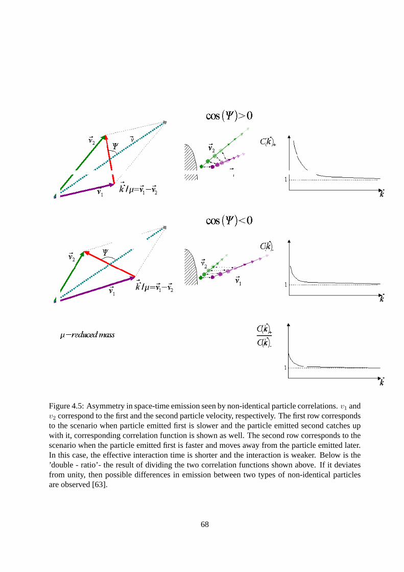
Figure 4.5: Asymmetry in space-time emission seen by non-identical particle correlations.v1 andv2 correspond to the first and the second particle velocity, respectively. The first row correspondsto the scenario when particle emitted first is slower and the particle emitted second catches upwith it, corresponding correlation function is shown as well. The second row corresponds to thescenario when the particle emitted first is faster and moves away from the particle emitted later.In this case, the effective interaction time is shorter and the interaction is weaker. Below is the’double - ratio’- the result of dividing the two correlationfunctions shown above. If it deviatesfrom unity, then possible differences in emission between two types of non-identical particlesare observed [63].

68

• Time asymmetry (particles are assumed to be emitted from thesame positions); the kaon

(anti-proton) is considered as emitted first, the pion (proton) second

• Spatial asymmetry (particles are assumed to be emitted at the same time); the pion (proton)

is assumed to be emitted closer to the center of system and kaon (anti-proton) is considered

as emitted further from the system center

– A) the pion (proton) is faster than the kaon (anti-proton); the pion (proton) catches

up with the kaon (anti-proton)

– B) the pion (proton) is slower than the kaon (anti-proton); the kaon (anti-proton)

moves away

In both A cases the correlation effect is stronger and the duration of interaction is longer than in

B cases. Such stronger correlation functions are marked byC+(k∗

out), and the weaker ones by

C−(k∗

out).

It is also possible to consider the opposite scenario, case (II): the pion (proton) is emitted first

and/or closer to the edge of the system:

• Time asymmetry (particles are assumed to be emitted from thesame positions); the pion

(proton) is considered as emitted first, the kaon (anti-proton) second

• Spatial asymmetry (particles are assumed to be emitted at the same time); the pion (pro-

ton) is assumed to be emitted closer to the edge of the system and the kaon (anti-proton) is

considered as emitted further to the edge of the system

– A) the kaon (anti-proton) is faster than the pion (proton); the kaon (anti-proton)

catches up with the pion (proton)

69

– B) the kaon (anti-proton) is slower than the pion (proton); the pion (proton) moves

away

Again, in both A cases the correlation effect is stronger andthe duration of interaction is longer

than in B cases. Such stronger correlation functions are marked byC+(k∗

out), and the weaker

ones byC−(k∗

out).

In our analysis the convention (I) is assumed; fork∗

out > 0, the pion (proton) is faster and for

k∗

out < 0 the pion (proton) is slower. By studying the ratio of functions for positive and negative

values ofk∗

out < 0, the information about space-time asymmetry is deduced as adeviation from

unity. One can study asymmetries in different directions byanalyzing the correlations dependent

on negative and positive components ofk∗ projections in three directions: theout, side, and

long components. In STAR, due to azimuthal symmetry and symmetry at midrapidity, the mean

differences:< r∗side >=< r∗long >= 0. The asymmetry can be seen for theout projection and it

is a mixture of two components:< r∗out >=< rout > −βt < t >[64].

4.11 The experimental approach

In the experimental case, the correlation function is defined as a ratio of the probability of regis-

tering two particles simultaneously (in the same event) to the product of registering probabilities

of such particles independently (in different events). It can be therefore obtained by dividing

two-particle distribution by two single-particle distributions:

C(p1, p2) =P (p1, p2)

P (p1)P (p2)(4.26)

This formula can be also expressed in the formalism of cross-sections:

C(p1, p2) ∝(

d6σ

d3p1d3p2

)

Á

(

d3σ

d3p1

d3σ

d3p2

)

(4.27)

Usually, the correlation function is analyzed as a functionof pair relative momentum−→q , consid-

ered in the frame, the pair’s center-of-mass is at the rest, the Pair Rest Frame (PRF).

Constructing the correlation function in the experiment, one has put pairs of particles coming

from the same event into numerator (particles are correlated) and pairs of particles from different

70

events (non-correlated, as a the reference):

C(p1, p2) =A(p1, p2)

B(p1, p2)(4.28)

4.12 An experimental review of identical and non-identical

particle correlations

Below is a short experimental review of the most significant results concerning identical particle

correlations: excitation functions showing source-size dependencies for various values of colli-

sion energy, centrality dependencies versus transverse mass of pion source sizes and multiplicity

scaling of radii.

Excitation function

Figure 4.6 shows HBT parameters (source sizes:Rout,Rside, Rlong andλ parameter) vs. collision

energy for midrapidity. The data for centralAu+Au, Pb+Pb andPb+Au collisions describes

π−π− correlations at low transverse momenta. The large source sizes and/or lifitimes were sug-

gested as potential signatures of the QGP state formation. An increase of∼ 10% (but not more)

in the transverse radiiRo andRs is observed. In the case ofRs, the increase might correspond

to the large freeze-out volume for a larger pion multiplicity. Rl is slightly increasing for higher

energies. The increase predicted by hydrodynamics in the ratio of Ro/Rs as a probe of QGP

formation, is not observed.Ro/Rs is correlated with the emission duration. Hydrodynamical

models typically calculate this value approximately equalto 1.5 and moderately dependent on

kT range. TheRo/Rs versus collision energy reflects flat dependence and is equalapproximately

to the unity, what indicates shorter than predicted by hydrodynamics emission duration. The dif-

ferences between radii for√

sNN = 200 GeV (open and closed symbols) occur due to different

methods of Coulomb correction [66, 67] applied in these two analysis, respectively. Smallerλ

parameter,Ro andRs values can be explained by applying different criteria in particle selections.

This plot illustrates that the collision energy is not a scaling variable for HBT radii. Such be-

havior is known asHBT puzzle. As it was expected- for higher energies there should occur an

increase of the radii (forout component specially), however the excitation function presents that

the region showing this signature of the phase transition has not been achieved yet.

71

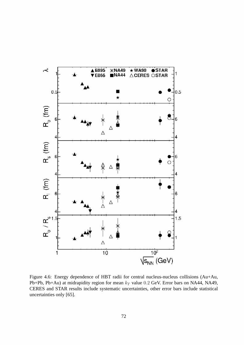
Figure 4.6: Energy dependence of HBT radii for central nucleus-nucleus collisions (Au+Au,Pb+Pb, Pb+Au) at midrapidity region for meankT value0.2 GeV. Error bars on NA44, NA49,CERES and STAR results include systematic uncertainties, other error bars include statisticaluncertainties only [65].

72

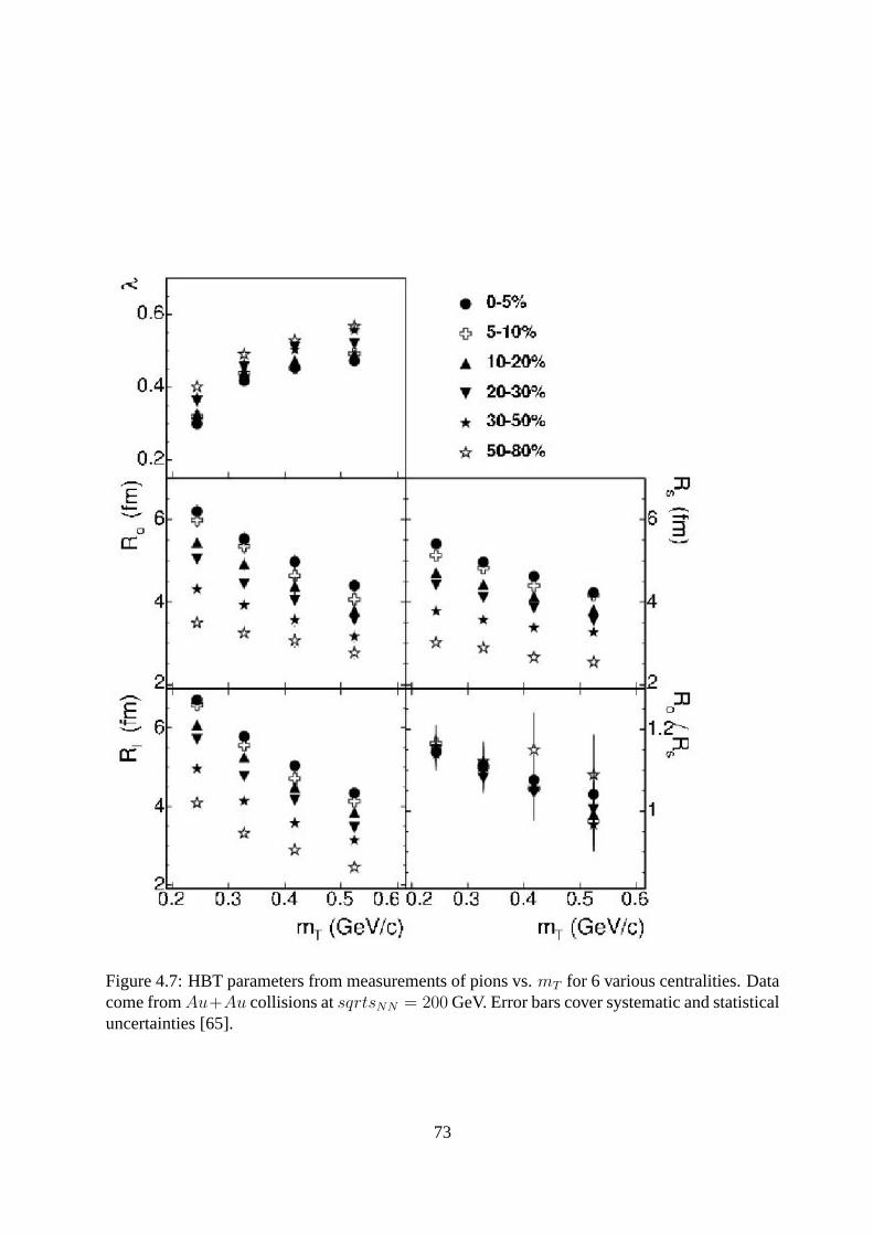
Figure 4.7: HBT parameters from measurements of pions vs.mT for 6 various centralities. Datacome fromAu+Au collisions atsqrtsNN = 200 GeV. Error bars cover systematic and statisticaluncertainties [65].

73

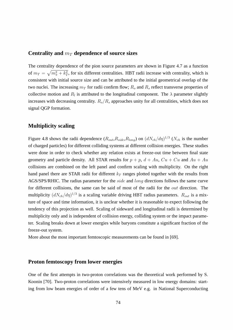
Centrality and mT dependence of source sizes

The centrality dependence of the pion source parameters areshown in Figure 4.7 as a function

of mT =√

m2π + k2

T , for six different centralities. HBT radii increase with centrality, which is

consistent with initial source size and can be attributed tothe initial geometrical overlap of the

two nuclei. The increasingmT for radii confirm flow;Ro andRs reflect transverse properties of

collective motion andRl is attributed to the longitudinal component. Theλ parameter slightly

increases with decreasing centrality.Ro/Rs approaches unity for all centralities, which does not

signal QGP formation.

Multiplicity scaling

Figure 4.8 shows the radii dependence (Rout,Rside,Rlong) on (dNch/dη)1/3 (Nch is the number

of charged particles) for different colliding systems at different collision energies. These studies

were done in order to check whether any relation exists at freeze-out time between final state

geometry and particle density. All STAR results forp + p, d + Au, Cu + Cu andAu + Au

collisions are combined on the left panel and confirm scalingwith multiplicity. On the right

hand panel there are STAR radii for differentkT ranges plotted together with the results from

AGS/SPS/RHIC. The radius parameter for theside andlong directions follows the same curve

for different collisions, the same can be said of most of the radii for the out direction. The

multiplicity (dNch/dη)1/3 is a scaling variable driving HBT radius parameters.Rout is a mix-

ture of space and time information, it is unclear whether it is reasonable to expect following the

tendency of this projection as well. Scaling of sideward andlongitudinal radii is determined by

multiplicity only and is independent of collision energy, colliding system or the impact parame-

ter. Scaling breaks down at lower energies while baryons constitute a significant fraction of the

freeze-out system.

More about the most important femtoscopic measurements canbe found in [69].

Proton femtoscopy from lower energies

One of the first attempts in two-proton correlations was the theoretical work performed by S.

Koonin [70]. Two-proton correlations were intensively measured in low energy domains: start-

ing from low beam energies of order of a few tens of MeV e.g. in National Superconducting

74

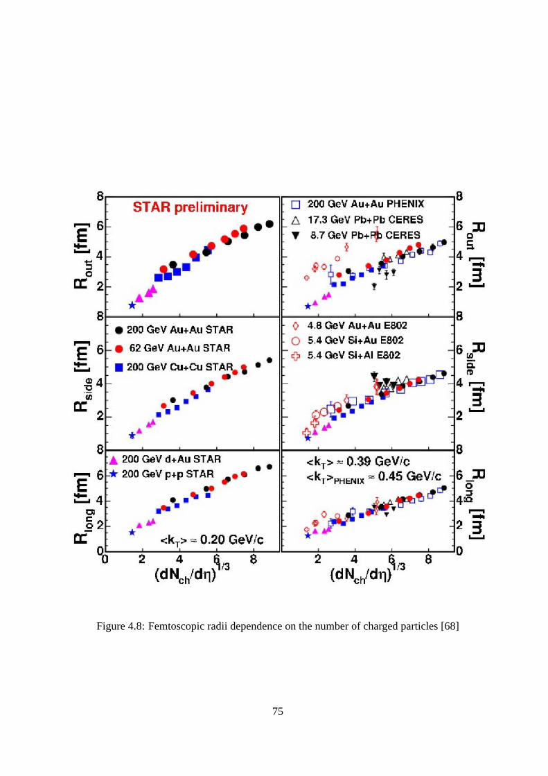
Figure 4.8: Femtoscopic radii dependence on the number of charged particles [68]

75

Figure 4.9: The influence of different experimental factorson the form of the measured correla-tion function. The example is for a Gaussian source withr0 = 2.38 fm., where each effect hasbeen added cumulatively [75].

76

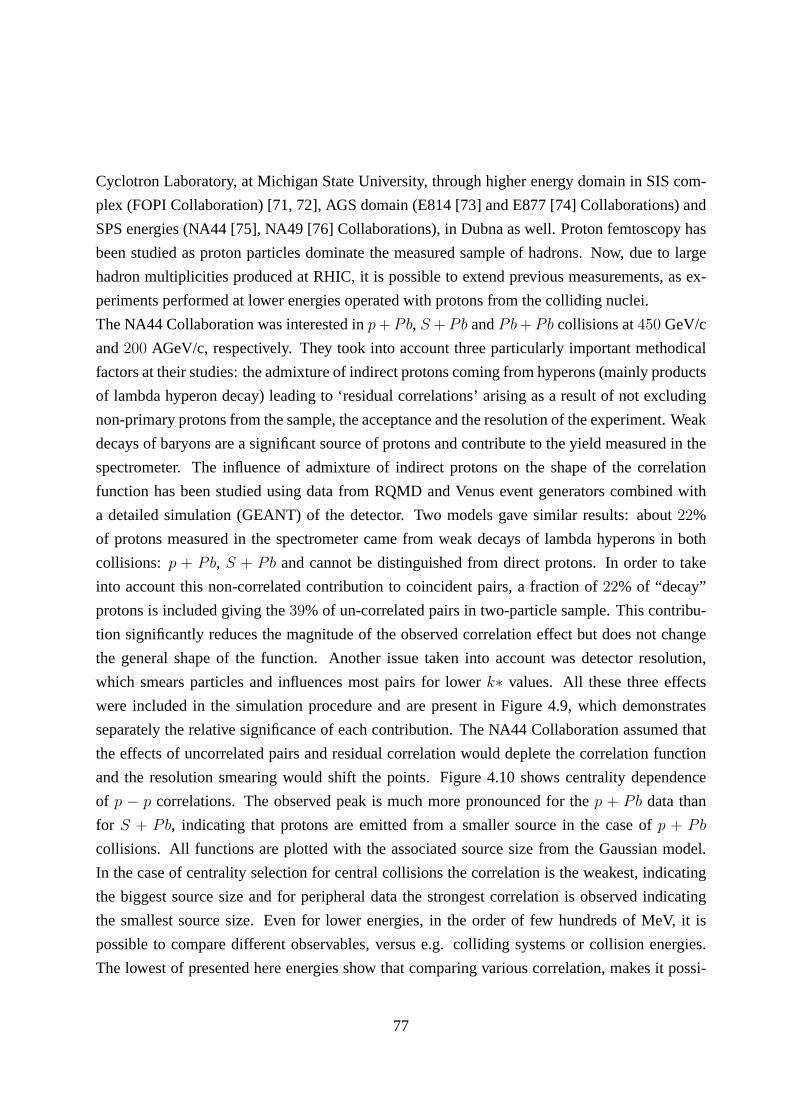
Cyclotron Laboratory, at Michigan State University, through higher energy domain in SIS com-

plex (FOPI Collaboration) [71, 72], AGS domain (E814 [73] andE877 [74] Collaborations) and

SPS energies (NA44 [75], NA49 [76] Collaborations), in Dubnaas well. Proton femtoscopy has

been studied as proton particles dominate the measured sample of hadrons. Now, due to large

hadron multiplicities produced at RHIC, it is possible to extend previous measurements, as ex-

periments performed at lower energies operated with protons from the colliding nuclei.

The NA44 Collaboration was interested inp + Pb, S + Pb andPb + Pb collisions at450 GeV/c

and200 AGeV/c, respectively. They took into account three particularly important methodical

factors at their studies: the admixture of indirect protonscoming from hyperons (mainly products

of lambda hyperon decay) leading to ‘residual correlations’ arising as a result of not excluding

non-primary protons from the sample, the acceptance and theresolution of the experiment. Weak

decays of baryons are a significant source of protons and contribute to the yield measured in the

spectrometer. The influence of admixture of indirect protons on the shape of the correlation

function has been studied using data from RQMD and Venus eventgenerators combined with

a detailed simulation (GEANT) of the detector. Two models gave similar results: about22%

of protons measured in the spectrometer came from weak decays of lambda hyperons in both

collisions: p + Pb, S + Pb and cannot be distinguished from direct protons. In order totake

into account this non-correlated contribution to coincident pairs, a fraction of22% of “decay”

protons is included giving the39% of un-correlated pairs in two-particle sample. This contribu-

tion significantly reduces the magnitude of the observed correlation effect but does not change

the general shape of the function. Another issue taken into account was detector resolution,

which smears particles and influences most pairs for lowerk∗ values. All these three effects

were included in the simulation procedure and are present inFigure 4.9, which demonstrates

separately the relative significance of each contribution.The NA44 Collaboration assumed that

the effects of uncorrelated pairs and residual correlationwould deplete the correlation function

and the resolution smearing would shift the points. Figure 4.10 shows centrality dependence

of p − p correlations. The observed peak is much more pronounced forthe p + Pb data than

for S + Pb, indicating that protons are emitted from a smaller source in the case ofp + Pb

collisions. All functions are plotted with the associated source size from the Gaussian model.

In the case of centrality selection for central collisions the correlation is the weakest, indicating

the biggest source size and for peripheral data the strongest correlation is observed indicating

the smallest source size. Even for lower energies, in the order of few hundreds of MeV, it is

possible to compare different observables, versus e.g. colliding systems or collision energies.

The lowest of presented here energies show that comparing various correlation, makes it possi-

77

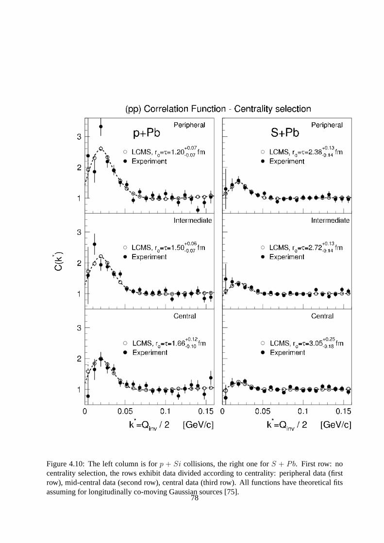
Figure 4.10: The left column is forp + Si collisions, the right one forS + Pb. First row: nocentrality selection, the rows exhibit data divided according to centrality: peripheral data (firstrow), mid-central data (second row), central data (third row). All functions have theoretical fitsassuming for longitudinally co-moving Gaussian sources [75].

78

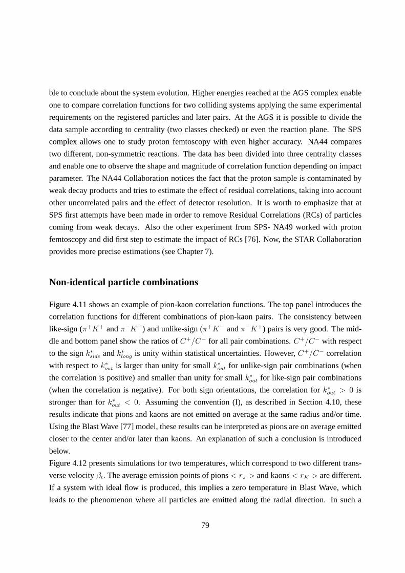
ble to conclude about the system evolution. Higher energiesreached at the AGS complex enable

one to compare correlation functions for two colliding systems applying the same experimental

requirements on the registered particles and later pairs. At the AGS it is possible to divide the

data sample according to centrality (two classes checked) or even the reaction plane. The SPS

complex allows one to study proton femtoscopy with even higher accuracy. NA44 compares

two different, non-symmetric reactions. The data has been divided into three centrality classes

and enable one to observe the shape and magnitude of correlation function depending on impact

parameter. The NA44 Collaboration notices the fact that the proton sample is contaminated by

weak decay products and tries to estimate the effect of residual correlations, taking into account

other uncorrelated pairs and the effect of detector resolution. It is worth to emphasize that at

SPS first attempts have been made in order to remove Residual Correlations (RCs) of particles

coming from weak decays. Also the other experiment from SPS-NA49 worked with proton

femtoscopy and did first step to estimate the impact of RCs [76].Now, the STAR Collaboration

provides more precise estimations (see Chapter 7).

Non-identical particle combinations

Figure 4.11 shows an example of pion-kaon correlation functions. The top panel introduces the

correlation functions for different combinations of pion-kaon pairs. The consistency between

like-sign (π+K+ andπ−K−) and unlike-sign (π+K− andπ−K+) pairs is very good. The mid-

dle and bottom panel show the ratios ofC+/C− for all pair combinations.C+/C− with respect

to the signk∗

side andk∗

long is unity within statistical uncertainties. However,C+/C− correlation

with respect tok∗

out is larger than unity for smallk∗

out for unlike-sign pair combinations (when

the correlation is positive) and smaller than unity for small k∗

out for like-sign pair combinations

(when the correlation is negative). For both sign orientations, the correlation fork∗

out > 0 is

stronger than fork∗

out < 0. Assuming the convention (I), as described in Section 4.10,these

results indicate that pions and kaons are not emitted on average at the same radius and/or time.

Using the Blast Wave [77] model, these results can be interpreted as pions are on average emitted

closer to the center and/or later than kaons. An explanationof such a conclusion is introduced

below.

Figure 4.12 presents simulations for two temperatures, which correspond to two different trans-

verse velocityβt. The average emission points of pions< rπ > and kaons< rK > are different.

If a system with ideal flow is produced, this implies a zero temperature in Blast Wave, which

leads to the phenomenon where all particles are emitted along the radial direction. In such a

79

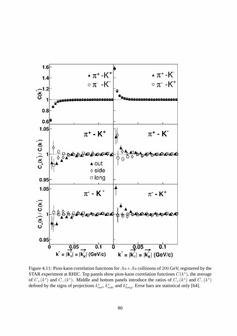
Figure 4.11: Pion-kaon correlation functions forAu+Au collisions of200 GeV, registered by theSTAR experiment at RHIC. Top panels show pion-kaon correlation functionsC(k∗), the averageof C+(k∗) andC−(k∗). Middle and bottom panels introduce the ratios ofC+(k∗) andC−(k∗)defined by the signs of projectionsk∗

out, k∗

side andk∗

long. Error bars are statistical only [64].

80

Figure 4.12: Distributions of emission points in the transverse plane, for different particle speciesat the same velocity. Top panels introduce pions, middle one- kaons, bottom ones- protons. Leftpanels show simulations where velocity is assumed toβt = 0.907 and right panels correspond tothe estimation ofβt = 0.974. Dashed curves show Blast-wave predictions [77].

81

profile, all particles are emitted from the same space-time point, independly on their mass. How-

ever, in Blast Wave, a particle velocity is sum of the flow velocity βf (which does not depend on

mass; it is determined by the flow field and a thermal velocityβt. In the case of non-identical

particles (with different masses) particles with the sameβf andβt, thus identical momenta are

produced, but their velocities are not identical. For particles with smaller masses, the averageβt

is relatively larger, indicating the spread of the emissionpoint is larger for lighter particles (here,

pions). This is the reason why the average emission point of pions is closer to the center that in

the case of kaons. This effect is also dependent on temperature, as higher temperature provides

stronger flow. This leads to the conclusion that on average, pions and kaons are emitted from

different areas.

4.13 Baryonic systems

Strong flow occurring inAu + Au collisions at√

sNN = 200 GeV causes that from correlations

smaller sizes of emitting areas at given temperature are given. The results on baryon femtoscopy

comply with the ones from meson interferometry and confirm such a hypothesis of flow.

On one hand, thep − Λ andp − Λ interaction potentials are relatively well known; on the other

p−Λ andp−Λ interaction potentials have been estimated by the STAR Collaboration for the first

time. Constraining baryon - anti-baryon potentials, the information determinesp − Λ andp − Λ

annihilation cross sections. Figure 4.13 presents combined p−Λ ⊕ p−Λ andp−Λ ⊕ p−Λ cor-

relation functions. The symbol⊕ means that the numerators and denominators of the systems

have been added to build a combine correlation function. In both functions, the curves corre-

spond to the fit carried out using the Lednicky - Lyuboshits formalism [78]. The radii extracted

from like-sign (r0 = 3.09±0.34+0.17−0.25±0.2fm) and unlike-sign (r0 = 1.50±0.05+0.10

−0.12±0.3fm)

[79] correlations are significantly different. The error bars include both statistical and systematic

uncertainties. This difference was unexpected. Correlation functions shown here are corrected

with the best estimate of purity, however not taking into account any RCs. Their effect to strange

baryon combinations is expected to be significant (more about estimating the residual correla-

tions in proton and anti-proton femtoscopy in Section 6). Inthe case of poor knowledge of

strong interactions between two particles in such exotic systems as (M=meson)MΛ andΛΛ the

correlation measurement of scattering lengths might be highly useful. In heavy-ion collisions,

the effective radiusr0 of the emission region should be considered much larger thanthe range

of strong interaction potential. At smallk∗ the FSI contribution to the correlation function is

determined by s-wave scattering amplitudef s(k∗). In the case of|f s| > r0, the contribution is

82

Figure 4.13: Top panel:p−Λ⊕ p−Λ andp−Λ⊕ p−Λ correlation functions corrected for purityand momentum resolution. Curves corresponds to fits done using the Lednicky & Lyuboshitzanalytical model [79]; bottom panel illustrates the correlation function forΛΛ system for fewsource-sizes.

83

of the order of|f0/r0|2 and dominates the effect of QS (in identical particle correlation), in the

opposite case the sensitivity of the correlation function to the scattering amplitude is determined

by the linear expressionf s/r0. Theoretical predictions of theΛΛ system are presented in Figure

4.13.

Chapter 5 describes experimental complexes of RHIC accelerator, Chapter 6 contains a detailed

description of the whole data analysis and encloses complexresults concerning proton fem-

toscopy. and Chapter 7 contains results for proton femtoscopy performed at RHIC.

84

Chapter 5

The STAR experiment

In this chapter the STAR experiment is presented. During seven years of operation, STAR has

collected an impressive amount of data, which is used to calculate two-proton femtoscopy pre-

sented in Sections 6 and 7. First, the RHIC complex is introduced, then four experiments oper-

ating at the facility are described. STAR is one of them.

5.1 RHIC

The scientific program of the Relativistic Heavy-Ion Collider(RHIC) [80] is mainly dedicated

to studying the properties of matter under extreme conditions created as a result of relativistic

heavy-ion collisions. The collider is located at the Brookhaven National Laboratory (BNL) in

Upton, New York in the United States of America. Its construction began in 1991 and was

completed in 2000. The collider, which consists of two ringsof 1740 superconducting magnets,

was constructed in a tunnel of c.a. 3.8 km circumference. It offers an impressive combination

of energy, luminosity and polarization. It accelerates ions up to the energy of100 GeV per

nucleon; therefore, the maximum center-of-mass energy forbeam-beam collisions is√

sNN =

200 GeV. Each collision produces a large number of particles; for example, in a centralAu +

Au collision few hundreds of primary particles per unit of pseudo-rapidity are produced. The

average transverse momentum is about500 MeV/c. Each collision also produces a high number

of secondary particles that exist due to interactions of primary particles with the material in the

detector and the decay of short-lived primaries. RHIC demands a highly advanced environment

to operate with heavy-ion collisions. A diagram of the RHIC complex with various facilities

used to produce and pre-accelerate the beams of heavy-ions and nucleons is shown in Figure 5.1.

85

Figure 5.1: RHIC complex [80].

RHIC is also able to accelerate beams of polarized protons up to 250 GeV/nucleon. The RHIC

program consist of one part dedicated to heavy-ion collisions (which intends to find possible

signatures of the QGP) and another one for nucleons (which intends to learn about nucleon

structure and its properties). The RHIC facility is composedof several parts. The main elements

are as follows:

• Tandem Van de Graaf

The Tandem Van de Graaf at RHIC was completed in 1970. For many years it was the

largest electrostatic accelerator. It can provide beams ofmore than 40 different types of

ions from hydrogen to uranium. The facility consists of two electrostatic accelerators,

each 24 meters long. Inside tandem, due to ionizations the atoms are eventually stripped

of remaining electrons and then accelerated to the kinetic energy of 1MeV/nucleon.

• Heavy-ion Transfer Line (HITL)

In order to study heavy-ion collisions at high energies, a 700 meter-long tunnel and beam

transport system called HITL were completed in 1986. It allows the delivery of heavy ions

from the Tandem Van de Graaf to the Booster for further acceleration.

• Linear Accelerator (LINAC)

86

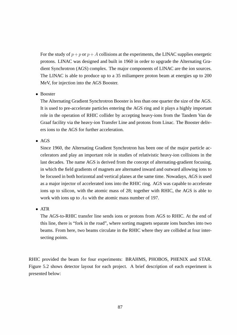
For the study ofp+p or p+A collisions at the experiments, the LINAC supplies energetic

protons. LINAC was designed and built in 1960 in order to upgrade the Alternating Gra-

dient Synchrotron (AGS) complex. The major components of LINAC are the ion sources.

The LINAC is able to produce up to a 35 miliampere proton beam at energies up to 200

MeV, for injection into the AGS Booster.

• Booster

The Alternating Gradient Synchrotron Booster is less than one quarter the size of the AGS.

It is used to pre-accelerate particles entering the AGS ringand it plays a highly important

role in the operation of RHIC collider by accepting heavy-ions from the Tandem Van de

Graaf facility via the heavy-ion Transfer Line and protons from Linac. The Booster deliv-

ers ions to the AGS for further acceleration.

• AGS

Since 1960, the Alternating Gradient Synchrotron has been one of the major particle ac-

celerators and play an important role in studies of relativistic heavy-ion collisions in the

last decades. The name AGS is derived from the concept of alternating-gradient focusing,

in which the field gradients of magnets are alternated inwardand outward allowing ions to

be focused in both horizontal and vertical planes at the sametime. Nowadays, AGS is used

as a major injector of accelerated ions into the RHIC ring. AGSwas capable to accelerate

ions up to silicon, with the atomic mass of 28; together with RHIC, the AGS is able to

work with ions up toAu with the atomic mass number of 197.

• ATR

The AGS-to-RHIC transfer line sends ions or protons from AGS to RHIC. At the end of

this line, there is “fork in the road”, where sorting magnetsseparate ions bunches into two

beams. From here, two beams circulate in the RHIC where they are collided at four inter-

secting points.

RHIC provided the beam for four experiments: BRAHMS, PHOBOS, PHENIX and STAR.

Figure 5.2 shows detector layout for each project. A brief description of each experiment is

presented below:

87

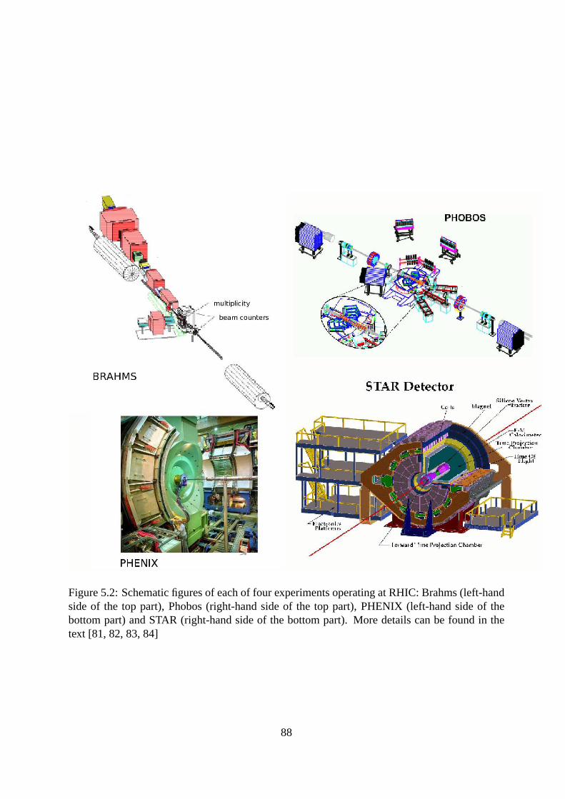
Figure 5.2: Schematic figures of each of four experiments operating at RHIC: Brahms (left-handside of the top part), Phobos (right-hand side of the top part), PHENIX (left-hand side of thebottom part) and STAR (right-hand side of the bottom part). More details can be found in thetext [81, 82, 83, 84]

88

BRAHMS

The Broad Range Hadron Spectrometer experiment [81], designed to measure charged hadrons

over a wide range of rapidity and transverse momentum for allbeams and energies available at

RHIC is already accomplished. The detector requirements at midrapidity and forward angles

are different and the experiment uses two movable spectrometers for these two regions (Figure

5.2). The mid-rapidity spectrometer covers the pseudorapidity range0 < η < 1.3 and the

forward spectrometer covers1.3 < η < 4.0 range. There are four dipole magnets, three time

projection chambers (TPC) and drift chambers. Particle identification is possible via time-of-

flight hodoscopes and Cerenkov counter. The mid-rapidity spectrometer was designed to record

charged particles below momenta of 5 GeV/c.

PHOBOS

This detector [82] was designed to measure as many produced particles as possible and to allow

the detection of particles with lower transverse momenta (Figure 5.2). The experiment is already

accomplished. The detector is composed of two parts: a multiplicity detector covering almost

the entire pseudorapidity range (−5.4 < η < 5.4) measuring total charged particle multiplicitydNch

dηover entire phase-space, and a two-arm spectrometer at mid-rapidity region. For about

1% of the produced particles, information about momentum and particle identification is done

via the spectrometer. Each of the two arms covers about 0.4 rad in azimuth and one unit of

pseudorapidity in the range of0 < η < 2.

PHENIX

This experiment [83] is dedicated to measuring electrons, muons, hadrons and photons. Its

experimental abilities reach the highest event rates, evenup to ten times of RHIC design lumi-

nosities. The goal is to collect rare signals such as theJ/ψ decays into muons and electrons,

high transverse momentumπ0’s, direct photons and many others. The detector is composedof

four spectrometer arms, two central have a small angle coverage at central rapidity region. Each

is built up from a silicon vertex detector, a drift chamber, apixel pad chamber, a ring-imaging

Cerenkov counter, a time-expansion chamber, a time-of-flight and an electromagnetic calorime-

ter. These detectors enable identification of electrons over a broad range of momenta in order

to measure low- and high-mass vector mesons. The other two spectrometers are used for muon

89

detection, and are built up from cathode strip chambers. ThePHENIX experimental setup is

presented in Figure 5.2.

STAR

The Solenoidal Tracker At RHIC (STAR) [84] is another of the four experiments at the RHIC ac-

celerator. STAR has been design to investigate the behaviorof strongly interacting matter at high

energies and to search for signatures of QGP formation. Its goal is to understand fundamental

properties of hadronic matter and its interactions.

5.2 The STAR detector

The STAR layout is shown in Figures 5.2, 5.3. The data collecting is performed in the magnetic

field of up to 0.5T. The main detector used to measure charged hadrons is the Time Projection

Chamber (TPC). It is located at a radial distance of50 to 200cm from the beam axis. The TPC

is 4.2m long and has4m of diameter. TPC is filled with theP10 drift gas (10% methane,90%

argon) regulated at2mbar above atmospheric pressure. The main property of theP10 gas is

its fast drift velocity in low electric field. The drift velocity is stable and insensitive to small

variations in temperature and pressure. The uniform low electric field is135V/cm. The paths of

primary ionizing particles passing through the gas volume are reconstructed with high precision

from released secondary electrons, which drift to the readout end caps. Electric field uniformity

is critical to the order ofmm and electron drift paths are up to2m long.

In order to increase the TPC acceptance, the tracking is extended to the forward region using two

radial-drift TPCs. The combination of the TPC and the tag two FTPC covers−1.8 < η < 1.8

with complete azimuthal symmetry (∆φ = 2π), over the full range of multiplicities. The TPC

records tracks of particles, measures their momentum and identifies the particles by estimating

their ionization loss (dE/dx)- (see more details in Chapter 5.3). Particles are best identified in

their momentum range of100 MeV/c to 1GeV. Momenta without particle identification can be

measured up even to30 GeV/c.

Charged particles produced close to the interaction region are identified via sub-detectors: the

Silicon Vertex Tracker (SVT) and the Silicon Strip Detector(SSD). The silicon detectors cover

the pseudo-rapidity range of−1 < η < 1 with complete azimuthal symmetry (∆φ = 2π) and

they can find secondary vertices from weak decays of hyperons, e.g.Λ, Ξ, Ω. In order to extend

90

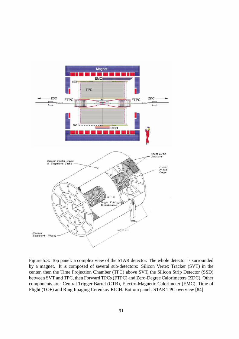
Figure 5.3: Top panel: a complex view of the STAR detector. The whole detector is surroundedby a magnet. It is composed of several sub-detectors: Silicon Vertex Tracker (SVT) in thecenter, then the Time Projection Chamber (TPC) above SVT, the Silicon Strip Detector (SSD)between SVT and TPC, then Forward TPCs (FTPC) and Zero-Degree Calorimeters (ZDC). Othercomponents are: Central Trigger Barrel (CTB), Electro-Magnetic Calorimeter (EMC), Time ofFlight (TOF) and Ring Imaging Cerenkov RICH. Bottom panel: STAR TPC overview [84]

91

the particle identification to larger momenta for identifiedsingle-particle spectra at midrapidity, a

ring imaging Cerenkov detector covering−0.3 < η < 0.3 and∆φ = 0.11π and Time-Of-Flight

(TOF) with coverage−1.0 < η < 1.0 and∆φ = 0.04π were installed. STAR has the ability to

detect hadrons in large detector acceptance, it is also ableto measure event-by-event fluctuations

and jets.

5.3 Performance of TPC

The STAR detector uses the TPC as its primary tracking device. All results of data analysis

presented in this work use data reconstructed by the TPC detector only. The STAR TPC is

presented in Figure 5.3 (bottom panel).

The track of a finite momentum particle passes through the TPCand can reach up to 45 pad-

rows. A finite momentum track rarely crosses all rows, it depends on the radius of curvature

of the track, the track pseudorapidity, cuts nearby sector boundaries and few more other details

about particle trajectory. While the wire chamber is sensitive to almost100% of the secondary

electrons, the overall tracking efficiency is lower (80-90%) due to cuts, track merging, bad pads

and dead channels. There is a few percent of dead channels in any run cycle.

The track of a primary particle passing through the TPC is reconstructed by finding ionization

clusters along the track. The clusters are found separatelyin x, y andz directions. The local

x axis is along the direction of the pad-row, the localy axis extends from beam-line outward

through the middle of an perpendicular to the pad-rows, the localz axis lies along the beam axis.

These clusters are split using an algorithm then looks for peaks with a valley between them and

then ionization is divided between the two tracks. Below, experimental details concerning the

track reconstruction and its imperfections are explained.

Distortions

The position of a secondary electron in a pad can be distortedby non-uniformities in the electric

and magnetic field of the TPC. The non-uniformities in the fieldlead to non-uniform drift. In

the STAR TPC, the electric and magnetic fields are parallel andnearly uniform inr andz. The

deviations from these ideal conditions are small and a typical distortion along the pad row is≤ 1

mm before applying a correction. The magnitude of differentdistortion corrections are presented

in the Table 5.1.

92

Table 5.1: The distortion corrections applied to STAR data,their cause and the magnitude oftheir effect on the data

Cause of the Distortion Magnitude of theImperfection

Magnitude of theCorrection

Non-uniform B field ±0.004 T .. leads to∼0.1 cmGeometrical effect

between the inner andouter sub-sectors

Exact calculation basedon geometry

0.005

The angular offsetbetween E and B field

0.2 mr 0.03 cm

TPC endcaps - non-flatshape and tilt

0.1 cm 0.03 cm

Two-hit resolution

The efficiency of two-hit resolution is the ratio of the distributions of the distance separating2

hits from the same event and2 hits from different events. Two hits can be completely resolved

when they are separated in the pad-row direction by at least0.8 cm in the inner sector and1.3

cm in the outer sector. Similarly, two hits are completely resolved when they are separated in the

drift direction by2.7cm in the inner sector and3.2cm in the outer one.

Tracking efficiency

The tracking software performs two distinct tasks: the algorithms associate space-points to form

tracks and fit the points on a track with a track model to extract information such as the momen-

tum of particle. The track model is a helix. Second-order effects include the energy lost in the

gas which causes a particle trajectory to deviate slightly from the helix.

The tracking efficiency depends on the acceptance of the detector and the two-hit separation ca-

pability of the system. The acceptance is96% for high-momentum tracks traveling perpendicular

the beam. The4% inefficiency is caused by the spaces between sectors which have to exist due

to the wires on the sectors. The software also ignores any space-points that fall on the last2 pad-

rows. This cut is applied to avoid position errors that result from tracks not having symmetric

pad coverage on both sides of the track. It also allows to avoid local distortions in the drift field,

so the total acceptance is94 %.

The detection efficiency of the electronics is almost100% except for dead channels (they count

93

below1% of the total amount). However, the system cannot always distinguish one hit from two

hits and this merging reduces tracking efficiency. In order to estimate the tracking efficiency,

simulated tracks are embedded inside real events and then the number of simulated tracks that

are in the data after track reconstruction are counted. Thistechnique allows to account for detec-

tor effects and especially for the losses related to a high density of tracks. The simulated tracks

are very similar to the real tracks and simulator tries to take into account all the processes that

lead to the detection of particles including: ionization, electron drift, gas gain, signal collection,

electronic amplification, electronic noise and dead channels. The results of embedding studies

indicate that systematic error on the tracking efficiency isabout6%.

Vertex resolution

The primary vertex can be used to improve the momentum resolution of tracks and to distinguish

secondary vertices from the primary ones. It is also possible to improve the momentum resolution

of secondary vertices as well, however the vertex resolution has to be good enough. Many strange

particles produced in heavy-ion collisions can be identified this way. The primary vertex is found

by considering all of the tracks reconstructed in the TPC andthe extrapolating them back to the

origin. The global average corresponds to the the vertex position. The primary vertex resolution

is calculated by comparing the position of the vertices thatare reconstructed using each side of

TPC separately. As expected, the resolution decreases as the square root of the number of tracks

used in calculations. A resolution of350µm is achieved when more than1000 tracks exist.

Momentum resolution

The transverse momentumpT of a track is measured by fitting a circle through thex, y coor-

dinates of the vertex and the points along the track. The total momentum is calculated using

this radius of track curvature and the angle of the tracks with respect to thez- axis of the TPC.

This procedure works for all primary particles coming from the vertex, but for secondary decays,

such aΛ or K0s , the circle must be done without reference to the primary vertex first. In order

to estimate the momentum resolution, it is necessary to apply the embedding technique. A track

simulator is used to create a track with known momentum, thenthe track is embedded in real

event in order to simulate the momentum smearing effects. There are two regions of low resolu-

tion: lower-pT domain: for e.g. pions - forpT < 400 MeV/c, for anti-protons -pT < 600 MeV/c,

94

Figure 5.4: Transverse momentum resolution of the STAR TPC for negative pions and anti-protons in the magnetic field0.25T. Tracks are required to be built up from more than15 hits.Tracks are embedded in minimum bias events [84].

and higher-pT domain where the momentum is limited by the strength of the magnetic field and

the TPC spatial resolution (see Figure 5.4).

Particle identification using dE/dx

Energy loss in the TPC is a valuable tool to identify particlespecies. It works especially well

for low momentum particles but as the particle energy increases, the energy loss becomes less

mass dependent and it is highly difficult to separate particles with their momenta above several

GeV/c. STAR is able to separate pions, kaons and protons witha very good accuracy up to1.2

GeV/c. Above this region, the accuracy is much lower, but separation is still possible, up to the

momentum above10 GeV. The best separation requires a relative momentum resolution of the

order of7%. ThedE/dx loss is extracted from the energy loss measured on up to45 pad-rows.

The procedure to get particle characteristics (momentum, energy, ..) is the offline analysis which

consists of several parts:

• Digital and analog signals (hits) are read from the detectorclusters. Using known cali-

bration constants, any signal is converted into space-timecoordinates of a given cluster

95

(x,y,z,t).

• Tracks are assembled from read clusters.

• A global track can be formed from several segments (tracks) of the analyzed part of the

detector.

• With a global track present, it is extrapolated to the primary vertex. A fit to the primary

vertex can be done using the values of the magnetic field.

• The velocity coordinates are specified and when the mass of particle which left a track at

that moment is known- the momentum coordinates are given as well.

• In the case of non-primordial particles (decayed from otherparticle), the reconstruction of

secondary vertices and other particle daughters can be found.

• The Bethe-Bloch formula on energy loss is given:

−dE

dx=

4π

mec2

nz2

β2(

e2

4πǫ0

)2[ln2mec

2β2

I(1 − β2)− β2] (5.1)

whereE is the energy,x is the distance unit where the energy is losses;β = vc

(v is the

particle velocity,c is the speed of light);me is the mass of electrone; z is the charge of

particle; n is the density of electrons inside the mediumn = NAZρA

(NA is Avogadro’s

number;A, Z corresponds to the atomic properties of the element which the medium is

built of; ρ is the density of the medium);I = (10eV)Z is the ionization potential of the

medium.

The measureddE/dx resolution depends on the gas gain which itself depends on the pressure

in the TPC. Since the TPC is kept at a constant value of2 mbar above atmospheric pressure, the

TPC pressure varies with time. There are small variations between pads and groups of pads, due

to the different response of each readout board.

The length over which the particle energy loss is measured (depending on: pad length, crossing

and dip-angle) is too short to average out ionizations fluctuations. Indeed, particles lose the

energy in collision with the gas. It is not possible to measure accurately the average ofdE/dx,

96

Figure 5.5: The energy loss distribution in the STAR TPC as a function of transverse momentum.The magnetic field is0.25T. The resolution of8% of a track that crosses40 pad-rows. Bothprimary and secondary particles are included. Pions, kaons, protons can be separated from eachother up to1GeV/c. The electron band contaminates mostly sample of pions, kaons and protonsfor higher momenta [84].

so the mean energy losses are distinguished. They are parametrized according to the Landau

distribution. The energy is measured for multiple points ofthe track, then the energy lossesdEdx

can be calculated (truncated mean). Figure 5.5 shows the energy loss for particles in the TPC

detector.

More about the main STAR detector TPC can be found in [85].

Experimental details related to proton femtoscopy analysis are described in the next Section 6.

97

Chapter 6

Analysis of two-baryon correlations

6.1 Construction of two-particle correlation function

In order to build up any correlation function, a proper selection of correlated particles must be

applied. Collection of correlation function constituents is done on three different levels:

• events,

• particles,

• pairs.

Proper event selection is highly important for correct background construction. A correlation

function is usually calculated by dividing two-particle distributions coming from the same event

(in numerator) and from different events (in denominator),where the latter- the background sam-

ple should be a "perfect reference", reflecting an ideal scenario of non-correlated particles. On

the other hand, this sample should preserve some geometrical correlations resulting e.g. from the

collision geometry (physics) and detector configuration (measurement). It is not enough to mix

particles from any different events- they should exhibit similar properties concerning position as

the vertex in the detector along the beam axis, as well as multiplicity (events should be character-

ized by comparable centrality of the collision). A commonlyused, simple-to-calculate variable

which enables estimation of the centrality class is a percentage of total hadronic cross-section

of the collision. For this analysis,20 million minimum-bias events have been selected with the

collision vertex position within±30 cm measured along the beam axis from the center of TPC.

98

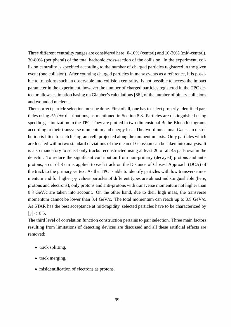
Three different centrality ranges are considered here: 0-10% (central) and 10-30% (mid-central),

30-80% (peripheral) of the total hadronic cross-section ofthe collision. In the experiment, col-

lision centrality is specified according to the number of charged particles registered in the given

event (one collision). After counting charged particles inmany events as a reference, it is possi-

ble to transform such an observable into collision centrality. Is not possible to access the impact

parameter in the experiment, however the number of charged particles registered in the TPC de-

tector allows estimation basing on Glauber’s calculations[86], of the number of binary collisions

and wounded nucleons.

Then correct particle selection must be done. First of all, one has to select properly-identified par-

ticles usingdE/dx distributions, as mentioned in Section 5.3. Particles are distinguished using

specific gas ionization in the TPC. They are plotted in two-dimensional Bethe-Bloch histograms

according to their transverse momentum and energy loss. Thetwo-dimensional Gaussian distri-

bution is fitted to each histogram cell, projected along the momentum axis. Only particles which

are located within two standard deviations of the mean of Gaussian can be taken into analysis. It

is also mandatory to select only tracks reconstructed usingat least 20 of all 45 pad-rows in the

detector. To reduce the significant contribution from non-primary (decayed) protons and anti-

protons, a cut of 3 cm is applied to each track on the Distance of Closest Approach (DCA) of

the track to the primary vertex. As the TPC is able to identifyparticles with low transverse mo-

mentum and for higherpT values particles of different types are almost indistinguishable (here,

protons and electrons), only protons and anti-protons withtransverse momentum not higher than

0.8 GeV/c are taken into account. On the other hand, due to their high mass, the transverse

momentum cannot be lower than0.4 GeV/c. The total momentum can reach up to0.9 GeV/c.

As STAR has the best acceptance at mid-rapidity, selected particles have to be characterized by

|y| < 0.5.

The third level of correlation function construction pertains to pair selection. Three main factors

resulting from limitations of detecting devices are discussed and all these artificial effects are

removed:

• track splitting,

• track merging,

• misidentification of electrons as protons.

99

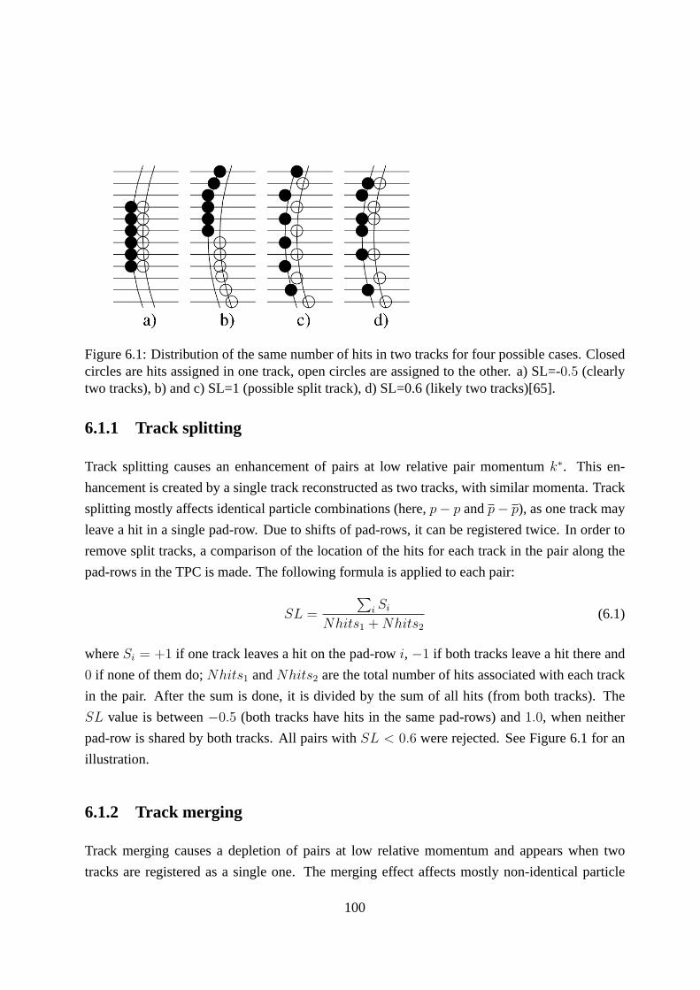
Figure 6.1: Distribution of the same number of hits in two tracks for four possible cases. Closedcircles are hits assigned in one track, open circles are assigned to the other. a) SL=-0.5 (clearlytwo tracks), b) and c) SL=1 (possible split track), d) SL=0.6(likely two tracks)[65].

6.1.1 Track splitting

Track splitting causes an enhancement of pairs at low relative pair momentumk∗. This en-

hancement is created by a single track reconstructed as two tracks, with similar momenta. Track

splitting mostly affects identical particle combinations(here,p − p andp − p), as one track may

leave a hit in a single pad-row. Due to shifts of pad-rows, it can be registered twice. In order to

remove split tracks, a comparison of the location of the hitsfor each track in the pair along the

pad-rows in the TPC is made. The following formula is appliedto each pair:

SL =

∑

i Si

Nhits1 + Nhits2

(6.1)

whereSi = +1 if one track leaves a hit on the pad-rowi, −1 if both tracks leave a hit there and

0 if none of them do;Nhits1 andNhits2 are the total number of hits associated with each track

in the pair. After the sum is done, it is divided by the sum of all hits (from both tracks). The

SL value is between−0.5 (both tracks have hits in the same pad-rows) and1.0, when neither

pad-row is shared by both tracks. All pairs withSL < 0.6 were rejected. See Figure 6.1 for an

illustration.

6.1.2 Track merging

Track merging causes a depletion of pairs at low relative momentum and appears when two

tracks are registered as a single one. The merging effect affects mostly non-identical particle

100

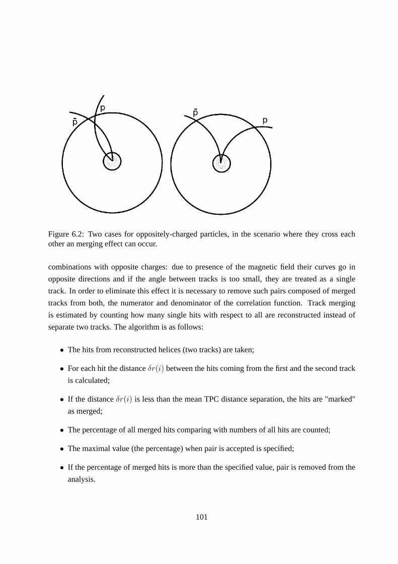
Figure 6.2: Two cases for oppositely-charged particles, inthe scenario where they cross eachother an merging effect can occur.

combinations with opposite charges: due to presence of the magnetic field their curves go in

opposite directions and if the angle between tracks is too small, they are treated as a single

track. In order to eliminate this effect it is necessary to remove such pairs composed of merged

tracks from both, the numerator and denominator of the correlation function. Track merging

is estimated by counting how many single hits with respect toall are reconstructed instead of

separate two tracks. The algorithm is as follows:

• The hits from reconstructed helices (two tracks) are taken;

• For each hit the distanceδr(i) between the hits coming from the first and the second track

is calculated;

• If the distanceδr(i) is less than the mean TPC distance separation, the hits are "marked"

as merged;

• The percentage of all merged hits comparing with numbers of all hits are counted;

• The maximal value (the percentage) when pair is accepted is specified;

• If the percentage of merged hits is more than the specified value, pair is removed from the

analysis.

101

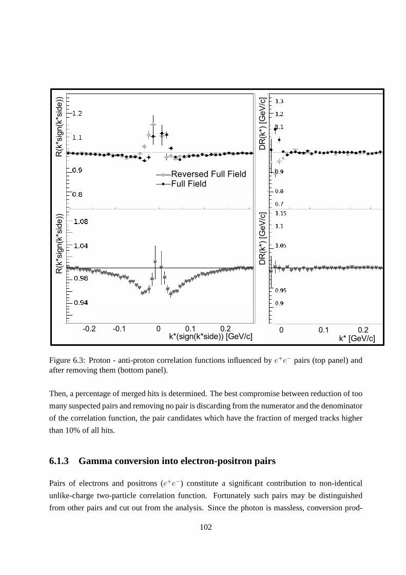
Figure 6.3: Proton - anti-proton correlation functions influenced bye+e− pairs (top panel) andafter removing them (bottom panel).

Then, a percentage of merged hits is determined. The best compromise between reduction of too

many suspected pairs and removing no pair is discarding fromthe numerator and the denominator

of the correlation function, the pair candidates which havethe fraction of merged tracks higher

than 10% of all hits.

6.1.3 Gamma conversion into electron-positron pairs

Pairs of electrons and positrons (e+e−) constitute a significant contribution to non-identical

unlike-charge two-particle correlation function. Fortunately such pairs may be distinguished

from other pairs and cut out from the analysis. Since the photon is massless, conversion prod-

102

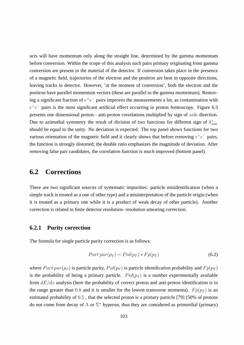
ucts will have momentum only along the straight line, determined by the gamma momentum

before conversion. Within the scope of this analysis such pairs primary originating from gamma

conversion are present in the material of the detector. If conversion takes place in the presence

of a magnetic field, trajectories of the electron and the positron are bent in opposite directions,

leaving tracks in detector. However, ’at the moment of conversion’, both the electron and the

positron have parallel momentum vectors (these are parallel to the gamma momentum). Remov-

ing a significant fraction ofe+e− pairs improves the measurements a lot, as contamination with

e+e− pairs is the most significant artificial effect occurring in proton femtoscopy. Figure 6.3

presents one dimensional proton - anti-proton correlations multiplied by sign ofside direction.

Due to azimuthal symmetry the result of division of two functions for different sign ofk∗

side

should be equal to the unity. No deviation is expected. The top panel shows functions for two

various orientation of the magnetic field and it clearly shows that before removinge+e− pairs,

the function is strongly distorted; the double ratio emphasizes the magnitude of deviation. After

removing false pair candidates, the correlation function is much improved (bottom panel).

6.2 Corrections

There are two significant sources of systematic impurities:particle misidentification (when a

simple track is treated as a one of other type) and a misinterpretation of the particle origin (when

it is treated as a primary one while it is a product of weak decay of other particle). Another

correction is related to finite detector resolution- resolution smearing correction.

6.2.1 Purity correction

The formula for single particle purity correction is as follows:

Part pur(pT ) = Pid(pT ) ∗ Fp(pT ) (6.2)

wherePart pur(pT ) is particle purity,Pid(pT ) is particle identification probability andFp(pT )

is the probability of being a primary particle.Pid(pT ) is a number experimentally available

from dE/dx analysis (here the probability of correct proton and anti-proton identification is in

the range greater than0.8 and it is smaller for the lowest transverse momenta).Fp(pT ) is an

estimated probability of0.5 , that the selected proton is a primary particle [79] (50% of protons

do not come from decay ofΛ or Σ∗ hyperon, thus they are considered as primordial (primary)

103

protons). The calculation is based on HIJING predictions [42] for transverse momenta[0.4, 0.8]

GeV/c (as the highest proper proton and anti-proton identification probabilities are estimated in

this interval). In the terms of a pair:

Pair pur(k∗) = Part pur1(pT1) ∗ Part pur2(pT2) (6.3)

wherePair pur(k∗) is a pair purity product of multiplying separate probabilities for single par-

ticles part1 andpart2. Pair pur(k∗) is a histogram which depends on many combinations of

pT1 andpT2. In the terms of a pair, the probability that a pair is composed of primordial particles

is 0.25 (not taking into account the track misidentification). Corrected correlation functions are

calculated according to the formula:

Ccorr(k∗) =

Cmeas(k∗) − 1

Pair pur(k∗)+ 1 (6.4)

6.2.2 Resolution smearing correction

Momentum resolution is parametrized in the following way:

pi

pi

= ap,i + bp,ipαi

i + cp,ipi (6.5)

φi = aφ,i + bφ,iφαi

i (6.6)

θ = aθ,i + bθ,iθαi

i (6.7)

wherei denotes a particle type. For each particle, basing on its momentump and anglesφ and

θ (the azimuthal angle with respect to the horizontal plane and the polar angle between the track

and beam axis, respectively), corresponding smeared sigmasσ p, σ φ andσ θ are found.

Then, momentum resolution smears∂p, ∂φ and∂θ are generated, from Gaussian distributions

with zero mean values and corresponding sigmas; new, smeared momenta are calculated:

psmearx = pmeas

x + ∂px (6.8)

psmeary = pmeas

y + ∂py (6.9)

psmearz = pmeas

z + ∂pz (6.10)

104

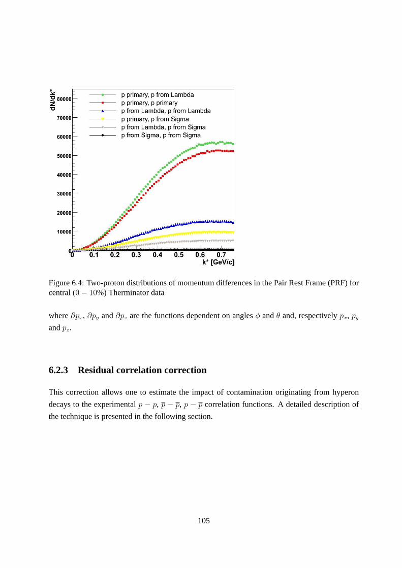
Figure 6.4: Two-proton distributions of momentum differences in the Pair Rest Frame (PRF) forcentral (0 − 10%) Therminator data

where∂px, ∂py and∂pz are the functions dependent on anglesφ andθ and, respectivelypx, py

andpz.

6.2.3 Residual correlation correction

This correction allows one to estimate the impact of contamination originating from hyperon

decays to the experimentalp − p, p − p, p − p correlation functions. A detailed description of

the technique is presented in the following section.

105

6.3 Residual correlations

6.3.1 Basics of residual correlation effects

The motivation of these studies is that preliminary resultson proton femtoscopy indicated two

source sizes: one for identical particles and the other one for non-identical particle species. The

radii for p − p andp − p are consistent within each centrality bin, however the source size for

p − p is considerably smaller. These observables agree for two collision energies:62 and200

GeV. Then again, these results are obtained without taking into account the effect of residual

correlations arising due to baryons decaying into protons and anti-protons.

From the experimental point of view, many secondary protonsand anti-protons are indistinguish-

able from primordial particles, as their parent particles are not detected. Neglecting this fact leads

to misinterpretation of the results, where instead ofp−p interactions, correlations between other

particles (which decayed finally into proton) are observed.Two main weak decay channels are

the most important:

Λ → p + π− (6.11)

Σ+ → p + π0 (6.12)

In fact, all Residual Correlations (RCs) arising from decay channels which lead to proton (anti-

proton) through hyperons are considered. In order to evaluate the effect of RCs occurring in pro-

ton femtoscopy, this analysis uses the Therminator (THERMalheavy-ion GenerATOR) Monte

Carlo event generator [87, 88], a generator designed to studyparticle production at SPS, RHIC

and LHC energies. This program implements a thermal model ofparticle production with a sin-

gle freeze-out. The geometry of the freeze-out hypersurface is chosen according to the Cracow

model [89, 90] and the space-time emission point, as well as parent information is stored for

each particle. These studies are centrality dependent, which means that for each centrality class,

a separate sample of Therminator events is generated. Figures 6.4-6.7 present the results for

central events.

6.3.2 Combining contributions from several sources

The experimentally measured proton - proton (and anti-proton - anti-proton) correlations are

described by the Equation 6.13. It includes all pair combinations, taking into account both (ex-

106

Figure 6.5: The fraction of pairs composed of primordial particles: proton - proton (blacksquares), anti-proton - anti-proton (dark gray circles), and proton - anti-proton (bright stars)for central (0 − 10%) Therminator collisions

pressions 6.11 and 6.12) decay channels:

Ctrue(k∗) = Cp−p(k

∗)Fp−p(k∗) + Cp−Λ(k∗)Fp−Λ(k∗) + CΛ−Λ(k∗)FΛ−Λ(k∗)

+Cp−Σ(k∗)Fp−Σ(k∗) + CΣ−Σ(k∗)FΣ−Σ(k∗) + CΛ−Σ(k∗)FΛ−Σ(k∗)

(6.13)

whereFx−y(k∗) represents the fraction of measuredp − p pairs, where most primary parents

werex andy. In order to evaluate the fractionsFx−y(k∗) of each type of correlation, all protons

are divided into three groups: primordial particles, protons coming fromΛ hyperons and ones

coming from decays ofΣ+ baryons. It is calculated as the number ofx − y pairs (dependent

on k∗) with respect to all pairs (e.g ifx, y mean primary protons, thenFp−p(k∗) is calculated as

a number of allp − p pairs, where both particles are primary ones and their number is scaled

by the number of allp − p pairs, where the origin of first and second proton does not matter).

For all two-proton combinations,k∗ distributions are computed (Figure 6.4). The dominant

contribution for allk∗ values, comes fromp − Λ pairs, indicating thatp − Λ residual interaction

strongly affects measuredp − p correlation. The presence of other types of residual correlations

107

is much less significant.Cx−y(k∗) means the residual contribution ofx−y correlation (explained

in the next sub-section).Ctrue(k∗) is the experimentally measured correlation function corrected

for particle identification probability (PID) purity. The aim of this study is to estimate the pure

p−p correlation (Cp−p(k∗) from Equation 6.13) after removing the residual ones. The fraction of

pure correlation is slightlyk∗- dependent function, with the mean value from 0.31 (for thep − p

system) to 0.38 (for thep − p system), due top/p ratio smaller thanΛ/Λ ratio. These numbers

correspond to central events. The main weak-decay channelsof protons and anti-protons are

lambda and anti-lambda ones. The fractions of pure correlations are shown in Figure 6.5.

The formula for thep − p system is a little more complicated as it contains all combinations of

protons and anti-protons from 6 different groups. The mechanism of calculating the RCs existing

in p − p systems is not described here as it is similar to the one for identical proton femtoscopy.

6.3.3 Convolution of decay kinematics

Thep − Λ correlation function is measured by STAR [79] as a function of k∗

p−Λ. However the

argument ofCp−Λ in Equation 6.13 isk∗

p−p, the relative momentum between two protons; in this

case, one of the protons is the decay daughter ofΛ. To calculate thep − Λ contribution to the

measuredp − p correlation function, thep − Λ correlation function must be convoluted with

Λ-decay kinematics. Figure 6.6 shows regions ofk∗

p−Λ, where thep − Λ RC affect some ranges

of k∗

p−p. This figure presents results for central collisions. For each value ofk∗

p−p, the influence of

thep−Λ correlation is computed (Equation 6.14) as a sum over allk∗

p−Λ bins, of experimentally

measuredp − Λ correlations scaled by the factors from theW (k∗

p−p, k∗

p−Λ) histogram.

Cp−Λ(k∗

p−p) =∑

k∗

p−Λ

Cmeasp−Λ (k∗

p−Λ)W (k∗

p−p, k∗

p−Λ) (6.14)

The p − Λ correlation should not be corrected for purity, as it contains residual correlations

derived from higher-order decays. For mid-central and peripheral collisionsp − Λ (andp − Λ)

correlation functions are analytically calculated using the Lednicky & Lyuboshitz model [78],

assuming scaling ofp − Λ (andp − Λ) radii according to scaling ofp − p (andp − p) source

sizes before applying RC corrections. RCs fromp − Σ+ andΣ+ − Σ+ channels are assumed to

arise only from Coulomb interactions for all systems, in addition to QS forΣ+ − Σ+. The (k∗

p−p

andk∗

p−Σ+), (k∗

p−p andkΣ+−Σ+) kinematic dependencies of decay ofΣ+ hyperons are considered

separately. In the case ofΛ − Λ andΛ − Σ+ interactions no correlation is assumed, therefore

for eachk∗ value a flat distribution is equal to unity. In these systems strong FSI occur (and

108

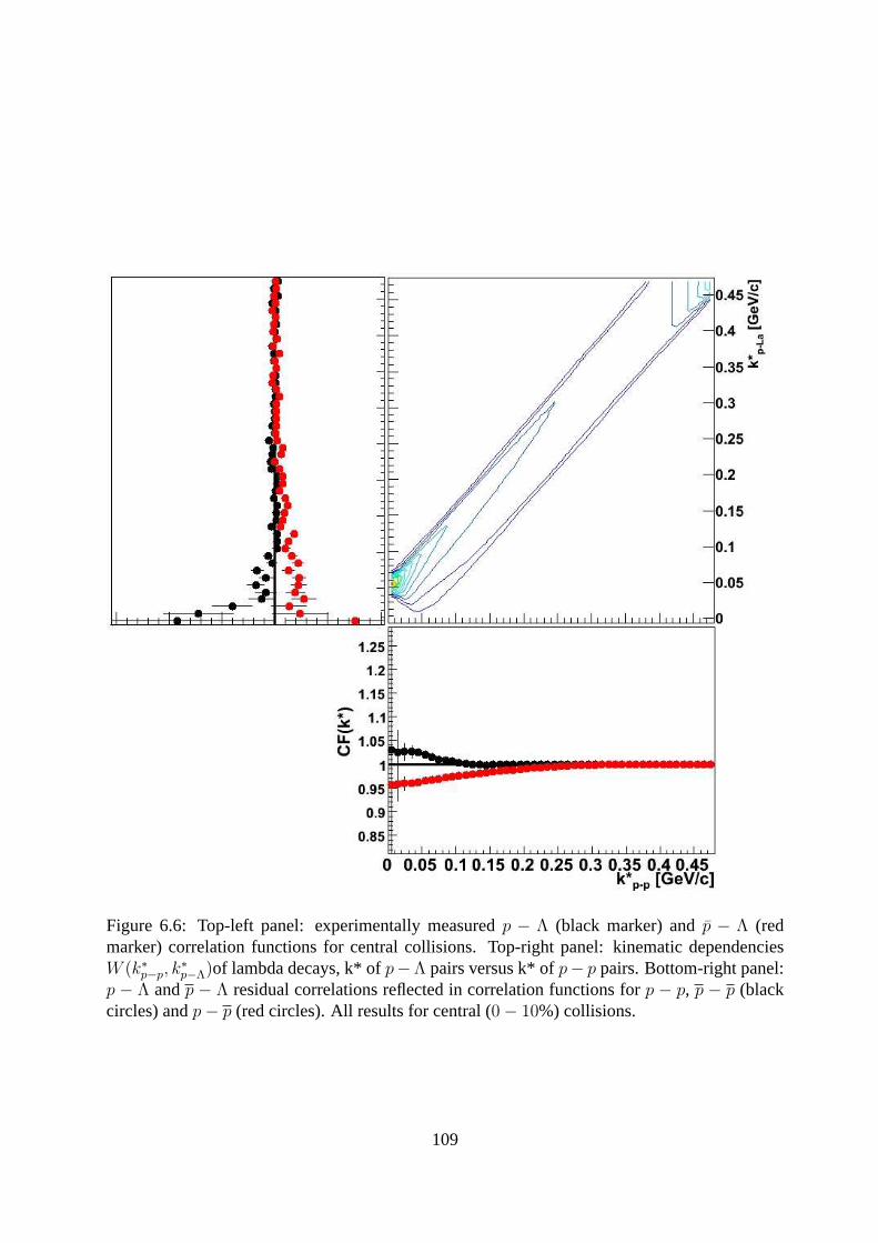
Figure 6.6: Top-left panel: experimentally measuredp − Λ (black marker) andp − Λ (redmarker) correlation functions for central collisions. Top-right panel: kinematic dependenciesW (k∗

p−p, k∗

p−Λ)of lambda decays, k* ofp−Λ pairs versus k* ofp− p pairs. Bottom-right panel:p − Λ andp − Λ residual correlations reflected in correlation functions for p − p, p − p (blackcircles) andp − p (red circles). All results for central (0 − 10%) collisions.

109

Figure 6.7: Residual correlations in proton - proton (top panel) and proton - anti-proton (bottompanel) system for central collisions (0-10%). The differences between red (uncorrected) andblack circles (corrected for residual correlations) show the importance of residual correlationcorrection. 110

QS inΛ − Λ system as well); their existing theoretical descriptions are not confirmed so far by

any experiment, thus should not be taken into account. On theother hand, the impact of RCs

coming from these combinations do not contribute to the purep−p correlation such significantly

asp − Λ system, so assuming no correlation for these cases is much appropriate than assuming

some correlation. If such correlation would be predicted (if Λ−Λ correlation would be known),

one should consider proper source size. At the moment it is not clear how to estimate the shape

of Λ − Λ correlations correctly.

In these studies onlyp−Λ (andp−Λ) are taken from experiment. Correlating processes for other

systems are estimated if the calculation of QS and Coulomb interaction is possible to perform.

Estimation of strong-interaction parameters for systems like: Λ−Λ, (Λ−Λ), Σ+−Σ+ (Σ+−Σ+),

andΛ − Σ (Λ − Σ+) is highly non-trivial and is not included in these studies;however, it does

not add significant discrepancies as fractions of such RCs are not large (see Figure 6.4).

6.3.4 Effects on extracted length scales

The net effect of the purity and RC corrections is shown in Figure 6.5. All correlation functions

are corrected for Particle IDentification (PID) effects (more in Section 7). Here, the first estimate

of the fraction of primary-primary proton pairs was0.25 (i.e. fraction of of primary protons0.5);

the correlation function corrected for this purity is shownby open circles in Figure 6.5 forp − p

(top panel) andp − p (bottom panel). A better calculation of pair purity (fractionFp−p(k∗) from

Equation 6.13) is shown by correlation functions marked by red circles. Finally, the extracted

correlation is further reduced when RCs are also corrected for(black circles).

Since thep − Λ correlation is much stronger and wider than thep − Λ one, the residual effects

on thep − p system are more significant than those forp − p system. This is clear in Figure 6.7,

where the effects of various corrections onp − p are shown.

111

Chapter 7

Experimental results

The presentation of experimental results is divided into three sub-sections: the first one (7.1)

contains results without a precise estimation of the effectof RCs, the second sub-section (7.2)

discusses this problem with more details included. Within each part two kinds of corrections are

gradually applied: estimation of impurities and resolution smearing effects. The last sub-section

(7.3) treats non-identical proton - anti-proton correlations in terms of asymmetry analysis in order

to discuss possible differences in the emission process between protons and their anti-particles.

7.1 Two-proton correlations without residual correlation cor-

rections

7.1.1 Raw data

The first step in the analysis of two-particle correlations is to obtain the correlation functions

free of experimental distortions. Some experimental effects, as e.g.: track merging, track split-

ting, contamination with electron - positron pairs coming from photon conversion, can be easily

removed at the level of pair selection. However, there are few imperfections which cannot be

removed during raw-data analysis: falsely identified tracks of particles, resolution smearing of

single tracks, and contamination with non-primary particles. These contaminations are espe-

cially important for baryon correlations, as many of them come from weak decays.

Figure 7.1 shows two - proton, two - anti-proton and proton - anti-proton correlation functions

without corrections for resolution smearing and purity. Asmentioned, the effects of track split-

112

Figure 7.1: Results of proton femtoscopy with no correction applied: proton - proton (top-leftpanel), anti-proton - anti-proton (top-right panel) and proton - anti-proton (bottom-left panel).

113

ting, track merging and electron - positron contamination were removed in the course of data

analysis. The results for identical particle combinationsagree with each other within each cen-

trality bin and follow similar trends, as expected. The correlation functions for central collisions

are weaker than for non-central ones, thus their source sizes are bigger. The correlation effect is

the strongest while considering more peripheral collisions. The top-left panel illustrates proton

- proton correlations for three centralities (up to 10%, 10 -30%, 30 - 80% of the total hadronic

cross section of the collision), the top-right panel shows anti-proton - anti-proton correlations

and the bottom-left panel presents proton - anti-proton correlation functions. Even if none of

the functions are corrected for such impurities, a clear centrality dependence can be observed.

In the case of non-identical particle combinations, annihilation processes between particles and

their anti-particles are observed as well; this effect can be seen as an anti-correlation (below the

value of1.0). Presented in Figure 7.1 are the raw correlation functions, treated as a base for

further corrections. The best source-size fits are not calculated, as the functions need to be scaled

according to many correcting factors.


Due to corrections for purity, comparing to the raw correlation functions, the correlation effects

become stronger and thus their source sizes are smaller. Including statistical and systematic

errors, the results of fit are stored in Table 7.1. The systematic uncertainties are estimated from

the discrepancy of correction for purity. Stability of the fit (for 100% of the applied purity

correction) is checked by estimation of fitted source sizes while applying from90% to 110% of

the correction.

Table 7.1: Source sizes [fm] for different proton combinations and centralities; withpuritycorrections applied; reported errors are respectively, statistical and systematic (due to puritycorrection applied)

p − p [fm] p − p [fm] p − p [fm]

peripheral 2.52+0.11−0.05−0.11−0.05 2.53+0.13+0.08

−0.13−0.07 1.62+0.12+0.05−0.12−0.05

mid − central 3.59+0.09+0.04−0.09−0.04 3.51+0.09+0.07

−0.09−0.07 2.13+0.10+0.03−0.10−0.04

central 4.02+0.07+0.05−0.07−0.06 4.47+0.08+0.07

−0.08−0.06 2.61+0.09+0.03−0.09−0.03

An agreement between identical particle combinations is observed, except for central collisions,

where the source size of the anti-proton - anti-proton correlation is half offm bigger than the

source size of the proton - proton correlation. The discrepancy can be explained as an effect of

114

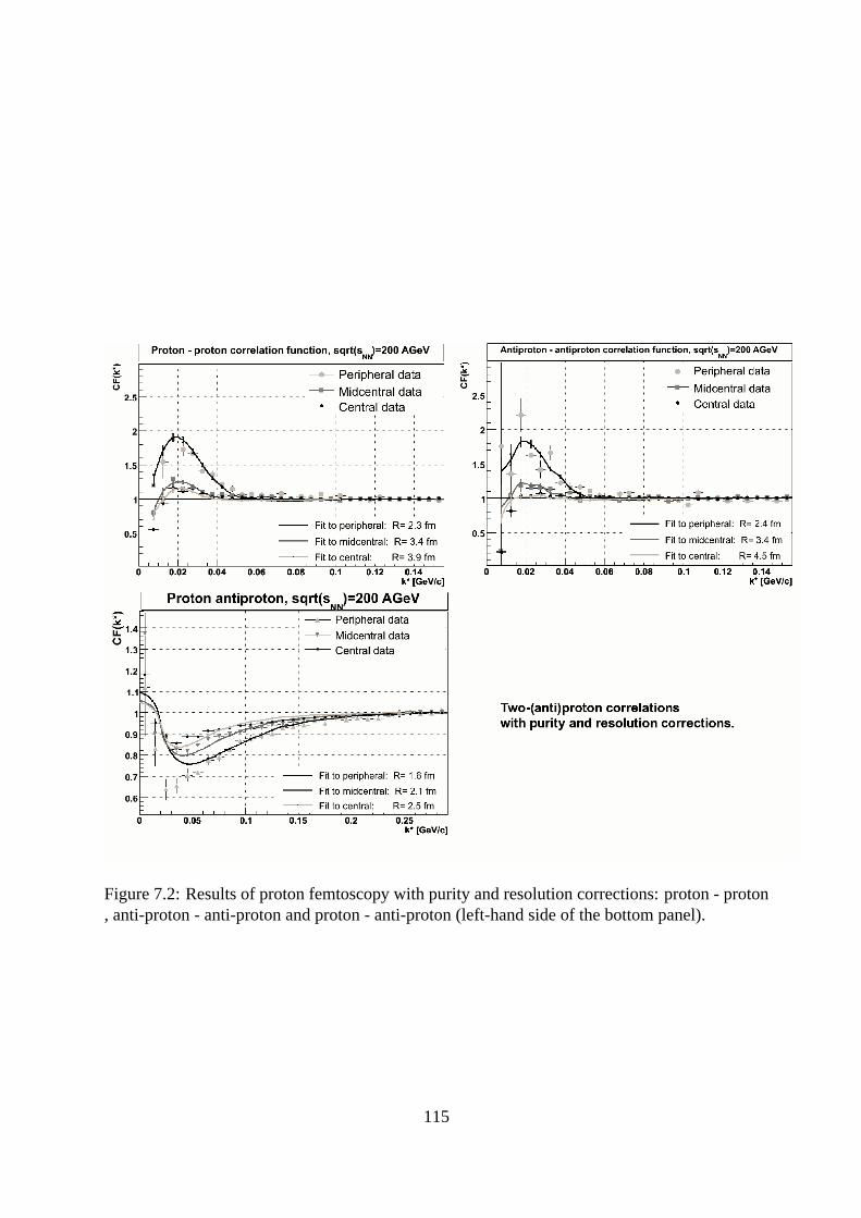
Figure 7.2: Results of proton femtoscopy with purity and resolution corrections: proton - proton, anti-proton - anti-proton and proton - anti-proton (left-hand side of the bottom panel).

115

the weakness of the signal for central collisions. As the source size becomes larger, the corre-

lation becomes weaker and estimation of the source size of the order of4 − 5fm becomes more

difficult. Another interesting difference between the fitted sources is that one between identical

and non-identical particle combinations. In results forp − p andp − p, only for a very small

difference between protons and anti-protons is detected. For these two systems the same source

sizes are expected. The proton - anti-proton system is subject of other mechanisms (e.g. annihi-

lation processes), however smaller source sizes were not expected. The two-particle correlation

technique allows one to conclude about size of emission region (ang. lenght of homeogenity),

which is expected to be of the same size in the case ofp−p as the source size ofp−p andp−p-

if both identical combinations have the same radii. FSI measured via correlation technique do

not contribute to the emission processes, they are reflectedin particle correlations and specify a

source size, but they cannot produce differences in source sizes. The conclusion from this part is

that an additional source of contamination must be considered in next steps of analysis.

7.1.3 Purity and resolution smearing corrections

In this part, the results of correction of another experimental imperfection are discussed. Com-

paring the output of fits from previous section to the ones after taking into account the effect of

momentum resolution for a single track leads to a conclusionthat resolution smearing is not as

significant as it could be suspected. In terms of two-particle correlations it causes a decrease of

source sizes by a factor of up to0.2 fm. The results for a combination of purity and resolution-

smearing corrections applied are shown in Figure 7.2. Table7.2 collects values of fits, with

their statistical and systematic errors; systematic uncertainties are estimated from the discrep-

ancy between two corrections (purity and resolution smearing). Stability of the fit is checked

by estimation of fitted source sizes while applying from90% to 110% of any correction. The

agreement between the fits and the experimental points is quite good except for the proton - anti-

proton correlation for peripheral data- other correlationis suspected to exist there. This effect

is considered in Section 7.2. Previous results obtained taking into account the purity correction

applied simply and the effect of resolution smearing are described in [91].

116

Figure 7.3: Two-dimensional correlation functions for proton - proton combinations (k∗

long versusk∗

trans). Left-hand side of the top panel shows correlation for minimum-bias events, right-handside of the top panel illustrates the correlation function for central data, left-hand side of thebottom panel exhibits function for mid-central data and theright-hand side of the bottom panelshows peripheral data.

Table 7.2: Source sizes [fm] for different proton combinations and centralities; purity and res-olution smearing corrections applied; reported errors arerespectively, statistical and systematic(due to purity and resolution smearing corrections)

p − p [fm] p − p [fm] p − p [fm]

peripheral 2.31+0.11+0.05+0.02−0.11−0.05−0.02 2.41+0.13+0.08+0.04

−0.13−0.07−0.05 1.62+0.12+0.05+0.02−0.12−0.05−0.02

mid − central 3.41+0.09+0.04+0.02−0.09−0.04−0.02 3.52+0.09+0.07+0.04

−0.09−0.07−0.04 2.14+0.10+0.04+0.01−0.10−0.03−0.02

central 3.89+0.07+0.05+0.03−0.07−0.06−0.03 4.51+0.09+0.07+0.04

−0.09−0.07−0.04 2.48+0.09+0.03+0.02−0.09−0.03−0.02

117

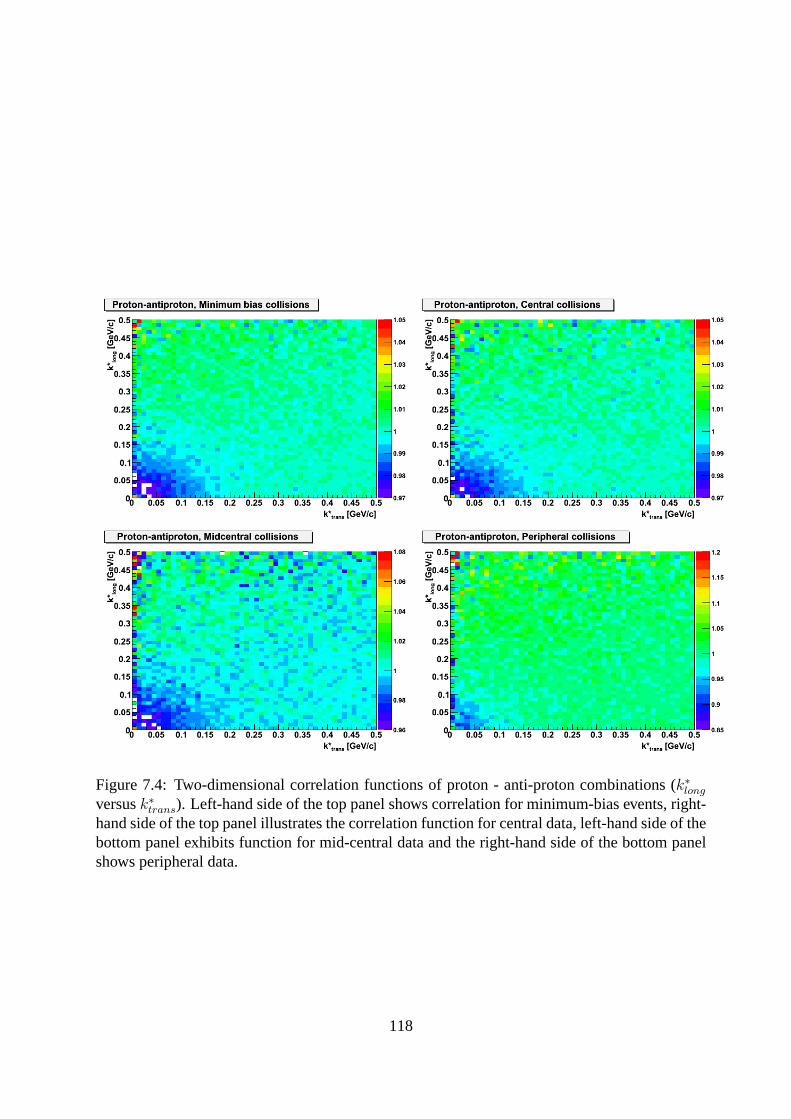
Figure 7.4: Two-dimensional correlation functions of proton - anti-proton combinations (k∗

long

versusk∗

trans). Left-hand side of the top panel shows correlation for minimum-bias events, right-hand side of the top panel illustrates the correlation function for central data, left-hand side of thebottom panel exhibits function for mid-central data and theright-hand side of the bottom panelshows peripheral data.

118

7.1.4 Two-dimensional correlation functions

As one-dimensional correlation functions are measured with a very good accuracy, two-dimensional

correlations can be also estimated. For these studies the same data collections are used. Due to

statistical limitations, the quality of such correlation functions is lower than in one-dimensional

cases. For one- and two-dimensional analysis the same statistics is considered; even if statistical

uncertainties are bigger, some properties of two-dimensional functions can be discussed. Figure

7.3 shows clearly a centrality dependency for two-proton combinations, as expected- the corre-

lation effect is stronger for less central collisions. Two-anti-proton correlations are statistically

more limited comparing to two-proton ones, thus they are notshown here. Proton - anti-proton

correlations (see Figure 7.4) have the best statistics.

Two-dimensional correlation function data is neither corrected nor fitted, experimental values of

PID numbers are not separately available for transverse andlongitudinal components of particle

momentum. These results indicate a statistical possibility for proton femtoscopy measurements

for higher than one-dimensional case. Future experiments (e.g. ALICE [92] that is being pre-

pared to operate at the LHC accelerator), where collisions of heavy-ions will occur at higher

energies that those achieved at RHIC, will provide much biggerdata collections. then, perhaps

studies of proton femtoscopy even for three-dimensional cases will be possible.

7.2 Two-proton correlations with residual correlation correc-

tions


The RCs correction introduced in Section 6.3 was applied for the results discussed in this section.

The first consequence which may be observed is the removal of significant discrepancies in

source sizes between identical and non-identical proton combinations. The results of the fits

(Table 7.3) are much closer to each other than before applying the RC corrections. Statistical

and systematic errors are listed in table as well. Systematic uncertainties are estimated from the

discrepancy between the two corrections (purity and RCs). Thestability of the fit is checked by

estimation of fitted source sizes while applying from90% to 110% of either correction for each

point of correlation function.

119

Table 7.3: Source sizes [fm] for different proton combinations and centralities; purity and RCscorrections applied; reported errors are respectively. statistical and systematic (due to purity andRCs corrections)

p − p [fm] p − p [fm] p − p [fm]

peripheral 2.79+0.11+0.05+0.06−0.11−0.05−0.06 2.81+0.13+0.08+0.14

−0.13−0.07−0.13 2.31+0.12+0.05+0.05−0.12−0.05−0.06

mid − central 4.01+0.09+0.04+0.05−0.09−0.04−0.04 4.22+0.09+0.07+0.13

−0.09−0.07−0.12 3.39+0.10+0.04+0.08−0.10−0.03−0.06

central 4.51+0.07+0.05+0.07−0.07−0.06−0.10 5.11+0.08+0.07+0.10

−0.08−0.06−0.11 4.19+0.09+0.03+0.05−0.09−0.03−0.06

7.2.2 The significance of RC correction

This section complements results shown in Section 6.3 and presents correlation functions for

all three systems and centrality bins separately; two collision energies are discussed. As it was

mentioned in Section 6.3, RCs affect proton - anti-proton system more than proton - proton one.

Figure 7.5 is composed of six panels; each of them presents correlation function before (red

points) and after (black points) applying RC correction. Forsuch identical system asp − p,

the correlation functions after taking into account the influence of RCs do not differ from those

before including an RC correlation procedure significantly.For non-identical system asp − p,

the impact of RCs is more dominant. Such dependence occurs asp − Λ RC observed inp − p is

stronger thanp−Λ RC measured withp− p (more details was discussed in Section 6.3). Due to

statistical limitationsp−p are not presented. Figure 7.6 shows results for higher collision energy-√

sNN = 200. Conclusions are similar as discussed in Section 6.3: the RCs affect non-identical

systems more. The figure complements Figure 6.7 and presentsnon-central (mid-central: first

raw, left column and peripheral: first raw, second column data) results ofp − p, non-central

(mid-central: second raw, left column and peripheral: second raw, right column data) results of

p − p and three centrality bins forp − p system (mid-central: third raw, left column, peripheral:

third raw, right column, central: fourth raw, left column).Magnitude of RC correction is not

centrality dependent, but centrality dependence ofp − Λ andp − Λ RCs measured inp − p and

p − p influence on the magnitude of RC correction.

7.2.3 All corrections applied

This section introduces fully-corrected femtoscopic measurements of proton correlations (as dis-

cussed in the previous sections, the additional correctionfor single track for resolution smearing).

The agreement between the results for identical and non-identical particle correlations for colli-

sion energy√

sNN = 200 GeV is good, however small discrepancies do remain. They fluctuate

120

Figure 7.5: Results for proton - proton (top panels) and proton - anti-proton (bottom panels)for collision energy

√sNN = 62 GeV. Correlation functions before applying RC correction (but

corrected for purity and detector resolution effects) are illustrated by red circles; correlationsafter taking into account effects of RCs are shown by black points.

121

Figure 7.6: Open symbols present correlation functions corrected for PID and fraction of primor-dial particles to be estimated to0.25; red circles show functions corrected for PID and calculatedfractions of primary particles; black points illustrate fully corrected correlation functions. Allfunctions are corrected for effect of detector resolution.Data for

√sNN = 200 GeV.

122

Figure 7.7: Results of proton femtoscopy with all corrections included: proton - proton (toppanel) anti-proton - anti-proton (middle panel) and proton- anti-proton (bottom panel). Data for√

sNN = 200 GeV.

123

with the systematic error bars- see Table 7.4. Statistical and systematic errors are listed in the

table as well. Systematic uncertainties are estimated fromthe discrepancy between three correc-

tions (purity, resolution smearing and RCs). The stability ofthe fit is checked by the estimation

of fitted source sizes while applying from90% to 110% of either correction. Results are pre-

sented in Figure 7.7. The agreement between peripheral proton - anti-proton data and the fit is

much better than before implementing a significant correction.

For lower collision energy,√

sNN = 62 GeV, correlation functions with the best fits are pre-

sented in Figure 7.8; their calculated source sizes are collected in Table 7.5. Data for lower

collision energy are statistically limited comparing to the ones for higher collision energy; thus

their agreement between experimental points and the best fits is not as good as in the case of

collision energy√

sNN = 200 GeV. For anti-proton - anti-proton system to perform such source

size calculation is almost impossible, thus not discussed here. These results indicate that all

Table 7.4: Source sizes [fm] for different proton combinations and centralities; purity, resolu-tion smearing and RCs corrections applied for collision energy

√sNN = 200; reported errors

respectively, statistical and systematic (due to purity, resolution and RCs smearing corrections)p − p [fm] p − p [fm] p − p [fm]

peripheral 2.71+0.11+0.05+0.02+0.06−0.11−0.05−0.02−0.05 2.59+0.13+0.08+0.04+0.14

−0.13−0.07−0.05−0.13 2.22+0.12+0.05+0.02+0.05−0.12−0.05−0.02−0.06

mid − central 3.82+0.09+0.04+0.02+0.05−0.09−0.04−0.02−0.04 4.02+0.09+0.07+0.04+0.13

−0.09−0.07−0.04−0.12 3.27+0.10+0.04+0.01+0.08−0.10−0.03−0.02−0.06

central 4.51+0.07+0.05+0.03+0.07−0.07−0.06−0.03−0.10 5.05+0.08+0.07+0.05+0.10

−0.08−0.06−0.04−0.11 4.08+0.09+0.03+0.02+0.05−0.09−0.03−0.01−0.06

Table 7.5: Source sizes [fm] for different proton combinations and centralities; purity, resolutionsmearing and RCs corrections applied for collision energy

√sNN = 62 GeV; reported errors

respectively, statistical and systematic (due to purity, resolution and RCs smearing corrections )p − p [fm] p − p [fm]

peripheral 2.48+0.13+0.06+0.02+0.05−0.13−0.05−0.02−0.05 2.33+0.13+0.05+0.02+0.05

−0.13−0.05−0.02−0.05

mid − central 3.23+0.12+0.06+0.02+0.09−0.12−0.05−0.02−0.06 2.72+0.13+0.05+0.02+0.04

−0.13−0.04−0.02−0.06

central 4.17+0.11+0.11+0.03+0.09−0.11−0.12−0.03−0.20 3.53+0.12+0.04+0.02+0.04

−0.12−0.03−0.01−0.05

corrections should be applied together. The RC correction isthe most essential one, it should

be performed with purity correction due to misidentification of particles. RC correction causes

all proton femtoscopic measurements to be consistent with each other. In the case of like-signs

combinations (p − p andp − p) no asymmetry in emission process between identical particles

is expected as their emission properties are identical; however, the production ofp − p pairs can

be different. On the one hand, different strong interactions between identical and non-identical

particles should not affect source sizes, as they do not concern FSI, but production mechanisms.

124

Figure 7.8: Results of proton femtoscopy with all corrections included: proton - proton (toppanel) and proton - anti-proton (bottom panel) for collision energy

√sNN = 62 GeV.

125

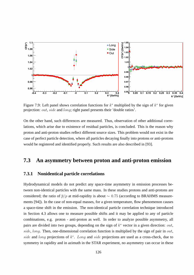
Figure 7.9: Left panel shows correlation functions fork∗ multiplied by the sign ofk∗ for givenprojection:out, side andlong; right panel presents their ’double ratios’.

On the other hand, such differences are measured. Thus, observation of other additional corre-

lations, which arise due to existence of residual particles, is concluded. This is the reason why

proton and anti-proton studies reflect different source sizes. This problem would not exist in the

case of perfect particle detection, where all particles decaying finally into protons or anti-protons

would be registered and identified properly. Such results are also described in [93].

7.3 An asymmetry between proton and anti-proton emission

7.3.1 Nonidentical particle correlations

Hydrodynamical models do not predict any space-time asymmetry in emission processes be-

tween non-identical particles with the same mass. In these studies protons and anti-protons are

considered; the ratio ofp/p at mid-rapidity is about∼ 0.75 (according to BRAHMS measure-

ments [94]). In the case of non-equal masses, for a given temperature, flow phenomenon causes

a space-time shift in the emission. The non-identical particle correlation technique introduced

in Section 4.3 allows one to measure possible shifts and it may be applied to any of particle

combinations, e.g. proton - anti-proton as well. In order toanalyze possible asymmetry, all

pairs are divided into two groups, depending on the sign ofk∗ vector in a given direction:out,

side, long. Then, one-dimensional correlation function is multiplied by the sign of pair inout,

side and long projections ofk∗. Long andside projections are used as a cross-check, due to

symmetry in rapidity and in azimuth in the STAR experiment, no asymmetry can occur in these

126

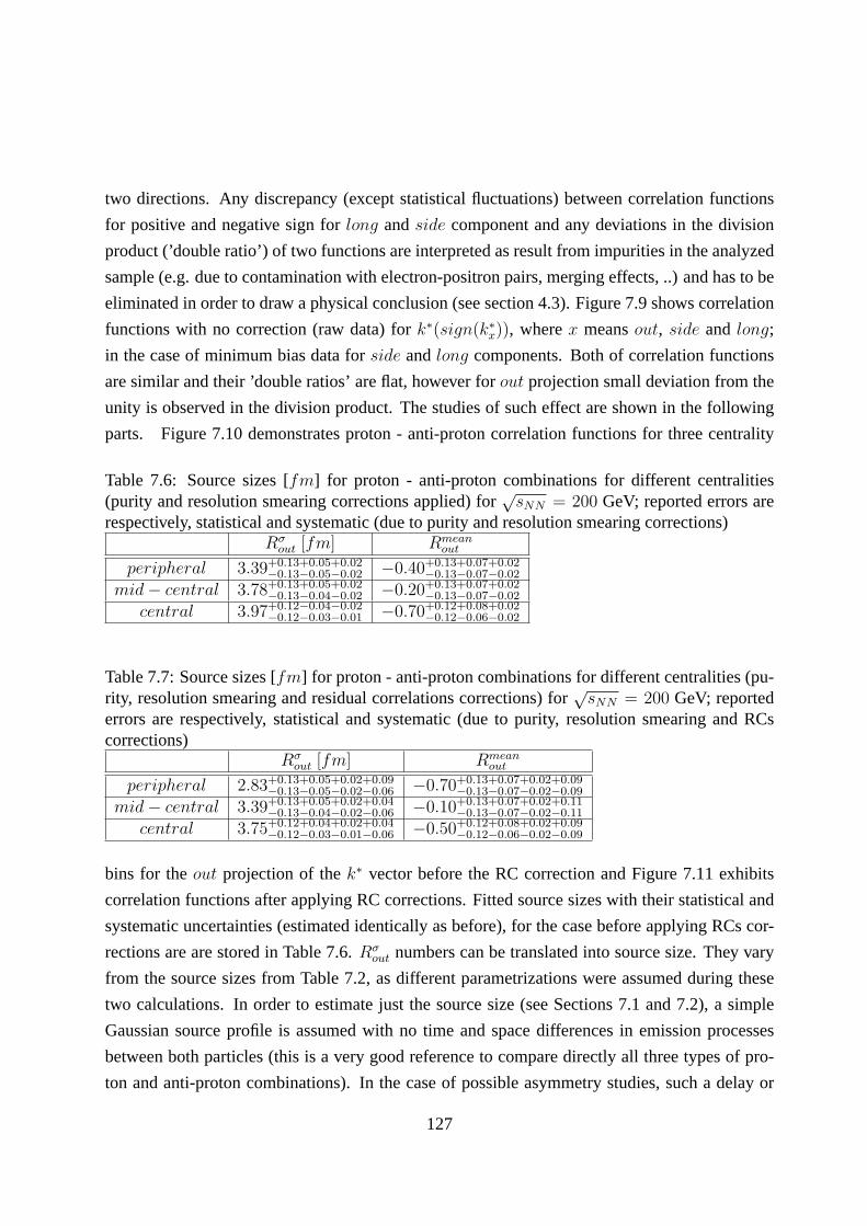
two directions. Any discrepancy (except statistical fluctuations) between correlation functions

for positive and negative sign forlong andside component and any deviations in the division

product (’double ratio’) of two functions are interpreted as result from impurities in the analyzed

sample (e.g. due to contamination with electron-positron pairs, merging effects, ..) and has to be

eliminated in order to draw a physical conclusion (see section 4.3). Figure 7.9 shows correlation

functions with no correction (raw data) fork∗(sign(k∗

x)), wherex meansout, side and long;

in the case of minimum bias data forside andlong components. Both of correlation functions

are similar and their ’double ratios’ are flat, however forout projection small deviation from the

unity is observed in the division product. The studies of such effect are shown in the following

parts. Figure 7.10 demonstrates proton - anti-proton correlation functions for three centrality

Table 7.6: Source sizes [fm] for proton - anti-proton combinations for different centralities(purity and resolution smearing corrections applied) for

√sNN = 200 GeV; reported errors are

respectively, statistical and systematic (due to purity and resolution smearing corrections)Rσ

out [fm] Rmeanout

peripheral 3.39+0.13+0.05+0.02−0.13−0.05−0.02 −0.40+0.13+0.07+0.02

−0.13−0.07−0.02

mid − central 3.78+0.13+0.05+0.02−0.13−0.04−0.02 −0.20+0.13+0.07+0.02

−0.13−0.07−0.02

central 3.97+0.12−0.04−0.02−0.12−0.03−0.01 −0.70+0.12+0.08+0.02

−0.12−0.06−0.02

Table 7.7: Source sizes [fm] for proton - anti-proton combinations for different centralities (pu-rity, resolution smearing and residual correlations corrections) for

√sNN = 200 GeV; reported

errors are respectively, statistical and systematic (due to purity, resolution smearing and RCscorrections)

Rσout [fm] Rmean

out

peripheral 2.83+0.13+0.05+0.02+0.09−0.13−0.05−0.02−0.06 −0.70+0.13+0.07+0.02+0.09

−0.13−0.07−0.02−0.09

mid − central 3.39+0.13+0.05+0.02+0.04−0.13−0.04−0.02−0.06 −0.10+0.13+0.07+0.02+0.11

−0.13−0.07−0.02−0.11

central 3.75+0.12+0.04+0.02+0.04−0.12−0.03−0.01−0.06 −0.50+0.12+0.08+0.02+0.09

−0.12−0.06−0.02−0.09

bins for theout projection of thek∗ vector before the RC correction and Figure 7.11 exhibits

correlation functions after applying RC corrections. Fitted source sizes with their statistical and

systematic uncertainties (estimated identically as before), for the case before applying RCs cor-

rections are are stored in Table 7.6.Rσout numbers can be translated into source size. They vary

from the source sizes from Table 7.2, as different parametrizations were assumed during these

two calculations. In order to estimate just the source size (see Sections 7.1 and 7.2), a simple

Gaussian source profile is assumed with no time and space differences in emission processes

between both particles (this is a very good reference to compare directly all three types of pro-

ton and anti-proton combinations). In the case of possible asymmetry studies, such a delay or

127

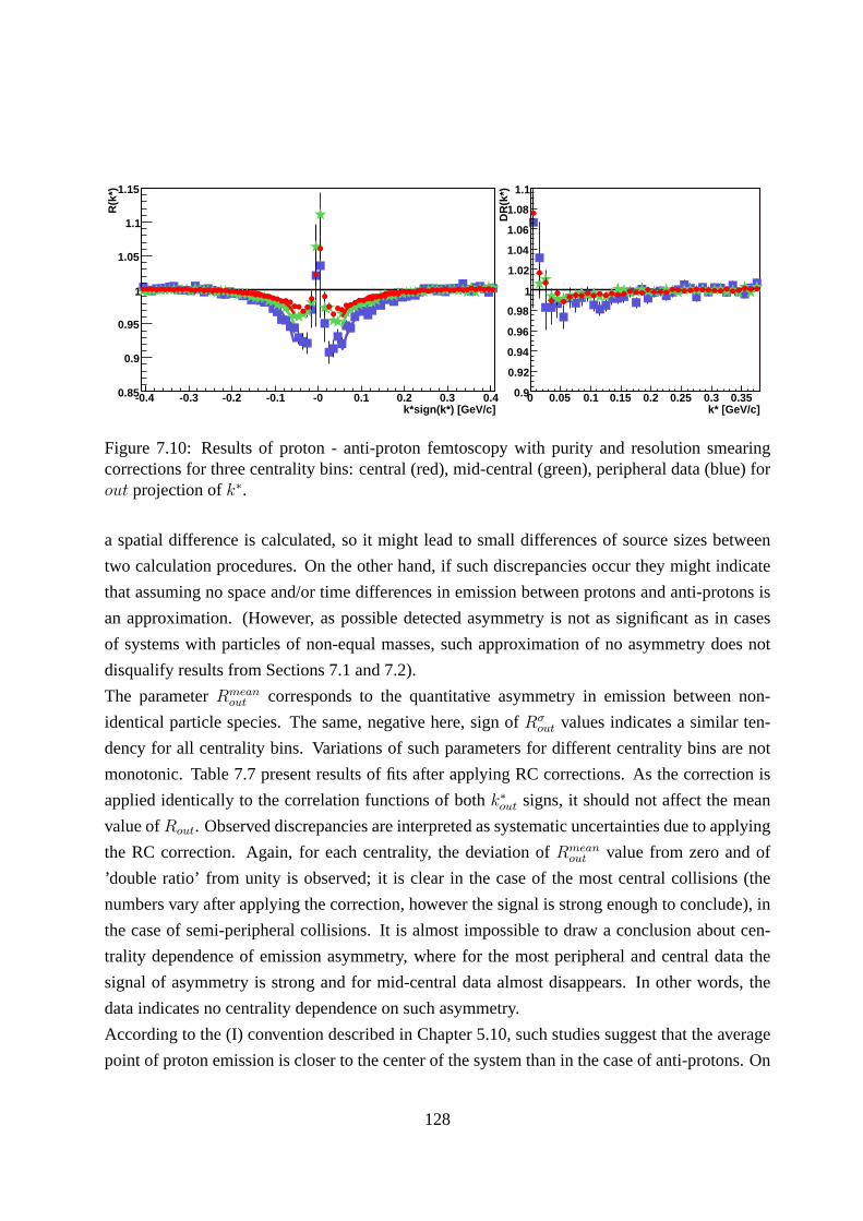
k*sign(k*) [GeV/c]-0.4 -0.3 -0.2 -0.1 -0 0.1 0.2 0.3 0.4

R(k

*)

0.85

0.9

0.95

1

1.05

1.1

1.15

k* [GeV/c]0 0.05 0.1 0.15 0.2 0.25 0.3 0.35

DR

(k*)

0.9

0.92

0.94

0.96

0.98

1

1.02

1.04

1.06

1.08

1.1

Figure 7.10: Results of proton - anti-proton femtoscopy withpurity and resolution smearingcorrections for three centrality bins: central (red), mid-central (green), peripheral data (blue) forout projection ofk∗.

a spatial difference is calculated, so it might lead to smalldifferences of source sizes between

two calculation procedures. On the other hand, if such discrepancies occur they might indicate

that assuming no space and/or time differences in emission between protons and anti-protons is

an approximation. (However, as possible detected asymmetry is not as significant as in cases

of systems with particles of non-equal masses, such approximation of no asymmetry does not

disqualify results from Sections 7.1 and 7.2).

The parameterRmeanout corresponds to the quantitative asymmetry in emission between non-

identical particle species. The same, negative here, sign of Rσout values indicates a similar ten-

dency for all centrality bins. Variations of such parameters for different centrality bins are not

monotonic. Table 7.7 present results of fits after applying RCcorrections. As the correction is

applied identically to the correlation functions of bothk∗

out signs, it should not affect the mean

value ofRout. Observed discrepancies are interpreted as systematic uncertainties due to applying

the RC correction. Again, for each centrality, the deviationof Rmeanout value from zero and of

’double ratio’ from unity is observed; it is clear in the caseof the most central collisions (the

numbers vary after applying the correction, however the signal is strong enough to conclude), in

the case of semi-peripheral collisions. It is almost impossible to draw a conclusion about cen-

trality dependence of emission asymmetry, where for the most peripheral and central data the

signal of asymmetry is strong and for mid-central data almost disappears. In other words, the

data indicates no centrality dependence on such asymmetry.

According to the (I) convention described in Chapter 5.10, such studies suggest that the average

point of proton emission is closer to the center of the systemthan in the case of anti-protons. On

128

R(k

*)

0.75

0.8

0.85

0.9

0.95

1

1.05

1.1

1.1530-80%

R(k

*)

0.75

0.8

0.85

0.9

0.95

1

1.05

1.1

1.1510-30%

) [GeV]out

k*sign(k*-0.4 -0.3 -0.2 -0.1 -0 0.1 0.2 0.3 0.4

R(k

*)

0.75

0.8

0.85

0.9

0.95

1

1.05

1.1

1.15

0-10%

DR

(k*)

0.85

0.9

0.95

1

1.05

1.1

1.15

DR

(k*)

0.85

0.9

0.95

1

1.05

1.1

1.15

k* [GeV]0 0.05 0.1 0.15 0.2 0.25 0.3 0.35

DR

(k*)

0.85

0.9

0.95

1

1.05

1.1

1.15

Figure 7.11: Results of proton - anti-proton femtoscopy withall corrections applied.

129

Figure 7.12: Results of proton femtoscopy with all corrections applied for minimum-bias colli-sions for three different projections ofk∗.

the other hand, protons are also considered as emitted later(on average) than anti-protons.

In such case when proton is faster (correlation function fork∗

out > 0) it catches up to the slower

anti-proton, so they stay close to each other longer, their effective interaction time is longer, hence

the correlation effect is stronger. When proton is slower (correlation function fork∗

out < 0), the

faster anti-proton flies away fast, the time they spend closeto each other is short, hence the ef-

fective interaction time is short and the correlation effect is smaller.

Figure 7.12 presents results fully corrected (RC correctionincluded as well) for minimum-bias

collisions with the respect to the sign of each component:out, side andlong. Deviation from

unity for theout component is clearly visible, while ’double ratio’ for two other ones remains

almost flat. In order to try to check whether the asymmetry (and in which centrality) occurs, the

new technique of spherical decomposition is studied.

7.3.2 Spherical Harmonics decomposition

Three-dimensional correlation function can be decomposedinto three components [95, 96], as

shown in Figure 7.13. The spherical coordinatesθ, φ,Q are related to the Cartesian coordinates

as:

Qo = Qsinθcosφ (7.1)

QS = Qsinθsinφ (7.2)

QL = Qcosθ (7.3)

130

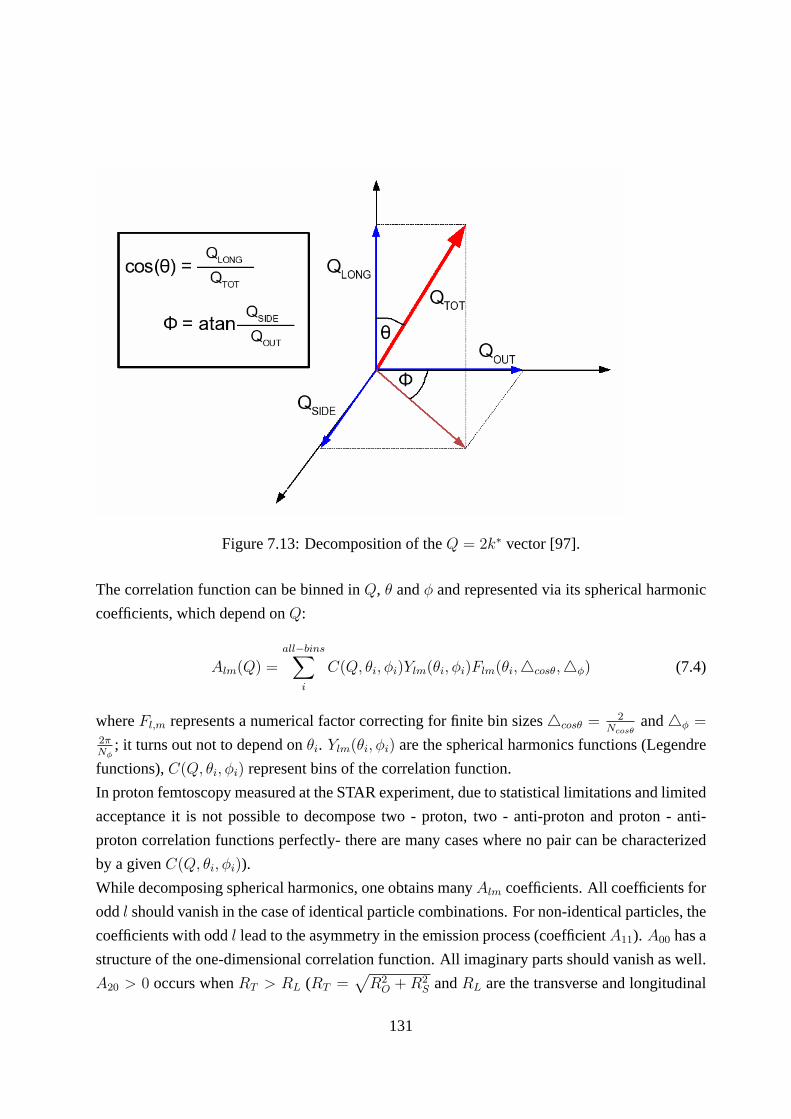
Figure 7.13: Decomposition of theQ = 2k∗ vector [97].

The correlation function can be binned inQ, θ andφ and represented via its spherical harmonic

coefficients, which depend onQ:

Alm(Q) =all−bins∑

i

C(Q, θi, φi)Ylm(θi, φi)Flm(θi,cosθ,φ) (7.4)

whereFl,m represents a numerical factor correcting for finite bin sizescosθ = 2Ncosθ

andφ =2πNφ

; it turns out not to depend onθi. Ylm(θi, φi) are the spherical harmonics functions (Legendre

functions),C(Q, θi, φi) represent bins of the correlation function.

In proton femtoscopy measured at the STAR experiment, due tostatistical limitations and limited

acceptance it is not possible to decompose two - proton, two -anti-proton and proton - anti-

proton correlation functions perfectly- there are many cases where no pair can be characterized

by a givenC(Q, θi, φi)).

While decomposing spherical harmonics, one obtains manyAlm coefficients. All coefficients for

oddl should vanish in the case of identical particle combinations. For non-identical particles, the

coefficients with oddl lead to the asymmetry in the emission process (coefficientA11). A00 has a

structure of the one-dimensional correlation function. All imaginary parts should vanish as well.

A20 > 0 occurs whenRT > RL (RT =√

R2O + R2

S andRL are the transverse and longitudinal

131

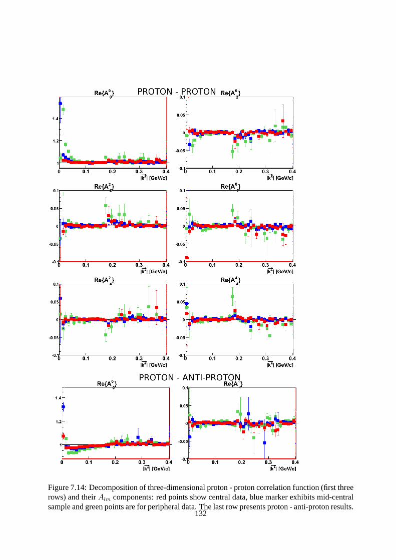
Figure 7.14: Decomposition of three-dimensional proton - proton correlation function (first threerows) and theirAlm components: red points show central data, blue marker exhibits mid-centralsample and green points are for peripheral data. The last rowpresents proton - anti-proton results.

132

components of radii of source respectively),A20 < 0 otherwise. A22 > 0 tells if Ro < Rs,

A22 < 0 in the opposite scenario. As shown in Figure 7.14 (proton - proton), the source seems

to be spherical. In the case on non-identical proton - anti-proton systems (Figure 7.14, bottom

part), the most interesting coefficient isA11, which especially for central collisions seems to

deviate from zero value. For other centralities, statistical limitations occurs. For each system,

centrality dependence is reflected inA00 coefficients, which claims propriety of decomposition

technique. It is clear that for proton femtoscopy it is very difficult to conclude about source

properties basing on spherical harmonics decomposition, due to statistical limitations. However,

the results on non-identical particle correlation technique have not been discarded.

Application of the RC correction would not change conclusions as the correction would be iden-

tically done on each direction (the same scaling factor within the samek∗). On the other hand,

the RC correction would provide an additional source of uncertainty, so drawing any conclusions

would be much more difficult than in the case on non-correcteddata.

133

Chapter 8

Discussion

8.1 Importance of residual correlation corrections

Fully corrected correlation functions forAu + Au collisions at√

sNN = 200 GeV for differ-

ent centrality bins are shown in Figure 7.7. For lower collision energy-√

sNN = 62 GeV such

corrected correlations (proton - proton and proton - anti-proton systems) are presented in Figure

7.8. For all systems the correlation effect decreases with increasing centrality. The extracted

Gaussian radii with their statistical and systematic uncertainties are given in Section 7.2 in the

Tables 7.4 and 7.5, for√

sNN = 200 GeV and√

sNN = 62 GeV respectively. The approxi-

mate consistence for different pair combinations, for all energies and centrality selections, gives

confidence in the stability of our results. Comparing resultsfor two collision energies, they are

consistent within error-bars, however in the most systems and centralities, the radii deduced for

lower collision energy are slightly lower, which is interpreted as a consequence of lower particle

multiplicities registered in such collisions (more in Section 8.2). Results not corrected for RCs

are shown in Section 7.1. Radii for identical particles vary from non-identical ones as additional

correlations measured withp − p, p − p andp − p were not taken into account. Neglecting the

presence of residual sources of correlations may significantly falsify physical conclusions, thus

correct source sizes and their agreement for identical and non-identical protons and anti-protons

combinations would not be possible to deduce if the RC correction had not been applied.

134

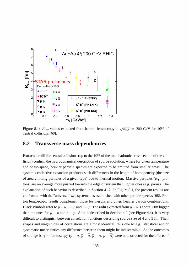
Figure 8.1:Rinv values extracted from hadron femtoscopy at√

sNN = 200 GeV for 10% ofcentral collisions [68].

8.2 Transverse mass dependencies

Extracted radii for central collisions (up to the10% of the total hadronic cross-section of the col-

lision) confirm the hydrodynamical description of source evolution, where for given temperature

and phase-space, heavier particle species are expected to be emitted from smaller areas. The

system’s collective expansion produces such differences in the length of homogeneity (the size

of area emitting particles of a given type) due to thermal motion. Massive particles (e.g. pro-

tons) are on average more pushed towards the edge of system than lighter ones (e.g. pions). The

explanation of such behavior is described in Section 4.12. In Figure 8.1, the present results are

confronted with the "universal"mT systematics established with other particle species [68].Pro-

ton femtoscopic results complement those for mesons and other, heavier baryon combinations.

Black symbols refer top−p, p−p andp−p. The radii extracted fromp−p is about 1 fm bigger

than the ones forp − p andp − p. As it is described in Section 4.9 (see Figure 4.4), it is very

difficult to distinguish between correlation functions describing source size of 4 and 5 fm. Their

shapes and magnitudes of correlations are almost identical, thus due to e.g. statistical and/or

systematic uncertainties any difference between them might be indiscernible. As the outcomes

of strange baryon femtoscopy (p − Λ, p − Λ, p − Λ, p − Λ) were not corrected for the effects of

135

Figure 8.2:(dNch/dη)1/3 scaling of source sizes from proton femtoscopy at√

sNN = 62 GeVand

√sNN = 200 GeV

RCs, the results of correlation forp− Λ andp− Λ are expected to be affected stronger than two

other ones by RCs, thus observables indicated by green points are more reliable. In general, the

results of proton femtoscopy agree with the other STAR measurement more.

8.3 Multiplicity dependencies

Another experimental result is the nature of the(dNch/dη)1/3 scaling (Nch- number of charge

particles) of HBT radii, seen in pion interferometry [68]. Itis observed also in proton femtoscopy.

Studying such relations is motivated by relations of(dNch/dη)1/3 dependencies with the final

state geometry through particle density at freeze-out. Figure 8.2 presents such scaling forRinv

source sizes extracted fromp − p, p − p andp − p at√

sNN = 62 GeV and√

sNN = 200 GeV

energies. Errors shown are both statistical and systematic. Comparing to pion measurements,

proton ones are smaller by the order of∼ 1 fm. Discrepancies between three systems are shown,

however results agree with error-bars. Source sizes monotonically increase with(dNch/dη)1/3.

Radii fluctuate due to statistical limitations. Such figures for identical pion observables present

a linear dependence of(dNch/dη)1/3 (multiplicity, which is distinguished via collision central-

136

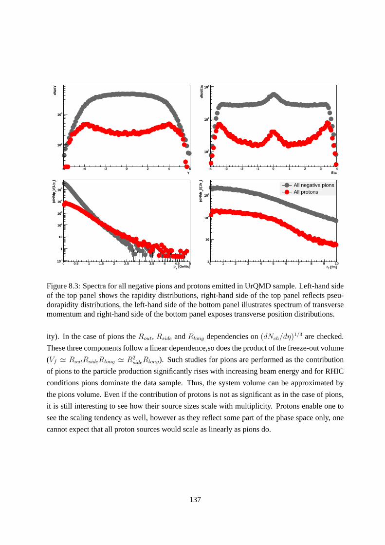
Y-6 -4 -2 0 2 4 6

dN

/dY

210

310

Eta-4 -3 -2 -1 0 1 2 3 4

dN

/dE

ta

210

310

410

[GeV/c]T

p0 0.5 1 1.5 2 2.5 3 3.5 4 4.5 5

)T

)/(1

/pT

(dN

/dp

-110

1

10

210

310

410

510

[fm]Tr0 1 2 3 4 5 6 7 8 9 10

)T

)/(1

/rT

(dN

/dr

1

10

210

310

All negative pionsAll protons

Figure 8.3: Spectra for all negative pions and protons emitted in UrQMD sample. Left-hand sideof the top panel shows the rapidity distributions, right-hand side of the top panel reflects pseu-dorapidity distributions, the left-hand side of the bottompanel illustrates spectrum of transversemomentum and right-hand side of the bottom panel exposes transverse position distributions.

ity). In the case of pions theRout, Rside andRlong dependencies on(dNch/dη)1/3 are checked.

These three components follow a linear dependence,so does the product of the freeze-out volume

(Vf ≃ RoutRsideRlong ≃ R2sideRlong). Such studies for pions are performed as the contribution

of pions to the particle production significantly rises withincreasing beam energy and for RHIC

conditions pions dominate the data sample. Thus, the systemvolume can be approximated by

the pions volume. Even if the contribution of protons is not as significant as in the case of pions,

it is still interesting to see how their source sizes scale with multiplicity. Protons enable one to

see the scaling tendency as well, however as they reflect somepart of the phase space only, one

cannot expect that all proton sources would scale as linearly as pions do.

137

8.4 Comparison with model predictions

This subsection presents the results of simulations with two theoretical models: UrQMD and

EPOS. First, simple one-particle distributions are discussed: rapidity, pseudorapidity, transverse

momentum and freeze-out coordinates. Then, two-particle separation distributions are shown

(see Appendix 3 for details). Many systems composed of various particle combinations are

checked and compared to each other, but only distributions of protons and anti-protons are shown

here; non-identical combinations are also discussed (pions and kaons). The possibility to detect

asymmetry in the emission process is checked on experimentally known cases (like and un-like

signs combinations of pions and kaons). These studies are treated as a base for deducing possible

asymmetry in emission between protons and their antiparticles.

8.4.1 UrQMD

Single-particle distributions

Single-particle distributions allow one to take a look intoparticle production mechanisms. The

UrQMD model was discussed in Section 3.1. Data has been gathered for Au + Au collisions

at√

sNN = 200 GeV. In order to see how the production mechanisms look like,the following

distributions are calculated: rapidity, pseudorapidity,transverse momentum:pT =√

p2x + p2

y

and transverse freeze-out position:rT =√

r2x + r2

y. Seen in the Figure 8.3 increased numbers

of protons at higher rapidity and pseudorapidity intervalsare a result of taking nuclear remnants

into account. Higher multiplicities of pions are generated. Due to higher proton mass, more

protons with higher transverse momentum are observed as compared to pions. The last plot of

Figure 8.3 presents the distribution ofrT . Figure 8.4 shows ratios of particle productions ver-

sus rapidity. The ratio of negative to positive pions remains flat through of the rapidity interval,

showing that similar amount of negative and positive pions are produced (the production ofπ−

mesons is slightly increased in higher rapidity ranges). The production of kaons is not identical

for positive and negative particle species. In mid-rapidity interval (up to|y| = 2) production of

K+ andK− hadrons is similar; for higher rapidity values, productionof positive kaons domi-

nates. For protons, even for mid-rapidity (|y| < 1), twice as many protons are produced as their

anti-particles. For the highest of ranges of rapidities shown here, the production of anti-protons

is highly decreased. Comparing to RHIC measurements (BRAHMS [94]), pion production in

UrQMD is similar to measured in the experiment and for mid-peripheral rapidities kaon pro-

duction looks comparable as well, however for the highest rapidities in UrQMD production of

138

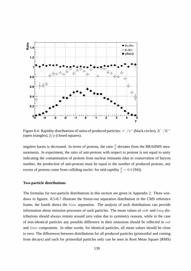
Figure 8.4: Rapidity distributions of ratios of produced particles:π−/π+ (black circles),K−/K+

(open triangles),p/p (closed squares).

negative kaons is decreased. In terms of protons, the ratiopp

deviates from the BRAHMS mea-

surements. In experiment, the ratio of anti-protons with respect to protons is not equal to unity

indicating the contamination of protons from nuclear remnants (due to conservation of baryon

number, the production of anti-protons must be equal to the number of produced protons, any

excess of protons come from colliding nuclei- for mid-rapidity pp∼ 0.8 [94]).

Two-particle distributions

The formulas for two-particle distributions in this section are given in Appendix 2. Three win-

dows in figures: 8.5-8.7 illustrate the freeze-out separation distribution in the CMS reference

frame; the fourth shows thetime separation. The analysis of such distributions can provide

information about emission processes of such particles. The mean values ofside andlong dis-

tributions should always remain around zero value due to symmetry reasons, while in the case

of non-identical particles any possible difference in their emissions should be reflected inout

andtime components. In other words, for identical particles, all mean values should be close

to zero. The differences between distributions for all produced particles (primordial and coming

from decays) and such for primordial particles only can be seen in Root Mean Square (RMS)

139

[fm]-40 -30 -20 -10 0 10 20 30 40

dN

/dr

ou

t

310

410

ALL p-p PRIMARY p-p

[fm]-40 -30 -20 -10 0 10 20 30 40

dN

/dr

sid

e

310

410

[fm]-40 -30 -20 -10 0 10 20 30 40

dN

/dr

lon

g

310

410

[fm]-40 -30 -20 -10 0 10 20 30 40

dN

/dr

tim

e

410

Figure 8.5: Two-proton separation distributions for all particles (gray points) and primordial only(red points) in CMS reference. Top-left panel presents separation forout component, top-rightpanel illustratesside component separation, bottom-left panel reflects separation distribution forlong component and bottom-right panel exhibits time separation.

140

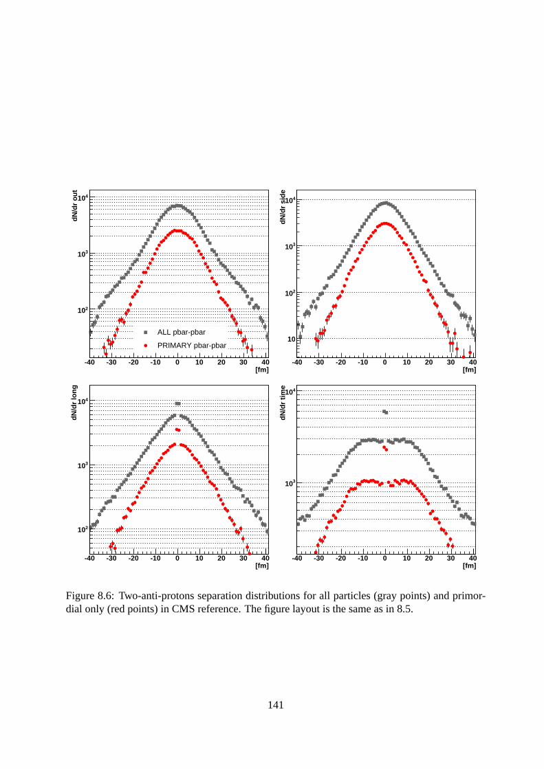
[fm]-40 -30 -20 -10 0 10 20 30 40

dN

/dr

ou

t

210

310

410

ALL pbar-pbar

PRIMARY pbar-pbar

[fm]-40 -30 -20 -10 0 10 20 30 40

dN

/dr

sid

e

10

210

310

410

[fm]-40 -30 -20 -10 0 10 20 30 40

dN

/dr

lon

g

210

310

410

[fm]-40 -30 -20 -10 0 10 20 30 40

dN

/dr

tim

e

310

410

Figure 8.6: Two-anti-protons separation distributions for all particles (gray points) and primor-dial only (red points) in CMS reference. The figure layout is the same as in 8.5.

141

values, where the width of distributions can be transformedto the source size emitting particles.

By primordial (or primary) proton is meant such particle, which does not come from the weak

decay ofΛ or Σ+ hyperons. Primordial (or primary) anti-proton is such particle, which does not

come from weak decay ofΛ or Σ+. Primordial particles come from a smaller area than non-

primary particles which might come from much bigger sources. Distributions of all particles

are always plotted in gray and those for primordial particlespecies- in red. Figure 8.5 presents

two-proton separation distributions (the peaks inlong andtime distribution appears as a conse-

quence of taking into account particles lying very close to the z axis in the laboratory frame),

Figure 8.6 illustrates two-anti-proton distributions; see Tables 9.10 and 9.11; comparing to two-

proton distributions, the scale on the vertical axises are different) and Figure 8.7 presents proton

- anti-proton distributions (as a first particle proton is denoted, as a second one- anti-proton).

Especially important are those for primordial particles, where the separation distributions forout

direction andtime remain away from zero, indicating some asymmetry in the emission process

(see Table 8.1). For identical particle combinations all values remain close to zero, except the

few containing remnants from nuclear matter which might contaminate the analyzed sample (see

Figure 8.5 and 8.6). Each distribution does not represent Gaussian shape (which is indicated by

the general shape of each distribution- they have ’non-gaussian’ tails observed in the logarithmic

scale, so a Gaussian can be fitted to the central parts ofout andside distributions only), as the

model generates tails which cannot be parametrized in this way.

Correlations

As the UrQMD model gives momenta and freeze-out coordinates, it is possible to calculate corre-

lation functions for many particle combinations as long as generated statistics enables estimation

of the shape of correlation. In Figure 8.8 correlation functions for identical particles are pre-

sented: pion-pion correlation functions, taking into account both QS and Coulomb interactions

for all positive pions (gray points) and for primordial particles only (red points). Obviously, the

correlation function calculated for primary particles only is stronger and leads to smaller source

sizes than in the other cases. The same conclusion comes fromproton-proton correlations: gray

points illustrate correlation of all protons and red pointscorrespond to the primordial protons

only (not taking into account the remnants of colliding nuclei). In order to increase statistics, the

correlation functions for anti-proton - anti-proton are calculated as well and then their numera-

tors and denominators respectively were added in order to obtain correlation functions. Besides

identical particle combinations, the non-identical ones are considered as well. In the bottom

panel of Figure 8.9, correlations for like-signs combinations of pions and kaons are shown. All

142

[fm]-40 -30 -20 -10 0 10 20 30 40

dN

/dr

ou

t

210

310

410

ALL p-pbar

PRIMARY p-pbar

[fm]-40 -30 -20 -10 0 10 20 30 40

dN

/dr

sid

e310

410

[fm]-40 -30 -20 -10 0 10 20 30 40

dN

/dr

lon

g

310

410

[fm]-40 -30 -20 -10 0 10 20 30 40

dN

/dr

tim

e

310

410

Figure 8.7: Proton-anti-proton separation distributionsfor all particles (gray points) and primor-dial only (red points) in CMS reference. The figure layout is the same as in 8.5.

143

k* [GeV/c]0 0.02 0.04 0.06 0.08 0.1

CF

(k*)

0

0.2

0.4

0.6

0.8

1

1.2

1.4

1.6

1.8

2

--Pi-ALL Pi--Pi-PRIMARY Pi

k* [GeV/c]0 0.02 0.04 0.06 0.08 0.1

CF

(k*)

0

0.2

0.4

0.6

0.8

1

1.2

1.4

1.6

1.8

2ALL P-P

PRIMARY P-P

Figure 8.8: Identical two-particle correlations (two-pion and two-proton) from UrQMD.

pairs were divided into two groups (following the same rulesof the STAR Collaboration, see

Section 5.12). Dividing the correlation for positive sign of k∗

out by the one for negative sign, it is

possible to detect the differences in the emission, depending on the deviations of ‘double ratio’

from unity (see the right panel of Figure 8.10 for like-sign combination). The top panel of Figure

8.9 and the left panel of Figure 8.10 present results for unlike-signs. The ’double ratio’ for the

same signs of particles goes below unity and for opposite signs it rises above unity exactly as

observed at STAR, indicating than in the model pions are in average emitted from bigger area

(or earlier) than kaons (according to the flow prediction). These correlations are obtained for

minimum-bias collisions, where impact parameters indicating the collision centrality is in the

wide rangeb ∈ [0; 15] fm; therefore the magnitude of detected asymmetry cannot becompared

directly to the STAR data.

Figure 8.11 shows proton - anti-proton correlation functions. The correlation effect clearly

indicates annihilation of protons and their anti-particles. The first plot in Figure 8.11 shows

correlation function with respect to the sign ofk∗

out, the last plot illustrates one dimensional cor-

relation function; for smallk∗ values (close to0 GeV/c), an attraction due to Coulomb forces

can be noticed, then an annihilation channel due to strong interactions is present. Two of the

’double ratios’ indicate small deviation from the zero value (the tendency is illustrated below

unity), which indicates that on average stronger correlation occurs fork∗

out > 0. These model

predictions are consistent with experimental results. Thesame convection (described in Section

144

Figure 8.9: Pion-kaon (like signs in bottom panel and un-like signs at top panel) correlation func-tion. Grey marker shows correlation functions calculated for all particles, red marker indicatescorrelation functions for primordial particles only

145

Figure 8.10: Pion-kaon (like sign in right panel and un-likesigns at left panel) double ratios. Greymarker shows ’double ratios’ calculated for all particles,red marker indicates ’double ratios’ forprimordial particles only

146

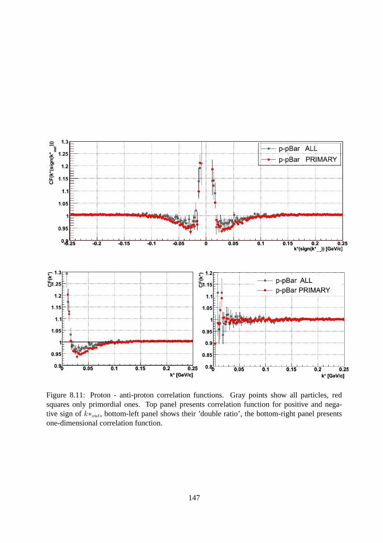
Figure 8.11: Proton - anti-proton correlation functions. Gray points show all particles, redsquares only primordial ones. Top panel presents correlation function for positive and nega-tive sign ofk∗out, bottom-left panel shows their ’double ratio’, the bottom-right panel presentsone-dimensional correlation function.

147

4.10) as in data analysis is used, so the fact that ’double ratio’ is below unity for smallerk∗values indicate that in model in average protons are emittedfrom bigger area and/or earlier than

anti-protons.

Asymmetry discussion

As it was mentioned in the previous sections, the asymmetry in emission mechanisms can be

detected in non-identical particle combinations. Figure 8.12 shows two-particle separation dis-

tributions in the CMS reference, same for primordial protonsand anti-protons only, for 3 classes

of centrality: central collisions (up to 10% of the total hadronic cross section of the collision),

(10-30)% and (30-80)%. The plots and corresponding tables (Table 8.1 for Figure 8.12 and Table

9.12 for Figure 8.7) show that the deviation of the mean valueof Rout distributions from zero in-

dicates possible spatial asymmetry of emission between protons and anti-protons. There is also

an asymmetry in time indicated by time distributions. All these deviations monotonically rise

from central to peripheral collisions: for central collisions the deviation ofRout separation dis-

tribution from zero value is around0.7 fm, for mid-central-∼ 0.9 fm for peripheral data-∼ 1.2

fm. Such behavior indicates influence of final-state rescattering; non-central collisions seem to

be affected more, thus stronger effect in two-particle separation distributions. The mean values

and RMS are stored in Table 8.1 (together with results for the EPOS model). Tables 9.8 and 9.9

present the values of separation distributions from pion-kaon distributions (together with results

for EPOS).

8.4.2 EPOS

Single-particle distributions

The same single-particle distributions are presented for the EPOS model. Data gathered for

Au+Au collisions at√

sNN = 200 GeV, same as for UrQMD sample, are shown in Section 8.4.1.

Figure 8.13 shows rapidity, pseudorapidity, transverse momentum and position spectra. Here,

mid-rapidity and mid-pseudorapidity (up to|y| = 2 and|η| = 2) pion and proton distributions

are constant, for the other ranges of rapidity and pseudorapidity (|y| > 2 and|η| > 2) they are

naturally decreasing. Concerning momentum spectra, as pions have smaller mass, they populate

mainly lower momentum intervals. The last plot in Figure 8.13 indicatesrT . Figure 8.14 shows

rapidity distributions of particle ratios. For mid-rapidity (|y| < 2), ratios: π−

π+ and K−

K+ are flat.

148

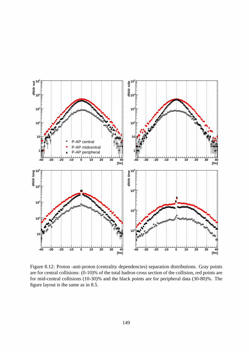
[fm]-40 -30 -20 -10 0 10 20 30 40

dN

/dr

ou

t

1

10

210

310

410

510

P-AP centralP-AP midcentralP-AP peripheral

[fm]-40 -30 -20 -10 0 10 20 30 40

dN

/dr

sid

e

1

10

210

310

410

510

[fm]-40 -30 -20 -10 0 10 20 30 40

dN

/dr

lon

g

10

210

310

410

510

[fm]-40 -30 -20 -10 0 10 20 30 40

dN

/dr

tim

e

210

310

410

510

Figure 8.12: Proton -anti-proton (centrality dependencies) separation distributions. Gray pointsare for central collisions: (0-10)% of the total hadron cross section of the collision, red points arefor mid-central collisions (10-30)% and the black points are for peripheral data (30-80)%. Thefigure layout is the same as in 8.5.

149

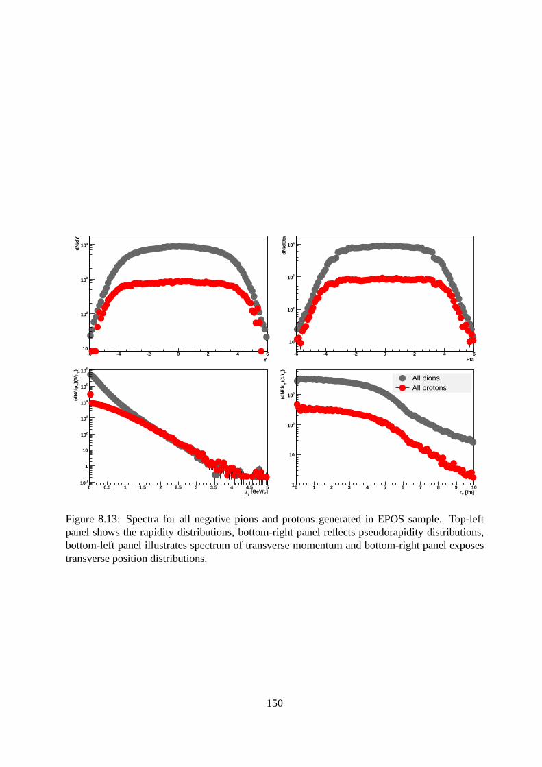
Y-6 -4 -2 0 2 4 6

dN

/dY

10

210

310

410

Eta-6 -4 -2 0 2 4 6

dN

/dE

ta

10

210

310

410

[GeV/c]T

p0 0.5 1 1.5 2 2.5 3 3.5 4 4.5 5

)T

)(1/

pT

(dN

/dp

-110

1

10

210

310

410

510

610

[fm]Tr0 1 2 3 4 5 6 7 8 9 10

)T

)(1/

rT

(dN

/dr

1

10

210

310

All pionsAll protons

Figure 8.13: Spectra for all negative pions and protons generated in EPOS sample. Top-leftpanel shows the rapidity distributions, bottom-right panel reflects pseudorapidity distributions,bottom-left panel illustrates spectrum of transverse momentum and bottom-right panel exposestransverse position distributions.

150

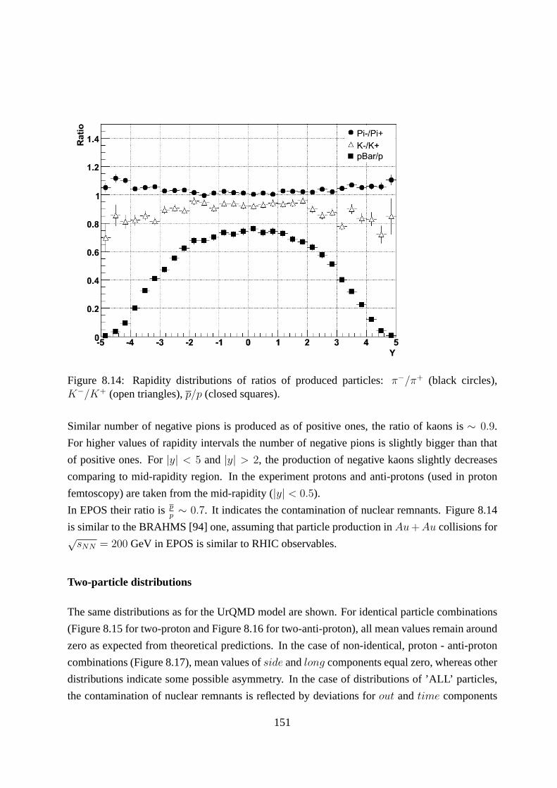
Figure 8.14: Rapidity distributions of ratios of produced particles: π−/π+ (black circles),K−/K+ (open triangles),p/p (closed squares).

Similar number of negative pions is produced as of positive ones, the ratio of kaons is∼ 0.9.

For higher values of rapidity intervals the number of negative pions is slightly bigger than that

of positive ones. For|y| < 5 and |y| > 2, the production of negative kaons slightly decreases

comparing to mid-rapidity region. In the experiment protons and anti-protons (used in proton

femtoscopy) are taken from the mid-rapidity (|y| < 0.5).

In EPOS their ratio ispp∼ 0.7. It indicates the contamination of nuclear remnants. Figure 8.14

is similar to the BRAHMS [94] one, assuming that particle production inAu + Au collisions for√

sNN = 200 GeV in EPOS is similar to RHIC observables.

Two-particle distributions

The same distributions as for the UrQMD model are shown. For identical particle combinations

(Figure 8.15 for two-proton and Figure 8.16 for two-anti-proton), all mean values remain around

zero as expected from theoretical predictions. In the case of non-identical, proton - anti-proton

combinations (Figure 8.17), mean values ofside andlong components equal zero, whereas other

distributions indicate some possible asymmetry. In the case of distributions of ’ALL’ particles,

the contamination of nuclear remnants is reflected by deviations forout andtime components

151

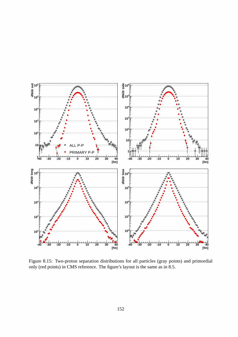
[fm]-40 -30 -20 -10 0 10 20 30 40

dN

/dr

ou

t

1

10

210

310

410

510

610

ALL P-P

PRIMARY P-P

[fm]-40 -30 -20 -10 0 10 20 30 40

dN

/dr

sid

e

1

10

210

310

410

510

610

[fm]-40 -30 -20 -10 0 10 20 30 40

dN

/dr

lon

g

210

310

410

510

610

[fm]-40 -30 -20 -10 0 10 20 30 40

dN

/dr

tim

e

210

310

410

510

610

Figure 8.15: Two-proton separation distributions for all particles (gray points) and primordialonly (red points) in CMS reference. The figure’s layout is the same as in 8.5.

152

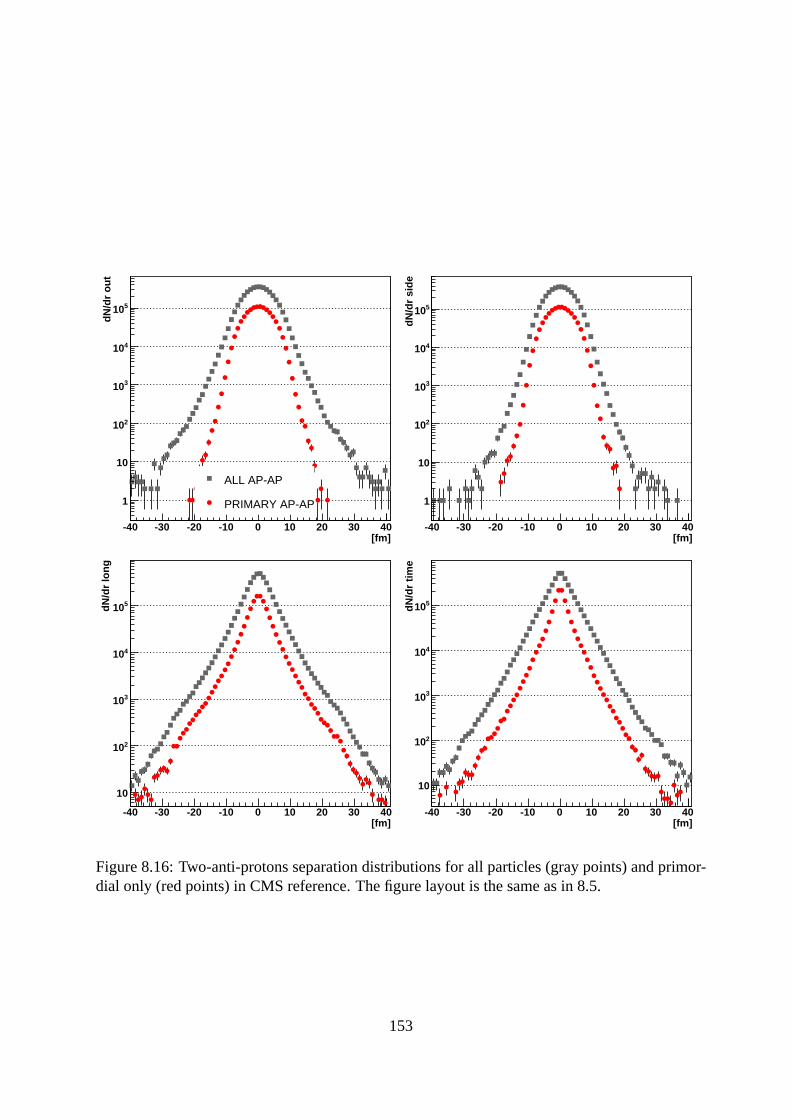
[fm]-40 -30 -20 -10 0 10 20 30 40

dN

/dr

ou

t

1

10

210

310

410

510

ALL AP-AP

PRIMARY AP-AP

[fm]-40 -30 -20 -10 0 10 20 30 40

dN

/dr

sid

e

1

10

210

310

410

510

[fm]-40 -30 -20 -10 0 10 20 30 40

dN

/dr

lon

g

10

210

310

410

510

[fm]-40 -30 -20 -10 0 10 20 30 40

dN

/dr

tim

e

10

210

310

410

510

Figure 8.16: Two-anti-protons separation distributions for all particles (gray points) and primor-dial only (red points) in CMS reference. The figure layout is the same as in 8.5.

153

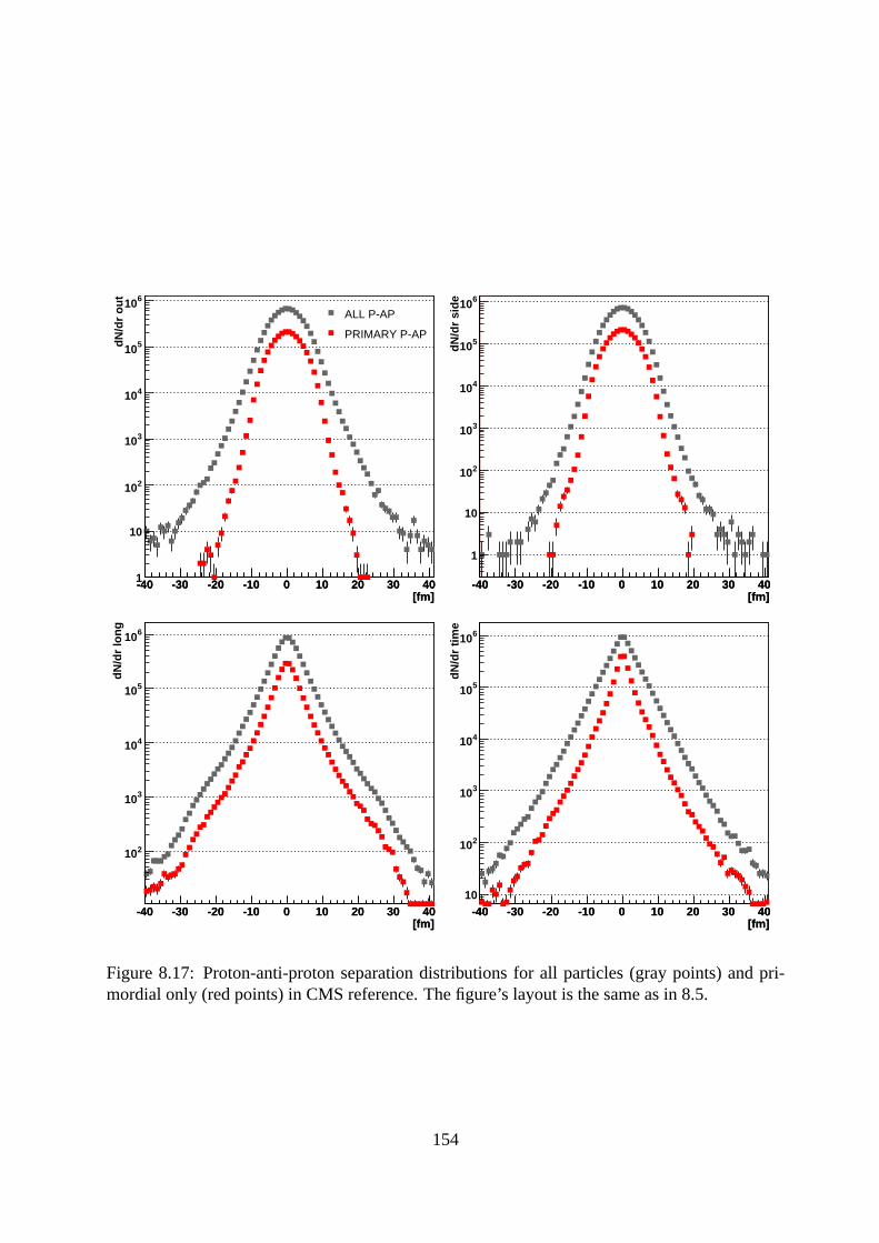
[fm]-40 -30 -20 -10 0 10 20 30 40

[fm]-40 -30 -20 -10 0 10 20 30 40

dN

/dr

ou

t

1

10

210

310

410

510

610ALL P-AP

PRIMARY P-AP

[fm]-40 -30 -20 -10 0 10 20 30 40

[fm]-40 -30 -20 -10 0 10 20 30 40

dN

/dr

sid

e

1

10

210

310

410

510

610

[fm]-40 -30 -20 -10 0 10 20 30 40

[fm]-40 -30 -20 -10 0 10 20 30 40

dN

/dr

lon

g

210

310

410

510

610

[fm]-40 -30 -20 -10 0 10 20 30 40

[fm]-40 -30 -20 -10 0 10 20 30 40

dN

/dr

tim

e

10

210

310

410

510

610

Figure 8.17: Proton-anti-proton separation distributions for all particles (gray points) and pri-mordial only (red points) in CMS reference. The figure’s layout is the same as in 8.5.

154

Figure 8.18: Pion-pion correlation function, left panel shows functions for QS and FSI included,right one illustrated correlations for QS only. Grey markershows correlation functions calculatedfor all particles, red marker indicates correlation functions for primordial particles only

(for positive values of separation). Each distribution does not represent a Gaussian shape (out

andside separations seen in the logarithmic scales- central parts represents Gaussian shape but

their tails imply non-Gaussian source distribution), whereas componentslong andtime do not

exhibit Gaussian form at all. The distributions forp−p andp−p systems are highly contaminated

by residual and nuclear remnants.

Correlations

Figure 8.18 shows identical pion correlations for QS calculations only (right panel) and QS+FSI

included (left panel), the second plot can be compared to theplot of correlation function calcu-

lated for the UrQMD model (Figure 8.8, left panel). This confirms what two-particle separation

distributions indicate: EPOS gives smaller source size than UrQMD, therefore the correlation

effect is stronger for the EPOS model.

The correlation function for pion-kaon combinations are shown in Figure 8.19; top panel of the

figure shows un-like signs combinations and the bottom panelshows like signs particle combi-

nations. Their ’double ratios’ are shown in Figure 8.20 (left panel for un-like signs and right

panel for like signs). Also in pion-kaon correlations for EPOS, the correlation effect is stronger

155

Figure 8.19: Pion-kaon (like signs in bottom panel and un-like signs at top panel) correlationfunction. Grey marker shows correlation functions calculated for all particles, red marker indi-cates correlation functions for primordial particles only

156

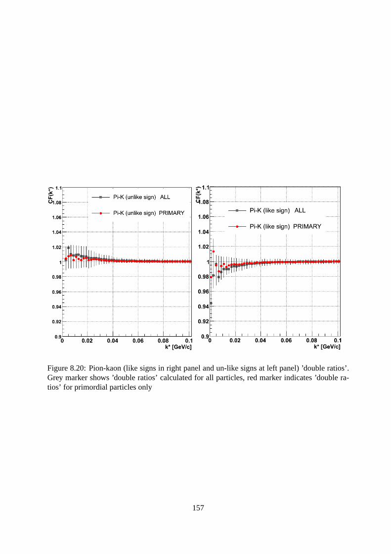
Figure 8.20: Pion-kaon (like signs in right panel and un-like signs at left panel) ’double ratios’.Grey marker shows ’double ratios’ calculated for all particles, red marker indicates ’double ra-tios’ for primordial particles only

157

than in UrQMD, which again indicates smaller source size (asbigger RMS values in two-particle

separation distributions). Another issue is the magnitudeof asymmetry: in EPOS it is weaker

than in UrQMD.

Figure 8.21 shows proton - anti-proton correlation functions. The correlation signal is clearly

visible. For pairs composed of primordial particles- the correlation effect is stronger. Top panel

presents correlation functions with respect to the sign ofk∗

out. The left-hand side of the bottom

part illustrates their ’double ratios’, which fluctuate around unity. As EPOS model does not con-

tain final particle rescattering implemented- the emissionof protons and anti-protons seems to

be similar to each other.

Asymmetry discussion

This section contains similar distributions as the sectiondedicated to the asymmetry discussion in

UrQMD. Figure 8.22 shows centrality dependence of proton - anti-proton separation distributions

in the CMS reference frame for primordial particles only. Allmean values forside and long

components are close to zero, however small deviation from zero is observed in distributions for

out direction andtime as well. For peripheral collisions the magnitude of asymmetry seems

to be the strongest and for central collisions the weakest. Even if they are reflected in both

separation distributions: forout andtime components, the deviations from zero are much smaller

and weaker than in the UrQMD model; they should not be interpreted as a clear evidence of

asymmetry in emission process between protons and anti-protons. Another two distributions can

be deduced for pion-kaon combinations from Tables 9.8 and 9.9 confirming what is observed in

the experiment and UrQMD model asymmetry in emission process between pions and kaons.

Table 9.7 collects results for two-pion system and confirms that in the case of identical particle

combinations no asymmetry is expected.

8.4.3 UrQMD and EPOS comparison

In terms of single-particle distributions (Figures 8.3, 8.13 and 8.4, 8.14), the EPOS model pre-

dicts observables similar to BRAHMS measurements. For separation distributions, both models

do not represent Gaussian shape of any source of particles. The comparison of mean values from

separation distribution is collected in Tables: 8.1 and 9.7-9.12.

Table 8.1 stores RMS and mean values for both models for three different centrality classes,

Tables 9.7, 9.8 and 9.9 contain these distribution characteristics for pion-pion, pion-kaon (like

158

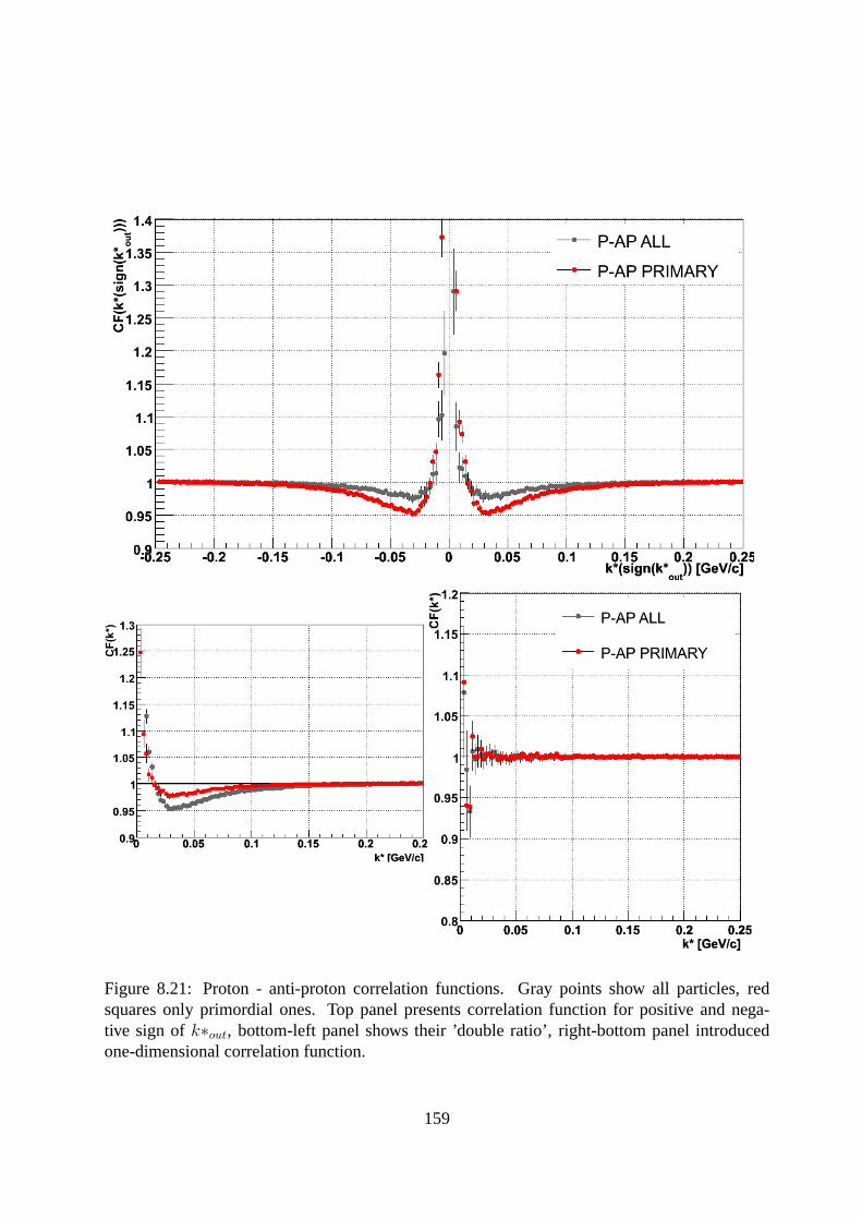
Figure 8.21: Proton - anti-proton correlation functions. Gray points show all particles, redsquares only primordial ones. Top panel presents correlation function for positive and nega-tive sign ofk∗out, bottom-left panel shows their ’double ratio’, right-bottom panel introducedone-dimensional correlation function.

159

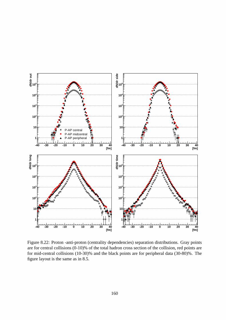
[fm]-40 -30 -20 -10 0 10 20 30 40

dN

/dr

ou

t

1

10

210

310

410

510

P-AP centralP-AP midcentralP-AP peripheral

[fm]-40 -30 -20 -10 0 10 20 30 40

dN

/dr

sid

e

1

10

210

310

410

510

[fm]-40 -30 -20 -10 0 10 20 30 40

dN

/dr

lon

g

1

10

210

310

410

510

[fm]-40 -30 -20 -10 0 10 20 30 40

dN

/dr

tim

e

1

10

210

310

410

510

Figure 8.22: Proton -anti-proton (centrality dependencies) separation distributions. Gray pointsare for central collisions (0-10)% of the total hadron crosssection of the collision, red points arefor mid-central collisions (10-30)% and the black points are for peripheral data (30-80)%. Thefigure layout is the same as in 8.5.

160

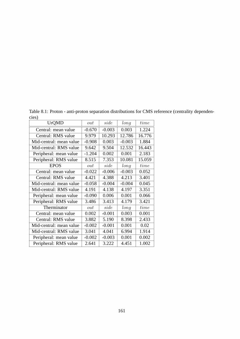
Table 8.1: Proton - anti-proton separation distributions for CMS reference (centrality dependen-cies)

UrQMD out side long time

Central: mean value -0.670 -0.003 0.003 1.224Central: RMS value 9.979 10.293 12.786 16.776

Mid-central: mean value -0.908 0.003 -0.003 1.884Mid-central: RMS value 9.642 9.504 12.532 16.443Peripheral: mean value -1.204 0.002 0.001 2.183Peripheral: RMS value 8.515 7.353 10.081 15.059

EPOS out side long timeCentral: mean value -0.022 -0.006 -0.003 0.052Central: RMS value 4.421 4.388 4.213 3.401

Mid-central: mean value -0.058 -0.004 -0.004 0.045Mid-central: RMS value 4.191 4.138 4.197 3.351Peripheral: mean value -0.090 0.006 0.001 0.066Peripheral: RMS value 3.486 3.413 4.179 3.421

Therminator out side long timeCentral: mean value 0.002 -0.001 0.003 0.001Central: RMS value 3.882 5.190 8.398 2.433

Mid-central: mean value -0.002 -0.001 0.001 0.02Mid-central: RMS value 3.041 4.041 6.994 1.914Peripheral: mean value -0.002 -0.003 0.001 0.002Peripheral: RMS value 2.641 3.222 4.451 1.002

161

signs) and pion-kaon (un-like signs) respectively. Another three tables: 9.10, 9.11 and 9.12

contain results proton - proton, anti-proton - anti-protonand proton - anti-proton systems re-

spectively. In all cases, RMS values are smaller for primordial particles only (smaller source

size) within the same model, the tendency of a bigger source for higher particle mass is observed

indicating that collective phenomena are applied in both models. EPOS reproduces stronger cor-

relations (smaller RMS values). Concerning correlation functions, source sizes follow tendencies

expressed in separation distributions. Both models can givereasonable correlation. Advanced

correlation techniques (as the method for non-identical particles) deduce relative shifts in time

and space between two particle’s species. In the case of proton - anti-proton correlation functions,

the correlation effect is stronger for UrQMD than for EPOS. Seen in data asymmetry in emission

process between protons and anti-protons is observed in UrQMD model as well. Hydrodynam-

ics does not reproduce any difference between protons and their anti-particles. Similar emission

properties of such particles are assumed. The generator Therminator which includes resonances

decays, but not rescattering processes, does not reflect such asymmetry as well (see Table 8.1).

EPOS model does not include hadron rescattering (only parton scatterings), thus no asymmetry

is seen. Finally UrQMD includes hadron rescatterings (hereobserved annihilation processes)

and space-time differences between protons and anti-protons emission are reproduced. STAR

data are not sensitive to the centrality dependence of space-time differences in emission process,

however UrQMD shows such tendency.

162

Chapter 9

Conclusions

The results of this work complement information obtained earlier by theHBT Physics Work-

ing groupof the STAR experiment at BNL. A detailed analysis performed already for identical

mesons: pions and kaons and the pioneer work with the pion-kaon correlations have reveal a

lot of unexpected effects commonly known asRHIC HBT puzzle. More information was clearly

necessary. This work is a step forward to fill this gap.

Considerably larger mass of baryons with respect to the mass of pions and kaons points out to a

new sort of information that can be obtained from the analysis of baryon correlations. Protons are

not so copiously produced as pions and their mean number at midrapidity is still larger than that

of antiprotons. The net-baryon free system has not been achieved yet at RHIC energies. The ther-

mal motion in the state of equilibrium, results in smaller mean velocity of protons with respect

to the velocity of lighter pions and kaons. On the other hand,the collective motion of particles

superimposed on the thermal one, gives a specific pattern of particle velocity distributions. As a

consequence, the final space time distribution of freeze-out points for different particle species

reflect the relations between thermal and collective motionof hot and expanding system created

in heavy ion collisions.

The length of homogeneity measured by femtoscopy methods includes the effects of space-

momentum correlations. Together with the relations between thermal and collective motions,

between chemical and thermal freeze-out, with the effects of resonance production and sec-

ondary rescattering the final image of space-time evolutionof the system represents a very com-

plex phenomena, difficult to quantitative description. A consistent description clearly needs the

information coming both from the analysis of light (pions) and heavy (protons) systems.

163

The following classes of two-particle systems, incident energies and event centralities have

been considered in the frame of this work:

• all combinations of two particle systems consisting of protons and antiprotons: (p − p),

(p − p,p − p),

• two energies of colliding gold nuclei: 200 GeV and 62 GeV per nucleon pair,

• three classes of event centralities, according to the percentage of the total hadronic cross-

section: central (0-10)%, mid-central (10-30)%, peripheral (30-80)%.

The following experimental results have been obtained:

• For the first time the analysis of two antiproton correlations has been performed and the

sizes of antiproton emission region in relativistic heavy ion collisions has been estimated.

• For the first time the analysis of two-particle correlationsfor all systems of protons and

antiprotons, simultaneously and in the same experimental conditions, has been performed.

The obtained quantitative results are consistent within the experimental uncertainties.

• For the first time the asymmetry between space-time parameters of proton and antiproton

emission has been analyzed and quantitatively estimated. Asmall asymmetry has been

found, showing that antiprotons are emitted earlier or moreclose to the edge of the emitting

system.

The analysis for all three proton/antiproton systems have been performed in the same way in all

energy/centrality classes; the same event selection criteria have been applied; the same correc-

tions have been introduced and the same approach was used to estimate the influence of residual

correlations. Thus the role of systematic errors was strongly reduced, what is important for the

quantitative comparison and for common analysis of all the results obtained in this work.

The following physics conclusions can be drawn:

• The measured values of proton/antiproton emission regionssizes are systematically smaller

then that of pions and kaons with similar transverse momenta. In frame of hydrodynamic

approach and taking into account the larger mass of protons with respect to kaons and

pions, one can understand it as an interplay of thermal and collective motion of hot and

expanding system. Thus, pairs of lighter particles are on average emitted from the region

of larger dispersion.

164

• The increase of measured sizes with the event centrality reflects the geometry of the col-

liding systems. This dependence is similar to that for pionsand kaons.

• The values of emission sizes obtained for 200GeV are slightly larger than those for 62GeV.

More statistics is necessary however to make quantitative conclusion.

• The obtained results are in qualitative agreement with the predictions of theoretical models:

UrQMD and EPOS. It is not the case however for the asymmetry results of nonidentical

particle correlations (see below).

• A small, but definitively nonzero, asymmetry shift have beenfound in the analysis of

proton-antiproton correlations. One should mention here that a relatively large shift was

experimentally found earlier for the pion-kaon system. This result is consistent with the

hydrodynamic description, where the mass differences leadto the space-time asymmetries.

Such effect cannot be attributed however to the particles with the same masses. The asym-

metry shift is also absent in the results of simulations withthe EPOS model but is seen in

the results of UrQMD simulations. As the difference betweenEPOS and UrQMD, impor-

tant for the final stage of the interaction dynamics, is the absence of rescattering processes

in the EPOS model, one can conclude that the annihilation processes at the last stage of

the collision can be responsible for the observed asymmetry. This conclusion is also con-

sistent with the sign of asymmetry effect, showing that antiprotons are emitted earlier or

more close to the edge of the emitting system than protons.

In order to obtain the physics results free of experimental distortions some specific kinds of

methodical analysis have been performed.

• A set of cuts have been applied for the registered tracks to eliminate the merging effect

which makes that instead of two separate tracks, only one is reconstructed.

• A dedicated analysis of the tracks located very close in the detector space have been per-

formed in order to avoid the splitting effect which causes that instead of one single track,

two track are found.

• The contamination of electron - positron pairs have been removed.

• The effect of finite detector resolution have been taken intoaccount as well.

165

• A special attention have been put to the effect of residual correlations resulting mainly

from the contamination of the proton/antiproton sample by the particles (also protons or

antiprotons) coming from the week decays of hyperons. This effect is much more dan-

gerous for protons than for pions. The kinematics of lambda-hyperon decay makes that

proton practically follow the direction of lambda particlein the detector space and can-

not be distinguished experimentally from that coming directly from the interaction point.

A detailed procedure have been developed and the decays of lambda and sigma hyperons

have been considered, including the decay kinematics. The reflection of FSI correlations in

the proton/antiproton hyperon systems, in the studied proton-antiproton correlations have

been taken into account. One should mention here that such analysis was made for the first

time in the analysis of correlations for the baryonic systems. This can be important for the

comparison of the results obtained here with the other results obtained elsewhere, where

the residual correlations have not been taken into account properly.

The analysis performed here is a step forward in the direction of consistent description of the

dynamics of heavy ion collisions, mainly in the part of so called soft processes.

The next steps can be the following:

• Complete the existing results for meson-meson and baryon-baryon systems by the analysis

of meson-baryon correlations. It can serve as an important consistency test.

• Perform the analysis with larger statistics for more centrality bins.

• Continue the asymmetry analysis, also with larger statistics.

• Make the analysis and find the source sizes in three dimensions: out, side andlong. It will

allow one to obtain information about the shape of the source.

• Perform common analysis of source sizes for different particle systems and for different

transverse mass intervals. It will allow one to measure estimate the effects of collective

motions with higher precision.

• Make the azimuthally-sensitive two-proton correlation studies. It will help to assess the

source-size depending on reaction plane and to find the relations between the geometry

and dynamic factors in heavy ion collisions

In order to perform the analysis proposed above it is necessary to have more statistics of experi-

mental data. In a natural way it can be achieved in the next generation experiment ALICE being

166

prepared now at CERN. Much larger particle multiplicities andthe better detection possibilities

makes good perspectives for such measurements. However, atthe LHC conditions it is not clear

what one would expect. As nobody knows what system will be created (QGP or sQGP), it is not

possible to predict what results concerning femtoscopy should be expected. On the other hand, it

seems to be reasonable to check what RHIC II will bring as the accelerator and detector upgrades

will allow to analyze data in the collision energy closer to the present RHIC observable. RHIC

II plans to collect data with much higher luminosity that RHICcould do, so the following field

of research are the main topic of interest:

• High PT

• Heavy Flavor

• Equation of State

• Electromagnetic Probes

• Forward Physics

• Spin

The correlation analysis might be very interesting, however the program to study such measure-

ments is not worked out.

167

Appendix 1- Elementary units, particles

and their interactions

Elementary units

The basic units in physics are length, mass and time and the SIsystem expresses them in meters,

kilograms and seconds. These units are not very appropriatein high energy physics, where

typical lengths are10−15m and typical masses are10−27kg. The above table introduces basic

units used in high energy physics. In calculations, the quantities of Planck constant and speed of

light occur frequently, so their units are set to:~ = h2π

= c = 1. Basic units are listed below.

Quantity High energy units Value of SI units

length 1 fm 10−15m

energy 1 GeV=109 eV 1.602× 10−10 J

mass 1 GeV/c2 1.78× 10−27 kg

~ = h/(2π) 6.588× 10−25 GeV s 1.055× 10−34 J s

c 2.998× 1023 fm/s 2.998× 108 m/s

~c 0.1975 GeV fm 3.162× 10−26 J m

Particle classification

Fundamental particles [98] are of two types: particles withhalf-integer spin are called fermions

because they obey Fermi-Dirac Statistic, while those with integer spin obey Bose-Einstein statis-

tics and are called bosons. The statistics obeyed by a particles determine how the wave function

Ψ describing an assemble of identical particles behaves under interchange of any pair of parti-

cles, say 1 and 2. The theory says that under exchange of identical bosonsΨ is symmetric and

under exchange of identical fermionsΨ is anti-symmetric.

168

Fundamental fermions

The experimental data from high-energy experiments can be described by Standard Model [12,

13] of particles and their interactions, formulated in the second part of twentieth century. Ac-

cording to this model, all mater is built up from a small number of fundamental spin1/2 particles

(fermions): 6 quarks and 6 leptons. For each constituent, its symbol and a ratio of of its electric

chargeQ to elementary chargee are given in the Table 9.1.

Table 9.1: A list of elementary fermions.Particle Flavor Q/|e|

leptons e µ τ -1νe νµ ντ 0

quarks u c t +2/3d s b -1/3

• Leptons

The leptons carry integer electric charge, the electrone is familiar to everybody and other leptons

are muonµ and taonτ , heavier than electron. The neutral leptons are called “neutrinos” ν. A

different flavor of neutrinos (e, µ, τ ) is paired with each flavor of charged leptons. Neutrinos were

postulated by Pauli in 1930 in order to explain energy and momentum missing in the process of

nuclearβ decay, where an electron is emitted together with its neutrinoνe. The masses and mass

limits are collected in Table 9.2.

Table 9.2: The masses of leptons taken from Particle PhysicsBooklet, edition 2004.Flavor Charge lepton massNeutron lepton mass

e me=0.511 MeV mνe< 3eV

µ mµ=105.658 MeV mνµ< 0.19 MeV

τ mτ=1776.990 MeV mντ< 18.2 MeV

• Quarks

Quarks [99] (see Table 9.3) carry fractional charges of+23|e| or −1

3|e|. Two quarks:b andt are

called as ’beauty’ or ’true’ respectively as well. Leptons exist as free particles but quarks do

169

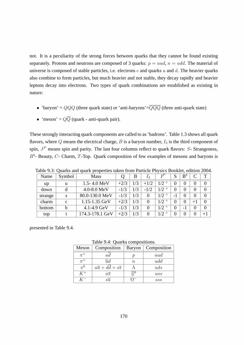
not. It is a peculiarity of the strong forces between quarks that they cannot be found existing

separately. Protons and neutrons are composed of 3 quarks:p = uud, n = udd. The material of

universe is composed of stable particles, i.e. electronse and quarksu andd. The heavier quarks

also combine to form particles, but much heavier and not stable, they decay rapidly and heavier

leptons decay into electrons. Two types of quark combinations are established as existing in

nature:

• ’baryon’ = QQQ (three quark state) or ’anti-baryons’=QQQ (three anti-quark state)

• ’meson’ =QQ (quark - anti-quark pair).

These strongly interacting quark components are called to as ’hadrons’. Table 1.3 shows all quark

flavors, whereQ means the electrical charge,B is a baryon number,I3 is the third component of

spin,JP means spin and parity. The last four columns reflect to quark flavors:S- Strangeness,

Bb- Beauty,C- Charm,T -Top. Quark composition of few examples of mesons and baryons is

Table 9.3: Quarks and quark properties taken from Particle Physics Booklet, edition 2004.Name Symbol Mass Q B I3 JP S Bb C T

up u 1.5- 4.0 MeV +2/3 1/3 +1/2 1/2 + 0 0 0 0down d 4.0-8.0 MeV -1/3 1/3 -1/2 1/2 + 0 0 0 0

strange s 80.0-130.0 MeV -1/3 1/3 0 1/2 + -1 0 0 0charm c 1.15-1.35 GeV +2/3 1/3 0 1/2 + 0 0 +1 0bottom b 4.1-4.9 GeV -1/3 1/3 0 1/2 + 0 -1 0 0

top t 174.3-178.1 GeV +2/3 1/3 0 1/2 + 0 0 0 +1

presented in Table 9.4.

Table 9.4: Quarks compositions.Meson Composition Baryon Composition

π+ ud p uudπ+ ud n udd

π0 uu + dd + ss Λ udsK+ us Ξ0 ussK− su Ω− sss

170

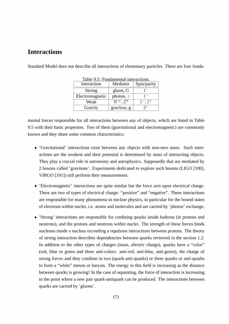
Interactions

Standard Model does not describe all interactions of elementary particles. There are four funda-

Table 9.5: Fundamental interactions.Interaction Mediator Spin/parity

Strong gluon, G 1−

Electromagnetic photon,γ 1−

Weak W±, Z0 1−, 1+

Gravity graviton, g 2+

mental forces responsible for all interactions between anyof objects, which are listed in Table

9.5 with their basic properties. Two of them (gravitationaland electromagnetic) are commonly

known and they share some common characteristics.

• ’Gravitational’ interactions exist between any objects with non-zero mass. Such inter-

actions are the weakest and their potential is determined bymass of interacting objects.

They play a crucial role in astronomy and astrophysics. Supposedly that are mediated by

2 bosons called ’gravitons’. Experiments dedicated to explore such bosons (LIGO [100],

VIRGO [101]) still perform their measurements.

• ’Electromagnetic’ interactions are quite similar but the force acts upon electrical charge.

There are two of types of electrical charge: “positive” and “negative”. These interactions

are responsible for many phenomena in nuclear physics, in particular for the bound states

of electrons within nuclei, i.e. atoms and molecules and arecarried by ’photon’ exchange.

• ’Strong’ interactions are responsible for confining quarksinside hadrons (in protons and

neutrons), and the protons and neutrons within nuclei. The strength of these forces binds

nucleons inside a nucleus exceeding a repulsion interactions between protons. The theory

of strong interaction describes dependencies between quarks reviewed in the section 1.2.

In addition to the other types of charges (mass, electric charge), quarks have a “color”

(red, blue or green and three anti-colors: anti-red, anti-blue, anti-green), the charge of

strong forces and they combine in two (quark-anti-quarks) or three quarks or anti-quarks

to form a “white” meson or baryon. The energy in this field is increasing as the distance

between quarks is growing! In the case of separating, the force of interaction is increasing

to the point where a new pair quark-antiquark can be produced. The interactions between

quarks are carried by ’gluons’.

171

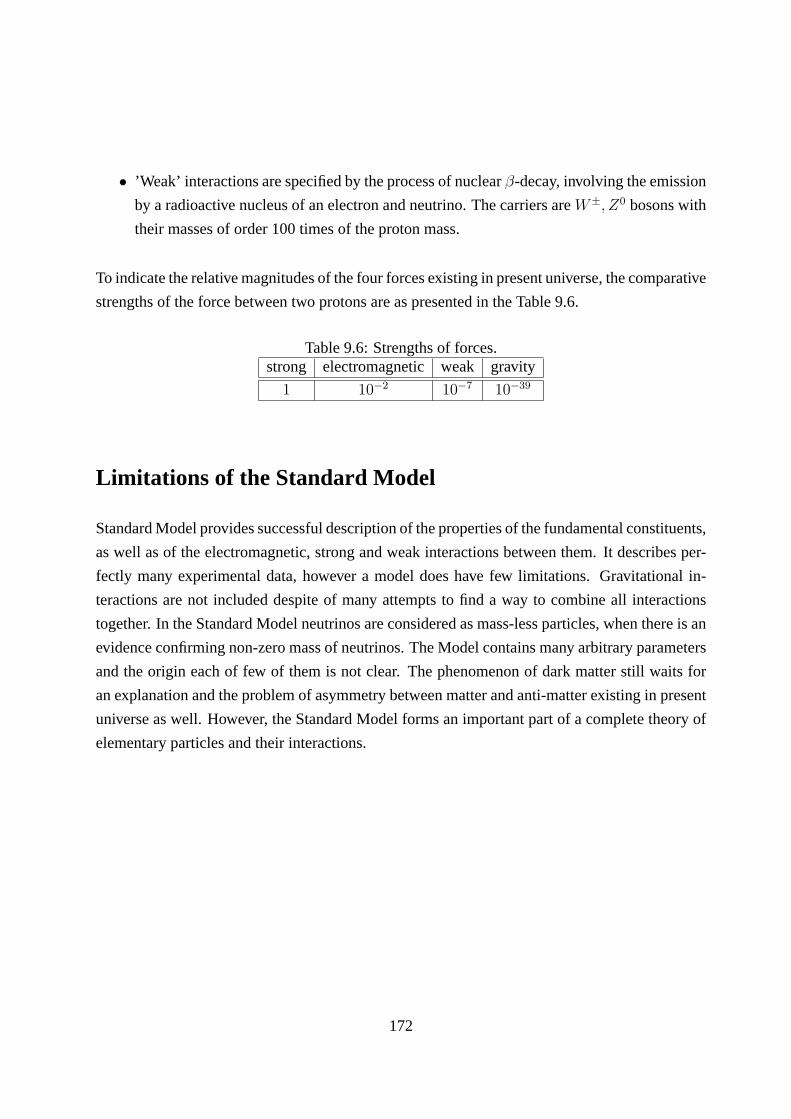
• ’Weak’ interactions are specified by the process of nuclearβ-decay, involving the emission

by a radioactive nucleus of an electron and neutrino. The carriers areW±, Z0 bosons with

their masses of order 100 times of the proton mass.

To indicate the relative magnitudes of the four forces existing in present universe, the comparative

strengths of the force between two protons are as presented in the Table 9.6.

Table 9.6: Strengths of forces.strong electromagnetic weak gravity

1 10−2 10−7 10−39

Limitations of the Standard Model

Standard Model provides successful description of the properties of the fundamental constituents,

as well as of the electromagnetic, strong and weak interactions between them. It describes per-

fectly many experimental data, however a model does have fewlimitations. Gravitational in-

teractions are not included despite of many attempts to find away to combine all interactions

together. In the Standard Model neutrinos are considered asmass-less particles, when there is an

evidence confirming non-zero mass of neutrinos. The Model contains many arbitrary parameters

and the origin each of few of them is not clear. The phenomenonof dark matter still waits for

an explanation and the problem of asymmetry between matter and anti-matter existing in present

universe as well. However, the Standard Model forms an important part of a complete theory of

elementary particles and their interactions.

172

Appendix 2- Symbols and conventions used

This part define the formulas which are used for two-particleseparation distributions. In terms

of two-particle correlations, distinguishable particles1 and2 are considered. Each particle is

described by its coordinates of freeze-out: spatialx, y, z and time:t (four-vectorx = t,−→x ),

and by its momentum coordinates:px, py, pz (momentum) andE (energy) (four-momentum

p = E,−→p ) in the reference frame of the emitting source (CMS). When two particles are

combined into a pair, a new reference frame can be introduced, a frame where the center-of-mass

of the pair rests. This frame is called Pair Rest Frame (PRF). Values in PRF are marked with

asterrisks *.

The total momentum of pair

P = p1 + p2 = 2p (9.1)

and the relative momentum of pair

q = p1 − p2 (9.2)

are the most important quantities. For non-identical particles are generalized momentum differ-

ence is defined:

q = q − P(qP)/P2 (9.3)

In PRF the one has

q = 0, 2−→k∗ (9.4)

wherek∗ is the momentum of first particle of pair in PRF. In CMS one also has the spatial

coordinate

X = [(P1P)x1 + (p2P)x2]/P2 (9.5)

Also new directions can be defined, similar to theout, side andlong decompositions of Bertsch

and Pratt. Thelong direction is the direction of beam axis, orz. In the transverse plane theout

(or x) direction is the one of the momentum of the pair−→P , andside (or y) is perpendicular to

out andlong.

173

Pair separation can also be calculated:

−→r = −→r1 −−→r2 (9.6)

Thetime difference:

∆t = t1 − t2 (9.7)

Both of the variables can be calculated in the PRF and then they are denoted as−→r∗ andt∗.

For non-identical particles it is significant which particle is first and which is second, as the signs

of −→r and−→q depend on ordering. Therefore a convention is adopted that the first particle is

always the one with lower mass, if both particles have the same masses, the one with larger value

of charge is taken as first.

The procedure of decomposition of−→r∗ and

−→k∗ into out, side andlong is described below. First,

the pair is boosted to the Longitudinally Co-Moving System (LCMS), that is the system where:

p1,z = −p2,z (9.8)

along thez axis with velocity

βz = |pz|/E (9.9)

Then

k∗

long = pLCMS1,z = −pLCMS

2,z (9.10)

r∗long = r1,z − r2,z (9.11)

Then a pair is rotated so that itsx axis is along the pair transverse momentum. Then a pair is

boosted to the PRF alongx axis with

βt = |pt|/(E2 − p2z) (9.12)

Other components are given:

k∗

out = pPRF1,x = −pPRF

2,x (9.13)

and

k∗

side = pPRF1,y = −pPRF

2,y (9.14)

Similarly:

r∗out = rPRF1,x − rPRF

2,x (9.15)

174

and

r∗side = rPRF1,y − rPRF

2,y (9.16)

The initial separation in CMS−→r can also be decomposed into three components:rout, rside,

rlong. Simple relations between the pair separation in two reference frames are given:

r∗side = rside (9.17)

r∗long = γz(rlong − βz∆t) (9.18)

∆tLCMS = γz(∆t − βzrlong) (9.19)

r∗out = γt(rout − βt∆tLCMS) (9.20)

t∗ = γt(∆tLCMS − βtrout) (9.21)

whereγz = (1 − β2z )

−1/2 andγt = (1 − β2t )

−1/2.

175

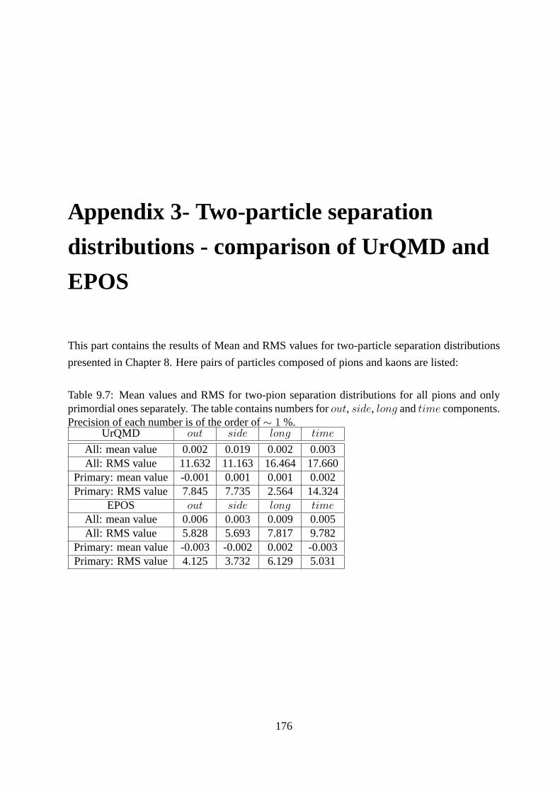
Appendix 3- Two-particle separation

distributions - comparison of UrQMD and

EPOS

This part contains the results of Mean and RMS values for two-particle separation distributions

presented in Chapter 8. Here pairs of particles composed of pions and kaons are listed:

Table 9.7: Mean values and RMS for two-pion separation distributions for all pions and onlyprimordial ones separately. The table contains numbers forout, side, long andtime components.Precision of each number is of the order of∼ 1 %.


All: mean value 0.002 0.019 0.002 0.003All: RMS value 11.632 11.163 16.464 17.660

Primary: mean value -0.001 0.001 0.001 0.002Primary: RMS value 7.845 7.735 2.564 14.324

EPOS out side long timeAll: mean value 0.006 0.003 0.009 0.005All: RMS value 5.828 5.693 7.817 9.782

Primary: mean value -0.003 -0.002 0.002 -0.003Primary: RMS value 4.125 3.732 6.129 5.031

176

Table 9.8: Mean values and RMS for pion-kaon (like signs) separation distributions for all par-ticles and only primordial ones separately. The table contains numbers forout, side, long andtime components. Precision of each number is of the order of∼ 1 %.


All: mean value -2.102 0.002 0.003 0.910All: RMS value 11.316 10.261 15.707 17.474


EPOS out side long timeAll: mean value -0.623 0.000 0.012 0.523All: RMS value 5.827 5.060 7.350 7.443


Table 9.9: Mean values and RMS for pion-kaon (un-like signs) separation distributions for allparticles and only primordial ones separately. The table contains numbers forout, side, longandtime components. Precision of each number is of the order of∼ 1 %.




EPOS out side long timeAll: mean value -0.626 0.000 0.005 0.277All: RMS value 5.820 5.059 7.338 7.427


177

Table 9.10: Mean values and RMS for two-proton separation distributions for all particles andonly primordial ones separately. The table contains numbers for out, side, long andtime com-ponents. Precision of each number is of the order of∼ 1 %.



Primary: mean value 0.001 0.002 0.001 0.001Primary: RMS value 9.517 8.397 11.366 16.527

EPOS out side long timeAll: mean value -0.004 0.002 0.006 -0.004All: RMS value 4.344 3.955 4.611 4.516

Primary: mean value 0.003 0.000 0.000 -0.003Primary: RMS value 3.763 3.714 4.268 3.435

Table 9.11: Mean values and RMS for two - anti-proton separation distributions for all particlesand only primordial ones separately. The table contains numbers forout, side, long andtimecomponents. Precision of each number is of the order of∼ 1 %.




EPOS out side long timeAll: mean value -0.013 0.005 -0.009 -0.003All: RMS value 4.372 3.966 4.541 4.507

Primary: mean value -0.008 -0.002 -0.001 -0.001Primary: RMS value 3.798 3.712 4.138 3.403

178

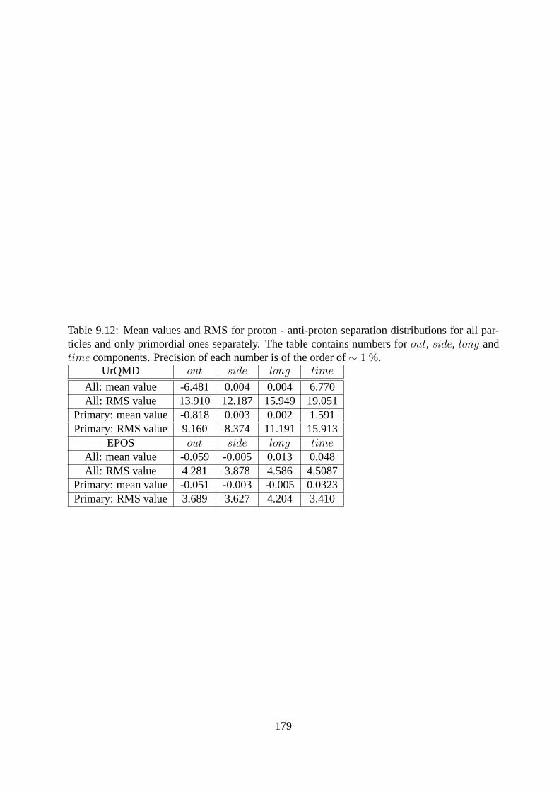
Table 9.12: Mean values and RMS for proton - anti-proton separation distributions for all par-ticles and only primordial ones separately. The table contains numbers forout, side, long andtime components. Precision of each number is of the order of∼ 1 %.




EPOS out side long timeAll: mean value -0.059 -0.005 0.013 0.048All: RMS value 4.281 3.878 4.586 4.5087

Primary: mean value -0.051 -0.003 -0.005 0.0323Primary: RMS value 3.689 3.627 4.204 3.410

179

Glossary

Presented definitions refer to the subject of discussed herework. They may not contain full

information about defined term.

Anti-particle - a particle associated with every particle, it is characterized by exactly the same

mass and life-time, but opposite values of electric charge,magnetic moment, baryon num-

ber and flavor.

Baryon - the family of subatomic particles which are made of three quarks. The family includes

the proton and neutron, which build up the atomic nucleus.

Big Bang - the cosmological model of the universe whose primary assertion is that the universe

has expanded into its current state from a primordial condition of enormous density and

temperature.

Boson - particles with an integer spin, they obey Bose-Einstein statistics, i.e. the wave-function

describing two identical bosons is symmetric under particle exchange.

Bottom quark - quark which is also called ’beauty’ quark, it has electric charge−1/3|e|, it was

discovered in the form of upsilon meson (bb).

Charm quark, charmonium - quark of electric charge+2/3|e|, it forms charmonium state

J/Ψ = cc

Chirality - Mathematically, it is the sign of the projection of the spinvector onto the momentum.

Mass-less particles such as the photon or the gluon have absolute chirality: a mass-less

particle appears to have spin in the same direction along itsaxis of motion regardless of

point of view of the observer. A mass-less particle moves with the speed of light, so a

real observer (who must always moves slower than the speed oflight) cannot be in any

reference frame where the particle appears to reverse its relative direction, meaning that

180

all real observers see the same chirality. Because of this, the direction of spin of mass-less

particles is not affected by a Lorentz boost (change of viewpoint) in the direction of motion

of the particle, and chirality is fixed for all reference frames, it is absolute. Particles which

do have mass such as electrons or quarks have relative chirality, which depends on the

observer’s reference frame. In the case of these particles,it is possible for an observer to

change to a reference frame that overtakes the spinning particle, in which case the particle

will then appear to move backwards, and its apparent chirality will reverse.item [Color] -

a fundamental property of quarks, was given to the strong charge of quarks, which interact

with each other. As more than one fermion cannot exist in the same state with another

fermion, color differs them.

Collider - a type of a particle accelerator involving two beams of particles approaching directly

against each other. Particles collide moving in opposite directions.

Confinement - a property of strong color interaction between quarks, where quarks cannot exist

in a single states, but they has to be bound inside hadrons.

Correlation function (of two particles with close velocities) - a function illustrating FSI and/or

QS (depending on system) which allows one to deduce source size.

Cross section- the rate of particular reaction. This is an effective area subtended by the target

particle to an incident beam. It is numerically equal to the reaction rate per target particle

per unit incident flux.

Debye-screening- The effect known in electrostatics, in the case of few electric charges, the

effective potential of interaction depends on e.g. Debye screening radius, which lead to that

the electrical charge of some sources is screened by anotherones. Then, it was proposed

that similar screening can occur in QGP, and the interactionbetween quark ’c’ and their

anti-quark (J/Psi particle) becomes weaker with increasing their relative distance; thus

production ofJ/Psi particle was proposed as one of signature of QCD.

Fermion - particles with a half-integer spin, such as protons and electrons. They obey Fermi-

Dirac statistics, i.e. the wave-function describing two identical fermions is anti-symmetric

under particle exchange.

Flavor - a generic name to describe different types of quarks (up, down, strange, charm, top,

bottom).

181

FSI - Final State Interaction (Coulomb and Strong) present during final state of source evolution,

in two-particle correlations FSI are reflected in the shape of correlation function

Flow - a collective motion of matter created in heavy-ion collisions.

Freeze-out - final part of hadronization, it can be thermal or chemical. After this part of source

evolution- hadrons and other products move to detector and can be identified in the case,

when do not decay before registration.

Gluon - elementary particle that cause quarks to interact, and is indirectly responsible for the

binding of protons and neutrons together in atomic nuclei.

Hadron - strongly interacting composite subatomic particle. All hadrons are composed of

quarks. Hadrons are divided into classes of mesons and baryons.

Hadronization - the process of the formation of hadrons out of quarks and gluons.

Hyperon - subatomic particle which is a baryon (and hence a hadron anda fermion) with non-

zero strangeness, but with zero charm and zero bottomness.

Hydrodynamics - is a branch of theoretical fluid dynamics which deals with flow of an ideal

fluid. An ideal fluid is both incompressible and inviscid.

Impact parameter b - parameter describing a collision centrality; it is the length of vector con-

necting centers of collided nuclei, while nuclei are collided. In the case of central col-

lisions, parameter [b]=0, for non-central ones can achieveeven two radii of nuclei; for

ultra-peripheral collisions it exceeds [2R] (in symmetric collisions of two identical nuclei,

where [R] is the radius of one nucleus).

Isospin - a quantum number related to the strong interaction and applies to the interactions of

the neutron and proton, it differs proton and neutron.

Jet - a stream of particles produced in hard processes.

Meson - a strongly interacting boson, a hadron with integral spin,it is composed of combination

of valence quark and anti-quark.

Mini-jet - is a pair of partons which go in opposite directions (like standard jet), but their trans-

verse momentum can be considered as a lower limit of hard processes (pt ≥ 2 GeV).

Participant (of a collision) - part of collided nuclei which directly take part in the collision.

182

Resonance- unstable hadron due to strong interactions.

SH - Spherical Harmonics are angular portion of an orthogonal set of solutions to Laplace’s

equation represented in a system of spherical coordinates.

Spectator (of a collision) - nucleon from collided nuclei that does nottake part during collision

directly.

QED - Quantum electrodynamics (is a relativistic quantum field theory of electrodynamics.

QED was developed by a number of physicists, beginning in thelate 1920s, it mathe-

matically describes all phenomena involving electricallycharged particles interacting by

means of exchange of photons.

QCD - Quantum chromodynamics is theory of the strong interaction (color force), a fundamen-

tal force describing the interactions of the quarks and gluons found in hadrons (such as the

proton, neutron or pion). QCD is a quantum field theory of a special kind called a non-

abelian gauge theory. It is an important part of the StandardModel of particle physics. A

huge body of experimental evidence for QCD has been gathered over the years.

QGP - a quark-gluon plasma is a phase of quantum chromodynamics (QCD) which exists at

extremely high temperature and/or density. This phase consists of (almost) free quarks and

gluons which are the basic building blocks of matter.

QS - Quantum Statistics, a calculation of quantum mechanics for identical fermions or bosons.

Rapidity - a variable connects energy and longitudinal component of momentum:y = 12ln

(

E+pz

E−pz

)

.

Another relations are given:dy = dpZ

E, cosy= E

mTandsiny= pz

mT, wheremT =

√

m2 + p2T

is a transverse mass andE =√

p2 + m2.

Thermodynamics - a branch of physics that studies the effects of changes in temperature, pres-

sure, and volume on physical systems at the macroscopic scale by analyzing the collective

motion of their particles using statistics.

183

List of publications

1. Forward Lambda production and nuclear stopping power in d+ Au collisions at√

sNN =

200 GeV; STAR Collaboration (B.I. Abelev, H.P. Gos et al.); Submitted to Phys.Rev.C;

arXiv:0706.0472 [nucl-ex]

2. Measurement of transverse single-spin asymmetries for di-jet production in proton-proton

collisions at√

sNN = 200GeV; STAR Collaboration (B.I. Abelev, H.P. Gos et al.);

Phys.Rev.Lett.99:142003,2007; arXiv:0705.4629 [hep-ex]

3. Proton proton, anti-proton anti-proton, proton anti-proton correlations in Au + Au colli-

sions measured by STAR at RHIC; H.P. Gos; Eur.Phys.J.C49:75-80,2007.

4. Enhanced strange baryon production in Au + Au collisions compared to p + p at√

sNN =

200GeV; STAR Collaboration (B.I. Abelev, H.P. Gos et al.); Submitted to Phys.Rev.Lett,

arXiv:0705.2511 [nucl-ex]

5. Global polarization measurement in Au+Au collisions; STAR Collaboration (B.I. Abelev,

H.P. Gos et al.); Phys.Rev.C76:024915,2007; arXiv:0705.1691 [nucl-ex]

6. Energy dependence of pi+-, p and anti-p transverse momentum spectra for Au+Au col-

lisions at√

sNN = 62 and200GeV; STAR Collaboration (B.I. Abelev, H.P. Gos et al.);

Phys.Lett.B655:104-113,2007; nucl-ex/0703040

7. Partonic flow and phi-meson production in Au + Au collisions at√

sNN = 200GeV;

STAR Collaboration (B.I. Abelev, H.P. Gos et al.); Phys.Rev.Lett.99:112301,2007; nucl-

ex/0703033

8. Charged particle distributions and nuclear modification at high rapidities in d + Au colli-

sions at√

sNN = 200GeV; STAR Collaboration (B.I. Abelev, H.P. Gos et al.); Submitted

to Phys.Lett.B; nucl-ex/0703016

184

9. Mass, quark-number, and√

sNN dependence of the second and fourth flow harmonics in

ultra-relativistic nucleus-nucleus collisions; STAR Collaboration (B.I. Abelev, H.P. Gos et

al.); Phys.Rev.C75:054906,2007; nucl-ex/0701010

10. Baryon - baryon correlations in Au+Au collisions at√

sNN = 62 and√

sNN = 200GeV,

measured in the STAR experiment at RHIC; H.P. Gos; Nukleonika,Vol. 51, supplement 3,

nucl-ex/0610030

11. Rapidity and species dependence of particle production at large transverse momentum for

d+Au collisions at√


Phys.Rev.C76:054903,2007; nucl-ex/0609021

12. Longitudinal double-spin asymmetry and cross section for inclusive jet production in po-

larized proton collisions at√

sNN = 200GeV; STAR Collaboration (B.I. Abelev, H.P. Gos

et al.); Phys.Rev.Lett.97:252001,2006; hep-ex/0608030

13. Neutral kaon interferometry in Au+Au collisions at√

sNN = 200GeV; STAR Collabora-

tion (B.I. Abelev, H.P.Gos et al.); Phys.Rev.C74:054902,2006; nucl-ex/0608012

14. Strange particle production in p+p collisions at√

sNN = 200GeV; STAR Collaboration

(B.I. Abelev, H.P. Gos et al.); Phys.Rev.C75:064901,2007; nucl-ex/0607033

15. Transverse momentum and centrality dependence of high-p(T) non-photonic electron sup-

pression in Au+Au collisions at√

sNN = 200GeV; STAR Collaboration (B.I. Abelev, H.P.

Gos et al.); Phys.Rev.Lett.98:192301,2007; nucl-ex/0607012

16. Delta phi Delta eta Correlations in Central Au+Au Collisions at√

sNN = 200GeV; STAR

Collaboration (J. Adams, H.P. Gos et al.); Phys.Rev.C75:034901,2007; nucl-ex/0607003

17. The particle interferometry method as a tool reflecting evolution of hadron source; H.P.

Gos; AIP Conf.Proc.828:458-463,2006

18. The Multiplicity dependence of inclusive p(t) spectra from p-p collisions at√

sNN =

200GeV; STAR Collaboration (J. Adams, H.P. Gos et al.); Phys.Rev.D74:032006,2006;

nucl-ex/0606028

19. Scaling Properties of Hyperon Production in Au+Au Collisions at√

sNN = 200GeV;

STAR Collaboration (J. Adams, H.P. Gos et al.); Phys.Rev.Lett.98:062301,2007; nucl-

ex/0606014

185

20. Identified baryon and meson distributions at large transverse momenta from Au+Au colli-

sions at√


Phys.Rev.Lett.97:152301,2006; nucl-ex/0606003

21. The Energy dependence of p(t) angular correlations inferred from mean-p(t) fluctuation

scale dependence in heavy ion collisions at the SPS and RHIC; STAR Collaboration (J.

Adams, H.P. Gos et al.); J.Phys.G33:451-466,2007; nucl-ex/0605021

22. Strange baryon resonance production in√

sNN = 200GeV p+p and Au+Au collisions;

STAR Collaboration (J. Adams, H.P. Gos et al.); Phys.Rev.Lett.97:132301,2006; nucl-

ex/0604019

23. Direct observation of di-jets in central Au+Au collisions at√

sNN = 200GeV;STAR Col-

laboration (J. Adams, H.P. Gos et al.); Phys.Rev.Lett.97:162301,2006; nucl-ex/0604018

24. Forward neutral pion production in p+p and d+Au collisions at√

sNN = 200GeV; STAR

Collaboration (J. Adams, H.P. Gos et al.); Phys.Rev.Lett.97:152302,2006; nucl-ex/0602011

25. Measurements of identified particles at intermediate transverse momentum in the STAR

experiment from Au + Au collisions at√

sNN = 200GeV; STAR Collaboration (J. Adams,

H.P. Gos et al.); Submitted to Phys.Rev.C; nucl-ex/0601042

26. Identified hadron spectra at large transverse momentum in p+p and d+Au collisions at√

sNN = 200GeV; STAR Collaboration (J. Adams, H.P. Gos et al.); Phys.Lett.B637:161-

169,2006; nucl-ex/0601033

27. Recent high-PT Results from STAR; STAR Collaboration (C.A. Gagliardi, H.P. Gos et al.);

Eur.Phys.J.C43:263-270,2005

28. Charm Production in the STAR Experiment at RHIC, By STAR Collaboration (A.A.P.

Suaide, H.P. Gos et al.). 2005, Eur.Phys.J.C43:193-200,2005

29. Open Charm Production from d+Au Collisions in STAR, STAR Collaboration (M. Calderon

de la Barca Sanchez, H.P. Gos et al.); Eur.Phys.J.C43:187-192,2005

30. Strangelet Search at RHIC, STAR Collaboration (J. Adams, H.P. Gos et al.); Phys.Rev.C76:

011901,2007; nucl-ex/0511047

186

31. Multiplicity and Pseudorapidity Distributions of Charged Particles and Photons at Forward

Pseudorapidity in Au+Au Collisions at√

sNN = 62GeV; STAR Collaboration (J. Adams,

H.P. Gos et al.); Phys.Rev.C73:034906,2006; nucl-ex/0511026

32. Proton - lambda correlations in central Au+Au collisions at√

sNN = 200GeV; STAR

Collaboration (J. Adams, H.P. Gos et al.); Phys.Rev.C74:064906,2006; nucl-ex/0511003

33. Directed Flow in Au+Au Collisions at√

sNN = 62GeV, STAR Collaboration (J. Adams,


34. Transverse Momentum p(T) Correlations on (Eta, Phi) fromMean p(T) Fluctuations in

Au+Au Collisions at√

sNN = 200 GeV, STAR Collaboration (J. Adams, H.P. Gos et al.);

J.Phys.G32:L37-L48,2006; nucl-ex/0509030

35. Incident Energy Dependence of p(T) Correlations at RHIC; STAR Collaboration (J. Adams,


36. Multi-strange Baryon Elliptic Flow in Au+Au Collisions at√

sNN = 200 GeV, STAR Col-

laboration (J. Adams, H.P. Gos et al.); Phys.Rev.Lett.95:122301,2005; nucl-ex/0504022

187

List of presentations

1. 04.02-10.02.2008; Quark Matter 2008; Jaipur, India; Poster: Baryon correlations in STAR

2. 01.08- 03.08.2007; Workshop on Particle Correlations andFemtoscopy; Santa Rosa; USA;

Proton correlations in STAR.

3. 19.05- 26.05.2007; School on Collective Dynamics; Berkeley, San Francisco, USA; Proton-

proton correlations in STAR

4. 19.02- 24.02.2007; Workshop of European Research Group onUltra relativistic Heavy Ion

Physics; Grybow, Poland; Proton femtoscopy in STAR

5. 19.02- 24.02.2007; Workshop of European Research Group onUltra relativistic Heavy Ion

Physics; Grybow, Poland; Hadron correlations in EPOS and UrQMD models

6. 09.02.2007; Given for: PLASMA group (SUBATECH) ; Nantes, France; Proton fem-

toscopy in STAR

7. 11.12- 13.12.2006; RHIC Winter School; Budapest, Hungary;Proton femtoscopy in STAR

8. 14.11- 20.11.2006; Quark Matter 2006; Shanghai, China; Poster: Proton femtoscopy in

STAR

9. 25.09- 29.09.2006; SPHIC 2006; Catania, Italy; Proton femtoscopy in STAR

10. 10.07- 24.07.2006; Workshop: GDRE 2006; Nantes, France;Proton-proton correlations at

STAR

11. 15.05- 20.05.2006; Hot Quarks 2006; Sardinia, Italy; Proton-proton correlations at STAR

12. 25.04.2006; Femtoscopy In Heavy Ion Collisions; Warsaw,Poland; HBT correlations at

STAR

188

13. 09.03- 14.03.2006; Workshop of European Research Group on Ultrarelativistic Heavy Ion

Physics; Dubna, Russia; Baryon-baryon correlations at STAR

14. 05.12- 07.12.2005; RHIC Winter School 05; Budapest, Hungary; Residual correlations in

the STAR experiment

15. 31.08- 06.09.2005; Mazurian Lakes Conference on Physics; Piaski, Poland; Baryon- baryon

correlations in the STAR experinent

16. 15.08- 17.08.2005; Workshop on Particle Correlations and Femtoscopy; Kromeriz, Czech

Republic; Two- particle interferometry as method reflectingevolution of hadron source

17. 04-09.08.2005; Quark Matter Place: Budapest, Hungary; Poster: Baryon- baryon correla-

tions in Au+Au collisions at sqrt(sNN)= 62GeV and sqrt(sNN)=200GeV measured in the

STAR experiment at RHIC

18. 27.07- 02.08.2005; Star Collaboration Meeting- Pararell Session; Warsaw, Poland; Baryon-

baryon correlations at STAR

19. 27.07- 02.08.2005; Star Collaboration Meeting- JuniorsSession; Warsaw, Poland; Proton-

proton correlations at STAR

20. 15.06- 15.07.2005; GDRE Meeting; Nantes, France; Particle correlations at STAR from

the Other Side Of Mirror

21. 15.06- 15.07.2005; GDRE Meeting; Nantes, France; Analysis of particle correlations in

the reactions: Au+Au, d+Au, p+p at RHIC

22. 05.06.2005; Given for: SUBATECH- Plasma Group; Nantes, France; Analysis of particle

correlations in the reactions: Au+Au, d+Au, p+p at RHIC

23. 17.02.2005; Ohio State University; Columbus, USA; Non-identical particle correlations at

the STAR experiment

24. 01.12- 03.12.2004; RHIC Winter School 04; Budapest, Hungary; Non-identical particle

correlations at the STAR experiment

189

Bibliography

[1] U.W. Heinz; Concepts of heavy-ion physics; European School of High-Energy Physics

(ESHEP 2002), Pylos, Greece, 25 Aug - 7 Sep 2002; Pylos 2002, High-energy physics;

127-178

[2] M. J. Tannenbaum; Heavy-ion Physics at RHIC; Proceedings of Symposium "50+ Years of

High Energy Physics at UB", University at Buffalo, NY, October 20-21,2006

[3] M. Gasperini; Elementary introduction to pre-big bang cosmology and to the relic graviton

background; Second SIGRAV School on “Gravitational Waves inAstrophysics, Comology

and String Theory" (Villa Olmo, Como, 19-24 April 1999); arXiv:hep-th/9907067

[4] F. Karsch; Lattice QCD at high temperature and the QGP; AIPConf.Proc.842:20-28,2006

[5] K. Redlich; Heavy ion collisions and lattice QCD at finite baryon density; 17th Interna-

tional Conference on Ultra Relativistic Nucleus-Nucleus Collisions (Quark Matter 2004),

Oakland, California, 11-17 Jan 2004; J.Phys.G30:S1271-S1274,2004

[6] D. Kharzeev; QCD and heavy ions; Nucl.Phys.A699:95-102,2002

[7] E. V. Shuryak; Quark-Gluon Plasma and Hadronic Production of Leptons, Photons and

Pions; Phys.Lett.B78:150,197

[8] J. Engels, O. Kaczmarek, F. Karsch, E. Laermann; The Quenched limit of lattice QCD at

nonzero baryon number; Nucl.Phys.B558:307-326,1999

[9] E. V. Shuryak; The Role of Instantons in Quantum Chromodynamics. 3. Quark - Gluon

Plasma; Nucl.Phys.B203:140,1982

[10] F. Karsch, 15th International Conference on Ultra-Relativistic Nucleus-Nucleus Collisions

(QM 2001), Long Island, New York, January 15 - 20, 2001; Classical Chromo-Dynamics

of Relativistic heavy-ion Collisions; Nucl.Phys. A698 (2002) 199-208

190

[11] M. Gyulassy, L. McLerran; New Forms of QCD Matter Discovered at RHIC; RBRC Scien-

tific Artricles Vol.9, New Discoveries at RHIC: the current case for the strongly interactive

QGP, BNL May 14,15 2004; Nucl.Phys. A750 (2005) 30-63

[12] M.J.Herrero; The Standard Model; Lectures presented at the NATO ASI 98 School, Tech-

niques and Concepts of High Energy Physics; St. Croix, Virgin Islands, USA, June 18-29

1998; arXiv:hep-ph/9812242

[13] N. Cottingham, D.A. Greenwood, Derek A. Greenwood; An Introduction to the Standard

Model of Particle Physics; Cambridge University Press, 1999

[14] W. Busza, A. S. Goldhaber; Nuclear Stopping Power; Phys.Lett.B139:235,1984

[15] J.D. Bjorken; QCD and the Space-Time Evolution of High-Energy e+ e-, p anti-p, and

Heavy Ion Collisions; Stockholm Phys.in Coll.1982:0343

[16] J. Castillo, ”Production de particules doublement etranges dans les collisions d’ions lourds

ultra-relativistic a√

sNN=130 GeV”- Ph. D. thesis; Universite de Paris; 2002

[17] PHENIX Collaboration (S.S. Adler et al.); Identified charged particle spectra and yields in


sNN = 200GeV; Phys.Rev.C69 (2004) 034909

[18] P. Braun-Munzinger, D. Magestro, K. Redlich, J. Stachel;Hadron production in Au-Au

collisions at RHIC; Phys.Lett. B518 (2001) 41-46

[19] P. Braun-Munzinger, J. Stachel, C. Wetterich; Chemical freezeout and the QCD phase tran-

sition temperature; Phys.Lett.B596:61-69,2004

[20] BRAHMS Collaboration; Quark gluon plasma and color glass condensate at RHIC? The

Perspective from the BRAHMS experiment; Nucl.Phys.A757:1-27,2005

[21] J. Rafelski, B. Muller; Strangeness Production in the Quark - Gluon Plasma;

Phys.Rev.Lett.48:1066,1982, Erratum-ibid.56:2334,1986

[22] H. Caines, What’s Interesting About Strangeness Production? - An Overview of Recent

Results; J.Phys. G31 (2005) S101-S118

[23] http://wa97.web.cern.ch/WA97/

[24] STAR Collaboration, Enhanced strange baryon production in Au+Au collisions compared

to p+p at√

(sNN) = 200 GeV; arxiv: 0705.2511

191

[25] STAR Collaboration; Kaon Production and Kaon to Pion Ratio in Au + Au Collisions at√

sNN = 130 GeV; Phys. Lett. B 595 (2004) 143

[26] Pion and kaon production in central Pb+Pb collisions at20A and 30A GeV: Evidence for

the onset of deconfinement; NA49 Collaboration; arXiv:0710.0118

[27] http://na49info.web.cern.ch/na49info/

[28] J. Y. Ollitrault; Anisotropy as a signature of transverse collective flow; Phys.Rev.D46:229-

245,1992

[29] STAR Collaboration; Identified Particle Elliptic Flow in Au+Au Collisions at√

sNN

= 130

GeV; Phys.Rev.Lett. 87 (2001) 182301

[30] STAR Collaboration: J. Adams, et al; Experimental and Theoretical Challenges in the

Search for the Quark Gluon Plasma: The STAR Collaboration’s Critical Assessment of

the Evidence from RHIC Collisions; Nucl.Phys. A757 (2005) 102-183

[31] B.B.Back et al (PHOBOS Collaboration); The PHOBOS Perspective on Discoveries at

RHIC; Nucl.Phys. A757 (2005) 28-101

[32] T. Hallman; Quark Matter 2008 presentation.

[33] J. Adams, et al. (STAR Collaboration); Transverse momentum and collision energy de-

pendence of highpT hadron suppression in Au+Au collisions at ultrarelativistic energies;

Phys.Rev.Lett. 91 (2003) 172302

[34] Physical Review Letters; Volume 91,Number 7 (2003) - cover

[35] STAR collaboration (M.J. Russcher for the collaboration); Direct photons in d+Au colli-

sions at√

sNN = 200 GeV with STAR; Eur.Phys.J. C49 (2007) 231-234

[36] Phenix Collaboration; Centrality Dependence of Direct Photon Production in√

sNN = 200

GeV Au+Au Collisions; Phys.Rev.Lett. 94 (2005) 232301; arXiv:nucl-ex/0503003

[37] http://na50.web.cern.ch/NA50/

[38] P. Bordelo for the NA50 Collaboration; Recent Results on J/PSI from experiment; Nuclear

Physics A698 (2002) 127c-134c

192

[39] STAR Collaboration; Transverse momentum and centrality dependence of high-p(T) non-

photonic electron suppression in Au+Au collisions at√

sNN = 200 GeV; Phys. Rev. Lett.98

(2007) 192301; arXiv:nucl-ex/0607012

[40] PHENIX Collaboration; Energy Loss and Flow of Heavy Quarks in Au+Au Collisions at√

sNN = 200 GeV; Phys. Rev. Lett. 98 (2007), 172301; arXiv: nucl-ex/0611018

[41] E. Shuryak; The conical flow from quenched jets in sQGP; Nucl.Phys. A783 (2007) 31-38;

nucl-th/0609013

[42] http://www-nsdth.lbl.gov/~xnwang/hijing/

[43] http://th.physik.uni-frankfurt.de/~urqmd/

[44] M. Bleicher, E. Zabrodin, C. Spieles, S.A. Bass, C. Ernst, S.Soff, L. Bravina, M. Belka-

cem, H. Weber, H. Stoker, W. Greiner; Relativistic Hadron-Hadron Collisions in the Ultra-

Relativistic Quantum Molecular Dynamics Model (UrQMD); J.Phys. G25 (1999) 1859-

1896

[45] S.A. Bass et al; Microscopic models for ultrarelativistic heavy ion collisions;

Prog.Part.Nucl.Phys.41:255-369,1998, Prog.Part.Nucl.Phys.41:225-370,1998

[46] http://www-subatech.in2p3.fr/~theo/qmd/versions/qmdvers/node4.html

[47] http://tonic.physics.sunysb.edu/program/rqmd.html

[48] K. Werner, F. Ming Liu, T. Pierog; Parton ladder splitting and the rapidity de-

pendence of transverse momentum spectra in deuteron-gold collisions at RHIC;

Phys.Rev.C74:044902,2006

[49] D. H. Rischke, S.Bernard, J. A. Maruhn; Relativistic Hydrodynamics for Heavy–Ion Colli-

sions – I. General Aspects and Expansion into Vacuum; Nucl.Phys. A595 (1995) 346-382

[50] D. H. Rischke, S.Bernard, J. A. Maruhn; Relativistic Hydrodynamics for Heavy–Ion Col-

lisions – II. Compression of Nuclear Matter and the Phase Transition to the Quark–Gluon

Plasma; Nucl.Phys. A595 (1995) 383-408; Erratum-ibid. A596 (1996) 717

[51] R. Lednicky; Correlation femtoscopy; Nucl.Phys. A774 (2006) 189-198

[52] R. Hanbury Brown, R.Q. Twiss; A Test of a new type of stellar interferometer on Sirius;

Nature 178:1046-1048,1956

193

[53] R. Lednicky, V. Lyuboshitz; Spin correlations and consequences of quantum mechanical

coherence; Phys.Lett.B508:146-154,2001; hep-ph/0102333

[54] G.I. Kopylov, M.I. Podgoretski; Correlations of identical particles emitted by highly excited

nuclei; Sov.J.Nucl.Phys.15:219-223,1972, Yad.Fiz.15:392-399,1972

[55] R. Lednicky, V. Lyuboshitz; Effect of the relativistic spin rotation on two particle spin

composition; Phys.Part.Nucl.35:S50-S53,2004; hep-ph/0302136

[56] B. Erazmus, R. Lednicky, V. Lyuboshitz; Multiboson effects in multiparticle production;

Phys.Rev.C61:034901,2000; nucl-th/9911055

[57] M.I. Podgoretsky; On The Comparison Of Identical Pion Correlations In Different Refer-

ence Frames. (In Russian); Sov.J.Nucl.Phys.37:272,1983; Yad.Fiz.37:455-463,1983.

[58] G. Bertsch, M. Gong, M. Tohyama; Pion Interferometry in Ultrarelativistic Heavy Ion Col-

lisions; Phys.Rev.C37:1896-1900,1988

[59] R. Lednicky, V.L. Lyuboshits; Final State Interaction Effect on Pairing Correlations Be-

tween Particles with Small Relative Momenta; Sov.J.Nucl.Phys.35:770,1982 and in Pro-

ceedings of the International Workshop on Particle Correlations and Interferometry in Nu-

clear Collisions (CORINNE 90), Nantes, 1990, Ed. by D. Ardouin (World Sci., Singapore,

1990), p. 42

[60] M. Gyulassy, S.K. Kauffmann, L.W. Wilson; Pion Interferometry of Nuclear Collisions. 1.

Theory; Phys.Rev.C20:2267-2292,1979

[61] Alice Collaboration; ALICE: Physics Performance Report,J. Phys. G: Nucl. Part. Phys. 32

1295-2040; Section 6.3

[62] R. Lednicky, V.L. Lyuboshits, B. Erazmus, D. Nouais; How to measure which sort of par-

ticles was emitted earlier and which later; Phys.Lett.B373:30-34,1996

[63] A. Kisiel; private communication

[64] J. Adams, et al. (STAR collaboration); Pion-Kaon correlations in central Au+Au collisions

at√

sNN = 130 GeV; Phys.Rev.Lett. 91 (2003) 262302

[65] STAR Collaboration (M. Lopez-Noriega for the collaboration); Pion interferometry in


sNN = 200 GeV; Phys.Rev. C71 (2005) 044906

194

[66] M. G. Bowler; Coulomb corrections to Bose-Einstein correlations have been greatly exag-

gerated; Phys.Lett.B270:69-74,1991

[67] Y. Sinyukov, B. Erazmus, J. Pluta, R. Lednicky; Coulomb corrections for interferometry

analysis of expanding hadron systems; Phys.Lett.B432:248-257,1998

[68] Z. Chajecki; Identical particle correlations in STAR; 18th International Conference on Ul-

trarelativistic Nucleus-Nucleus Collisions: Quark Matter2005 (QM 2005), Budapest, Hun-

gary, 4-9 Aug 2005, Nucl.Phys.A774:599-602,2006

[69] M. Lisa, S. Pratt, R. Soltz, U. Wiedemann; Femtoscopy in Relativistic heavy-ion Collisions:

Two Decades ofProgress; Ann.Rev.Nucl.Part.Sci. 55 (2005) 357-402

[70] S.E. Koonin; Proton Pictures of High-Energy Nuclear Collisions; Phys.Lett.B70:43-

47,1977

[71] FOPI Collaboration; Two-proton small-angle correlations in central heavy-ion collisions:

A Beam-energy and system-size dependent study; Eur.J.Phys.A23:271-278,2005

[72] By FOPI Collaboration; On the space-time difference of proton and composite particle

emission in central heavy ion reactions at 400-A/MeV; Eur.Phys.J.A6:185-195,1999

[73] E814/E877 Collaboration; Two proton correlations from14.6a-GeV / c Si +Pb and 11.5a-

GeV / c Au + Au central collisions; Phys.Rev.C60:054905,1999

[74] E877 Collaboration; Proton and pion production relative to the reaction plane in Au + Au

collisions at AGS energies; Phys.Rev.C56:3254-3264,1997

[75] NA44 Collaboration; Two proton correlations near mid-rapidity in p + Pb and S + Pb colli-

sions at the CERN SPS; Phys.Lett.B458:181-189,1999

[76] NA49 Collaboration; Two proton correlations from 158-A-GeV Pb + Pb central collisions;

Phys.Lett.B467:21-28,1999

[77] F. Retiere, M. Lisa; Observable implications of geometrical and dynamical aspects of

freeze-out in heavy-ion collisions; Phys.Rev. C70 (2004) 044907

[78] R. Lednicky, V. Lyuboshitz, Yu. Sinyukov, B. Erazmus et al; Multiboson effects in multi-

particle production; Phys.Rev.C61:034901,2000

195

[79] STAR Collaboration, J. Adams, et al; Proton-lambda correlations in central Au+Au colli-

sions at√

sNN = 200 GeV; Phys.Rev. C74 (2006) 064906

[80] http://www.bnl.gov/rhic/

[81] http://www4.rcf.bnl.gov/brahms/WWW/

[82] http://www.phobos.bnl.gov/

[83] http://www.phenix.bnl.gov/

[84] http://www.star.bnl.gov/

[85] M. Anderson, J. Berkovitz, W. Betts et al; The STAR Time Projection Chamber: A Unique

Tool for Studying High Multiplicity Events at RHIC; Nucl.Instrum.Meth. A499 (2003)

659-678; arXiv:nucl-ex/0301015

[86] R. J. Glauber; Asymptotic Theory Of Diffractive Scattering; Phys.Lett.B104:389,1981

[87] A. Kisiel, T. Taluc, W. Broniowski, W. Florkowski; THERMINATOR: THERMal heavy-

IoN generATOR; Comput.Phys.Commun.174:669-687, 2006

[88] A. Kisiel, W. Broniowski, W. Florkowski; Femtoscopy in hydro-inspired models with res-

onances; Phys.Rev.C73:064902,2006

[89] W. Broniowski, W. Florkowski; Thermal model for RHIC. Part1. Particle ratios and spec-

tra; AIP Conf.Proc.660:177-184,2003; nucl-th/0212052

[90] W. Broniowski, W. Florkowski; A. Baran; Thermal model at RHIC. Part 2. Elliptic flow

and HBT radii; AIP Conf.Proc.660:185-195,2003; nucl-th/0212053

[91] H.P. Gos for the STAR Collaboration; Baryon-baryon correlations in Au+Au collisions at√

sNN = 62 GeV and√

sNN = 200 GeV, measured in the STAR experiment at RHIC;

Nukleonika 51(Supplement 3) (2006) 59-63

[92] http://aliceinfo.cern.ch/

[93] H.P. Gos for the STAR Collaboration; Proton proton, anti-proton anti-proton, proton anti-

proton correlations in Au + Au collisions measured by STAR atRHIC; Eur.Phys.J.C49

(2007) 75-80

196

[94] BRAHMS Collaboration; Quark gluon plasma and color glass condensate at RHIC? The

Perspective from the BRAHMS experiment; Nucl.Phys.A757:1-27,2005

[95] P. Danielewicz, S. Pratt; Analyzing correlation functions with tesseral and cartesian spher-

ical harmonics; Phys.Rev.C75:034907,2007; nucl-th/0612076

[96] Z. Chajecki, M. A. Lisa; Global conservation laws and femtoscopy of small systems;

Braz.J.Phys.37:1057-1064,2007; nucl-th/0612080

[97] Z. Chajecki; private communication

[98] D. Perkins; Introduction to High Energy Physics; Cambridge University Press, 4th Edition,

2000

[99] M. Gell-Mann; A Schematic Model of Baryons and Mesons; Phys.Lett.8:214-215,1964

[100] http://www.ligo.caltech.edu/

[101] http://www.virgo.infn.it/

197

Contents poznanie czasowo-przestrzennej ewolucji procesu ichemisji oraz roli jaka˛odgrywaja˛ w...

Documents

Transcript of Contents poznanie czasowo-przestrzennej ewolucji procesu ichemisji oraz roli jaka˛odgrywaja˛ w...