284 PRZEGLĄD ELEKTROTECHNICZNY (Electrical Review), ISSN 0033-2097, R. 87 NR 7/2011

Vasil TCHABAN1, Dmytro PELESHKO2

University of Rzeszow (1), Lviv Polytechnic National University (2)

Computation of electromagnetic and temperature fields of bridge transducer

Streszczenie. Zaproponowano model matematyczny obliczenia elektromagnetycznego i cieplnego jednofazowego konwertera mostkowego zasilanego zadanym napięciem. Funkcje prostowania opisane za pomocą idealnego przełącznika. Przestrzenno-czasowo dyskretyzowane równania algebraiczne rozwiązano metodą górnej relaksacji. Podane rezultaty symulacji komputerowej. (Obliczania elektromagnetyczne i cieplne konwertera mostkowego) Abstract. There is proposed the mathematical model of calculation of electromagnetic and thermal fields of single phase bridge converter by given voltage. The electric valve action is circumscribed by ideal key method. The spatial-time discretization algebraic equations are solved by the top relaxation method. The results of computation are given. Slowa kluczowe: model matematyczny, konwertrr mostkowy, pole elektromagnetyczne, pole cieplne. Keywords: mathematical model, bridge converter, electromagnetic filed, temperature filed Introduction Modern mathematical theory of high precision electronic systems indispensable run into the problem of the most modern mathematical models elaboration of devices of converter techniques. The analysis of the problem show that such mathematical models must be design with employment of electromagnetic field theory methods only because the electromagnetic circuit theory methods reach the limit of their resources completely. The theoretical results [5, 7-9] are base of subsequent our scientific research. Fig. 1. Function scheme of single-phase bridge transducer In this paper we propose new generation mathematical model of single-phase bridge convector that transforms DC voltage into DC voltage. Its functional scheme is shown on Fig.1. The device function action is circumscribed by non-linear differential equations of quasi stationary electromag-netic filed vector potential. The control by thyristor scheme in primary winding circuit is realized by external impulse generator that with commutation capacitor C1 determine loading voltage frequency together. These logical variables recreate transformer’s work in real conditions with high precision and figure in spatial-time differential equations of electromagnetic field directly. The inductance coil in DC voltage source circuit is changed on balance resistor Rb. Capacitor is circumscribed by ordinary electric circuit differential equation. The perfect mathematical model of device on the whole depends from perfect transformer mathematical model. Magnet conductor and magnetizing windings are the base of transformer construction.

Mathematical model Let iron-clad transformer is used in device scheme. The cross-section of quarter of transformer body are shown on fig. 2. The electromagnetic process in iron-clad transformer is circumscribed by quasi stationary electromagnetic field equations. Fig. 2. The calculation zone of quarter cross-section iron-clad transformer The equation of quasi stationary electromagnetic field vector-potential we use in form [5]

(1) 1

t

A

A δ ,

where: А is electromagnetic field vector-potential; is current density vector; N, are static reluctivities and conductivities matrixes; is Hamilton’s operator; t is time. The electromagnetic field differential equations we can write in the form where electric voltages are external functions but not currents of transformer magnetizing windings. It is very important factor because such form gives possibility to circumscribe the device work in real conditions where the currents and electromagnetic field vectors and potentials are unknown together. Unfortunately in practice in mathematical models the currents are often given. In this case the equation (1) get complicated [5,7]:

(2) 0 0 ( )l

d u tt l t l

A A

n l A n ,

where: n0 is space normal ort; u is electric voltage; is electric conductivity; l is length of winding wire. Equation (1) or (2) covers whole zones of integration of electromagnetic field equation: laminated magnet conductor zone, magnetizing winding and dielectric zones. It will change in each zones.

L wrRwr

uC2

C2

uC1

i2

iwr

iC2

i1

iC1

Rb

uRuL

Ñ1

y

z

Cu

Fe

Cu

PRZEGLĄD ELEKTROTECHNICZNY (Electrical Review), ISSN 0033-2097, R. 87 NR 7/2011 285

Take into consideration conditions

(3) А = x0A; = x0; B = Byy0+Bzz0,

where: x0, y0, z0 are Cartesian coordinate orts. The equation (2) in magnetizing winding zone will be

(4) 2 2

00 2 2

,k

kk x k kl

A c A A A cd u

t l t ly z

x l ,

where: x,k is equivalent electric conductivity of k-th winding; 0 is constant reluctivity; c is constant coefficient. The integral in the left part of (4) is taken over the trajectory on the surface of winding wire. For c = 1 the equation (4) circumscribes electromagnetic process in massive conductor. In thin magnetizing winding wires the eddy currents are absent. This can make easily by adaptation c max. In the case of spatial discretization (4) we substitute the integral by the following sum

(5) 01

4k

k

qm

kml

AAd dt t

x l ,

where: d is magnet core thickness; k, qk are constant coefficients. According to (3) in the laminated magnet conductor zone equation (1) assumes form:

(6) 0y z

A A

z z y y

,

where: y, z are static reluctivities of medium. The laminated magnet conductor is changed by continuous anisotropy ferromagnetic medium. The magnetisation characteristic of the medium H = H(B) we receive from recalculation of the ferromagnetic characteristic Hf = Hf (Bf ) along x- and y-direction according to expression [5]

(7)

0

0 0

; ;/

f ff

f f f

B d dB

d d B

,

where f(Bf) is static reluctivity of ferromagnetic which is calculated according to characteristic Hf = Hf (Bf); d0, df are thicknesses of ferromagnetic sheets and air interval. In air zone equation (1) will be more simplified:

(8) 2 2

0 2 20

A A

z y

.

On the external border of the equations (4), (6), (8) integration zone we determine border conditions from assumption that magnetic field doesn’t exist on it; on internal border – from condition of field symmetry. Magnet induction value we compute as

(9) 2 2; ;y z y z

A AB B B B B

z y

.

Heating process we obtain from well-known differential equations of transient heat conduction

(10) 2

/( )Ct

,

where: is temperature; is specific density; is matrix of thermal conductivities; C is specific heat. The electric intensity E we calculate according to time derivative of vector-potential

(11) dA

Edt

.

The conductivity we calculate according to expression

(12) 0 0/(1 ( ) ,

where: 0 is temperature of external medium; 0 is electric conductivity for = 0; is temperature coefficient connected with 0. The interconnection between electromagnetic and thermal fields is expressed according to functional dependence (12). Having taken into consideration condition = const equation (10) in magnetizing winding zone will be

(13) 22 2

Cu

2 2Cu

1 E

t C y z

.

So as = 0 in laminated ferromagnetic zone equation (13) will be more simplified

(14) 2 2

2Fe2 2

1E

t C y z

.

Zone of thermal field equation integration is limited by magnetic core body. On dielectric-ferromagnetic border we determine border conditions from assumption that heat flow in external medium exists

(15) 0 0hn

,

where: h is heat interchange coefficient; /n is normal derivative on border . In the z- and y-direction on transformer body cross-section border condition we find according to symmetry of thermal filed. Primary voltage is equal voltage of capacitor C1. Primary winding current we compute according to expression

(16) 1

1 1 01

1C

l

dAi u d

r dt

x l ,

where: uC1 is capacitor C1 voltage; i1, r1, l1 are current, resistance and wire length of primary winding correspondingly. According to positive directions of current and voltage we obtain current and voltage of capacitor C1 as

(17) 1 1 1 1 1 11 1

1 1

; ;C C C C CC

b

u u du i du ii i

R dt C dt C

;

where: u is given DC voltage of source; 1 is control variable that equal ±1 in dependence that diodes pair is opened.

286 PRZEGLĄD ELEKTROTECHNICZNY (Electrical Review), ISSN 0033-2097, R. 87 NR 7/2011

Logical variable 1 models pair work of first and third thyristors on the first time period (1 =1) and second and fourth thyristors on the second time period (1 = -1). This presentation of valve action is possible because charged capacitor on half-period under sudden switching of control voltage impulse to second and fourth capacitors closes first and third capacitors simultaneously. This bridge scheme work is equivalent to changing of DC voltage on the next period start relatively of commutative capacitor. Therefore logical variable 1 we obtain as

(18) 1

1, if 0,5 ;

1, if 0,5 ( 1) ,

jT t jT T

jT T t j T

where T is time period; j = 0, 1, 2, 3,.... Secondary winding current equation we write us

(19) 2

2 2 2 02

C

l

dAi u d

r dt

x l .

where r2 is resistance of secondary magnetizing winding; is variable. When diodes are opened =1; when diodes are closed = 0. The secondary winding voltage is equal capacitor voltage uC2 when = 1 or it is equal electromotive force when = 0. On the time interval when diodes are closed variable h equal zero. The begin of this regime correspond to moment of secondary current nigilation (i2 = 0) and continue until next condition doesn’t executes itself

(20)

2

2 2 0C

l

du d

dt

Al ,

where 2 = ±1. Positive sign of -coefficient correspond to positive semi wave of previous current

(21) 2

1, if ( ) 0;

1, if ( ) 0.

i t t

i t t

According to positive signs of currents and voltages ordinary differential equation of capacitor assumes form

(22) 2 2

2

(mod( ) )C wrdu i i

dt C

,

where: C2 is capacity of secondary condenser; iwr is load current. According to the Kirchhoff’s law we receive the differential equation of inductance coil

(23) 2( )C wr wrwr

wr

u R idi

dt L

,

where Rwr is resistance; Lwr = Lwr(i2) is differential inductance. Simulation results

The analysis of transient processes of single-phase converter is interconnected with integration of differential equations (4), (6), (8) of transformer, first condenser (17), secondary capacitor (22) and inductance coil (23). Taking into consideration the heavy regime of transformer work in real conditions we must control it’s thermal regime. The

control is very important for the normal work of device in whole.

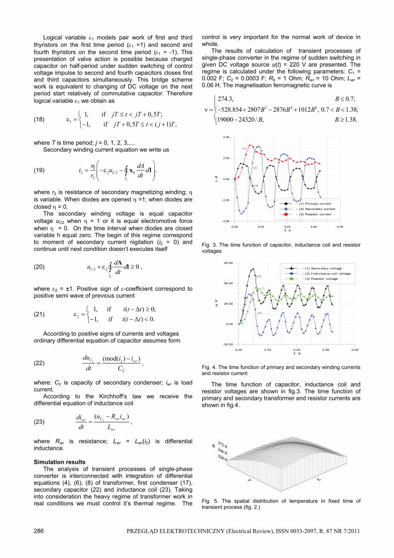
The results of calculation of transient processes of single-phase converter in the regime of sudden switching in given DC voltage source u(t) = 220 V are presented. The regime is calculated under the following parameters: C1 = 0.002 F; C2 = 0.0003 F; Rb = 1 Ohm; Rwr = 10 Ohm; Lwr = 0.06 H. The magnetisation ferromagnetic curve is

2 4 6

274.3, 0.7;

528.854 2807 2876 1012 , 0.7 1.38;

19000 24320/ , 1.38.

B

B B B B

B B

Fig. 3. The time function of capacitor, inductance coil and resistor voltages Fig. 4. The time function of primary and secondary winding currents and resistor current

The time function of capacitor, inductance coil and resistor voltages are shown in fig.3. The time function of primary and secondary transformer and resistor currents are shown in fig.4. Fig. 5. The spatial distribution of temperature in fixed time of transient process (fig. 2.)

0.00 0.02 0.04 0.06 0.08

t, s

-4.00

-2.00

0.00

2.00

4.00

i, A

- (1) Primary current

- (2) Secondary current

- (3) Resistor current

(1)

(3)

(2)

0.00 0.02 0.04 0.06 0.08

t, s

-20.00

0.00

20.00

40.00

60.00

u, V

- (1) Secondary voltage

- (2) Inductance coil voltage

- (3) Resistor voltage(1)

(3)

(2)

PRZEGLĄD ELEKTROTECHNICZNY (Electrical Review), ISSN 0033-2097, R. 87 NR 7/2011 287

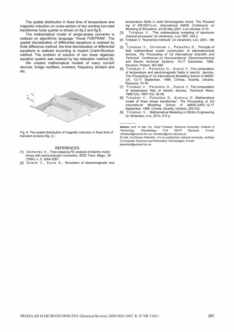
The spatial distribution in fixed time of temperature and magnetic induction on cross-section of two winding iron-clad transformer body quarter is shown on fig.5 and fig.6. The mathematical model of single-phase convertor is realized on algorithmic language ”Visual FORTRAN”. The spatial discretization of differential equations is realized by finite difference method; the time discretization of differential equations is realized according to implicit Crank-Nicolson method. The problem of solution of non linear algebraic equation system was realized by top relaxation method [5]. We created mathematical models of many convert devices: bridge rectifiers, inverters, frequency dividers and etc. Fig. 6. The spatial distribution of magnetic induction in fixed time of transient process (fig. 2.)

REFERENCES

[1] Demenko A . , Time stepping FE analysis of electric motor drives with semiconductor converters, IEEE Trans. Magn., 30 (1994), n. 5, 3264-3267.

[2] Dubuk V . , Kyc ia E . , Simulation of electromagnetic and

temperature fields in solid ferromagnetic toroid, The Proceed ing of MS’2001-Lviv, International AMSE Conference on Modeling & Simulation, 23-26 May 2001, Lviv-Ukraine, 9-10.

[3] Tchaban V . , “The mathematical modelling of electrome chanical processes” (in Ukrainian), Lviv,1997, 344 p.

[4] Tchaban V. “Numerical methods” (in Ukrainian), Lviv, 2001, 186 p.

[5] Tchaban V . , Chromiak J . , Pe leshko D . , Principle of field mathematical model construction of electrotechnical devices, The Proceeding of 1st International Scientific and Technical Conference on Unconventional Electromechanical and Electro technical Systems, 15-17 December, 1995, Szczecin, Poland, 363-366.

[6]. Tchaban V . , Pe leshko D . , Dubuk V ., The computation of temperature and electromagnetic fields in electric devices, The Proceeding of 1st International Modelling School of AMSE-UA, 12-17 September, 1996, Crimea, Alushta, Ukraine, Rzeszow, 75-78.

[7] Tchaban V . , Pe leshko D . , Dubuk V . The computation of temperature field of electric devices, Technical News, 1996/1(4), 1997/1(5), 56-58.

[8] Tchaban V . , Pe leshko D . , Ko lkovy O. Mathematical model of three phase transformer”, The Proceeding of 3rd International Modelling School of AMSE-UAPL,12-17 September, 1999, Crimea, Alushta, Ukraine, 229-232.

[9] Tchaban V . , Mathematical Modeling in Eltctric Engineering (in Ukrainian), Lviv, 2010, 510 p.

––––––––– Autors: prof. dr hab. Inz. Vasyl Tchaban, Rzeszow University, Institute of Technology, Pilsudskiego 21/4 35074 Rzeszow, E-mail: vtchaban@polynet.lviv.ua; vtchaban@univ.rzeszow.pl; Dr hab. Inz.Dmytro Peleshko of Lviv polytechnic national university, Institute of Computer Sciences and Infromation Technologies, E-mail: peleshko@polynet.lviv.ua