Comparison of an impulse and a reaction turbine stage for ...

archivesof thermodynamics

Vol. 40(2019), No. 3, 137–157

DOI: 10.24425/ather.2019.129998

Comparison of an impulse and a reaction turbine

stage for an ORC power plant

DAWID ZANIEWSKI∗

PIOTR KLIMASZEWSKIŁUKASZ WITANOWSKIŁUKASZ JEDRZEJEWSKIPIOTR KLONOWICZPIOTR LAMPART

Institute of Fluid Flow Machinery Polish Academy of Sciences, Centre ofHeat and Power Engineering, Turbine Department, Fiszera 14,80-231 Gdańsk, Poland

Abstract Turbine stages can be divided into two types: impulse stagesand reaction stages. The advantages of one type over the second one aregenerally known based on the basic physics of turbine stage. In this paperthese differences between mentioned two types of turbines were indicated onthe example of single stage turbines dedicated to work in organic Rankinecycle (ORC) power systems. The turbines for two ORC cases were analysed:the plant generating up to 30 kW and up to 300 kW of net electric power,respectively. Mentioned ORC systems operate with different working fluids:DMC (dimethyl carbonate) for the 30 kW power plant and MM (hexam-ethyldisiloxane) for the 300 kW power plant. The turbines were comparedaccording to three major issues: thermodynamic and aerodynamic perfor-mance, mechanical and manufacturing aspects. The analysis was performedby means of the 0D turbomachinery theory and 3D computational aerody-namic calculations. As a result of this analysis, the paper indicates conclu-sions which type of turbine is a recommended choice to use in ORC systemstaking into account the features of these systems.

Keywords: CFD; Waste heat recovery; Steam turbine; Organic Rankine cycle

∗Corresponding Author. Email: [email protected]

138 D. Zaniewski et al.

Nomenclature

b – chord of a profile, mmc – velocity in the stationary frame, m/scs – spouting velocity, m/sD/l – mean diameter related to the height of a bladel – height of a blade, mmLax – axial length of a blade, mmM – Mach numberPNET – net power produced by a turbine obtained making use of

0D theory, kWR – mean radius of a stator/rotor, mmRh – hub radius of a stator/rotor, mmRs – external radius of a stator/rotor, mmu – peripheral speed, m/sw – velocity in the rotating frame, m/sZ – quantity of blades of a rotor/stator

Greek symbols

α – angle of the stream in the stationary frame, ◦

β – angle of the stream in the rotating frame, ◦

ηETN – net isentropic efficiency obtained making use of0D theory,%

ηNET_CFD – net isentropic efficiency calculated making use of CFD, %Θh – degree of reaction at the hub, %△h – energy losses, kJ/kg

1 Introduction

In general turbines can be divided into two types: the impulse type whichhas the degree of reaction equal to 0 and the reaction type with the de-gree of reaction equal to 0.5. The degree of reaction can be described asa ratio of the isentropic enthalpy drop in a rotor to the isentropic enthalpydrop in the whole stage. This distinction has a historical meaning becausepresently turbines are usually designed with a degree of reaction between0 and 0.5 or sometimes even more than 0.5. The conventional distinctiondetermines the impulse turbines as machines with the degree of reactionbetween 0 and 0.3 and the reaction turbines as machines with the degreeof reaction greater than 0.3 up to 0.5 (or more) but anyway this distinctionhas a smooth boundary [1–3]. Because of a few principal differences, thesetwo types of machines have a different construction. It applies especiallyto axial turbines. Radial turbines (radial inflow and radial outflow) areusually designed as a reaction type [4–6] although there are designs with

Comparison of an impulse and a reaction turbine stage. . . 139

a low degree of reaction [7–10].Each type of turbine has specific advantages and disadvantages. In

general the comparison of these two types of machines should include thefollowing points:

• thermodynamic and aerodynamic performance,

• parameters of work which affect the construction of a machine,

• technological challenge during manufacturing of parts of the ma-chines.

A few advantages of one type over the second one are generally knownand based on the fundamental physics of turbines. These examples aredescribed below.

The impulse turbine accelerates gas mainly during expansion in nozzles.Because of that the absolute outlet velocity from the vane is much higherthan in the reaction turbine. It leads to greater losses during flow throughthe channel. Thus the impulse turbine efficiency potential is generally lowerthan that of the reaction turbine [1–3,11]. Because of expansion in the rotorof the reaction turbine there is a pressure difference between the rotorinlet and outlet. It leads to higher tip clearance losses for the reactionturbine than for the impulse one in case of an identical tip clearance [11].The mentioned pressure difference causes also the axial thrust which hasto be countered by the thrust bearing and sometimes has to be balancedusing the high pressure gas in the form of a so called relief piston [1,2,11].Another advantage of the impulse turbine over the reaction one is muchlower optimal peripheral speed, which is significantly lower for the identicalenthalpy drop. It leads to lower stress in rotating parts during the turbineoperation [3,4,11].

The paper presents analysis of two types of turbines: the axial impulsetype and the radial inflow reaction type. An analysis was done for turbinesdedicated to work in organic Rankine cycle (ORC). The first case considersan ORC system generating about 30 kW of electrical power which is workingwith DMC (dimethyl carbonate) fluid. The second case considers a powerplant generating about 300 kW of electrical power and working with MM(hexamethyldisiloxane) fluid.

The design calculations of mentioned turbines were performed by meansof 0D theory (zero dimensional preliminary stage flow calculations) [1,2] anddetailed analysis was done through computational fluid dynamics [12] usingcommercial engineering simulation software Ansys CFX [13]. The purpose


of the analysis is to compare the radial and the axial turbine for the specificapplication mentioned above.

2 Turbine stage calculations

2.1 Boundary conditions

The boundary conditions for the 0D and the 3D fluid flow analysis wereobtained from the ORC heat balance calculation. The following parame-ters were used: inlet total pressure, inlet total temperature, outlet staticpressure and nominal rotational speed. For 0D analysis the value of massflow rate was also included. The analysed cases were ordered as follows:

• Case 1. The ORC plant with the DMC as working fluid – net powerequal to about 30 kWel:

⊲ A – axial impulse turbine with a low degree of reaction,

⊲ B – axial impulse turbine with a considerable degree of reaction,

⊲ C – radial inflow reaction turbine.

• Case 2. The ORC plant with the MM fluid – net nominal power upto 300 kWel:

⊲ A – axial impulse turbine with a considerable degree of reaction,

⊲ B – radial inflow reaction turbine.

The values of the boundary parameters for all cases are shown in Tab. 1.

Table 1: Values of the boundary parameters of the all analysed cases.

Parameters Case 1. Case 2.

Boundary parameters A B C A B

Degree of reaction in the mean radius [%] 9.3 25.2 49.5 27.6 50.0

Opt. rotational speed of rotor [rpm] 40000 41000 51555 14500 11000

Inlet total pressure [kPa] (abs) 1500 1026

Inlet total temperature [◦C] 211.2 210.47

Outlet static pressure [kPa] (abs) 23 21

Mass flow rate [kg/s] 0.396 5.759

Isentropic enthalpy drop [kJ/kg] 152.6 82.52


2.2 0D turbine theory

The 0D theory of turbomachinery which was used is the well-known methodof preliminary design of turbine stages. It allows a designer to shape theinitial geometry of the blades and the channel. This theory is usuallyenriched by additional empirical correlations for different kind of losseswhich could occur during flow through the channel so that the calculationresults become more realistic [14]. Basically the 0D theory is based onEuler’s turbomachinery equation, the continuity equation and the law ofconservation of energy [1–3]. Additionally, loss correlations were used [15].

The profiles shape was generated making use of the in-house softwarewhich is based on the 0D theory results and the commercial software AnsysBladeGen [16].

2.3 CFD analysis setup

The computational fluid dynamics (CFD) analysis was performed as a steadystate with the multiply frame of reference interface (‘frozen rotor’) betweenthe stator and rotor domains. The shroud, hub and blade surfaces weredefined as non-slip adiabatic smooth walls. The periodic boundary wereused as single blade channels were modelled. The tip clearance was notincluded in the analysis. The turbulence model used in the analysis wask-ω shear stress transport (SST).

3 Results of the analysis and conclusions

3.1 Case 1 – up to 30 kW ORC plant with DMC fluid

In the first step the axial impulse turbine with a low degree of reaction(Tabs. 2, 5, 6, and Figs. 1, 4, 5) and with a higher degree of reaction(Tabs. 3, 7, 8, and Figs. 2, 6, 7) are compared for the first case: A and B.For Case 1A the degree of reaction in the mean radius is 9.3% and this leadsto the negative degree of reaction at the hub. Situation like this usuallycauses the separation of the fluid at the hub which leads to additional loss.The turbine from Case 1B has the mean degree of reaction equal to 25.2%.This value is big enough to receive the positive value of this parameter atthe hub.

As it was mentioned before the impulse turbine will achieve a muchhigher outlet velocity from the nozzle (Figs. 4 and 6) for the same total


enthalpy drop. For Case 1A the value of this parameter is by 16% greaterthan it is for Case 1B. This fact and the mentioned problems with a neg-ative degree of reaction at the rotor hub yield lower isentropic efficiency(total to static) of the impulse turbine – 3.2 percent points lower than it isfor the other turbine.

In Case 1C (the radial inflow reaction turbine) all the calculations re-sults are presented in Tabs. 4, 9, 10 and Figs. 3, 8, 9. In this case with themean degree of reaction equal to 50% the outlet velocity from the nozzleis almost 30% lower than that in Case 1A – impulse axial turbine (Figs. 4and 8). It is one of the major reasons that the isentropic efficiency of thisturbine achieves 85.3% (Tab. 10) which is 8.5 percent point more than forthe impulse turbine with a low degree of reaction and 5.3 percent pointmore than for the other impulse turbine with a considerable degree of reac-tion. The impulse turbine has the lower isentropic efficiency also becauseof a relatively higher flow turning angle in the rotor channel which is thereason of additional profile loss and endwall loss. Another reason for thehigh isentropic efficiency of the radial reaction turbine is the attribute ofthe radial stage which is more efficient than axial impulse stage accordingto Euler’s equation. It is the reason why the axial impulse stage and theradial reaction stage could not easily be compared.

Case 1A and 1B have almost equal optimal rotational velocities (40 000and 41 000 rpm, respectively, Tab. 1). Case 1B has a higher value of pe-ripheral speed which yields greater dimensions of turbine wheels (Tab. 2,Fig. 1 and Tab. 3, Fig. 2) for the optimal design velocity ratio. A directconsequence of that is greater design challenge from the mechanical pointof view.

The optimal rotational speed of the turbine in Case 1C is higher thanthat in Cases 1A and 1B (Tab. 1). It leads to more problems with rotor-dynamic and structural aspects of the machine. The diameter of the rotorin the nozzle outlet control section is similar to that from case 1B (Tab. 3,Fig. 2 and Tab. 4, Fig. 3). It means that in conjunction with a greaterrotational speed this type of turbine will feature a higher peripheral speed.The 50% degree of reaction leads also to a relatively high pressure dropduring flow through the rotor, so for the similar diameters of rotors fromCase 1B and Case 1C the second one will receive much more axial thrust.All of these aspects are the reasons why the radial inflow reaction turbineis more difficult to design, also because of much more demanding shape ofthe rotor which is more difficult to manufacture.


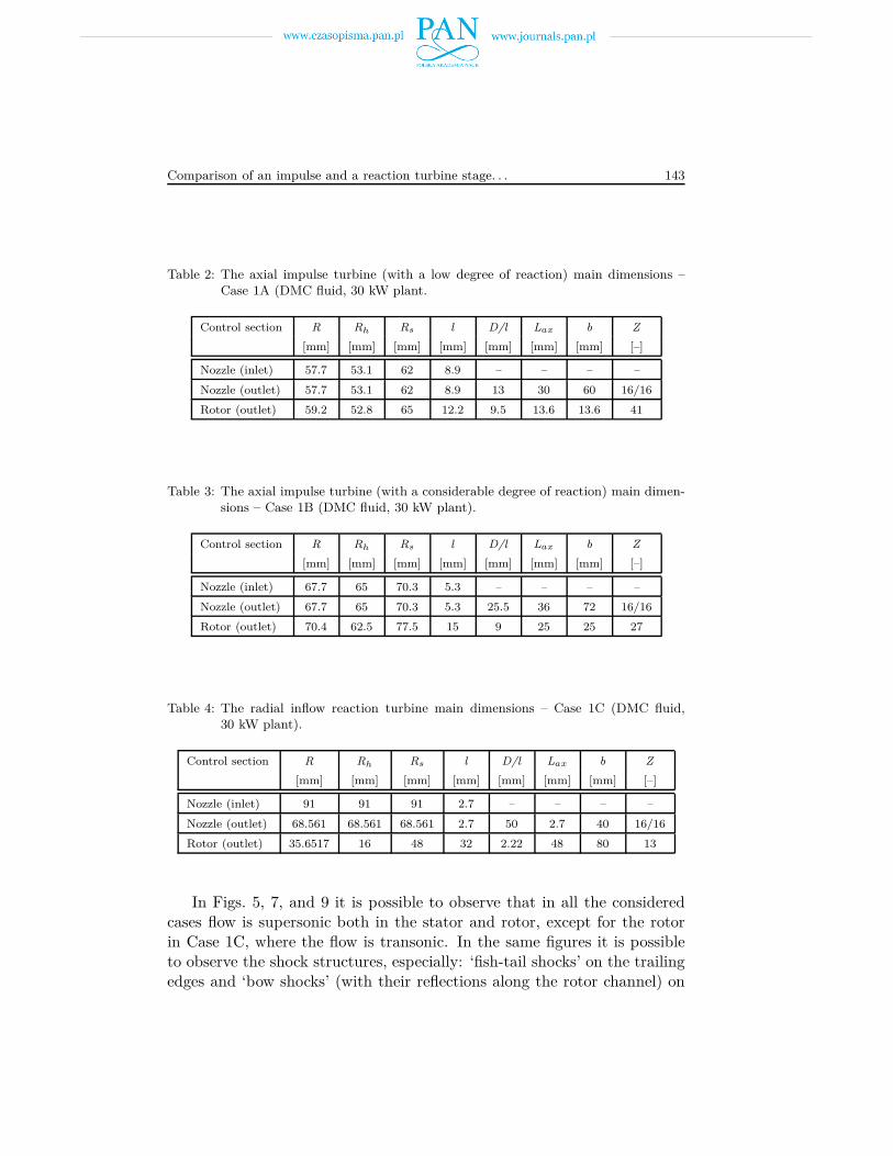
Table 2: The axial impulse turbine (with a low degree of reaction) main dimensions –Case 1A (DMC fluid, 30 kW plant.

Control section R Rh Rs l D/l Lax b Z

[mm] [mm] [mm] [mm] [mm] [mm] [mm] [–]

Nozzle (inlet) 57.7 53.1 62 8.9 – – – –

Nozzle (outlet) 57.7 53.1 62 8.9 13 30 60 16/16

Rotor (outlet) 59.2 52.8 65 12.2 9.5 13.6 13.6 41

Table 3: The axial impulse turbine (with a considerable degree of reaction) main dimen-sions – Case 1B (DMC fluid, 30 kW plant).


[mm] [mm] [mm] [mm] [mm] [mm] [mm] [–]

Nozzle (inlet) 67.7 65 70.3 5.3 – – – –

Nozzle (outlet) 67.7 65 70.3 5.3 25.5 36 72 16/16

Rotor (outlet) 70.4 62.5 77.5 15 9 25 25 27

Table 4: The radial inflow reaction turbine main dimensions – Case 1C (DMC fluid,30 kW plant).


[mm] [mm] [mm] [mm] [mm] [mm] [mm] [–]

Nozzle (inlet) 91 91 91 2.7 – – – –

Nozzle (outlet) 68.561 68.561 68.561 2.7 50 2.7 40 16/16

Rotor (outlet) 35.6517 16 48 32 2.22 48 80 13

In Figs. 5, 7, and 9 it is possible to observe that in all the consideredcases flow is supersonic both in the stator and rotor, except for the rotorin Case 1C, where the flow is transonic. In the same figures it is possibleto observe the shock structures, especially: ‘fish-tail shocks’ on the trailingedges and ‘bow shocks’ (with their reflections along the rotor channel) on


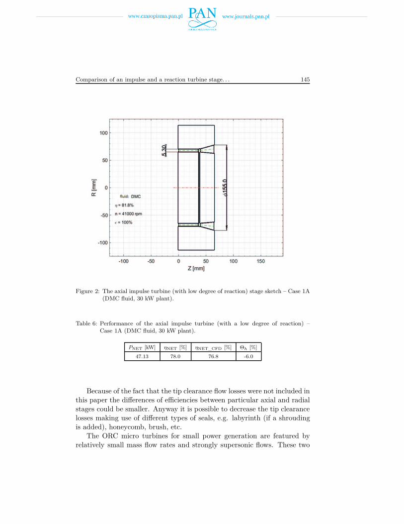
Figure 1: The axial impulse turbine (with low degree of reaction) stage sketch – Case 1A(DMC fluid, 30 kW plant).

Table 5: Kinematics values of the mean stream – Case 1A (DMC fluid, 30 kW plant).

Control section c w u α β M ∆hs u/cs

[m/s] [m/s] [m/s] [◦] [◦] [–] [kJ/kg] [–]

Nozzle (outlet) 499.16 271.86 241.67 14.43 27.22 2.580 13.84 0.45

Rotor I (outlet) 134.61 290.37 248.04 94.01 152.45 1.503 10.54 0.45

the leading edges of the rotor. In Case 1C it is difficult to observe anyshockwaves in the rotor region. It is very important that the observedshockwaves are relatively weak, therefore they are not the major part offlow losses. It has to be kept in mind that the shockwaves structures haveunsteady character and cannot be analysed properly in the case of steadystate analysis.


Figure 2: The axial impulse turbine (with low degree of reaction) stage sketch – Case 1A(DMC fluid, 30 kW plant).

Table 6: Performance of the axial impulse turbine (with a low degree of reaction) –Case 1A (DMC fluid, 30 kW plant).

PNET [kW] ηNET [%] ηNET_CFD [%] Θh [%]

47.13 78.0 76.8 -6.0

Because of the fact that the tip clearance flow losses were not included inthis paper the differences of efficiencies between particular axial and radialstages could be smaller. Anyway it is possible to decrease the tip clearancelosses making use of different types of seals, e.g. labyrinth (if a shroudingis added), honeycomb, brush, etc.

The ORC micro turbines for small power generation are featured byrelatively small mass flow rates and strongly supersonic flows. These two


Figure 3: The radial inflow reaction turbine stage sketch – Case 1C (DMC fluid, 30 kWplant).

Table 7: Kinematics values of the mean stream – Case 1B (DMC fluid, 30 kW plant).


[m/s] [m/s] [m/s] [◦] [◦] [–] [kJ/kg] [–]

Nozzle (outlet) 453.4 178.57 290.68 11.63 30.78 2.312 11.42 0.55

Rotor I (outlet) 92.44 304.05 302.27 82.32 162.46 1.576 11.56 0.55

Table 8: Performance of the axial impulse turbine (with considerable degree of reaction)– Case 1B (DMC fluid, 30 kW plant).


49.43 81.8 80.0 19.0

aspects lead to the fact that a turbine nozzle has to be designed as a deLaval nozzle with very small critical section which means that the throat be-tween the blades can be even less than 1 mm (e.g. turbines from Cases 1A,


Table 9: Kinematics values of the mean stream – Case 1C (DMC fluid, 30 kW plant).


[m/s] [m/s] [m/s] [◦] [◦] [–] [kJ/kg] [–]

Nozzle (outlet) 376.45 65.37 370.15 10 89.49 1.90 6.10 0.67

Rotor I (outlet) 91.568 215.90 192.48 91.92 154.92 1.13 5.27 0.67

Table 10: Performance of the radial inflow reaction turbine – Case 1C (DMC fluid,30 kW plant).

P NET [kW] ηNET [%] ηNET_CFD [%]

54.6 90.3 85.3

Figure 4: Velocity vectors at the mean diameter of the axial impulse turbine (with lowdegree of reaction) – Case 1A (DMC fluid, 30 kW plant).

1B and 1C). Such channels can be extremely difficult to manufacture (withacceptable tolerances) what is the reason why nozzles of those turbines haveto be specially shaped (contoured) through the meridional section as well.


Figure 5: Mach Number contours (left side) and pressure gradient contours (right side)at the mean diameter of the axial impulse turbine (with low degree of reaction)– Case 1A (DMC fluid, 30 kW plant).

Figure 6: Velocity vectors at the mean diameter of the axial impulse turbine (with con-siderable degree of reaction) – Case 1B (DMC fluid, 30 kW plant).

The considered ORC turbine will be part of a hermetic micro turbo-generator characterised by a compact construction. Because of that it isvery important to prepare a design which is a compromise between small


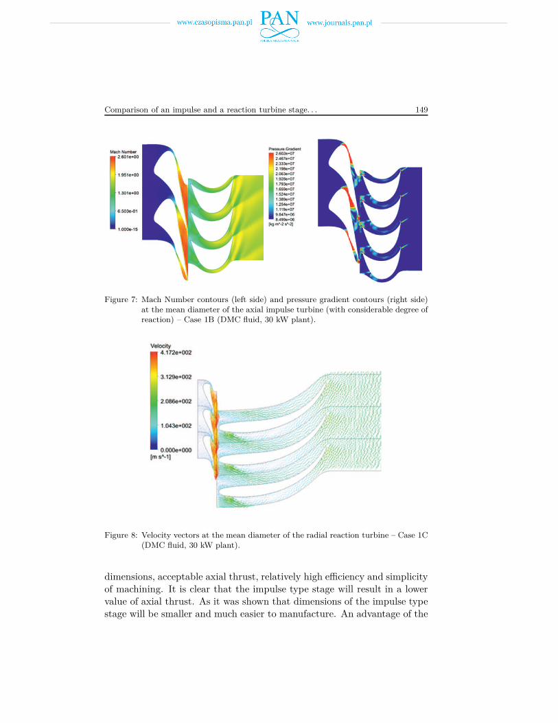
Figure 7: Mach Number contours (left side) and pressure gradient contours (right side)at the mean diameter of the axial impulse turbine (with considerable degree ofreaction) – Case 1B (DMC fluid, 30 kW plant).

Figure 8: Velocity vectors at the mean diameter of the radial reaction turbine – Case 1C(DMC fluid, 30 kW plant).

dimensions, acceptable axial thrust, relatively high efficiency and simplicityof machining. It is clear that the impulse type stage will result in a lowervalue of axial thrust. As it was shown that dimensions of the impulse typestage will be smaller and much easier to manufacture. An advantage of the


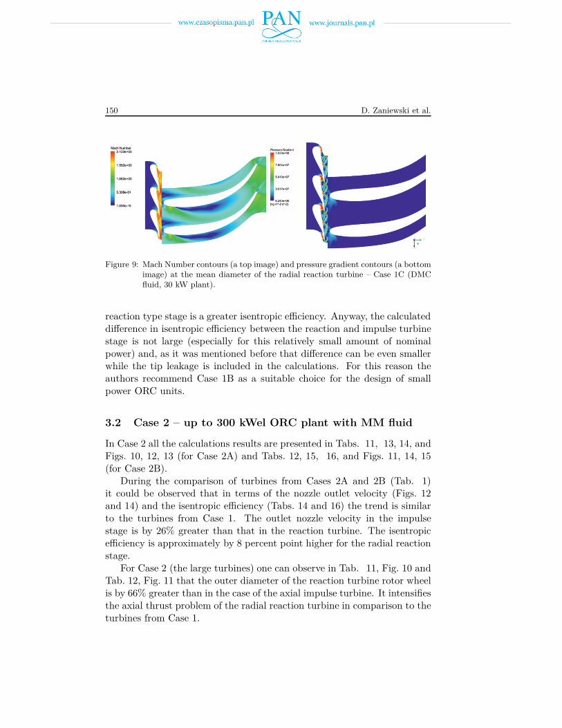
Figure 9: Mach Number contours (a top image) and pressure gradient contours (a bottomimage) at the mean diameter of the radial reaction turbine – Case 1C (DMCfluid, 30 kW plant).

reaction type stage is a greater isentropic efficiency. Anyway, the calculateddifference in isentropic efficiency between the reaction and impulse turbinestage is not large (especially for this relatively small amount of nominalpower) and, as it was mentioned before that difference can be even smallerwhile the tip leakage is included in the calculations. For this reason theauthors recommend Case 1B as a suitable choice for the design of smallpower ORC units.

3.2 Case 2 – up to 300 kWel ORC plant with MM fluid

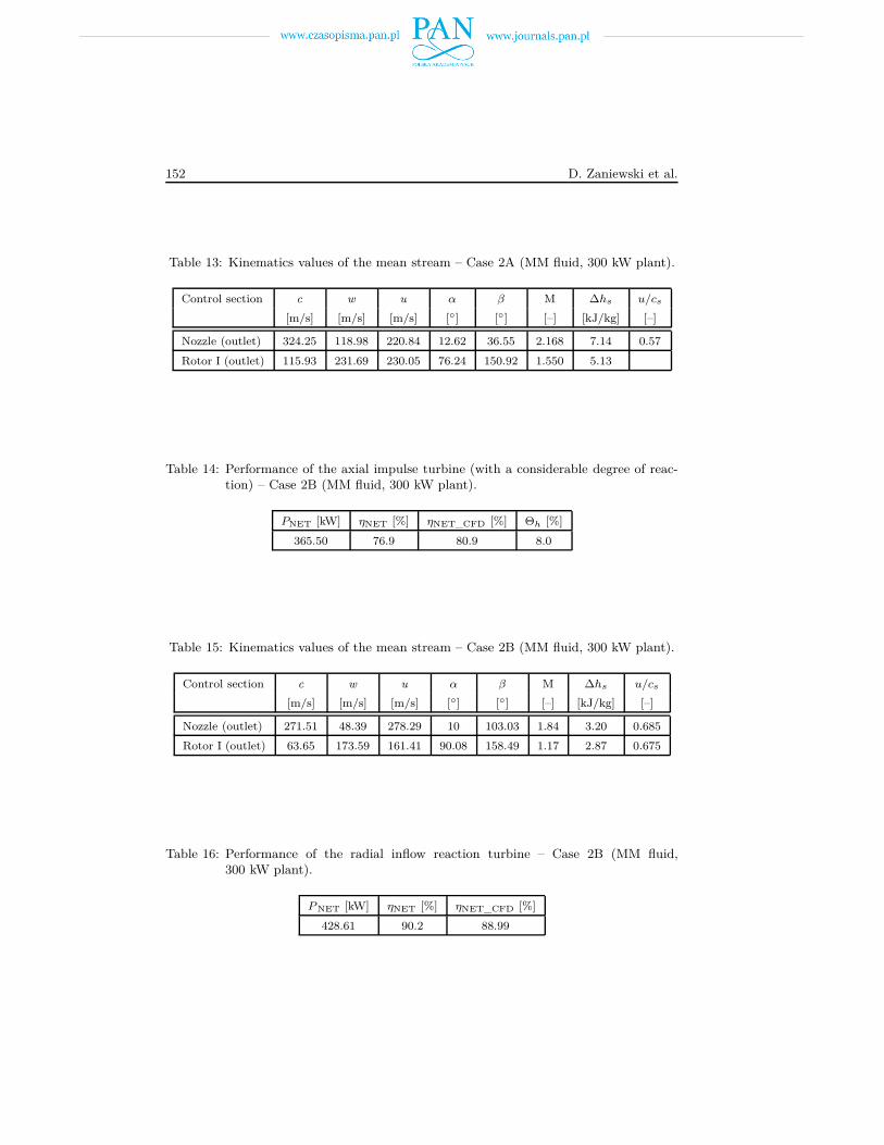
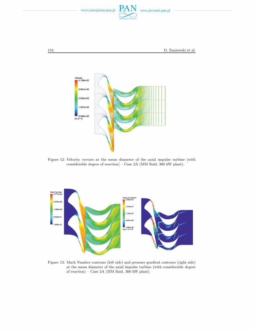
In Case 2 all the calculations results are presented in Tabs. 11, 13, 14, andFigs. 10, 12, 13 (for Case 2A) and Tabs. 12, 15, 16, and Figs. 11, 14, 15(for Case 2B).

During the comparison of turbines from Cases 2A and 2B (Tab. 1)it could be observed that in terms of the nozzle outlet velocity (Figs. 12and 14) and the isentropic efficiency (Tabs. 14 and 16) the trend is similarto the turbines from Case 1. The outlet nozzle velocity in the impulsestage is by 26% greater than that in the reaction turbine. The isentropicefficiency is approximately by 8 percent point higher for the radial reactionstage.

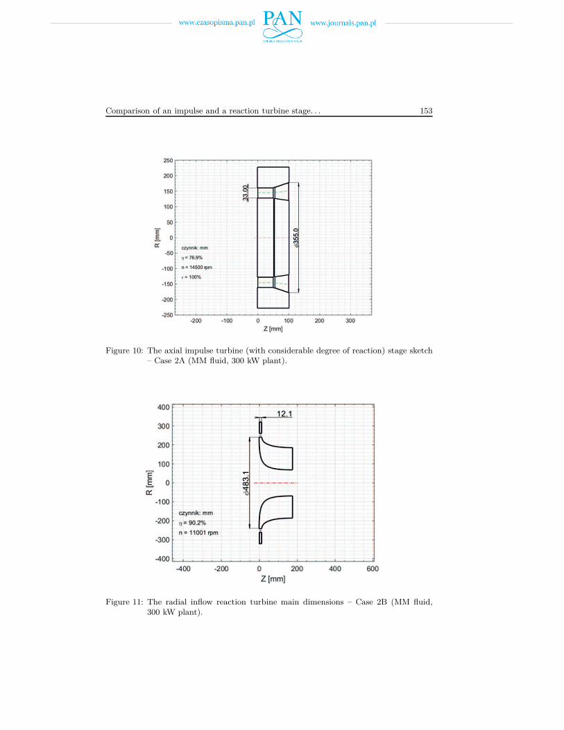
For Case 2 (the large turbines) one can observe in Tab. 11, Fig. 10 andTab. 12, Fig. 11 that the outer diameter of the reaction turbine rotor wheelis by 66% greater than in the case of the axial impulse turbine. It intensifiesthe axial thrust problem of the radial reaction turbine in comparison to theturbines from Case 1.


The optimal rotational speed is 25% smaller for the radial reaction stage(Case 2B) than in the case of axial impulse stage (Case 2A). Anyway muchgreater dimensions of the rotor probably will cause more problems withrotordynamic aspects of a machine.

As it was in the Case 1 also in Case 2 the flow is supersonic in both thestator and rotor of the axial impulse turbine with a considerable degree ofreaction. In the case of the radial-axial inflow turbine the flow is supersonicin the stator, but transonic in the rotor. Shockwaves structures are alsosimilar to those described in Case 1.

The turbines which generate a relatively higher power (like these fromCases 2A and 2B, Tab. 3.1), usually do not cause the problems with thenozzle throat to the extent like that mentioned above because of the highermass flow rate. For the same reason which is described in the chapter 3.1the authors decide to choose the Case 2A as a target type of the turbineconstruction. Anyway in this case it has to be mentioned that the totalgenerated power is much greater than it is in the Case 1, so the differencein the amount of isentropic efficiency between the cases: 2A and 2B is moreimportant.

Table 11: The axial impulse turbine (with a considerable degree of reaction) main di-mensions – Case 2A (MM fluid, 300 kW plant).


[mm] [mm] [mm] [mm] [mm] [mm] [mm] [–]

Nozzle (outlet) 145.4 128.0 161.0 33.0 8.8 50.0 122.3 20/20

Rotor (outlet) 151.5 120.0 177.5 57.5 5.1 45.0 46.1 31

Table 12: The radial inflow reaction turbine main dimensions – Case 2B (MM fluid,300 kW plant).


[mm] [mm] [mm] [mm] [mm] [mm] [mm] [–]

Nozzle (outlet) 241.6 241.6 241.6 12.1 40.0 12.1 60.4 32/32

Rotor (outlet) 140.1 69.0 150.0 116.8 2.40 176.4 294.5 11


Table 13: Kinematics values of the mean stream – Case 2A (MM fluid, 300 kW plant).


[m/s] [m/s] [m/s] [◦] [◦] [–] [kJ/kg] [–]

Nozzle (outlet) 324.25 118.98 220.84 12.62 36.55 2.168 7.14 0.57

Rotor I (outlet) 115.93 231.69 230.05 76.24 150.92 1.550 5.13

Table 14: Performance of the axial impulse turbine (with a considerable degree of reac-tion) – Case 2B (MM fluid, 300 kW plant).


365.50 76.9 80.9 8.0

Table 15: Kinematics values of the mean stream – Case 2B (MM fluid, 300 kW plant).


[m/s] [m/s] [m/s] [◦] [◦] [–] [kJ/kg] [–]

Nozzle (outlet) 271.51 48.39 278.29 10 103.03 1.84 3.20 0.685

Rotor I (outlet) 63.65 173.59 161.41 90.08 158.49 1.17 2.87 0.675

Table 16: Performance of the radial inflow reaction turbine – Case 2B (MM fluid,300 kW plant).

P NET [kW] ηNET [%] ηNET_CFD [%]

428.61 90.2 88.99


Figure 10: The axial impulse turbine (with considerable degree of reaction) stage sketch– Case 2A (MM fluid, 300 kW plant).

Figure 11: The radial inflow reaction turbine main dimensions – Case 2B (MM fluid,300 kW plant).


Figure 12: Velocity vectors at the mean diameter of the axial impulse turbine (withconsiderable degree of reaction) – Case 2A (MM fluid, 300 kW plant).

Figure 13: Mach Number contours (left side) and pressure gradient contours (right side)at the mean diameter of the axial impulse turbine (with considerable degreeof reaction) – Case 2A (MM fluid, 300 kW plant).


Figure 14: Velocity vectors at the mean diameter of the radial reaction turbine – Case 2B(MM fluid, 300 kW plant).

Figure 15: Mach Number contours (left side) and pressure gradient contours (right side)at the mean diameter of the radial reaction turbine – Case 2B (MM fluid,300 kW plant).


4 Summary

A number of ORC turbine designs including impulse-type and radial-typeturbines have been analysed in the paper from the point of view of flowefficiency, mechanical and machining aspects. It follows from the analysis ofresults presented in the paper that for ORC power plants, especially micropower plants, the suitable choice of a turbine is the axial impulse turbinewith a considerable degree of reaction (about 25% at the mean radius). It isa compromise between small dimensions, acceptable axial thrust, relativelyhigh efficiency and simplicity of machining. This compromise provides thatthis type of turbine can be recommended to use as a part of a compact andhermetic micro turbogenerator for ORC power plant whose main goal isusually to generate the maximum possible power not necessarily with thehighest efficiency.

Acknowledgements This work has been partially founded by by TheNational Centre for Research and Development and by The Smart GrowthOperational Programme (European funds) within the project No. POIR.01.01.01-00-0414/17 and POIR.01.01.01-00-0512/16 carried out jointly withthe Marani Company. Calculations were carried out at the Academic Com-puter Centre in Gdańsk.

Received 12 December 2018

References

[1] Perycz S.: Steam and Gas Turbines. Ossolineum, Wrocław Warszawa Kraków 1992(in Polish).

[2] Japikse D., Baines N.C.: Introduction to Turbomachinery. Concepts ETI, 1994.

[3] Dixon S.L.: Fluid Mechanics and Themodynamics of Turbomachinery (5th Edn.).Pergamon Press, 2005.

[4] Fiaschi D., Manfrida G., Maraschiello F.: Thermo-fluid dynamics preliminarydesign of turbo-expanders for ORC cycles. Appl. Energ.. 97(2012), 601–608.

[5] Pini M., Perisco G., Casati E., Dossena V.: Preliminary design of a centrifugalturbine for ORC applications. In: Proc. 1st Int. Sem. on ORC Power Systems ORC2011, Delft 2011.

[6] Spadacini C., Rizzi D., Saccilotto C., Salgorollo S., Centemeri L.: Theradial outflow turbine technology. In: Proc. 2nd Int. Sem. on ORC Power SystemsASME ORC 2013, Rotterdam 2013.


[7] Harinck J., Pasquale D., Pecnik R., van Buijtenen J., Colonna L.: Per-formance improvement of a radial organic Rankine cycle turbine by means of au-tomated computational fluid dynamic design. Proc. Inst. Mech. Eng. A J. PowerEnergy 227(2013), 637–645.

[8] Klonowicz P., Bröggemann D.: 2D unsteady RANS simulations of an organicvapor partial admission turbine. In: Proc. 2nd Int. Sem. on ORC Power SystemsASME ORC 2013, Rotterdam 2013.

[9] Kiciński J., Żywica G.: Steam Microturbines in Distributed Cogeneration.Springer International Publishing, 2014.

[10] Weiss A.P., Popp T., Müller J., Brüggemann , Preissinger M.: Experimentalcharacterization and comparison of an axial and a cantilever micro-turbine for small-scale Organic Rankine Cycle, Appl. Therm. Eng. 140(2018), 235–244.

[11] Weiss A.P.: Volumetric expanders versus turbine – which is the better choice forsmall ORC plants? In: Proc. 3rd Int. Sem. on ORC Power Systems, Brussels 2015.

[12] Klonowicz P., Hanausek P.: Optimum design of the axial ORC turbines withsupport of the Ansys CFX flow. In: Proc. 1st Int. Sem. on ORC Power SystemsORC 2011, Delft 2011.

[13] Ansys Academic Research CFX, Release 19.1.

[14] Klonowicz P., Heberle F., Preissinger M., Brüggemann D.: Significanceof loss correaltions in performance prediction of small scale, highly loaded turbinestages working in Organic Rankine Cycles. Energy 72(2014), 322–330.

[15] Traupel W.: Thermische Turbomaschinen. Springer Singapore Pte., 2001.

[16] Ansys Academic BladeGen, Release 19.1.

[17] Kosowski K., Piwowarski M., Stepień R., Włodarski W.: Design and inves-tigations of the ethanol microturbine. Arch. Thermodyn. 39(2018), 2, 41–54.

[18] Wajs J., Mikielewicz D., Bajor M., Kneba Z.: Experimental investigation ofdomestic micro-CHP based on the gas boiler fitted with ORC module. Arch. Ther-modyn. 37(2016), 3, 79–93.

Comparison of an impulse and a reaction turbine stage for ...

Documents

Transcript of Comparison of an impulse and a reaction turbine stage for ...