
Chap2 Modeling
32
Chapter 2: Modeling Concepts 1 CHAPTER 2 MODELING CONCEPTS 1 Introduction As was discussed in the previous chapter, in order to apply optimization methods we must have a model to optimize. As we also mentioned, obtaining a good model of the design problem is the most important step in optimization. In this chapter we discuss some modeling concepts that can help you develop models which can successfully be optimized. We also discuss the formulation of objectives and constraints for some special situations. We look at how graphics can help us understand the nature of the design space and the model. We end with an example optimization of a heat pump. 2 Physical Models vs. Experimental Models Two types of models are often used with optimization methods: physical models and experimental models. Physical models are based on the underlying physical principles that govern the problem. Experimental models are based on models of experimental data. Some models contain both physical and experimental elements. We will discuss both types of models briefly. 2.1 Physical Models Physical models can be either analytical or numerical in nature. For example, the Two-bar truss is an analytical, physical model. The equations are based on modeling the physical phenomena of stress, buckling stress and deflection. The equations are all closed form, analytical expressions. If we used numerical methods, such as the finite element method, to solve for the solution to the model, we would have a numerical, physical model. 2.2 Experimental Models Experimental models are based on experimental data. A functional relationship for the data is proposed and fit to the data. If the fit is good, the model is retained; if not, a new relationship is used. For example if we wish to find the friction factor for a pipe, we could refer to the Moody chart, or use expressions based on a curve fit of the data. 3 Modeling Considerations 3.1 Making the Model Robust During optimization, the algorithms will move through the design space seeking an optimum. Sometimes the algorithms will generate unanticipated designs during this process. To have a successful optimization, the model must be able to handle these designs, i.e. it must be robust. Before optimizing, you should consider if there are there any designs for which the model is undefined. If such designs exist, you need to take steps to insure either that 1) the optimization problem is defined such that the model will never see these designs, or 2) the model is made “bulletproof” so it can survive these designs.
-
Upload
aarulmurugu5005 -
Category
Documents
-
view
247 -
download
0
Transcript of Chap2 Modeling
Chapter 2: Modeling Concepts
1
CHAPTER 2
MODELING CONCEPTS
1 Introduction
As was discussed in the previous chapter, in order to apply optimization methods we must have a model to optimize. As we also mentioned, obtaining a good model of the design problem is the most important step in optimization. In this chapter we discuss some modeling concepts that can help you develop models which can successfully be optimized. We also discuss the formulation of objectives and constraints for some special situations. We look at how graphics can help us understand the nature of the design space and the model. We end with an example optimization of a heat pump.
2 Physical Models vs. Experimental Models
Two types of models are often used with optimization methods: physical models and experimental models. Physical models are based on the underlying physical principles that govern the problem. Experimental models are based on models of experimental data. Some models contain both physical and experimental elements. We will discuss both types of models briefly.
2.1 Physical Models
Physical models can be either analytical or numerical in nature. For example, the Two-bar truss is an analytical, physical model. The equations are based on modeling the physical phenomena of stress, buckling stress and deflection. The equations are all closed form, analytical expressions. If we used numerical methods, such as the finite element method, to solve for the solution to the model, we would have a numerical, physical model.
2.2 Experimental Models
Experimental models are based on experimental data. A functional relationship for the data is proposed and fit to the data. If the fit is good, the model is retained; if not, a new relationship is used. For example if we wish to find the friction factor for a pipe, we could refer to the Moody chart, or use expressions based on a curve fit of the data.
3 Modeling Considerations
3.1 Making the Model Robust
During optimization, the algorithms will move through the design space seeking an optimum. Sometimes the algorithms will generate unanticipated designs during this process. To have a successful optimization, the model must be able to handle these designs, i.e. it must be robust. Before optimizing, you should consider if there are there any designs for which the model is undefined. If such designs exist, you need to take steps to insure either that 1) the optimization problem is defined such that the model will never see these designs, or 2) the model is made “bulletproof” so it can survive these designs.
Chapter 2: Modeling Concepts
2
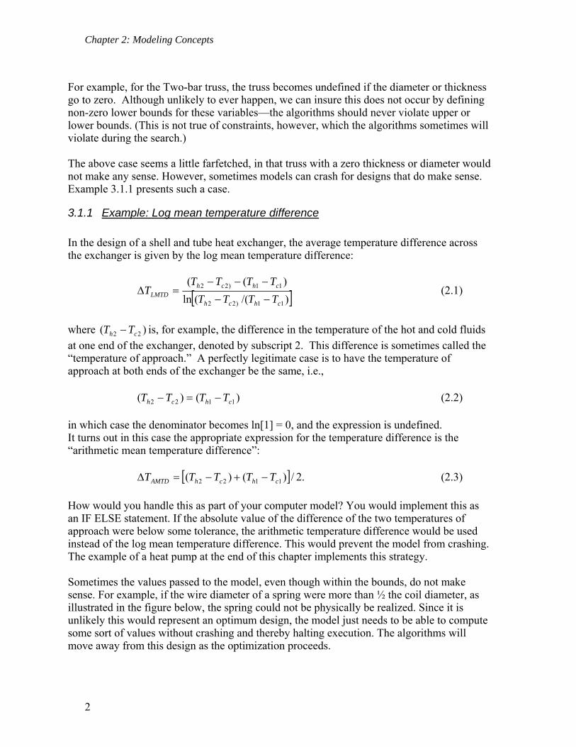
For example, for the Two-bar truss, the truss becomes undefined if the diameter or thickness go to zero. Although unlikely to ever happen, we can insure this does not occur by defining non-zero lower bounds for these variables—the algorithms should never violate upper or lower bounds. (This is not true of constraints, however, which the algorithms sometimes will violate during the search.) The above case seems a little farfetched, in that truss with a zero thickness or diameter would not make any sense. However, sometimes models can crash for designs that do make sense. Example 3.1.1 presents such a case.
3.1.1 Example: Log mean temperature difference
In the design of a shell and tube heat exchanger, the average temperature difference across the exchanger is given by the log mean temperature difference:
)/((ln
)((
11)22
11)22
chch
chchLMTD TTTT
TTTTT
(2.1)
where )( 22 ch TT is, for example, the difference in the temperature of the hot and cold fluids
at one end of the exchanger, denoted by subscript 2. This difference is sometimes called the “temperature of approach.” A perfectly legitimate case is to have the temperature of approach at both ends of the exchanger be the same, i.e., )()( 1122 chch TTTT (2.2) in which case the denominator becomes ln[1] = 0, and the expression is undefined. It turns out in this case the appropriate expression for the temperature difference is the “arithmetic mean temperature difference”: .2/)()( 1122 chchAMTD TTTTT (2.3)
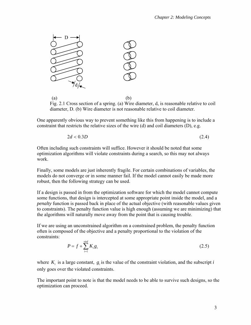
How would you handle this as part of your computer model? You would implement this as an IF ELSE statement. If the absolute value of the difference of the two temperatures of approach were below some tolerance, the arithmetic temperature difference would be used instead of the log mean temperature difference. This would prevent the model from crashing. The example of a heat pump at the end of this chapter implements this strategy. Sometimes the values passed to the model, even though within the bounds, do not make sense. For example, if the wire diameter of a spring were more than ½ the coil diameter, as illustrated in the figure below, the spring could not be physically be realized. Since it is unlikely this would represent an optimum design, the model just needs to be able to compute some sort of values without crashing and thereby halting execution. The algorithms will move away from this design as the optimization proceeds.
Chapter 2: Modeling Concepts
3
(a) (b)
Fig. 2.1 Cross section of a spring. (a) Wire diameter, d, is reasonable relative to coil diameter, D. (b) Wire diameter is not reasonable relative to coil diameter.
One apparently obvious way to prevent something like this from happening is to include a constraint that restricts the relative sizes of the wire (d) and coil diameters (D), e.g. Dd 3.02 (2.4) Often including such constraints will suffice. However it should be noted that some optimization algorithms will violate constraints during a search, so this may not always work. Finally, some models are just inherently fragile. For certain combinations of variables, the models do not converge or in some manner fail. If the model cannot easily be made more robust, then the following strategy can be used. If a design is passed in from the optimization software for which the model cannot compute some functions, that design is intercepted at some appropriate point inside the model, and a penalty function is passed back in place of the actual objective (with reasonable values given to constraints). The penalty function value is high enough (assuming we are minimizing) that the algorithms will naturally move away from the point that is causing trouble. If we are using an unconstrained algorithm on a constrained problem, the penalty function often is composed of the objective and a penalty proportional to the violation of the constraints:
1
viol
i ii
P f K g
(2.5)
where iK is a large constant, ig is the value of the constraint violation, and the subscript i
only goes over the violated constraints. The important point to note is that the model needs to be able to survive such designs, so the optimization can proceed.
D
d
Chapter 2: Modeling Concepts
4
3.2 Making Sure the Model is Adequate
Engineering models always involve assumptions and simplifications. An engineering model should be as simple as possible, but no simpler. If the model is not adequate, i.e., does not contain all of the necessary physics, the optimization routines will often exploit the inadequacy in order to achieve a better optimum. Obviously such an optimum does not represent reality. For example, in the past, students have optimized the design of a bicycle frame. The objective was to minimize weight subject to constraints on stress and column buckling. The optimized design looked like it was made of pop cans: the frame consisted of large diameter, very thin wall tubes. The design satisfied all the given constraints. The problem, however, was that the model was not adequate, in that it did not consider local buckling (the type of buckling which occurs when a pop can is crushed). For the design to be realistic, it needed to include local buckling. Another example concerns thermal systems. If the Second Law of Thermodynamics is not included in the model, the algorithms might take advantage of this to find a better optimum (you can achieve some wonderful results if the Second Law doesn’t have to be obeyed!). For example, I have seen optimal solutions which were excellent because heat could flow “uphill,” i.e. against a temperature gradient.
3.3 Testing the Model Thoroughly
The previous two sections highlight the need for a model which will be optimized to be tested thoroughly. The model should first be tested at several points for which solutions (at least “ballpark solutions”) are known. The model should then be exercised and pushed more to its limits to see where possible problems might lie.
3.4 Reducing Numerical Noise
Many engineering models are noisy. Noise refers to a lack of significant figures in the function values. Noise often results when approximation techniques or numerical methods are used to obtain a solution. For example, the accuracy of finite element methods depends on the “goodness” of the underlying mesh. Models that involve finite difference methods, numerical integration, or solution of sets of nonlinear equations all contain noise to some degree. It is important that you recognize that noise may exist. Noise can cause a number of problems, but the most serious is that is may introduce large errors into numerical derivatives. I have seen cases where the noise in the model was so large that the derivatives were not even of the right sign. A discussion of the effect of noise and error on derivatives is given in Section 7. Sometimes you can reduce the effect of noise by tightening convergence tolerances of numerical methods.
Chapter 2: Modeling Concepts
5
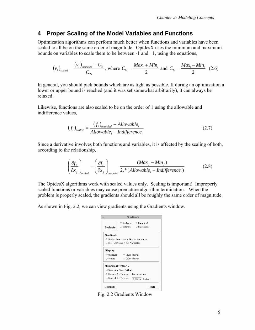
4 Proper Scaling of the Model Variables and Functions
Optimization algorithms can perform much better when functions and variables have been scaled to all be on the same order of magnitude. OptdesX uses the minimum and maximum bounds on variables to scale them to be between -1 and +1, using the equations,
i
iunscalediscaledi C
Cvv
2
1 , where
21ii
i
MinMaxC
and 2 2
i ii
Max MinC
(2.6)
In general, you should pick bounds which are as tight as possible. If during an optimization a lower or upper bound is reached (and it was set somewhat arbitrarily), it can always be relaxed. Likewise, functions are also scaled to be on the order of 1 using the allowable and indifference values,
ii
iunscalediscaledi ceIndifferenAllowable
Allowableff
(2.7)
Since a derivative involves both functions and variables, it is affected by the scaling of both, according to the relationship,
)(*.2
)(
ii
jj
unscaledj
i
scaledj
i
ceIndifferenAllowable
MinMax
x
f
x
f
(2.8)
The OptdesX algorithms work with scaled values only. Scaling is important! Improperly scaled functions or variables may cause premature algorithm termination. When the problem is properly scaled, the gradients should all be roughly the same order of magnitude. As shown in Fig. 2.2, we can view gradients using the Gradients window.
Fig. 2.2 Gradients Window
Chapter 2: Modeling Concepts
6
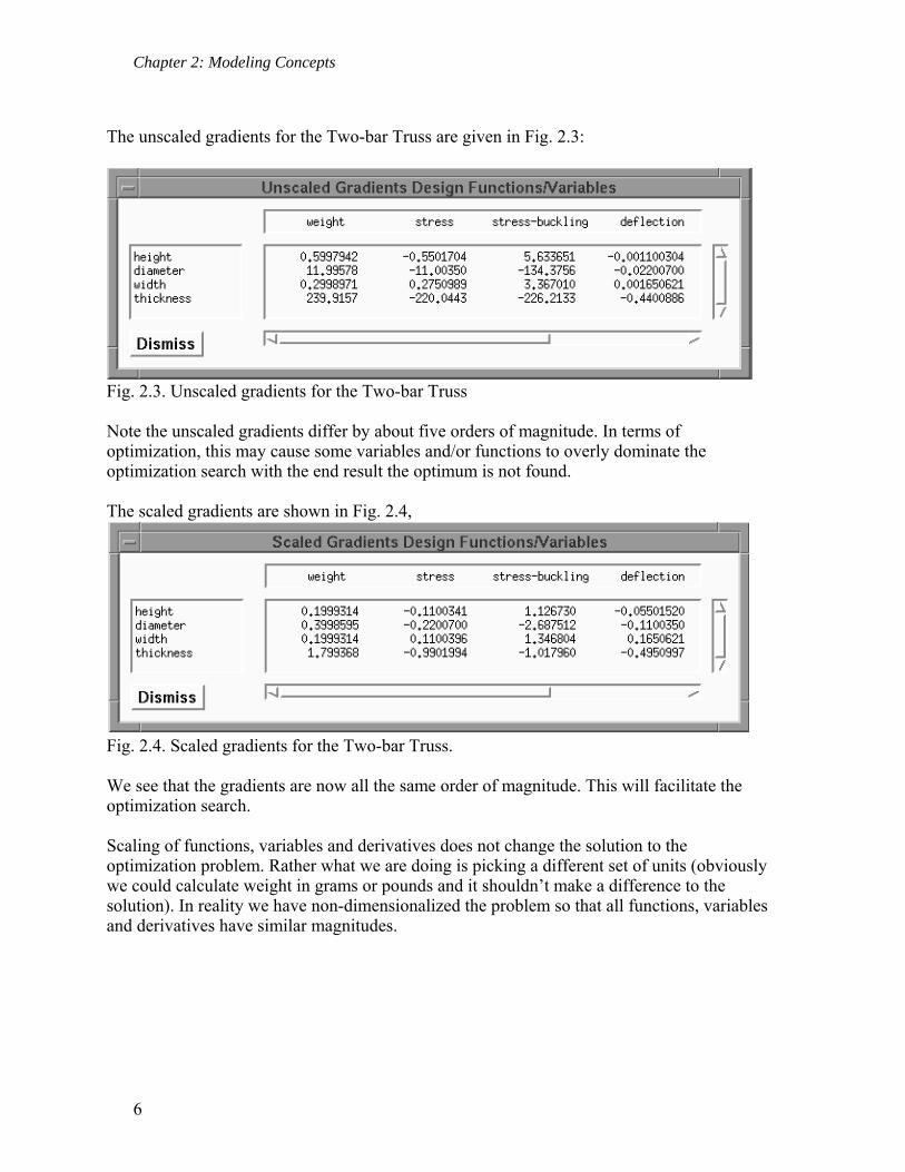
The unscaled gradients for the Two-bar Truss are given in Fig. 2.3:
Fig. 2.3. Unscaled gradients for the Two-bar Truss Note the unscaled gradients differ by about five orders of magnitude. In terms of optimization, this may cause some variables and/or functions to overly dominate the optimization search with the end result the optimum is not found. The scaled gradients are shown in Fig. 2.4,
Fig. 2.4. Scaled gradients for the Two-bar Truss. We see that the gradients are now all the same order of magnitude. This will facilitate the optimization search. Scaling of functions, variables and derivatives does not change the solution to the optimization problem. Rather what we are doing is picking a different set of units (obviously we could calculate weight in grams or pounds and it shouldn’t make a difference to the solution). In reality we have non-dimensionalized the problem so that all functions, variables and derivatives have similar magnitudes.
Chapter 2: Modeling Concepts
7
5 Formulating Objectives
5.1 Single Objective Problems
Most optimization problems, by convention, have one objective. This is at least partially because the mathematics of optimization were developed for single objective problems. Multiple objectives are treated briefly in this chapter and more extensively in Chap. 5. Often in optimization the selection of the objective will be obvious: we wish to minimize pressure drop or maximize heat transfer, etc. However, sometimes we end up with a surrogate objective because we can’t quantify or easily compute the real objective. For example, it is common in structures to minimize weight, with the assumption the minimum weight structure will also be the minimum cost structure. This may not always be true, however. (In particular, if minimum weight is achieved by having every member be a different size, the optimum could be very expensive!) Thus the designer should always keep in mind the assumptions and limitations associated with the objective of the optimization problem. Often in design problems there are other objectives or constraints for the problem which we can’t include. For example, aesthetics or comfort are objectives which are often difficult to quantify. For some products, it might also be difficult to estimate cost as a function of the design variables. These other objectives or constraints must be factored in at some point in the design process. The presence of these other considerations means that the optimization problem only partially captures the scope of the design problem. Thus the results of an optimization should be considered as one piece of a larger puzzle. Usually a designer will explore the design space and develop a spectrum of designs which can be considered as final decisions are made.
5.2 Special Objectives: Error Functions
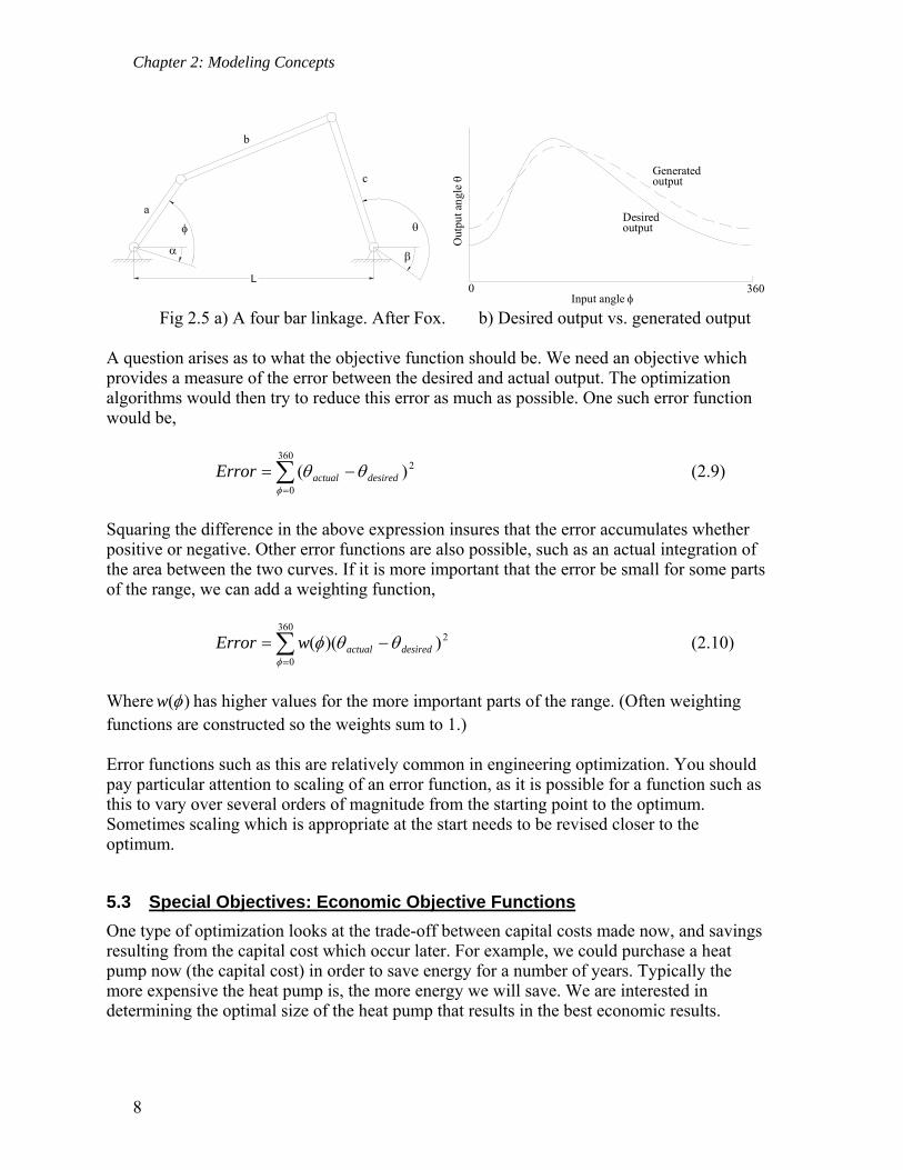
Consider the four bar linkage shown in the Fig. 2.5a below (from Optimization Methods for Engineering Design, R.L. Fox, Addison Wesley, 1971). We would like the linkage to follow a particular path as given by the solid in line in Fig. 2.5b. The actual output of a particular design is given by the dashed line. In this case we would like to design a linkage such that the generated output and the desired out put match as closely as possible.
Chapter 2: Modeling Concepts
8
Generated
Out
put a
ngle
Input angle
Desiredoutput
output
a
b
c
L
Fig 2.5 a) A four bar linkage. After Fox. b) Desired output vs. generated output
A question arises as to what the objective function should be. We need an objective which provides a measure of the error between the desired and actual output. The optimization algorithms would then try to reduce this error as much as possible. One such error function would be,
2360
0
)(
desiredactualError (2.9)
Squaring the difference in the above expression insures that the error accumulates whether positive or negative. Other error functions are also possible, such as an actual integration of the area between the two curves. If it is more important that the error be small for some parts of the range, we can add a weighting function,
2360
0
))((
desiredactualwError (2.10)
Where )(w has higher values for the more important parts of the range. (Often weighting functions are constructed so the weights sum to 1.) Error functions such as this are relatively common in engineering optimization. You should pay particular attention to scaling of an error function, as it is possible for a function such as this to vary over several orders of magnitude from the starting point to the optimum. Sometimes scaling which is appropriate at the start needs to be revised closer to the optimum.
5.3 Special Objectives: Economic Objective Functions
One type of optimization looks at the trade-off between capital costs made now, and savings resulting from the capital cost which occur later. For example, we could purchase a heat pump now (the capital cost) in order to save energy for a number of years. Typically the more expensive the heat pump is, the more energy we will save. We are interested in determining the optimal size of the heat pump that results in the best economic results.
Chapter 2: Modeling Concepts
9
To do this properly we must take into account the time value of money. The fact that money earns interest means that one dollar today is worth more than one dollar tomorrow. If the interest rate is 5%, compounded annually, $1.00 today is the same as $1.05 in one year. If expenses and/or savings are made at different times, we must convert them to the same time to make a proper comparison. This is the subject for engineering economics, so we will only briefly treat the subject here. One approach to examining the economics of projects is called net present value (NPV). For this approach, all economic transactions are converted to equivalent values in the present. In general, outflows (expenses) are considered negative; inflows (savings or income) are considered positive. There are two formulas which will be useful to us. The present value of one future payment or receipt, F, at period n with interest rate i is,
n
n
i
FP
)1( (2.11)
This equation allows us to convert any future value to the present. This might not be very convenient, however, if we have many future values to convert, particularly if we have a series of uniform payments. The present value of a series of uniform amounts, A, where the first payment is made at the end of the first period is given by,
n
n
ii
iAP
)1(
1)1(
(2.12)
5.3.1 Example: Net Present Value of Heat Pump
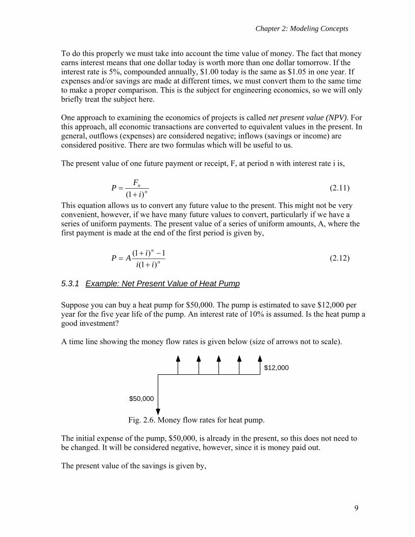
Suppose you can buy a heat pump for $50,000. The pump is estimated to save $12,000 per year for the five year life of the pump. An interest rate of 10% is assumed. Is the heat pump a good investment? A time line showing the money flow rates is given below (size of arrows not to scale).
$50,000
$12,000
Fig. 2.6. Money flow rates for heat pump.
The initial expense of the pump, $50,000, is already in the present, so this does not need to be changed. It will be considered negative, however, since it is money paid out. The present value of the savings is given by,
Chapter 2: Modeling Concepts
10
489,45$)1.01(1.0
1)1.01(000,12$
5
5
P (2.13)
4510$489,45$000,50$ NPV
Since the Net Present Value is negative, this is not a good investment. This result might be a little surprising, since without taking into account the time value of money, the total savings is 5*$12,000 = $60,000. However, at 10% interest, the value of the savings, when brought back to the present, does not equal the value of the $50,000 investment. This means we would be better off investing the $50,000 at 10% than using it to buy the heat pump. Note that (2.13) above assumes the first $12,000 of savings is realized at the end of the first period, as shown by the timeline for the example. When used in optimization, we would like to maximize net present value. In terms of the example, as we change the size of the heat pump (by changing, for example, the size of the heat exchangers and compressor), we change the initial cost and the annual savings. Question: How would the example change if the heat pump had some salvage value at the end of the five years?
6 Formulating Constraints
6.1 Inequality and Equality Constraints
Almost all engineering problems are constrained. Constraints can be either inequality constraints ib or ib ) or equality constraints ( ib ). The feasible region for inequality
constraints represents the entire area on the feasible side of the allowable value; for equality constraints, the feasible region is only where the constraint is equal to the allowable value itself. Because equality constraints are so restrictive, they should be avoided in optimization models whenever possible (an exception would be linear constraints, which are easily handled). If the constraint is simple, this can often be done by solving for the value of a variable explicitly. This eliminates a design variable and the equality constraint from the problem.
6.1.1 Example: Eliminating an Equality Constraint
Suppose we have the following equality constraint in our model, 2 2
1 2 10x x (2.14)
Chapter 2: Modeling Concepts
11
Where 1x and 2x are design variables. How would we include this constraint in our
optimization model? We have two choices. The choices are mathematically equivalent but one choice is much easier to optimize than the other. First choice: Keep 1x and 2x as design variables. Calculate the function,
2 2
1 2g x x (2.15)
Send this analysis function to the optimizer, and define the function as an equality constraint which is set equal to 10. Second choice: Solve for 1x explicitly in the analysis model,
21 210x x (2.16)
This eliminates 1x as a design variable (since its value is calculated, it cannot be adjusted
independently by the optimizer) and eliminates the equality constraint. The equality constraint is now implicitly embedded in the analysis model. Which choice is better for optimization? The second choice is a better way to go hands down: it eliminates a design variable and a highly restrictive equality constraint. The second choice results in a simpler optimization model. In one respect, however, the second choice is not as good: we can no longer explicitly put bounds on 1x like we could with the first choice. Now the value of 1x is set by (2.16); we can
only control the range of values indirectly by the upper and lower bounds set for 2x . (Also,
we note we are only taking the positive roots of 1x . We could modify this, however.)
6.2 Constraints Where the Allowable Value is a Function
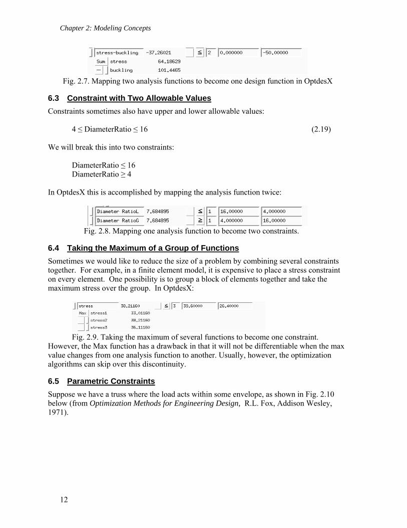
It is very common to have constraints of the form: Stress ≤ Buckling Stress (2.17) Most optimization routines, however, cannot handle a constraint that has a function for the right hand side. This is easily remedied by rewriting the function to be, Stress – Buckling Stress ≤ 0 (2.18) In OptdesX, this mapping can be done two ways: in your analysis routine you can create a function which computes stress minus buckling stress, or you can make the mapping directly in the OptdesX interface:
Chapter 2: Modeling Concepts
12
Fig. 2.7. Mapping two analysis functions to become one design function in OptdesX
6.3 Constraint with Two Allowable Values
Constraints sometimes also have upper and lower allowable values: 4 ≤ DiameterRatio ≤ 16 (2.19) We will break this into two constraints: DiameterRatio ≤ 16 DiameterRatio ≥ 4 In OptdesX this is accomplished by mapping the analysis function twice:
Fig. 2.8. Mapping one analysis function to become two constraints.
6.4 Taking the Maximum of a Group of Functions
Sometimes we would like to reduce the size of a problem by combining several constraints together. For example, in a finite element model, it is expensive to place a stress constraint on every element. One possibility is to group a block of elements together and take the maximum stress over the group. In OptdesX:
Fig. 2.9. Taking the maximum of several functions to become one constraint.
However, the Max function has a drawback in that it will not be differentiable when the max value changes from one analysis function to another. Usually, however, the optimization algorithms can skip over this discontinuity.
6.5 Parametric Constraints
Suppose we have a truss where the load acts within some envelope, as shown in Fig. 2.10 below (from Optimization Methods for Engineering Design, R.L. Fox, Addison Wesley, 1971).
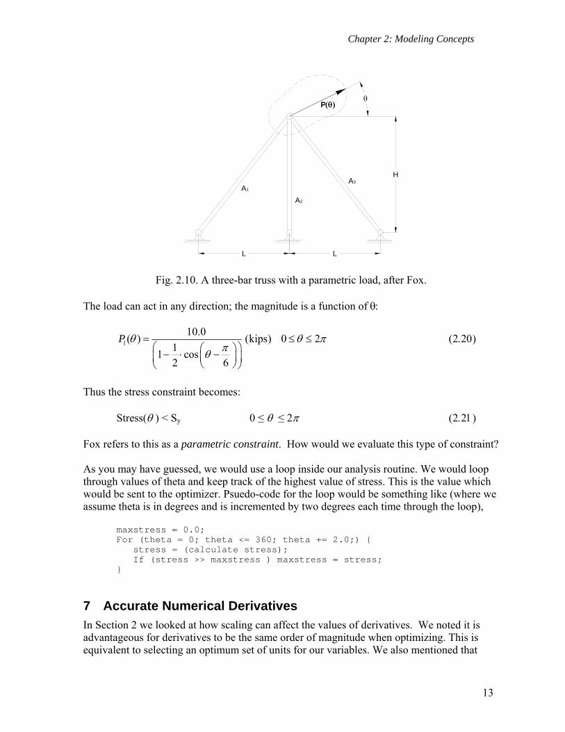
Chapter 2: Modeling Concepts
13
L
H
P
L
P
A1
A2
A3
Fig. 2.10. A three-bar truss with a parametric load, after Fox. The load can act in any direction; the magnitude is a function of
1
10.0( ) (kips) 0 2
11 cos
2 6
P
Thus the stress constraint becomes: Stress() < Sy 0 ≤ ≤ 2 Fox refers to this as a parametric constraint. How would we evaluate this type of constraint? As you may have guessed, we would use a loop inside our analysis routine. We would loop through values of theta and keep track of the highest value of stress. This is the value which would be sent to the optimizer. Psuedo-code for the loop would be something like (where we assume theta is in degrees and is incremented by two degrees each time through the loop), maxstress = 0.0; For (theta = 0; theta <= 360; theta += 2.0;) { stress = (calculate stress); If (stress >> maxstress ) maxstress = stress; }
7 Accurate Numerical Derivatives
In Section 2 we looked at how scaling can affect the values of derivatives. We noted it is advantageous for derivatives to be the same order of magnitude when optimizing. This is equivalent to selecting an optimum set of units for our variables. We also mentioned that
Chapter 2: Modeling Concepts
14
noise in the model can introduce error into derivatives. In this section we will look carefully at errors in numerical derivatives and learn how to reduce them. This is crucial if we expect a successful optimization.
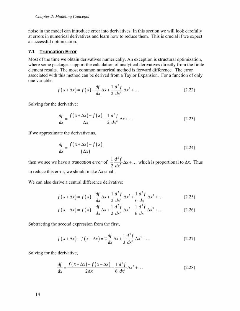
7.1 Truncation Error
Most of the time we obtain derivatives numerically. An exception is structural optimization, where some packages support the calculation of analytical derivatives directly from the finite element results. The most common numerical method is forward difference. The error associated with this method can be derived from a Taylor Expansion. For a function of only one variable:
2
22
1
2
df d ff x x f x x x
dx dx (2.22)
Solving for the derivative:
2
2
1
2
f x x f xdf d fx
dx x dx
(2.23)
If we approximate the derivative as,
f x x f xdf
dx x
(2.24)
then we see we have a truncation error of 2
2
1
2
d fx
dx which is proportional to x. Thus
to reduce this error, we should make x small. We can also derive a central difference derivative:
2 3
2 32 3
1 1
2 6
df d f d ff x x f x x x x
dx dx dx (2.25)
2 3
2 32 3
1 1
2 6
df d f d ff x x f x x x x
dx dx dx (2.26)
Subtracting the second expression from the first,
3
33
12
3
df d ff x x f x x x x
dx dx (2.27)
Solving for the derivative,
3
23
1
2 6
f x x f x xdf d fx
dx x dx
(2.28)
Chapter 2: Modeling Concepts
15
If we approximate the derivative as,
2
f x x f x xdf
dx x
(2.29)
then the truncation error is 3
23
1
6
d fx
dx , which is proportional to 2x .
Assuming x < 1.0, the central difference method should have less error than the forward difference method. For example, if x = 0.01, the truncation error for the central difference derivative should be proportional to 2(0.01) 0.0001 . If the error of the central difference method is better, why isn’t it the default? Because there is no free lunch! The central difference method requires two functions calls per derivative instead of one for the forward difference method. If we have 10 design variables, this means we have to call the analysis routine 20 times (twice for each variable) to get the derivatives instead of ten times. This can be prohibitively expensive.
7.2 Round-off Error
Besides truncation error, we also have round-off error. This is error associated with the number of significant figures in the function values. Returning to our expression for a forward difference derivative,
2
2
1
2
f x x f xdf d fx
dx x dx
(2.30)
2
2
2 1
2
f x x f xdf d fx
dx x x dx
(2.31)
where represents the error in the true function value caused by a lack of significant
figures. Recall that the true derivative is,
2
2
1
2
f x x f xdf d fx
dx x dx
(2.32)
but we are estimating it as,
2f x x f xdf
dx x x
(2.33)
where this last term is the round-off error. The total error is therefore,
Chapter 2: Modeling Concepts
16
2
2
2 1
2
d fx
x dx
(2.34)
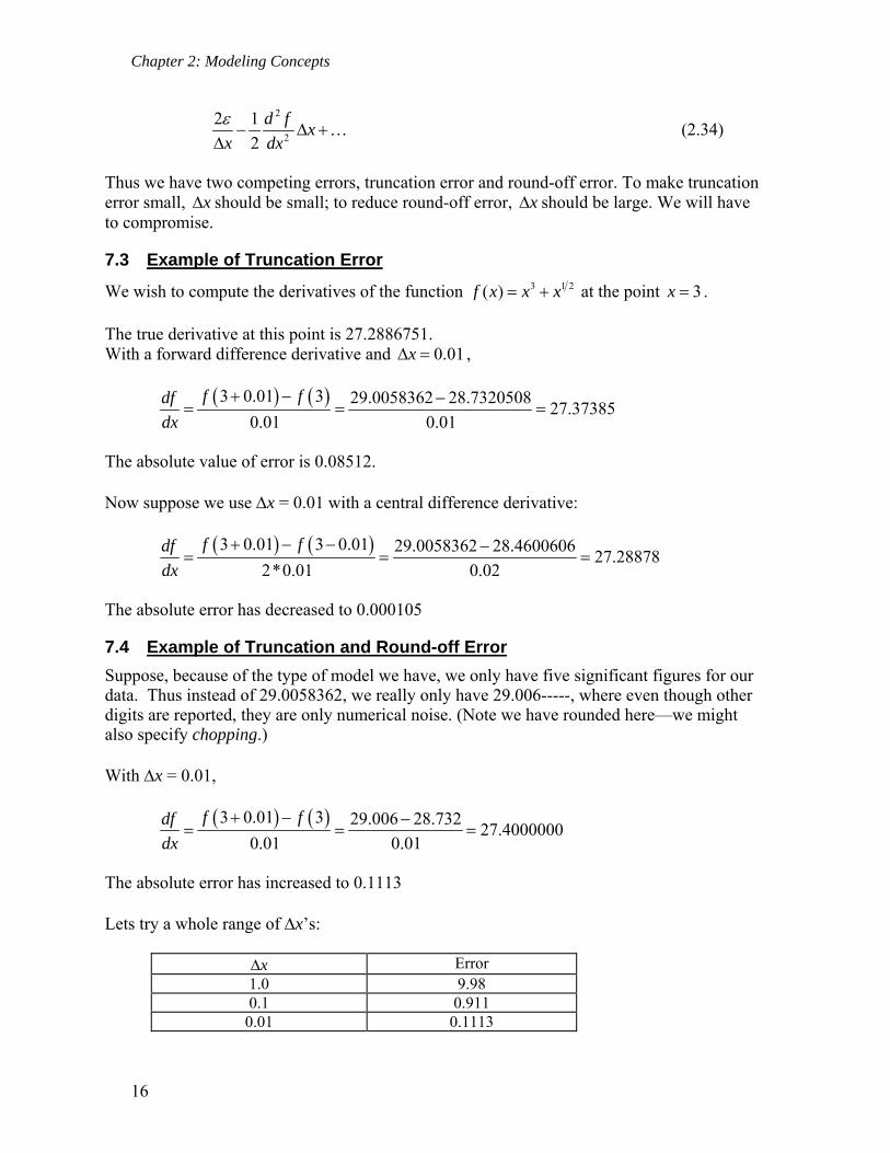
Thus we have two competing errors, truncation error and round-off error. To make truncation error small, x should be small; to reduce round-off error, x should be large. We will have to compromise.
7.3 Example of Truncation Error
We wish to compute the derivatives of the function 3 1 2( )f x x x at the point 3x . The true derivative at this point is 27.2886751. With a forward difference derivative and 0.01x ,
3 0.01 3 29.0058362 28.732050827.37385
0.01 0.01
f fdf
dx
The absolute value of error is 0.08512. Now suppose we use x = 0.01 with a central difference derivative:
3 0.01 3 0.01 29.0058362 28.460060627.28878
2*0.01 0.02
f fdf
dx
The absolute error has decreased to 0.000105
7.4 Example of Truncation and Round-off Error
Suppose, because of the type of model we have, we only have five significant figures for our data. Thus instead of 29.0058362, we really only have 29.006-----, where even though other digits are reported, they are only numerical noise. (Note we have rounded here—we might also specify chopping.) With x = 0.01,
3 0.01 3 29.006 28.732
27.40000000.01 0.01
f fdf
dx
The absolute error has increased to 0.1113 Lets try a whole range of x’s:
x Error 1.0 9.98 0.1 0.911
0.01 0.1113
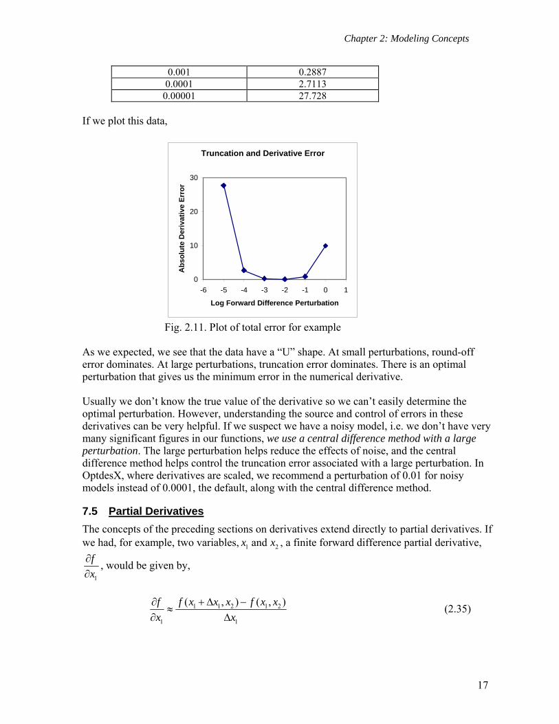
Chapter 2: Modeling Concepts
17
0.001 0.2887 0.0001 2.7113
0.00001 27.728 If we plot this data,
Truncation and Derivative Error
0
10
20
30
-6 -5 -4 -3 -2 -1 0 1
Log Forward Difference Perturbation
Ab
solu
te D
eriv
ativ
e E
rro
r
Fig. 2.11. Plot of total error for example
As we expected, we see that the data have a “U” shape. At small perturbations, round-off error dominates. At large perturbations, truncation error dominates. There is an optimal perturbation that gives us the minimum error in the numerical derivative. Usually we don’t know the true value of the derivative so we can’t easily determine the optimal perturbation. However, understanding the source and control of errors in these derivatives can be very helpful. If we suspect we have a noisy model, i.e. we don’t have very many significant figures in our functions, we use a central difference method with a large perturbation. The large perturbation helps reduce the effects of noise, and the central difference method helps control the truncation error associated with a large perturbation. In OptdesX, where derivatives are scaled, we recommend a perturbation of 0.01 for noisy models instead of 0.0001, the default, along with the central difference method.
7.5 Partial Derivatives
The concepts of the preceding sections on derivatives extend directly to partial derivatives. If we had, for example, two variables, 1 2andx x , a finite forward difference partial derivative,
1
f
x
, would be given by,
1 1 2 1 2
1 1
( , ) ( , )f x x x f x xf
x x
(2.35)
Chapter 2: Modeling Concepts
18
Note that only 1x is perturbed to evaluate the derivative. This variable would be set back to
its base value and 2x perturbed to find 2
f
x
.
In a similar manner, a central difference partial derivative for 1
f
x
would be given by,
1 1 2 1 1 2
1 1
( , ) ( , )
2
f x x x f x x xf
x x
(2.36)
8 Interpreting Graphics
This section may seem a disconnected subject—interpreting graphs of the design space. However graphs of the design space can tell us a lot about our model. If we can afford the computation, it can be very helpful to look at graphs of design space. OptdesX supports two basic types of plots: sensitivity plots (where functions are plotted with respect to one variable) and contour plots (where functions are plotted with respect to two variables). To create a sensitivity plot, one variable is changed at equal intervals, according to the number of points specified, and the analysis routine is called at each point. If ten points are used, the analysis routine is called ten times. The function values are stored in a file—this file is then graphed. To create a contour plot, two variables are changed at equal intervals (creating a mesh in the space) and the values stored in a file. If ten points are used for each variable, the analysis routine is called 100 times. Some points to remember:
•Use graphs to help you verify your model. Do the plots make sense? •Graphs can provide additional evidence that you have a global optimum. If the contours and constraint boundaries are smooth and relatively linear, then there are probably not a lot of local optima. Remember, though, you are usually only looking at a slice of design space. •When you generate a contour plot, remember that all variables except the two being changed are held constant at their current values. Thus if you wish to see what the design space looks like around the optimum, you must be at an optimum. •Graphs can often show why the algorithms may be having trouble, i.e. they can show that the design space is highly nonlinear, that the feasible region is disjoint, that functions are not smooth, etc. •Graphs are interpolated from an underlying mesh. Make sure the mesh is adequate. The mesh must be fine enough to capture the features of the space (see example in manual pg 10-9 to 10-10). Also, you need to make sure that the ranges for the variables, set in the
Chapter 2: Modeling Concepts
19
Explore window, are such that the designs are meaningful. In some cases, if the ranges are not appropriate, you may generate designs that are undefined, and values such as “Infinity” or “NaN” will be written into the Explore file. OptdesX cannot graph such a file and will give you an error message. •Optimal explore graphs show how the optimum changes as we change two analysis variables. (We cannot change two design variables—these are adjusted by the software to achieve an optimum.) These types of plots, where an optimization is performed at each mesh point, can be expensive. You must be very careful to set ranges so that an optimum can be found at each mesh point.
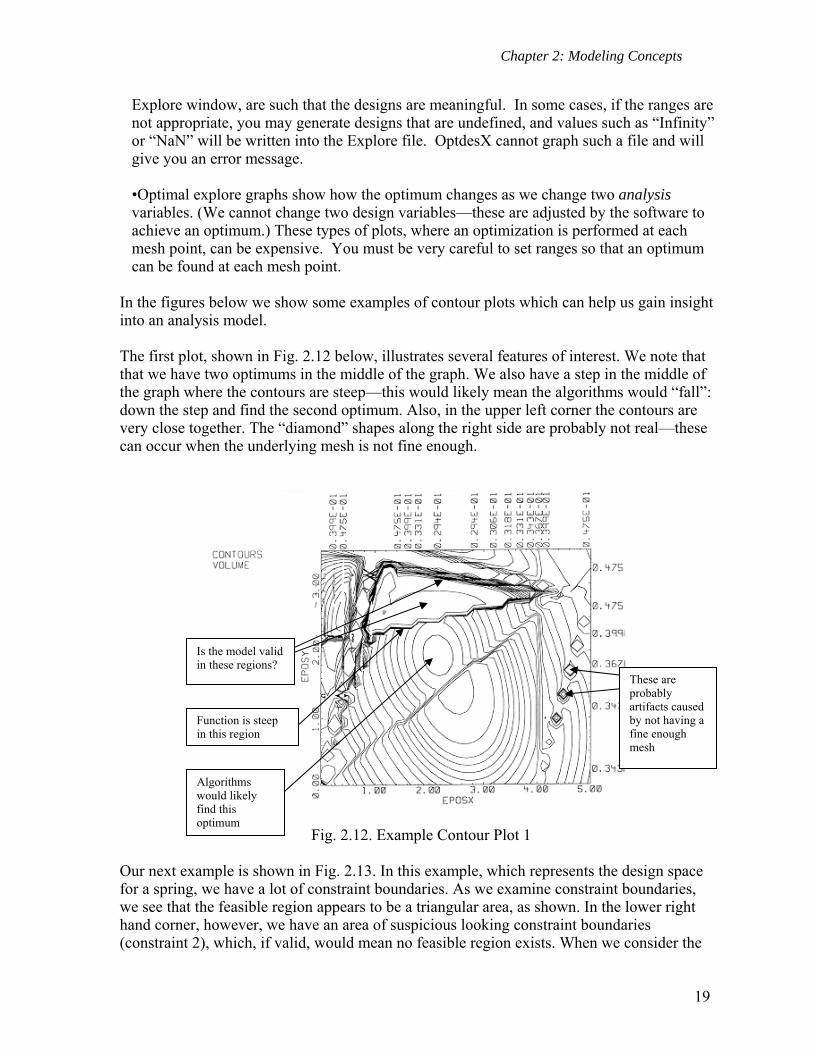
In the figures below we show some examples of contour plots which can help us gain insight into an analysis model. The first plot, shown in Fig. 2.12 below, illustrates several features of interest. We note that that we have two optimums in the middle of the graph. We also have a step in the middle of the graph where the contours are steep—this would likely mean the algorithms would “fall”: down the step and find the second optimum. Also, in the upper left corner the contours are very close together. The “diamond” shapes along the right side are probably not real—these can occur when the underlying mesh is not fine enough.
Fig. 2.12. Example Contour Plot 1
Our next example is shown in Fig. 2.13. In this example, which represents the design space for a spring, we have a lot of constraint boundaries. As we examine constraint boundaries, we see that the feasible region appears to be a triangular area, as shown. In the lower right hand corner, however, we have an area of suspicious looking constraint boundaries (constraint 2), which, if valid, would mean no feasible region exists. When we consider the
Function is steep in this region
These are probably artifacts caused by not having a fine enough mesh
Algorithms would likely find this optimum
Is the model valid in these regions?

Chapter 2: Modeling Concepts
20
values of variables in this area, however, we understand that this boundary is bogus. In this part of the plot, the wire diameter is greater than the coil diameter. Since this is impossible with a real spring, we know this boundary is bogus and can be ignored.
Fig. 2.13. Example Contour Plot 2
Our third and final example is given in Fig. 2.14. This is a sensitivity plot. Plots 2,3,4,5 look pretty reasonable. Plot 1, however, exhibits some noise. We would need to take this into account when numerical derivatives are computed. (Recall that we would want to use a central difference scheme with a larger perturbation.)
Fig. 2.14. Example Sensitivity Plot
This constraint is bogus
Feasible region is here
This plot shows the function is noisy.
Chapter 2: Modeling Concepts
21
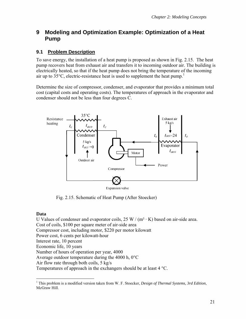
9 Modeling and Optimization Example: Optimization of a Heat Pump
9.1 Problem Description
To save energy, the installation of a heat pump is proposed as shown in Fig. 2.15. The heat pump recovers heat from exhaust air and transfers it to incoming outdoor air. The building is electrically heated, so that if the heat pump does not bring the temperature of the incoming air up to 35°C, electric-resistance heat is used to supplement the heat pump.1 Determine the size of compressor, condenser, and evaporator that provides a minimum total cost (capital costs and operating costs). The temperatures of approach in the evaporator and condenser should not be less than four degrees C.
Fig. 2.15. Schematic of Heat Pump (After Stoecker)
Data U Values of condenser and evaporator coils, 25 W / (m² · K) based on air-side area. Cost of coils, $100 per square meter of air-side area Compressor cost, including motor, $220 per motor kilowatt Power cost, 6 cents per kilowatt-hour Interest rate, 10 percent Economic life, 10 years Number of hours of operation per year, 4000 Average outdoor temperature during the 4000 h, 0°C Air flow rate through both coils, 5 kg/s Temperatures of approach in the exchangers should be at least 4 °C.
1 This problem is a modified version taken from W. F. Stoecker, Design of Thermal Systems, 3rd Edition, McGraw Hill.
Chapter 2: Modeling Concepts
22
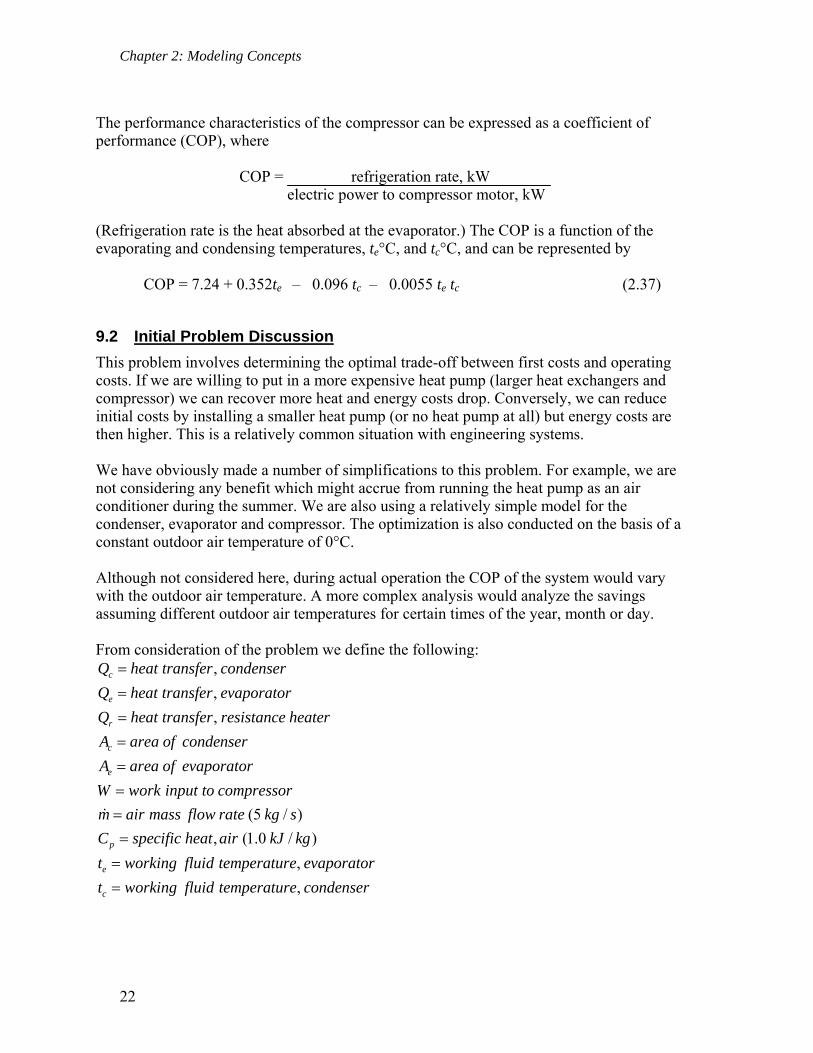
The performance characteristics of the compressor can be expressed as a coefficient of performance (COP), where
COP = refrigeration rate, kW electric power to compressor motor, kW
(Refrigeration rate is the heat absorbed at the evaporator.) The COP is a function of the evaporating and condensing temperatures, te°C, and tc°C, and can be represented by COP = 7.24 + 0.352te – 0.096 tc – 0.0055 te tc (2.37)
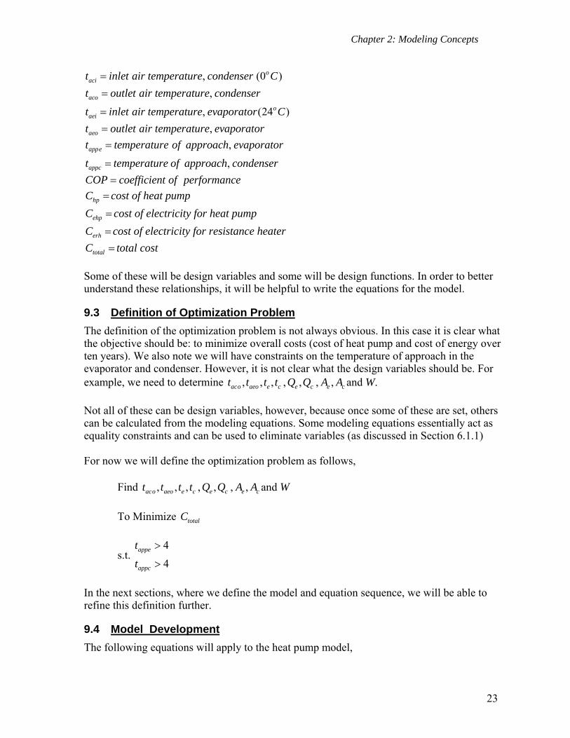
9.2 Initial Problem Discussion
This problem involves determining the optimal trade-off between first costs and operating costs. If we are willing to put in a more expensive heat pump (larger heat exchangers and compressor) we can recover more heat and energy costs drop. Conversely, we can reduce initial costs by installing a smaller heat pump (or no heat pump at all) but energy costs are then higher. This is a relatively common situation with engineering systems. We have obviously made a number of simplifications to this problem. For example, we are not considering any benefit which might accrue from running the heat pump as an air conditioner during the summer. We are also using a relatively simple model for the condenser, evaporator and compressor. The optimization is also conducted on the basis of a constant outdoor air temperature of 0°C. Although not considered here, during actual operation the COP of the system would vary with the outdoor air temperature. A more complex analysis would analyze the savings assuming different outdoor air temperatures for certain times of the year, month or day. From consideration of the problem we define the following:
,
,
,
(5 / )
, (1.0 / )
c
e
r
c
e
p
Q heat transfer condenser
Q heat transfer evaporator
Q heat transfer resistance heater
A area of condenser
A area of evaporator
W work input to compressor
m air mass flow rate kg s
C specific heat air kJ kg
,
,e
c
t working fluid temperature evaporator
t working fluid temperature condenser
Chapter 2: Modeling Concepts
23
, (0 )
,
, (24 )
oaci
aco
oaei
t inlet air temperature condenser C
t outlet air temperature condenser
t inlet air temperature evaporator C
,aeot outlet air temperature evaporator
,
,
appe
appc
t temperature of approach evaporator
t temperature of approach condenser
COP coefficient of performance
hpC cost of heat pump
ehpC cost of electricity for heat pump
erhC cost of electricity for resistance heater
totalC total cost
Some of these will be design variables and some will be design functions. In order to better understand these relationships, it will be helpful to write the equations for the model.
9.3 Definition of Optimization Problem
The definition of the optimization problem is not always obvious. In this case it is clear what the objective should be: to minimize overall costs (cost of heat pump and cost of energy over ten years). We also note we will have constraints on the temperature of approach in the evaporator and condenser. However, it is not clear what the design variables should be. For example, we need to determine , , ,aco aeo e ct t t t , ,e cQ Q , ,e cA A and W.
Not all of these can be design variables, however, because once some of these are set, others can be calculated from the modeling equations. Some modeling equations essentially act as equality constraints and can be used to eliminate variables (as discussed in Section 6.1.1) For now we will define the optimization problem as follows, Find , , ,aco aeo e ct t t t , ,e cQ Q , ,e cA A and W
To Minimize totalC
s.t. 4
4
appe
appc
t
t
In the next sections, where we define the model and equation sequence, we will be able to refine this definition further.
9.4 Model Development
The following equations will apply to the heat pump model,
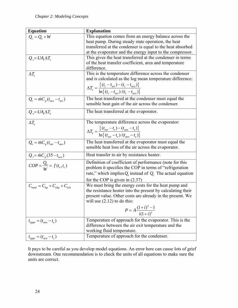
Chapter 2: Modeling Concepts
24
Equation Explanation
c eQ Q W This equation comes from an energy balance across the heat pump. During steady state operation, the heat transferred at the condenser is equal to the heat absorbed at the evaporator and the energy input to the compressor.
c c cQ UA T This gives the heat transferred at the condenser in terms of the heat transfer coefficient, area and temperature difference.
cT This is the temperature difference across the condenser and is calculated as the log mean temperature difference:
( ) ( )
ln ( ) /( )c aci c aco
cc aci c aco
t t t tT
t t t t
( )c p aco aciQ mC t t
The heat transferred at the condenser must equal the sensible heat gain of the air across the condenser.
e e eQ UA T The heat transferred at the evaporator.
eT The temperature difference across the evaporator: ( ) ( )
ln ( ) /( )aei e aeo e
eaei e aeo e
t t t tT
t t t t
( )e p aei aeoQ mC t t
The heat transferred at the evaporator must equal the sensible heat loss of the air across the evaporator.
(35 )r p acoQ mC t Heat transfer to air by resistance heater.
),( cee ttf
W
QCOP
Definition of coefficient of performance (note for this problem it specifies the COP in terms of “refrigeration rate,” which implies eQ instead of cQ The actual equation
for the COP is given in (2.37)
total hp ehp erhC C C C
We must bring the energy costs for the heat pump and the resistance heater into the present by calculating their present value. Other costs are already in the present. We will use (2.12) to do this:
n
n
ii
iAP
)1(
1)1(
( )appe aeo et t t Temperature of approach for the evaporator. This is the difference between the air exit temperature and the working fluid temperature.
( )appc aco ct t t Temperature of approach for the condenser.
It pays to be careful as you develop model equations. An error here can cause lots of grief downstream. One recommendation is to check the units of all equations to make sure the units are correct.
Chapter 2: Modeling Concepts
25
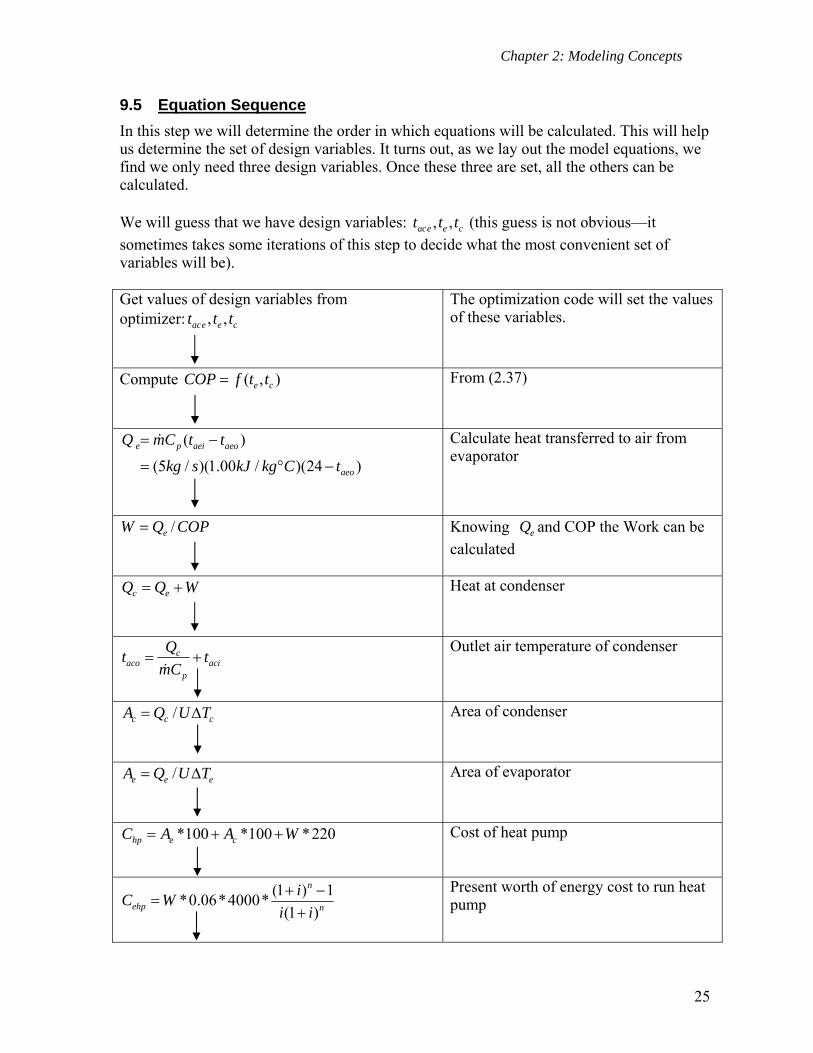
9.5 Equation Sequence
In this step we will determine the order in which equations will be calculated. This will help us determine the set of design variables. It turns out, as we lay out the model equations, we find we only need three design variables. Once these three are set, all the others can be calculated. We will guess that we have design variables: , ,ace e ct t t (this guess is not obvious—it
sometimes takes some iterations of this step to decide what the most convenient set of variables will be). Get values of design variables from optimizer: , ,ace e ct t t
The optimization code will set the values of these variables.
Compute ),( ce ttfCOP
From (2.37)
( )
(5 / )(1.00 / )(24 )
e p aei aeo
aeo
Q mC t t
kg s kJ kg C t
Calculate heat transferred to air from evaporator
COPQW e /
Knowing eQ and COP the Work can be
calculated
WQQ ec
Heat at condenser
caco aci
p
Qt t
mC
Outlet air temperature of condenser
/c c cA Q U T
Area of condenser
/e e eA Q U T
Area of evaporator
*100 *100 *220hp e cC A A W Cost of heat pump
(1 ) 1*0.06*4000*
(1 )
n
ehp n
iC W
i i
Present worth of energy cost to run heat pump
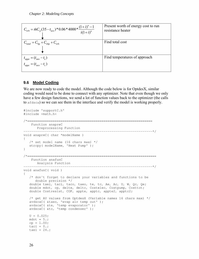
Chapter 2: Modeling Concepts
26
(1 ) 1(35 )*0.06*4000*
(1 )
n
erh p aco n
iC mC t
i i
Present worth of energy cost to run resistance heater
total hp ehp erhC C C C
Find total cost
( )appe aeo et t t
( )appc aco ct t t
Find temperatures of approach
9.6 Model Coding
We are now ready to code the model. Although the code below is for OptdesX, similar coding would need to be done to connect with any optimizer. Note that even though we only have a few design functions, we send a lot of function values back to the optimizer (the calls to afdsca) so we can see them in the interface and verify the model is working properly. #include "supportC.h" #include <math.h> /*================================================================ Function anapreC Preprocessing Function ------------------------------------------------------------------*/ void anapreC( char *modelName ) { /* set model name (16 chars max) */ strcpy( modelName, "Heat Pump" ); } /*================================================================== Function anafunC Analysis Function ------------------------------------------------------------------*/ void anafunC( void ) { /* don't forget to declare your variables and functions to be double precision */ double taei, taci, taco, taeo, te, tc, Ae, Ac, U, W, Qc, Qe; double mdot, cp, delte, deltc, Costelec, Costpump, Costtot; double Costresist, COP, appte, apptc, appte2, apptc2; /* get AV values from OptdesX (Variable names 16 chars max) */ avdscaC( &taeo, "evap air temp out" ); avdscaC( &te, "temp evaporator" ); avdscaC( &tc, "temp condenser" ); U = 0.025; mdot = 5.; cp = 1.00; taci = 0.; taei = 24.;
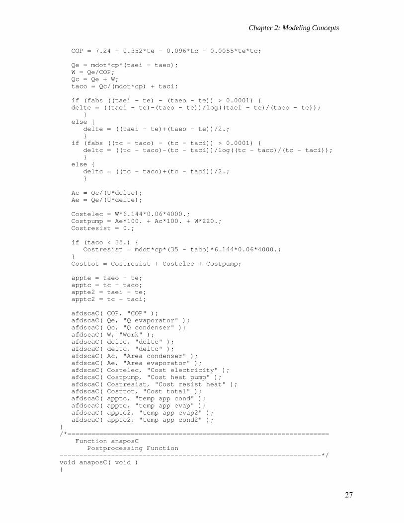
Chapter 2: Modeling Concepts
27
COP = 7.24 + 0.352*te - 0.096*tc - 0.0055*te*tc; Qe = mdot*cp*(taei - taeo); W = Qe/COP; Qc = Qe + W; taco = Qc/(mdot*cp) + taci; if (fabs ((taei - te) - (taeo - te)) > 0.0001) { delte = ((taei - te)-(taeo - te))/log((taei - te)/(taeo - te)); } else { delte = ((taei - te)+(taeo - te))/2.; } if (fabs ((tc - taco) - (tc - taci)) > 0.0001) { deltc = ((tc - taco)-(tc - taci))/log((tc - taco)/(tc - taci)); } else { deltc = ((tc - taco)+(tc - taci))/2.; } Ac = Qc/(U*deltc); Ae = Qe/(U*delte); Costelec = W*6.144*0.06*4000.; Costpump = Ae*100. + Ac*100. + W*220.; Costresist = 0.; if (taco < 35.) { Costresist = mdot*cp*(35 - taco)*6.144*0.06*4000.; } Costtot = Costresist + Costelec + Costpump; appte = taeo - te; apptc = tc - taco; appte2 = taei - te; apptc2 = tc - taci; afdscaC( COP, "COP" ); afdscaC( Qe, "Q evaporator" ); afdscaC( Qc, "Q condenser" ); afdscaC( W, "Work" ); afdscaC( delte, "delte" ); afdscaC( deltc, "deltc" ); afdscaC( Ac, "Area condenser" ); afdscaC( Ae, "Area evaporator" ); afdscaC( Costelec, "Cost electricity" ); afdscaC( Costpump, "Cost heat pump" ); afdscaC( Costresist, "Cost resist heat" ); afdscaC( Costtot, "Cost total" ); afdscaC( apptc, "temp app cond" ); afdscaC( appte, "temp app evap" ); afdscaC( appte2, "temp app evap2" ); afdscaC( apptc2, "temp app cond2" ); } /*================================================================== Function anaposC Postprocessing Function ------------------------------------------------------------------*/ void anaposC( void ) {
Chapter 2: Modeling Concepts
28
}
9.7 Linking and Verifying the Model
After we have coded and debugged the model, we link it to the optimizer and begin verification. (In some situations we might be able to verify the model before we link to the optimizer. In such a case we would be able to execute the model separately.) Verification involves checking the model at various points to make sure it is working properly. The values of the design variables are changed manually, and the compute functions button is pushed (causing OptdesX to call the model) to look at the corresponding function values. In this case, I spent over two hours debugging the model. Initially I noticed that no matter what the starting design was, the cost would evaluate to be higher for small perturbations of the design variable, aeot , regardless of whether I perturbed it smaller or larger. The problem was
finally traced down to the fact I was using “abs” for absolute value instead of “fabs” to get the absolute value of a real expression. This was causing erratic results in the model (“abs” is used to get the absolute value of integer expressions). I also discovered I had accidentally switched appet with appct . I did some “brute force” debugging to find these errors: I put in
several printf statements and printed out lots of values until I could track them down.
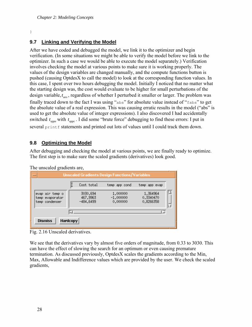
9.8 Optimizing the Model
After debugging and checking the model at various points, we are finally ready to optimize. The first step is to make sure the scaled gradients (derivatives) look good. The unscaled gradients are,
Fig. 2.16 Unscaled derivatives. We see that the derivatives vary by almost five orders of magnitude, from 0.33 to 3030. This can have the effect of slowing the search for an optimum or even causing premature termination. As discussed previously, OptdesX scales the gradients according to the Min, Max, Allowable and Indifference values which are provided by the user. We check the scaled gradients,
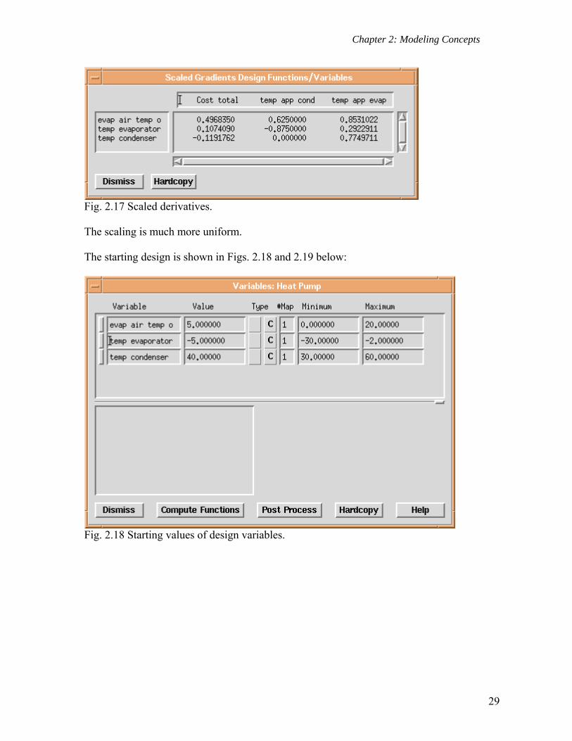
Chapter 2: Modeling Concepts
29
Fig. 2.17 Scaled derivatives. The scaling is much more uniform. The starting design is shown in Figs. 2.18 and 2.19 below:
Fig. 2.18 Starting values of design variables.
Chapter 2: Modeling Concepts
30
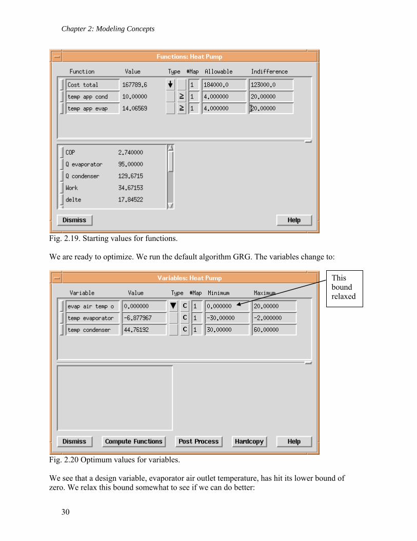
Fig. 2.19. Starting values for functions. We are ready to optimize. We run the default algorithm GRG. The variables change to:
Fig. 2.20 Optimum values for variables. We see that a design variable, evaporator air outlet temperature, has hit its lower bound of zero. We relax this bound somewhat to see if we can do better:
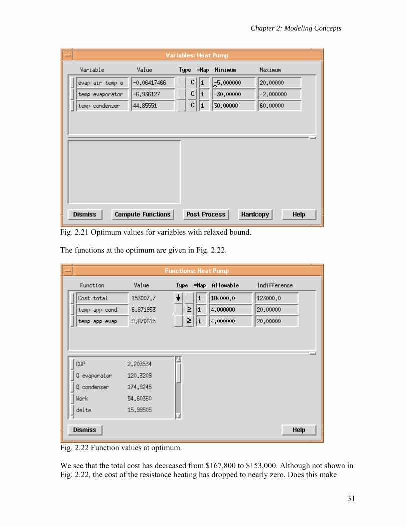
This bound relaxed
Chapter 2: Modeling Concepts
31
Fig. 2.21 Optimum values for variables with relaxed bound. The functions at the optimum are given in Fig. 2.22.
Fig. 2.22 Function values at optimum. We see that the total cost has decreased from $167,800 to $153,000. Although not shown in Fig. 2.22, the cost of the resistance heating has dropped to nearly zero. Does this make
Chapter 2: Modeling Concepts
32
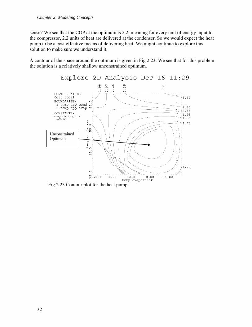
sense? We see that the COP at the optimum is 2.2, meaning for every unit of energy input to the compressor, 2.2 units of heat are delivered at the condenser. So we would expect the heat pump to be a cost effective means of delivering heat. We might continue to explore this solution to make sure we understand it. A contour of the space around the optimum is given in Fig 2.23. We see that for this problem the solution is a relatively shallow unconstrained optimum.
Fig 2.23 Contour plot for the heat pump.
Unconstrained Optimum