
05_Flows Modeling in Automotive
152
Projekt współfinansowany ze środków Unii Europejskiej w ramach Europejskiego Funduszu Społecznego ROZWÓJ POTENCJAŁU I OFERTY DYDAKTYCZNEJ POLITECHNIKI WROCŁAWSKIEJ Wrocław University of Technology Automotive Engineering Marcin Tkaczyk FLOWS MODELING IN AUTOMOTIVE ENGINEERING Wrocław 2011
Transcript of 05_Flows Modeling in Automotive
Projekt współfinansowany ze środków Unii Europejskiej w ramach Europejskiego Funduszu Społecznego
ROZWÓJ POTENCJAŁU I OFERTY DYDAKTYCZNEJ POLITECHNIKI WROCŁAWSKIEJ
Wrocław University of Technology
Automotive Engineering
Marcin Tkaczyk
FLOWS MODELING IN
AUTOMOTIVE ENGINEERING
Wrocław 2011
Wrocław University of Technology
Automotive Engineering
Marcin Tkaczyk
FLOWS MODELING IN
AUTOMOTIVE ENGINEERING Developing Engine Technology
Wrocław 2011
Copyright © by Wrocław University of Technology
Wrocław 2011
Reviewer: Jan Kulczyk
ISBN 978-83-62098-08-8
Published by PRINTPAP Łódź, www.printpap.pl

3
Table of contents
Introduction ................................................................................................................................ 5
1. Basis .................................................................................................................................... 5
1.1. Continuity and Momentum Equations ......................................................................... 5
1.2. Introduction for real flows ........................................................................................... 7
1.3. Choosing a Turbulence Model .................................................................................... 8
1.3.1. Transport Equation for the Spalart-Allmaras Model ............................................ 8
1.3.2. The Standard, RNG, and Realizable k- Models ............................................... 9
1.3.3. The Standard k- Model ..................................................................................... 9
1.3.4. Transport Equations for the Standard k- Model ................................................ 9
1.3.5. The RNG k- Model .......................................................................................... 11
1.3.6. The Realizable k- Model ................................................................................ 14
1.3.7. The Standard and SST k- Models ................................................................... 18
1.3.8. The Standard k- Model ................................................................................... 19
1.3.9. The Reynolds Stress Transport Equations ......................................................... 25
1.4. Solution Strategies for Turbulent Flow Simulations ................................................. 25
1.5. Mesh Generation ........................................................................................................ 26
1.6. Accuracy .................................................................................................................... 26
1.7. Convergence .............................................................................................................. 26
2. Aerodynamice ................................................................................................................... 28
3. Inlet and outlet in combustion engines ............................................................................. 37
4. MOVING/DEFORMING MESH ..................................................................................... 51
4.1. Conservation Equations ............................................................................................. 51
4.2. Defining Dynamic Mesh Events ................................................................................ 52
4.2.1. Procedure for Defining Events ........................................................................... 52
4.3. Using the In-Cylinder Model ..................................................................................... 58
4.3.1. Overview ............................................................................................................ 58
4.3.2. Defining Starting Position Mesh for the In-Cylinder Model ............................. 62
4.3.3. Defining Motion/Geometry Attributes of Mesh Zones ...................................... 63
4.3.4. Defining Valve Opening and Closure ................................................................ 69
4.3.5. Defining Events for In-Cylinder Applications ................................................... 69
5. Injection ............................................................................................................................ 70
5.1. Point Properties for Single Injections ........................................................................ 71
5.2. Point Properties for Group Injections ........................................................................ 71
5.3. Point Properties for Cone Injections .......................................................................... 75
5.4. Point Properties for Surface Injections ...................................................................... 77
6. Modeling Engine Ignition ................................................................................................. 79
6.1. Autoignition Models .................................................................................................. 79
6.1.1. Overview ............................................................................................................ 79
6.1.2. Model Limitations .............................................................................................. 79
6.2. Ignition Model Theory ............................................................................................... 80
6.3. Transport of Ignition Species .................................................................................... 80
6.4. Knock Modeling ........................................................................................................ 80
6.5. Ignition Delay Modeling ........................................................................................... 82
6.6. Modeling of the Source Term .................................................................................... 82
6.7. Correlations ............................................................................................................... 82
6.8. Using the Autoignition Models ................................................................................. 83
7. Modeling Species Transport and Finite-Rate Chemistry .................................................. 86
7.1. Theory ........................................................................................................................ 86
7.2. Overview of User Inputs for Modeling Species Transport and Reactions ................ 967.2.1. Enabling Species Transport and Reactions and Choosing the Mixture Material
987.2.2. Defining Properties for the Mixture and Its Constituent Species ..................... 1007.2.3. Defining Boundary Conditions for Species ..................................................... 113
7.3. Theory ...................................................................................................................... 1147.4. Species Transport Without Reactions ...................................................................... 1177.5. Modeling Non-Premixed Combustion ..................................................................... 118
7.5.1. Description of the Equilibrium Mixture Fraction/ PDF Model ........................ 1187.5.2. Benefits and Limitations of the Non-Premixed Approach ............................... 1187.5.3. Details of the Non-Premixed Approach ........................................................... 1197.5.4. Restrictions and Special Cases for the Non-Premixed Model ......................... 1377.5.5. Modeling Approaches for Non-Premixed Equilibrium Chemistry .................. 1417.5.5.1. Single-Mixture-Fraction Approach .............................................................. 141
7.6. Modeling Liquid Fuel Combustion Using the Non-Premixed Model .................... 1487.6.1. Adding New Species to the prePDF Database ................................................. 148
4

Introduction The aim of this course book is to present the theoretical fundamentals of numerical modeling issues accomplished within „Flows Modeling in Automotive Engineering” course.
- First chapter introduces fundamentals of modeling basing on mass conservation law, energy conservation law, principle of conservation of momentum supplemented with a turbulence models,
The course book follows the course chronology, therefore it was divided into five chapters of which:
- Second chapter describes the possibilities of modeling issues related with vehicle aerodynamics
- Third chapter describes modeling of an intake and exhaust systems of a piston combustion engines,
- Fourth chapter introduces fundamentals of modeling with usage of dynamic mesh, which are indispensable in terms of combustion process modeling within an piston combustion engine,
- Fifth chapter presents the theoretical deliberation of fuel injection into the cylinders of piston combustion engine,
- Sixth chapter describes the numerical modeling of an engine ignition system, - Seventh chapter describes numerical models of combustion process within the piston
combustion engine.
1. Basis [13] Following chapters describes the fundamentals of finite volume method on which the software used in „Flows Modeling in Automotive Engineering” is based.
1.1. Continuity and Momentum Equations
For all flows, FLUENT solves conservation equations for mass and momentum. For flows involving heat transfer or compressibility, an additional equation for energy conservation is solved. For flows involving species mixing or reactions, a species conservation equation is solved or, if the non-premixed combustion model is used, conservation equations for the mixture fraction and its variance are solved. Additional transport equations are also solved when the flow is turbulent.
In this section, the conservation equations for laminar flow (in an inertial (non-accelerating) reference frame) are presented. The conservation equations relevant to heat transfer, turbulence modeling, and species transport will be discussed in the chapters where those models are described.
The Mass Conservation Equation
The equation for conservation of mass, or continuity equation, can be written as follows:
(1.1)
5

Equation (1. 1) is the general form of the mass conservation equation and is valid for incompressible as well as compressible flows. The source S m
For 2D axisymmetric geometries, the continuity equation is given by
is the mass added to the continuous phase from the dispersed second phase (e.g., due to vaporization of liquid droplets) and any user-defined sources.
(1. 2)
where x is the axial coordinate, r is the radial coordinate, v x is the axial velocity, and v r
Momentum Conservation Equations
is the radial velocity.
Conservation of momentum in an inertial (non-accelerating) reference frame is described by [4]
(1. 3)
where p is the static pressure, is the stress tensor (described below), and and are the gravitational body force and external body forces (e.g., that arise from interaction with the dispersed phase), respectively. also contains other model-dependent source terms such as porous-media and user-defined sources.
The stress tensor is given by
(1. 4)
where is the molecular viscosity, I is the unit tensor, and the second term on the right hand side is the effect of volume dilation.
6
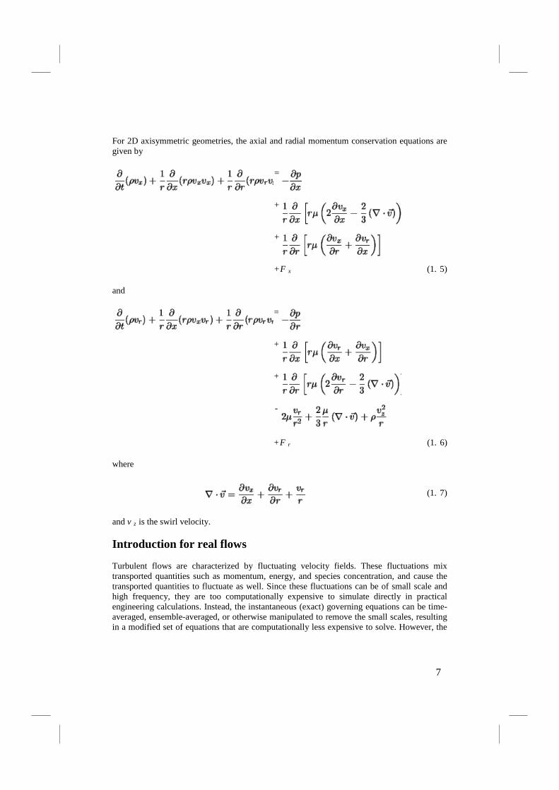
For 2D axisymmetric geometries, the axial and radial momentum conservation equations are given by
=
+
+
+ F (1. 5) x and
=
+
+
-
+ F (1. 6) r where
(1. 7)
and v z
is the swirl velocity.
Introduction for real flows
Turbulent flows are characterized by fluctuating velocity fields. These fluctuations mix transported quantities such as momentum, energy, and species concentration, and cause the transported quantities to fluctuate as well. Since these fluctuations can be of small scale and high frequency, they are too computationally expensive to simulate directly in practical engineering calculations. Instead, the instantaneous (exact) governing equations can be time-averaged, ensemble-averaged, or otherwise manipulated to remove the small scales, resulting in a modified set of equations that are computationally less expensive to solve. However, the
7

modified equations contain additional unknown variables, and turbulence models are needed to determine these variables in terms of known quantities.
FLUENT provides the following choices of turbulence models:
• Spalart-Allmaras model • k- models
o Standard k- model o Renormalization-group (RNG) k- model o Realizable k- model
• k- models o Standard k- model o Shear-stress transport (SST) k- model
• Reynolds stress model (RSM) • Large eddy simulation (LES) model
1.2. Choosing a Turbulence Model
It is an unfortunate fact that no single turbulence model is universally accepted as being superior for all classes of problems. The choice of turbulence model will depend on considerations such as the physics encompassed in the flow, the established practice for a specific class of problem, the level of accuracy required, the available computational resources, and the amount of time available for the simulation. To make the most appropriate choice of model for your application, you need to understand the capabilities and limitations of the various options.
The choice of turbulence model:
• Spalart-Allmaras Model • The Standard, RNG, and Realizable k- Models • The Standard k- Model • The RNG k- Model • The Standard and SST k- Models • The Reynolds Stress
1.2.1. Transport Equation for the Spalart-Allmaras Model
The transported variable in the Spalart-Allmaras model, , is identical to the turbulent kinematic viscosity except in the near-wall (viscous-affected) region. The transport equation for is
8
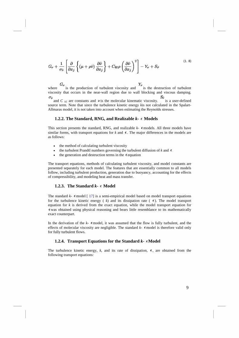
(1. 8)
where is the production of turbulent viscosity and is the destruction of turbulent viscosity that occurs in the near-wall region due to wall blocking and viscous damping.
and C b2 are constants and is the molecular kinematic viscosity. is a user-defined source term. Note that since the turbulence kinetic energy kis not calculated in the Spalart-Allmaras model, it is not taken into account when estimating the Reynolds stresses.
1.2.2. The Standard, RNG, and Realizable k- Models
This section presents the standard, RNG, and realizable k- models. All three models have similar forms, with transport equations for k and . The major differences in the models are as follows:
• the method of calculating turbulent viscosity • the turbulent Prandtl numbers governing the turbulent diffusion of k and • the generation and destruction terms in the equation
The transport equations, methods of calculating turbulent viscosity, and model constants are presented separately for each model. The features that are essentially common to all models follow, including turbulent production, generation due to buoyancy, accounting for the effects of compressibility, and modeling heat and mass transfer.
1.2.3. The Standard k- Model
The standard k- model [ 17] is a semi-empirical model based on model transport equations for the turbulence kinetic energy ( k) and its dissipation rate ( ). The model transport equation for k is derived from the exact equation, while the model transport equation for
was obtained using physical reasoning and bears little resemblance to its mathematically exact counterpart.
In the derivation of the k- model, it was assumed that the flow is fully turbulent, and the effects of molecular viscosity are negligible. The standard k- model is therefore valid only for fully turbulent flows.
1.2.4. Transport Equations for the Standard k- Model
The turbulence kinetic energy, k, and its rate of dissipation,
, are obtained from the following transport equations:
9
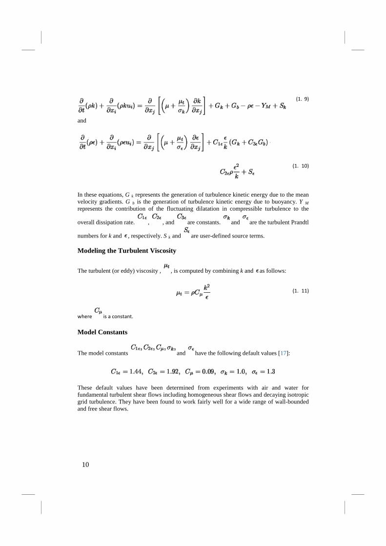
(1. 9)
and
(1. 10)
In these equations, G k represents the generation of turbulence kinetic energy due to the mean velocity gradients. G b is the generation of turbulence kinetic energy due to buoyancy. Y M represents the contribution of the fluctuating dilatation in compressible turbulence to the
overall dissipation rate. , , and are constants. and are the turbulent Prandtl
numbers for k and , respectively. S k and are user-defined source terms.
Modeling the Turbulent Viscosity
The turbulent (or eddy) viscosity ,
, is computed by combining k and as follows:
(1. 11)
where is a constant.
Model Constants
The model constants
and have the following default values [17]:
These default values have been determined from experiments with air and water for fundamental turbulent shear flows including homogeneous shear flows and decaying isotropic grid turbulence. They have been found to work fairly well for a wide range of wall-bounded and free shear flows.
10
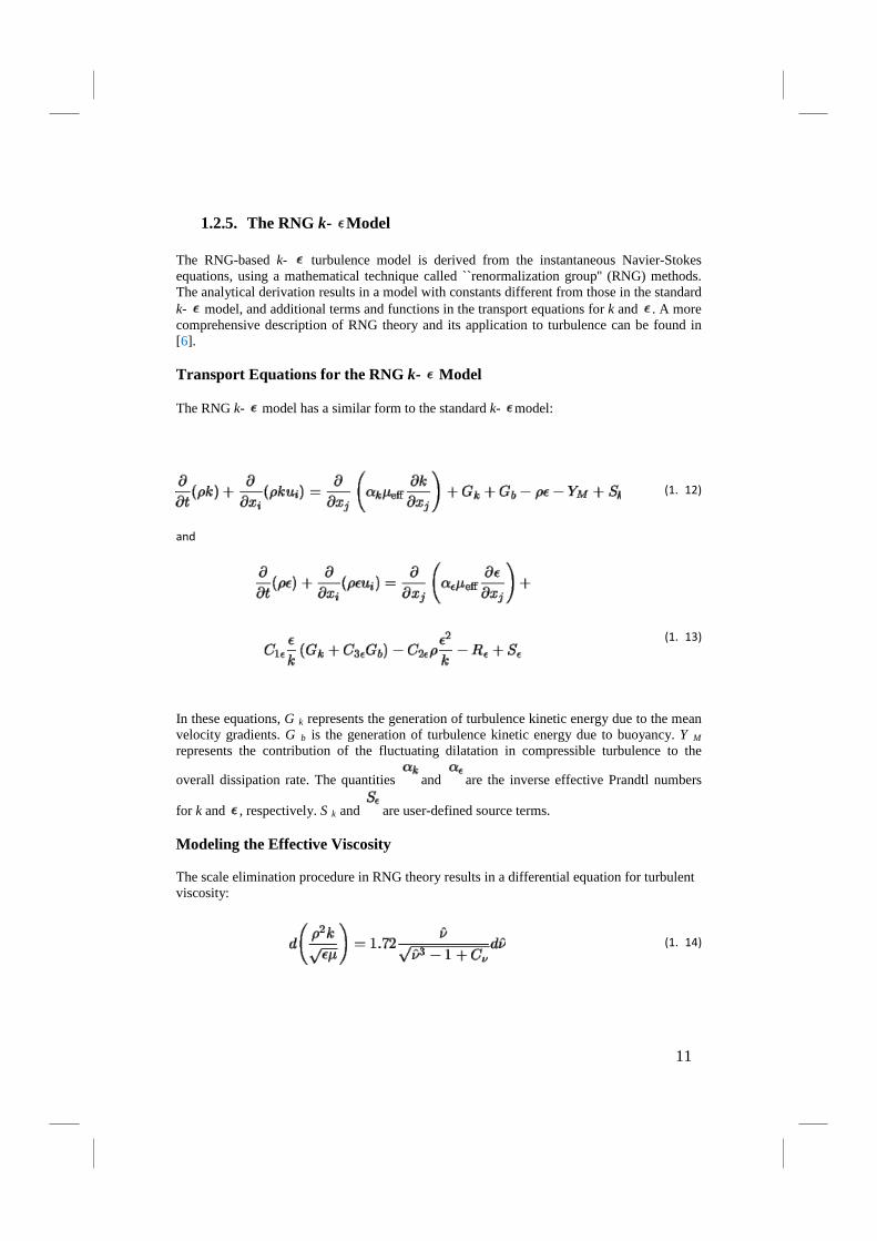
1.2.5. The RNG k- Model
The RNG-based k- turbulence model is derived from the instantaneous Navier-Stokes equations, using a mathematical technique called ``renormalization group'' (RNG) methods. The analytical derivation results in a model with constants different from those in the standard k- model, and additional terms and functions in the transport equations for k and . A more comprehensive description of RNG theory and its application to turbulence can be found in [6].
Transport Equations for the RNG k- Model
The RNG k-
model has a similar form to the standard k- model:
(1. 12)
and
(1. 13)
In these equations, G k represents the generation of turbulence kinetic energy due to the mean velocity gradients. G b is the generation of turbulence kinetic energy due to buoyancy. Y M represents the contribution of the fluctuating dilatation in compressible turbulence to the
overall dissipation rate. The quantities and are the inverse effective Prandtl numbers
for k and , respectively. S k and are user-defined source terms.
The scale elimination procedure in RNG theory results in a differential equation for turbulent viscosity:
Modeling the Effective Viscosity
(1. 14)
11

where
=
100
Equation (1. 14) is integrated to obtain an accurate description of how the effective turbulent transport varies with the effective Reynolds number (or eddy scale), allowing the model to better handle low-Reynolds-number and near-wall flows .
In the high-Reynolds-number limit, Equation (1. 14) gives
(1. 15)
with , derived using RNG theory. It is interesting to note that this value of
is very close to the empirically-determined value of 0.09 used in the standard k- model.
RNG Swirl Modification
Turbulence, in general, is affected by rotation or swirl in the mean flow. The RNG model in FLUENT provides an option to account for the effects of swirl or rotation by modifying the turbulent viscosity appropriately. The modification takes the following functional form:
(1. 16)
where is the value of turbulent viscosity calculated without the swirl modification using either Equation (1. 14) or Equation (1. 15). is a characteristic swirl number evaluated
within FLUENT, and is a swirl constant that assumes different values depending on whether the flow is swirl-dominated or only mildly swirling. This swirl modification always takes effect for axisymmetric, swirling flows and three-dimensional flows when the RNG
model is selected. For mildly swirling flows (the default in FLUENT), is set to 0.05 and
cannot be modified. For strongly swirling flows, however, a higher value of can be used.
12
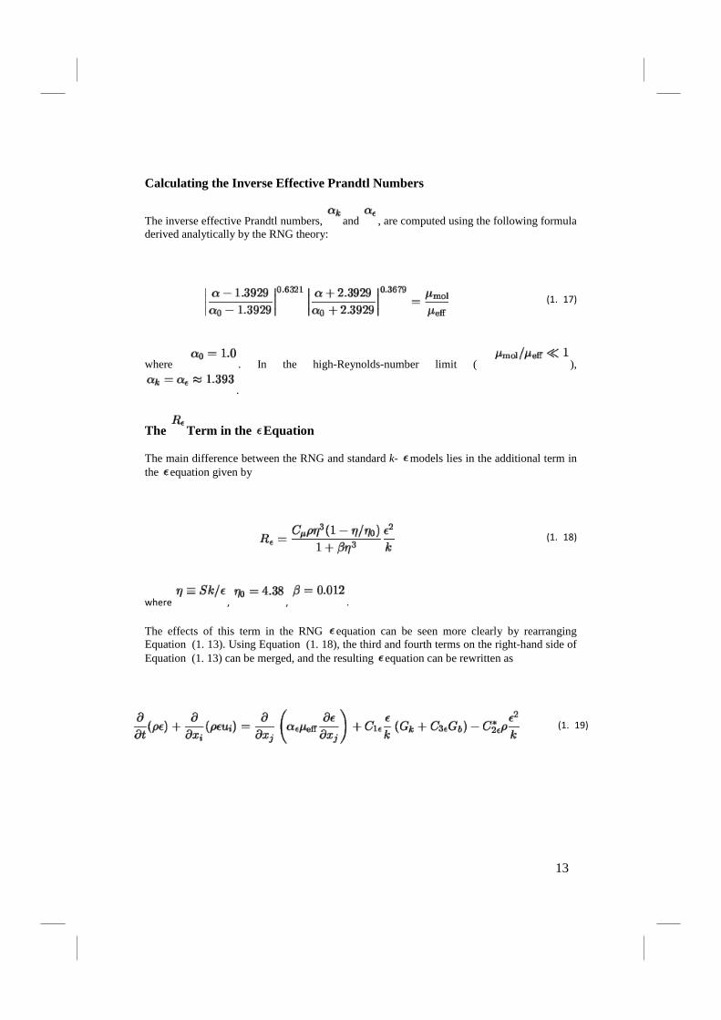
Calculating the Inverse Effective Prandtl Numbers
The inverse effective Prandtl numbers,
and , are computed using the following formula derived analytically by the RNG theory:
(1. 17)
where . In the high-Reynolds-number limit ( ),
.
The Term in the Equation
The main difference between the RNG and standard k-
models lies in the additional term in the equation given by
(1. 18)
where , , .
The effects of this term in the RNG equation can be seen more clearly by rearranging Equation (1. 13). Using Equation (1. 18), the third and fourth terms on the right-hand side of Equation (1. 13) can be merged, and the resulting equation can be rewritten as
(1. 19)
13
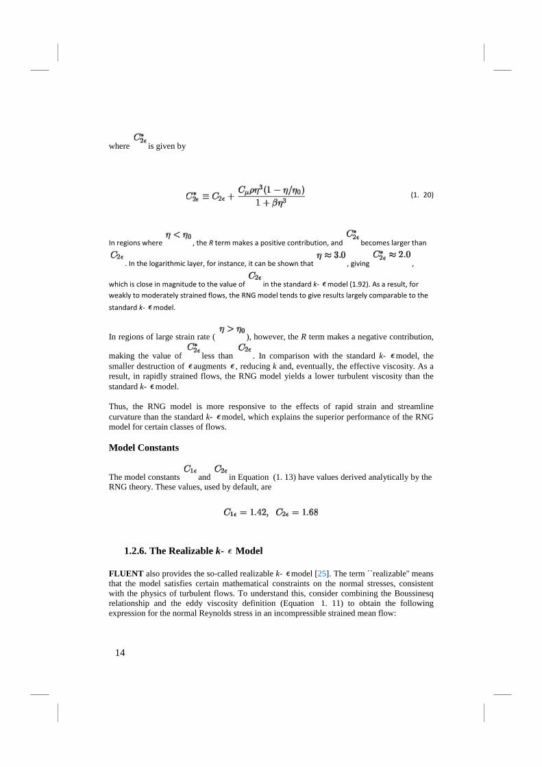
where is given by
(1. 20)
In regions where , the R term makes a positive contribution, and becomes larger than
. In the logarithmic layer, for instance, it can be shown that , giving ,
which is close in magnitude to the value of in the standard k- model (1.92). As a result, for weakly to moderately strained flows, the RNG model tends to give results largely comparable to the
standard k- model.
In regions of large strain rate ( ), however, the R term makes a negative contribution,
making the value of less than . In comparison with the standard k- model, the smaller destruction of augments , reducing k and, eventually, the effective viscosity. As a result, in rapidly strained flows, the RNG model yields a lower turbulent viscosity than the standard k- model.
Thus, the RNG model is more responsive to the effects of rapid strain and streamline curvature than the standard k- model, which explains the superior performance of the RNG model for certain classes of flows.
Model Constants
The model constants
and in Equation (1. 13) have values derived analytically by the RNG theory. These values, used by default, are
1.2.6. The Realizable k- Model
FLUENT also provides the so-called realizable k- model [25]. The term ``realizable'' means that the model satisfies certain mathematical constraints on the normal stresses, consistent with the physics of turbulent flows. To understand this, consider combining the Boussinesq relationship and the eddy viscosity definition (Equation 1. 11) to obtain the following expression for the normal Reynolds stress in an incompressible strained mean flow:
14

(1. 21)
Using Equation (1. 11) for , one obtains the result that the normal stress, , which by definition is a positive quantity, becomes negative, i.e., ``non-realizable'', when the strain is large enough to satisfy
(1. 22)
Similarly, it can also be shown that the Schwarz inequality for shear stresses
( ; no summation over and ) can be violated when the mean strain rate is large. The most straightforward way to ensure the realizability (positivity of normal stresses
and Schwarz inequality for shear stresses) is to make variable by sensitizing it to the mean
flow (mean deformation) and the turbulence ( k, ). The notion of variable is suggested by many modelers including Reynolds [ 24], and is well substantiated by experimental
evidence. For example, is found to be around 0.09 in the inertial sublayer of equilibrium boundary layers, and 0.05 in a strong homogeneous shear flow.
Another weakness of the standard k- model or other traditional k- models lies with the modeled equation for the dissipation rate ( ). The well-known round-jet anomaly (named based on the finding that the spreading rate in planar jets is predicted reasonably well, but prediction of the spreading rate for axisymmetric jets is unexpectedly poor) is considered to be mainly due to the modeled dissipation equation.
The realizable k- model proposed by Shih et al. [25] was intended to address these deficiencies of traditional k- models by adopting the following:
• a new eddy-viscosity formula involving a variable originally proposed by Reynolds
• a new model equation for dissipation ( ) based on the dynamic equation of the mean-square vorticity fluctuation
15
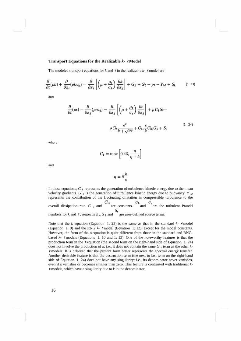
Transport Equations for the Realizable k- Model
The modeled transport equations for k and
in the realizable k- model are
(1. 23)
and
(1. 24)
where
and
In these equations, G k represents the generation of turbulence kinetic energy due to the mean velocity gradients. G b is the generation of turbulence kinetic energy due to buoyancy. Y M represents the contribution of the fluctuating dilatation in compressible turbulence to the
overall dissipation rate. C 2 and are constants. and are the turbulent Prandtl
numbers for k and , respectively. S k and are user-defined source terms.
Note that the k equation (Equation 1. 23) is the same as that in the standard k- model (Equation 1. 9) and the RNG k- model (Equation 1. 12), except for the model constants. However, the form of the equation is quite different from those in the standard and RNG-based k- models (Equations 1. 10 and 1. 13). One of the noteworthy features is that the production term in the equation (the second term on the right-hand side of Equation 1. 24) does not involve the production of k; i.e., it does not contain the same G k term as the other k-
models. It is believed that the present form better represents the spectral energy transfer. Another desirable feature is that the destruction term (the next to last term on the right-hand side of Equation 1. 24) does not have any singularity; i.e., its denominator never vanishes, even if k vanishes or becomes smaller than zero. This feature is contrasted with traditional k-
models, which have a singularity due to k in the denominator.
16

This model has been extensively validated for a wide range of flows [ 15, 25], including rotating homogeneous shear flows, free flows including jets and mixing layers, channel and boundary layer flows, and separated flows. For all these cases, the performance of the model has been found to be substantially better than that of the standard k- model. Especially noteworthy is the fact that the realizable k- model resolves the round-jet anomaly; i.e., it predicts the spreading rate for axisymmetric jets as well as that for planar jets.
Modeling the Turbulent Viscosity
As in other k-
models, the eddy viscosity is computed from
(1. 25)
The difference between the realizable k- model and the standard and RNG k- models is
that is no longer constant. It is computed from
(1. 26)
where
(1. 27)
and
(1. 28)
(1. 29)
where is the mean rate-of-rotation tensor viewed in a rotating reference frame with the
angular velocity . The model constants A 0 and A s are given by
17

where
(1. 30)
It can be seen that is a function of the mean strain and rotation rates, the angular velocity
of the system rotation, and the turbulence fields ( k and ). in (Equation 1. 25) can be shown to recover the standard value of 0.09 for an inertial sublayer in an equilibrium boundary layer.
Model Constants
The model constants C
2, , and have been established to ensure that the model performs well for certain canonical flows. The model constants are
1.2.7. The Standard and SST k- Models
This section presents the standard and shear-stress transport (SST) k- models. Both models have similar forms, with transport equations for k and . The major ways in which the SST model differs from the standard model are as follows:
• gradual change from the standard k- model in the inner region of the boundary layer to a high-Reynolds-number version of the k- model in the outer part of the boundary layer
• modified turbulent viscosity formulation to account for the transport effects of the principal turbulent shear stress
The transport equations, methods of calculating turbulent viscosity, and methods of calculating model constants and other terms are presented separately for each model.
18

1.2.8. The Standard k- Model
The standard k - model is an empirical model based on model transport equations for the turbulence kinetic energy ( k) and the specific dissipation rate ( ), which can also be thought of as the ratio of to k [29].
As the k- model has been modified over the years, production terms have been added to both the k and equations, which have improved the accuracy of the model for predicting free shear flows.
Transport Equations for the Standard k- Model
The turbulence kinetic energy, k, and the specific dissipation rate,
, are obtained from the following transport equations:
(1. 31)
and
(1. 32)
In these equations, G k represents the generation of turbulence kinetic energy due to mean
velocity gradients. represents the generation of . and represent the effective
diffusivity of k and , respectively. Y k and represent the dissipation of k and due to
turbulence. All of the above terms are calculated as described below. S k and are user-defined source terms.
Modeling the Effective Diffusivity
The effective diffusivities for the k-
model are given by
=
(1. 33)
=
(1. 34)
19
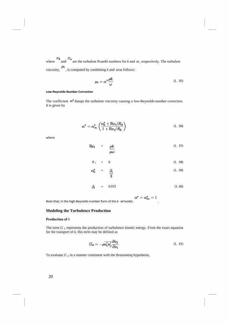
where and are the turbulent Prandtl numbers for k and , respectively. The turbulent
viscosity, , is computed by combining k and as follows:
(1. 35)
Low-Reynolds-Number Correction
The coefficient damps the turbulent viscosity causing a low-Reynolds-number correction. It is given by
(1. 36)
where
=
(1. 37)
R = k 6 (1. 38)
=
(1. 39)
= 0.072 (1. 40)
Note that, in the high-Reynolds-number form of the k- model, .
Modeling the Turbulence Production
Production of k
The term G k represents the production of turbulence kinetic energy. From the exact equation for the transport of k, this term may be defined as
(1. 41)
To evaluate G k in a manner consistent with the Boussinesq hypothesis,
20
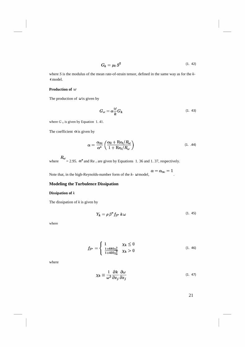
(1. 42)
where S is the modulus of the mean rate-of-strain tensor, defined in the same way as for the k- model.
Production of
The production of is given by
(1. 43)
where G k
The coefficient
is given by Equation 1. 41.
is given by
(1. .44)
where = 2.95. and Re t
Note that, in the high-Reynolds-number form of the k-
are given by Equations 1. 36 and 1. 37, respectively.
model, .
Modeling the Turbulence Dissipation
Dissipation of k
The dissipation of k is given by
(1. 45)
where
(1. 46)
where
(1. 47)
21
and
=
(1. 48)
=
(1. 49)
= 1.5 (1. 50)
= 8 (1. 51)
= 0.09 (1. 52)
where Re t
Dissipation of
is given by Equation 1. 37
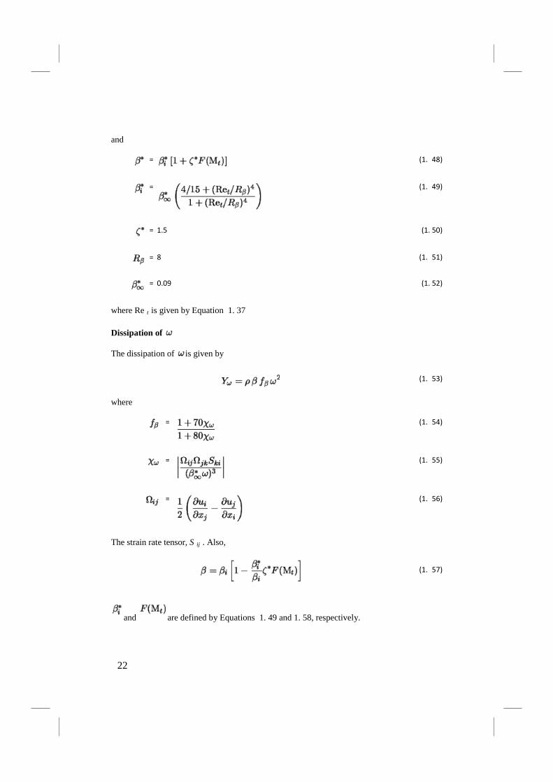
The dissipation of is given by
(1. 53)
where
=
(1. 54)
=
(1. 55)
=
(1. 56)
The strain rate tensor, S ij . Also,
(1. 57)
and are defined by Equations 1. 49 and 1. 58, respectively.
22

Compressibility Correction
The compressibility function, , is given by
(1. 58)
where
(1. 59)
= 0.25 (1. 60)
a =
(1. 61)
Note that, in the high-Reynolds-number form of the k- model, . In the incompressible
form, .
Model Constants
Wall Boundary Conditions
The wall boundary conditions for the k equation in the k-
models are treated in the same way as the k equation is treated when enhanced wall treatments are used with the k- models. This means that all boundary conditions for wall-function meshes will correspond to the wall function approach, while for the fine meshes, the appropriate low-Reynolds-number boundary conditions will be applied.
In FLUENT the value of at the wall is specified as
23
(1. 62)
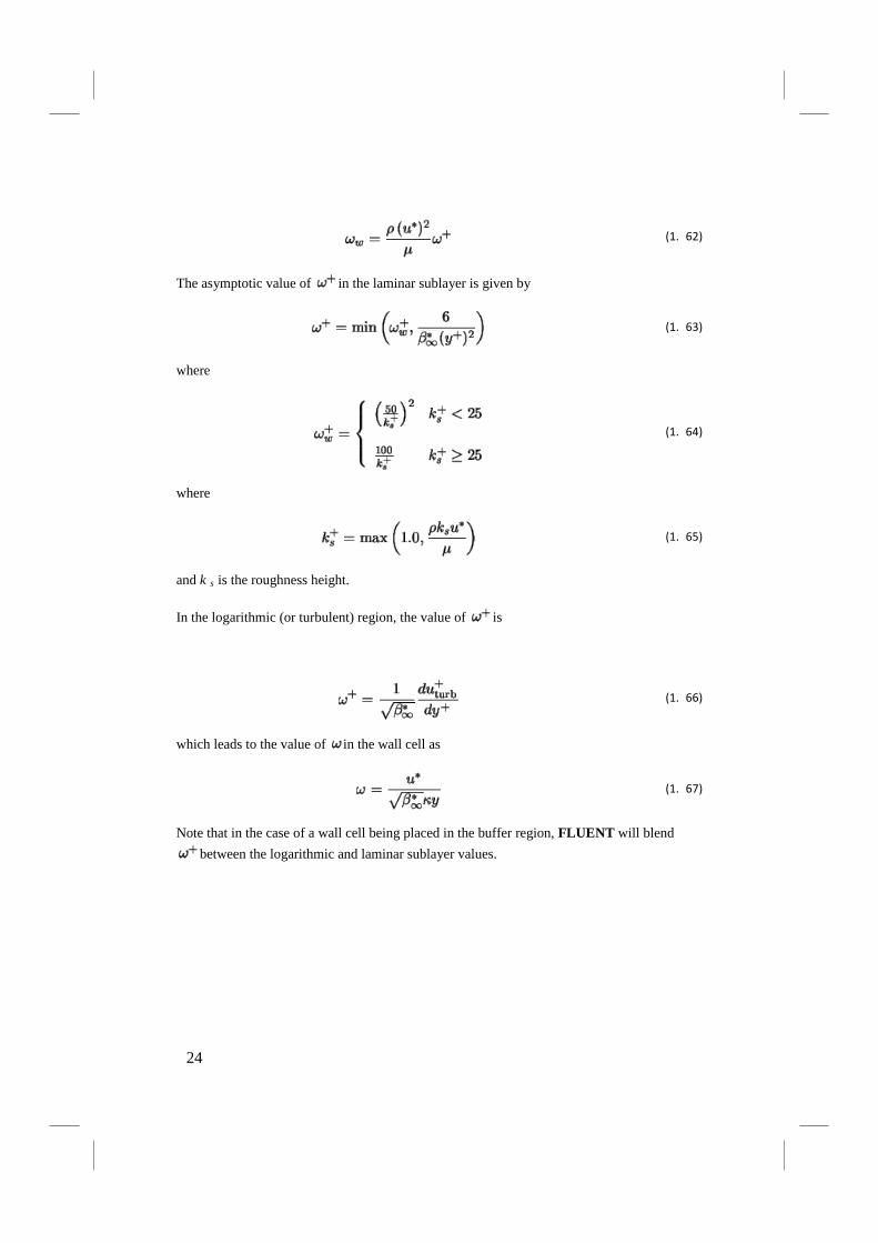
The asymptotic value of in the laminar sublayer is given by
(1. 63)
where
(1. 64)
where
(1. 65)
and k s
In the logarithmic (or turbulent) region, the value of
is the roughness height.
is
(1. 66)
which leads to the value of in the wall cell as
(1. 67)
Note that in the case of a wall cell being placed in the buffer region, FLUENT will blend between the logarithmic and laminar sublayer values.
24

1.2.9. The Reynolds Stress Transport Equations
The exact transport equations for the transport of the Reynolds stresses, , may be written as follows:
(1. 68)
Of the various terms in these exact equations, C ij, D L, ij, P ij, and F ij do not require any
modeling. However, D T, ij, G ij, , and need to be modeled to close the equations. The following sections describe the modeling assumptions required to close the equation set.
1.3. Solution Strategies for Turbulent Flow Simulations
Compared to laminar flows, simulations of turbulent flows are more challenging in many ways. For the Reynolds-averaged approach, additional equations are solved for the turbulence
quantities. Since the equations for mean quantities and the turbulent quantities ( , k, , , or the Reynolds stresses) are strongly coupled in a highly non-linear fashion, it takes more
25
computational effort to obtain a converged turbulent solution than to obtain a converged laminar solution. The LES model, while embodying a simpler, algebraic model for the subgrid-scale viscosity, requires a transient solution on a very fine mesh.
The fidelity of the results for turbulent flows is largely determined by the turbulence model being used. Here are some guidelines that can enhance the quality of your turbulent flow simulations.
1.4. Mesh Generation
The following are suggestions to follow when generating the mesh for use in your turbulent flow simulation:
• Picture in your mind the flow under consideration using your physical intuition or any data for a similar flow situation, and identify the main flow features expected in the flow you want to model. Generate a mesh that can resolve the major features that you expect.
• If the flow is wall-bounded, and the wall is expected to significantly affect the flow, take additional care when generating the mesh. You should avoid using a mesh that is too fine (for the wall function approach).
1.5. Accuracy
The suggestions below are provided to help you obtain better accuracy in your results:
• Use the turbulence model that is better suited for the salient features you expect to see in the flow
• Because the mean quantities have larger gradients in turbulent flows than in laminar flows, it is recommended that you use high-order schemes for the convection terms. This is especially true if you employ a triangular or tetrahedral mesh. Note that excessive numerical diffusion adversely affects the solution accuracy, even with the most elaborate turbulence model.
• In some flow situations involving inlet boundaries, the flow downstream of the inlet is dictated by the boundary conditions at the inlet. In such cases, you should exercise care to make sure that reasonably realistic boundary values are specified.
1.6. Convergence
The suggestions below are provided to help you enhance convergence for turbulent flow calculations:
• Starting with excessively crude initial guesses for mean and turbulence quantities may cause the solution to diverge. A safe approach is to start your calculation using conservative (small) under-relaxation parameters and (for the coupled solvers) a conservative Courant number, and increase them gradually as the iterations proceed and the solution begins to settle down.
• It is also helpful for faster convergence to start with reasonable initial guesses for the k and (or k and ) fields. Particularly when the enhanced wall treatment is used, it is
26
important to start with a sufficiently developed turbulence field, to avoid the need for an excessive number of iterations to develop the turbulence field.
• When you are using the RNG k- model, an approach that might help you achieve better convergence is to obtain a solution with the standard k- model before switching to the RNG model. Due to the additional non-linearities in the RNG model, lower under-relaxation factors and (for the coupled solvers) a lower Courant number might also be necessary.
Note that when you use the enhanced wall treatment, you may sometimes find during the calculation that the residual for is reported to be zero. This happens when your flow is such that Re y is less than 200 in the entire flow domain, and is obtained from the algebraic formula instead of from its transport equation.
27
22.. AAEERROODDYYNNAAMMIICCSS Simulation of flow around a vehicle is based on usage of basic function of software described in chapter 1. The procedures of computational data entering consist on development of geometry of the considered object, establishment of boundary conditions and the turbulences models selection, etc.
This problem will be explained with aid of example of flow around a vehicle that corresponds to the teaching materials of this course.
Introduction
The purpose of this tutorial is to compute the turbulent flow. You will use the Spalart-Allmaras turbulence model.
In this tutorial you will learn how to:
• Model an incompressible flow. • Set boundary conditions for external aerodynamics. • Use the Spalart-Allmaras turbulence model. • Calculate a solution using the coupled implicit solver. • Use force and surface monitors to check solution convergence.
Problem Description
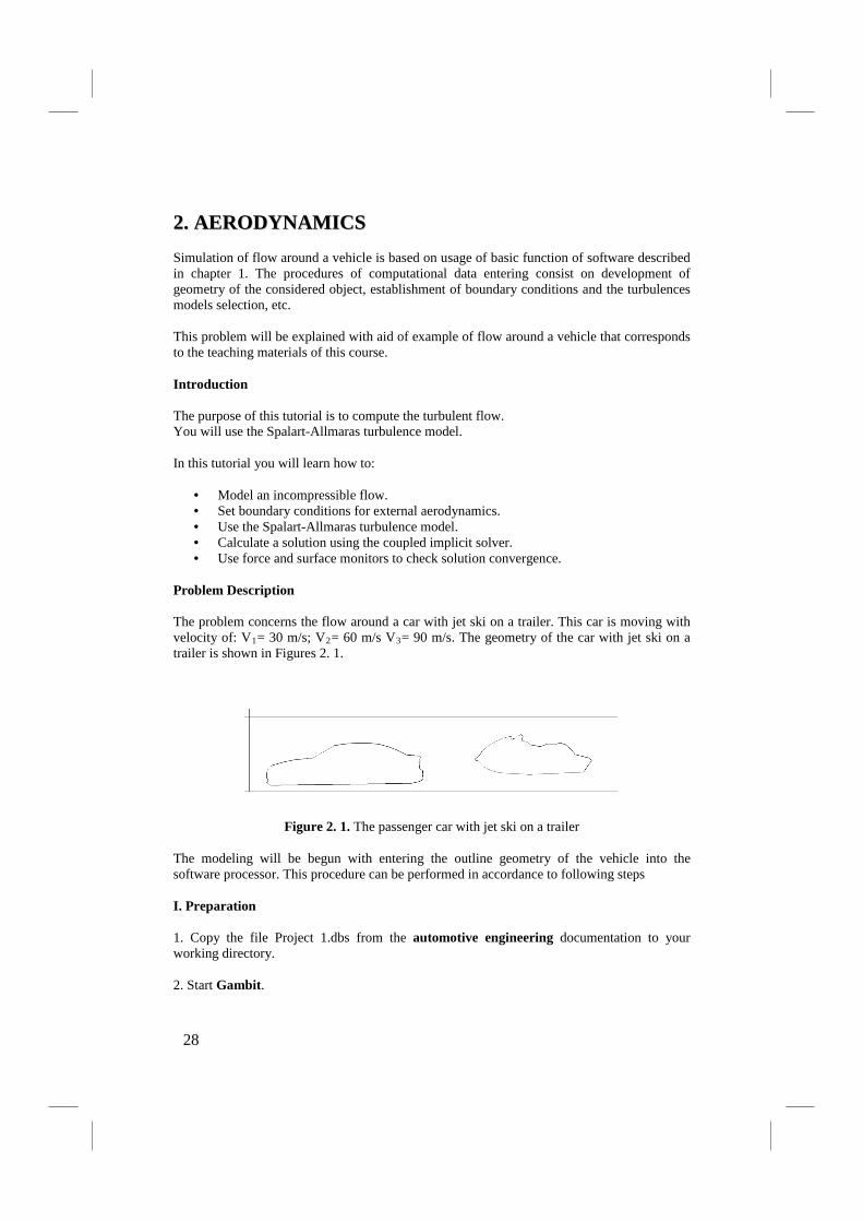
The problem concerns the flow around a car with jet ski on a trailer. This car is moving with velocity of: V1= 30 m/s; V2= 60 m/s V3
= 90 m/s. The geometry of the car with jet ski on a trailer is shown in Figures 2. 1.
Figure 2. 1. The passenger car with jet ski on a trailer
The modeling will be begun with entering the outline geometry of the vehicle into the software processor. This procedure can be performed in accordance to following steps
I. Preparation
1. Copy the file Project 1.dbs from the automotive engineering documentation to your working directory.
2. Start Gambit.
28
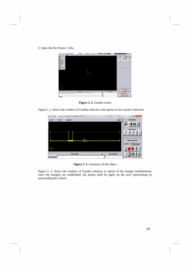
3. Open the file Project 1.dbs
Figure 2. 2. Gambit screes
Figure 2. 2. shows the window of Gambit software with option of new project selection.
Figure 2. 3. Geometry of the object
Figure 2. 3. shows the window of Gambit software in option of the margin establishment. Once the margins are established, the planes shall be apply on the area representing air surrounding the vehicle
29
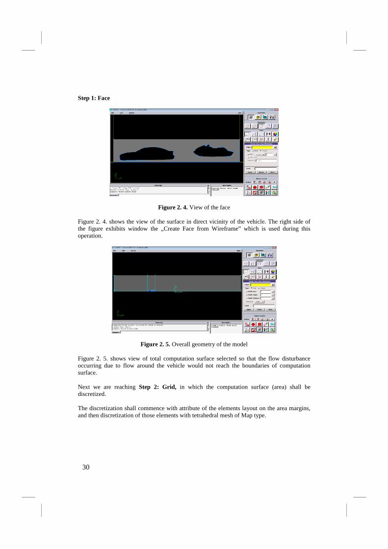
Step 1: Face
Figure 2. 4. View of the face
Figure 2. 4. shows the view of the surface in direct vicinity of the vehicle. The right side of the figure exhibits window the „Create Face from Wireframe” which is used during this operation.
Figure 2. 5. Overall geometry of the model
Figure 2. 5. shows view of total computation surface selected so that the flow disturbance occurring due to flow around the vehicle would not reach the boundaries of computation surface.
Next we are reaching Step 2: Grid, in which the computation surface (area) shall be discretized.
The discretization shall commence with attribute of the elements layout on the area margins, and then discretization of those elements with tetrahedral mesh of Map type.
30
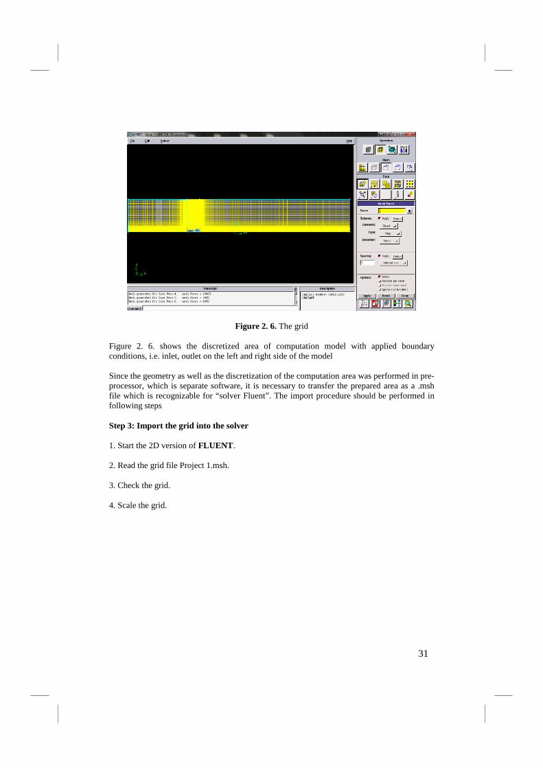
Figure 2. 6. The grid
Figure 2. 6. shows the discretized area of computation model with applied boundary conditions, i.e. inlet, outlet on the left and right side of the model
Since the geometry as well as the discretization of the computation area was performed in pre-processor, which is separate software, it is necessary to transfer the prepared area as a .msh file which is recognizable for “solver Fluent”. The import procedure should be performed in following steps
Step 3: Import the grid into the solver
1. Start the 2D version of FLUENT.
2. Read the grid file Project 1.msh.
3. Check the grid.
4. Scale the grid.
31

Figure 2. 7. Fluent read window
Figure 2. 7. shows the window of Fluent software with active menu of file selection.
Figure 2. 8. Scale window
Next the scale of imported surface Figure 2. 8. should be selected.
The selection procedure comprises following steps:
Step 4: Models
1. Select the Coupled, Implicit solver. 2. Select the k-epsilon model
32
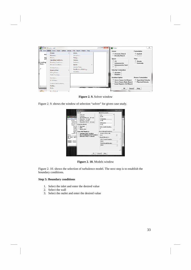
Figure 2. 9. Solver window
Figure 2. 9. shows the window of selection “solver” for given case study.
Figure 2. 10. Models window
Figure 2. 10. shows the selection of turbulence model. The next step is to establish the boundary conditions.
Step 5: Boundary conditions
1. Select the inlet and enter the desired value 2. Select the wall 3. Select the outlet and enter the desired value
33
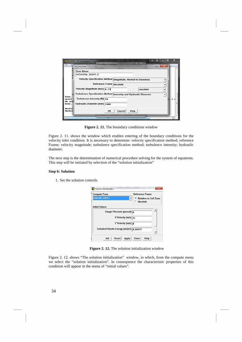
Figure 2. 11. The boundary conditions window
Figure 2. 11. shows the window which enables entering of the boundary conditions for the velocity inlet condition. It is necessary to determine: velocity specification method; reference Frame; velocity magnitude; turbulence specification method; turbulence intensity; hydraulic diameter.
The next step is the determination of numerical procedure solving for the system of equations. This step will be initiated by selection of the “solution initialization”
Step 6: Solution
1. Set the solution controls.
Figure 2. 12. The solution initialization window
Figure 2. 12. shows “The solution initialization” window, in which, from the compute menu we select the “solution initialization”. In consequence the characteristic properties of this condition will appear in the menu of “initial values”.
34
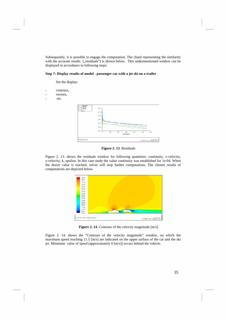
Subsequently, it is possible to engage the computation. The chard representing the similarity with the accurate results („residuals”) is shown below. This undermentioned window can be displayed in accordance to following steps:
Step 7: Display results of model - passenger car with a jet ski on a trailer
Set the display:
- contours, - vectors, - etc.
Figure 2. 13. Residuals
Figure 2. 13. shows the residuals window for following quantities: continuity, x-velocity, y-velocity, k, epsilon. In this case study the value continuity was established for 1e-04. When the desire value is reached, solver will stop farther computations. The chosen results of computations are depicted below.
Figure 2. 14. Contours of the velocity magnitude [m/s]
Figure 2. 14. shows the “Contours of the velocity magnitude” window, on which the maximum speed reaching 11.5 [m/s] are indicated on the upper surface of the car and the ski jet. Minimum value of speed (approximately 0 [m/s]) occurs behind the vehicle.
35
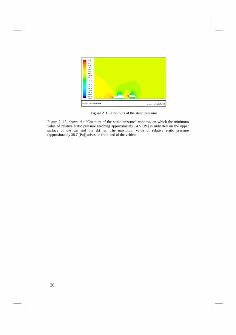
Figure 2. 15. Contours of the static pressure
Figure 2. 15. shows the “Contours of the static pressure” window, on which the minimum value of relative static pressure reaching approximately 34.5 [Pa] is indicated on the upper surface of the car and the ski jet. The maximum value of relative static pressure (approximately 38.7 [Pa]) arises on front-end of the vehicle.
36
33.. IINNLLEETT AANNDD OOUUTTLLEETT IINN CCOOMMBBUUSSTTIIOONN EENNGGIINNEESS
Introduction
A piston combustion engine is a heat engine (a thermodynamic one), in which the chemical energy of the fuel is transferred into thermal energy, and this in turn is transferred into the mechanical energy.
Obtaining best performance characteristics of the combustion engine was one of the highest priority since the very beginning of their existence. Initially however, the emphasis was given on increasing power and total efficiency of an engine. As the time goes by the requirements become more sophisticated and starts to concern greater number of working parameters of an engine. the essential issue however, remains the improvement of the cylinder filling process.
Latest procedures for combustion engine cylinder filling, which considers the influence of an intake system can be comprised into the determination of flow resistance as well as the vibration of the column of gas within the intake system, by means of numerical computation software, i.e. CFD (Computational Fluid Dynamics). The CFD software are mostly based on the Finite Element Method (FEM) [1], [31], [33] or on the Finite Volume Method (FVM) [18], [30]. Those software are capable of pressure and velocity fields determination which arises during the medium flow through the intake system. Furthermore, such software allows the flow expertise when geometry, friction on the ducts walls, viscosity of the medium, and heat transfer are taken into consideration. In order to perform the computation, it is necessary to design the numerical shape of the intake system, and then this model should be discretized for instance with aid of Gambit software [13]. For such prepared model the boundary and initial conditions should be established and the computational condition should be selected. The CFD methods are relatively cheap, despise of course the cost of the software. Some parameters which characterizes the flow are determined with higher accuracy comparing with the comparative methods. For example measuring velocity field or pressure distribution is theoretically possible but not used in practice due to their high cost.
correct preparation of the mesh as well as establishment of certain initial and boundary conditions, and selection of necessary computation parameters requires following established procedure [1], [2], [7], [53] and some experience. The computation time of a stationary flow is relatively short. On available computers the computations can last for several hours in case of air intake of the combustion engine. The nonstationary computation (with consideration of total intake stroke) can last even for several days. However taking the rapid development of computer equipment it is safe to assume that this method will be more universal. Presently, there are many computation software, however data exchange between them is rather problematic. In case of CFD the interpretation of data seems to be the most problematic. “A computer will calculate everything”. Unfortunately, computer very rarely is able to consider the physical quantity of the phenomenon. All computation presented in this work was
37
performed using FLUENT software, which is considered as one of the best commercial software.
The computation od the intace system wlle be presented on the undermentioned example.
Problem Description
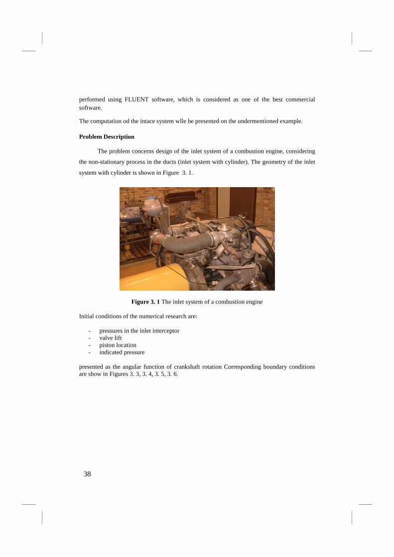
The problem concerns design of the inlet system of a combustion engine, considering
the non-stationary process in the ducts (inlet system with cylinder). The geometry of the inlet
system with cylinder is shown in Figure 3. 1.
Figure 3. 1 The inlet system of a combustion engine
Initial conditions of the numerical research are:
- pressures in the inlet interceptor - valve lift - piston location - indicated pressure
presented as the angular function of crankshaft rotation Corresponding boundary conditions are show in Figures 3. 3, 3. 4, 3. 5, 3. 6.
38
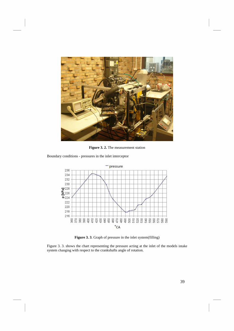
Figure 3. 2. The measurement station
Boundary conditions - pressures in the inlet interceptor
Figure 3. 3. Graph of pressure in the inlet system(filling)
Figure 3. 3. shows the chart representing the pressure acting at the inlet of the models intake system changing with respect to the crankshafts angle of rotation.
39
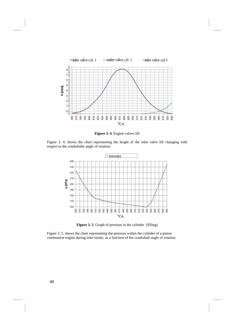
Figure 3. 4. Engine valves lift
Figure 3. 4. shows the chart representing the height of the inlet valve lift changing with respect to the crankshafts angle of rotation.
Figure 3. 5. Graph of pressure in the cylinder (filling)
Figure 3. 5. shows the chart representing the pressure within the cylinder of a piston combustion engine during inlet stroke, as a function of the crankshaft angle of rotation.
40
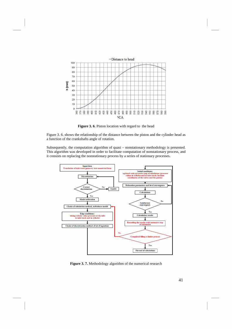
Figure 3. 6. Piston location with regard to the head
Figure 3. 6. shows the relationship of the distance between the piston and the cylinder head as a function of the crankshafts angle of rotation.
Subsequently, the computation algorithm of quasi – nonstationary methodology is presented. This algorithm was developed in order to facilitate computation of nonstationary process, and it consists on replacing the nonstationary process by a series of stationary processes.
Figure 3. 7. Methodology algorithm of the numerical research
41
The computation should be performed in accordance with following steps:
Step 1: Preparation
1. Copy the file Project II.msh from the automotive engineering documentation to your working directory.
Step 2: Read Grid in Solver
1. Start the 3D version of FLUENT.
2. Read the grid file Project II.msh.
3. Check the grid.
4. Scale the grid.
5. Display the grid
Step 4: Models
1. Select the Coupled, Implicit solver. 2. Select the k-epsilon model
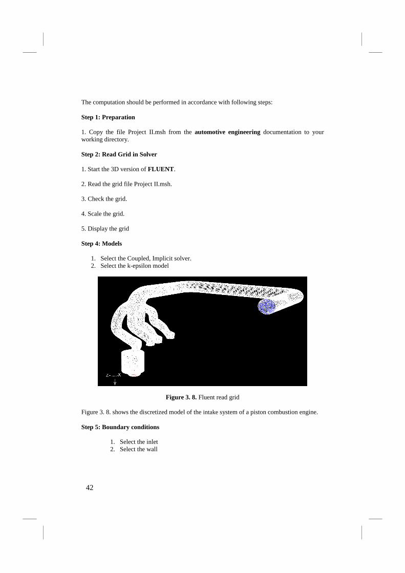
Figure 3. 8. Fluent read grid
Figure 3. 8. shows the discretized model of the intake system of a piston combustion engine.
Step 5: Boundary conditions
1. Select the inlet 2. Select the wall
42

Figure 3. 9. Model of the inlet system‘s geometry with boundary conditions
Figure 3. 9. shows the intake system of a piston combustion engine with established boundary conditions, i.e. inlet and outlet.
Step 6: Solution
1. Set the solution controls.
Figure 3. 10. The boundary conditions window
Figure 3. 10. shows “The solution initialization” window, in which, from the “compute” menu we select the “solution initialization”. In consequence the characteristic properties of this condition will appear in the menu of ‘initial values”
The computation has been performed and Results of the numerical research are presented in undermentioned step 7.
Step 7: Set: display vectors.
43
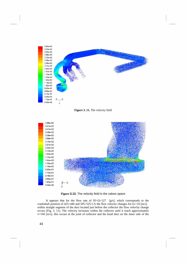
Figure 3. 11. The velocity field
Figure 3.12. The velocity field in the valves space
It appears that for the flow rate of 95<Q<127 [g/s], which corresponds to the crankshaft position of 425÷440 and 505÷525 CA the flow velocity changes for Δv=10 [m/s]. within straight segment of the duct located just before the collector the flow velocity change occurs (Fig. 3. 11). The velocity increases within the collector until it reach approximately v≈160 [m/s]. this occurs at the joint of collector and the head duct on the inner side of the
44
curve. The velocity farther decreases. When the flow however reach the helical segment of the system, the velocity will increase again until the speed similar to the one in inner side of the curve i.e. v≈160 [m/s] (Fig. 3. 12). Significant increase of the velocity can be observed at the valve port. The velocity exceeds the speed of sound on the negligible space.
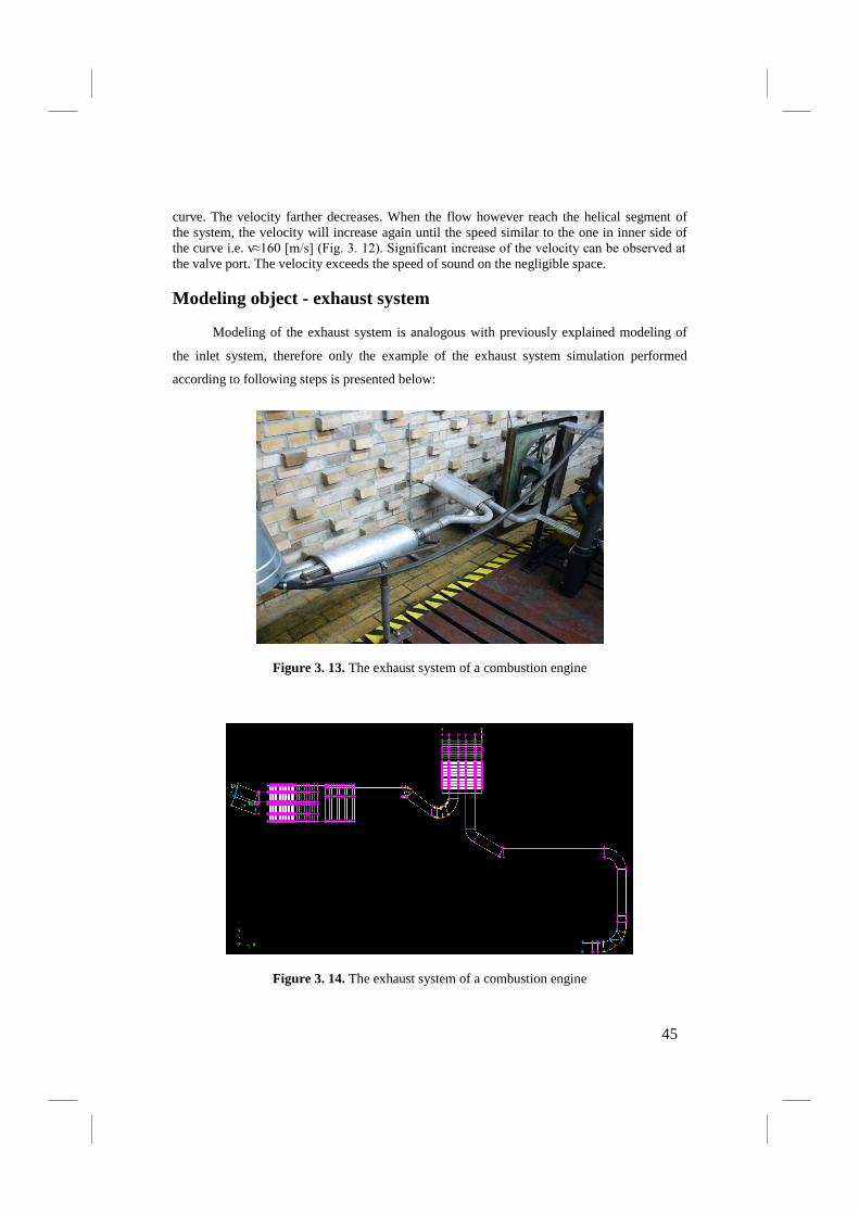
Modeling object - exhaust system
Modeling of the exhaust system is analogous with previously explained modeling of
the inlet system, therefore only the example of the exhaust system simulation performed
according to following steps is presented below:
Figure 3. 13. The exhaust system of a combustion engine
Figure 3. 14. The exhaust system of a combustion engine
45
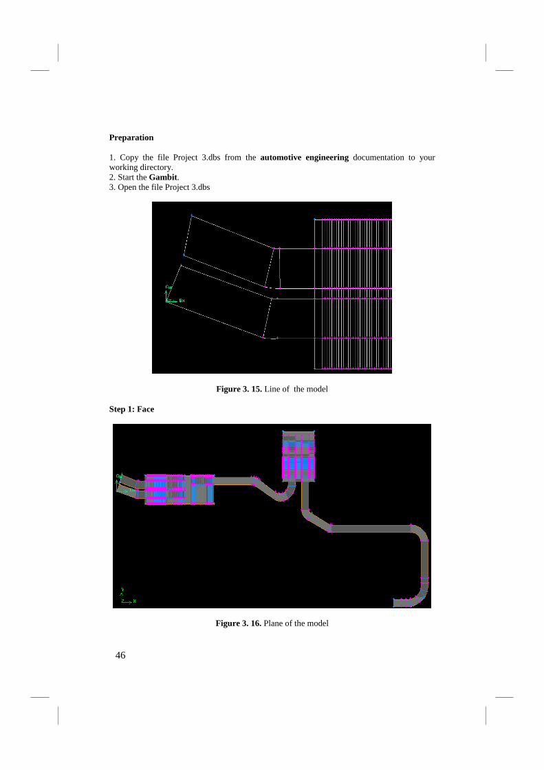
Preparation
1. Copy the file Project 3.dbs from the automotive engineering documentation to your working directory. 2. Start the Gambit. 3. Open the file Project 3.dbs
Figure 3. 15. Line of the model
Step 1: Face
Figure 3. 16. Plane of the model
46
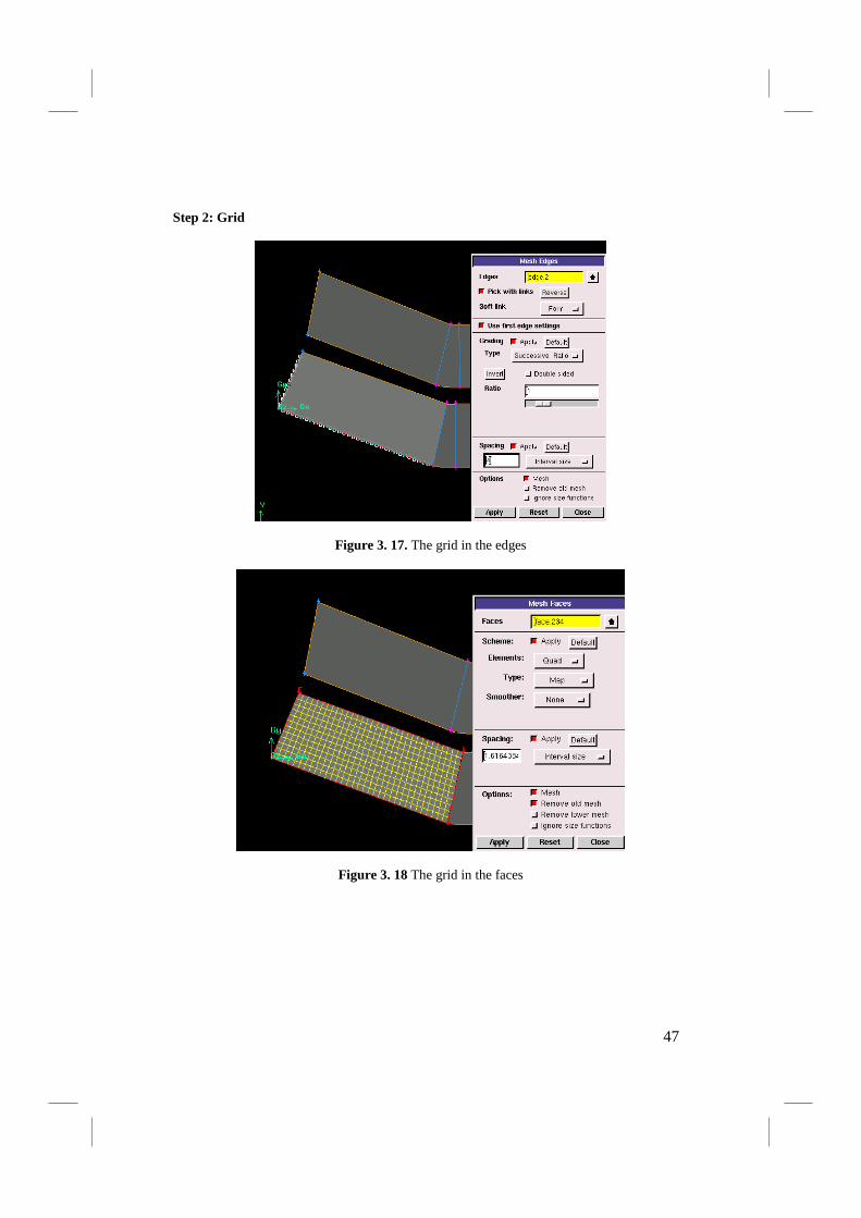
Step 2: Grid
Figure 3. 17. The grid in the edges
Figure 3. 18 The grid in the faces
47
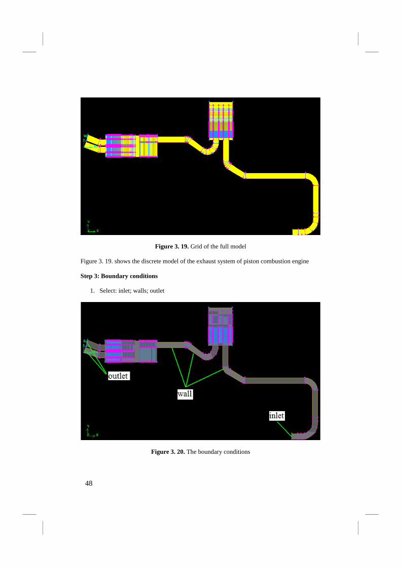
Figure 3. 19. Grid of the full model
Figure 3. 19. shows the discrete model of the exhaust system of piston combustion engine
Step 3: Boundary conditions
1. Select: inlet; walls; outlet
Figure 3. 20. The boundary conditions
48
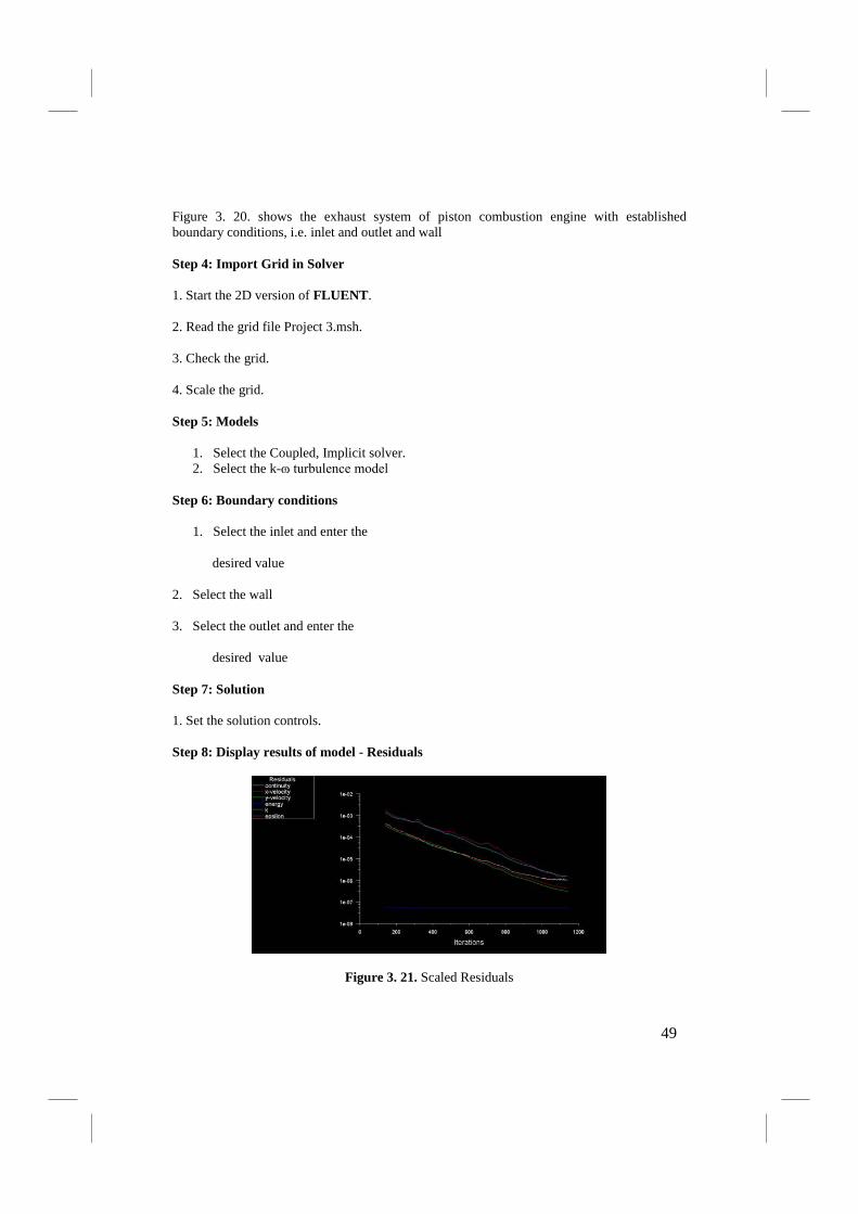
Figure 3. 20. shows the exhaust system of piston combustion engine with established boundary conditions, i.e. inlet and outlet and wall
Step 4: Import Grid in Solver
1. Start the 2D version of FLUENT.
2. Read the grid file Project 3.msh.
3. Check the grid.
4. Scale the grid.
Step 5: Models
1. Select the Coupled, Implicit solver. 2. Select the k-ɷ turbulence model
Step 6: Boundary conditions
1. Select the inlet and enter the
desired value
2. Select the wall
3. Select the outlet and enter the
desired value
Step 7: Solution
1. Set the solution controls.
Step 8: Display results of model - Residuals
Figure 3. 21. Scaled Residuals
49

Figure 3. 21. shows the “residuals” window for following quantities: continuity, x-velocity, y-velocity, k, epsilon. In this case study the value continuity was established for 1e-05. When the desire value is reached, solver will stop farther computations. The chosen results of computations are depicted below.
Step 8: Display results of model – exhaust system
Set : display contours of velocity,
Figure 3. 22. Velocity Magnitude [m/s]
Figure 3. 22. shows the velocity field of the gas. Minimum velocity occurs in the muffler chambers (approximately 0.01 [m/s]) whereas the maximum velocity (approximately 12.4 [m/s]) occurs on the inner side of the systems duct elbows.
Step 8: Display results of model – exhaust system
Set: display contours of pressure,
Figure 3. 23. Total Pressure (Pa)
Figure 3. 23. shows the pressure distribution inside the muffler for the velocity of 8m/s. The gas decompresses within the muffler. Maximum pressure occurs at the outlet, i.e. 2hPa
50
44.. MMOOVVIINNGG//DDEEFFOORRMMIINNGG MMEESSHH [[1144]] In sliding meshes, the relative motion of stationary and rotating components in a rotating machine will give rise to unsteady interactions. The dynamic mesh model is used when boundaries move rigidly (linear or rotating) with respect to each other. For example
• A piston moving with respect to an engine cylinder. • A ap moving with respect to an airplane wing.
The dynamic mesh model can also be used when boundaries deform or defect. For example • A balloon that is being inflated. • An artificial wall responding to the pressure pulse from the heart.
4.1. Conservation Equations
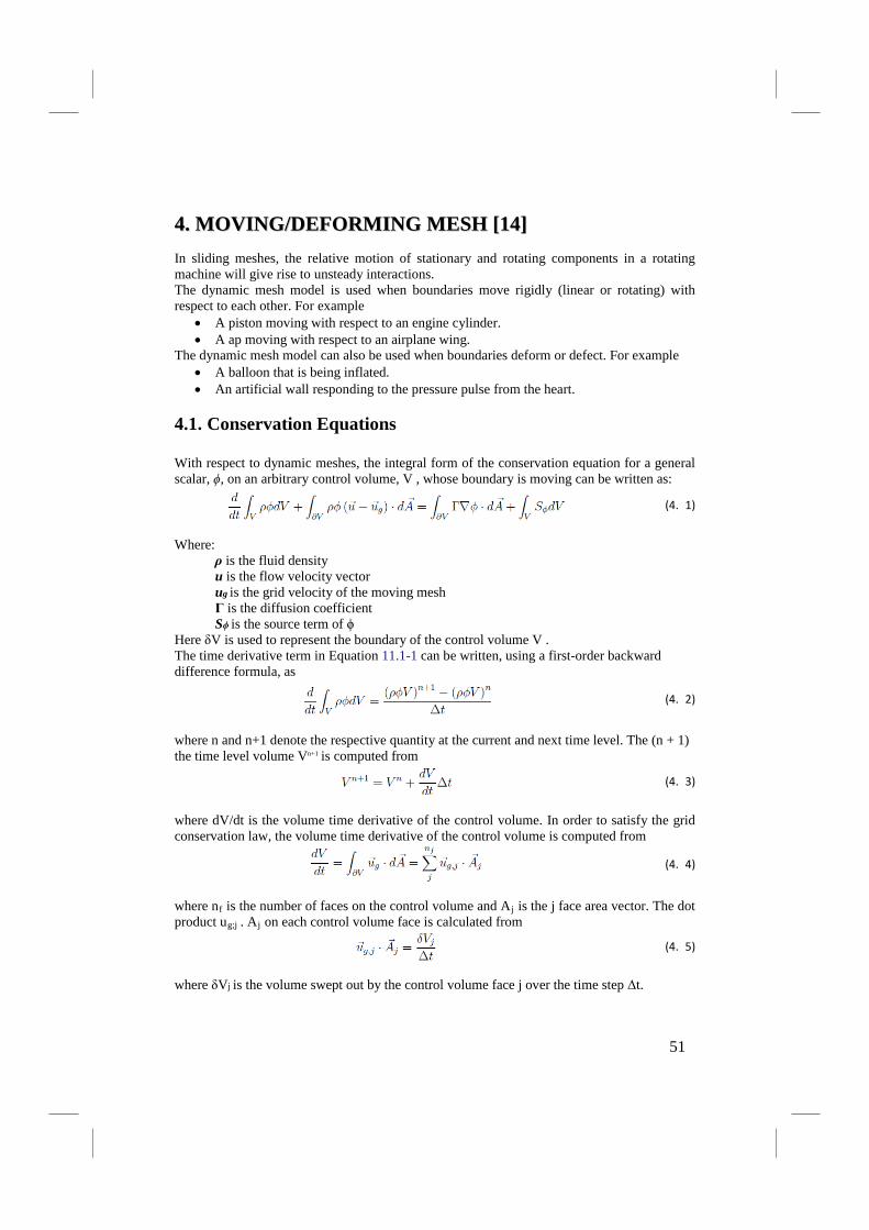
With respect to dynamic meshes, the integral form of the conservation equation for a general scalar, ϕ, on an arbitrary control volume, V , whose boundary is moving can be written as:
(4. 1)
Where: ρ is the fluid density u is the flow velocity vector ug is the grid velocity of the moving mesh Γ is the diffusion coefficient Sϕ is the source term of ϕ
Here δV is used to represent the boundary of the control volume V . The time derivative term in Equation 11.1-1 can be written, using a first-order backward difference formula, as
(4. 2)
where n and n+1 denote the respective quantity at the current and next time level. The (n + 1) the time level volume Vn+1 is computed from
(4. 3)
where dV/dt is the volume time derivative of the control volume. In order to satisfy the grid conservation law, the volume time derivative of the control volume is computed from
(4. 4)
where nf is the number of faces on the control volume and Aj is the j face area vector. The dot product ug;j . Aj on each control volume face is calculated from
(4. 5)
where δVj is the volume swept out by the control volume face j over the time step Δt.
51
In the case of the sliding mesh, the motion of moving zones is tracked relative to the stationary frame. Therefore, no moving reference frames are attached to the computational domain, simplifying the ux transfers across the interfaces. In the sliding mesh formulation, the control volume remains constant, therefore from Equation 4. 4, dV/dt = 0 and Vn+1 = Vn. Equation 4. 2 can now be expressed as follows:
(4. 6)
4.2. Defining Dynamic Mesh Events If you are simulating a flow, you can use the events in FLUENT to control the timing of specific events during the course of the simulation. With in-cylinder flows for example, you may want to open the exhaust valve (represented by a pair of deforming sliding interfaces) by creating an event to create the sliding interfaces at some crank angle. You can also use dynamic mesh events to control when to suspend the motion of a face or cell zone by creating the appropriate events based on the crank angle or time. Note that in-cylinder flows are crank angle-based, whereas all other lows are time-based.
4.2.1. Procedure for Defining Events
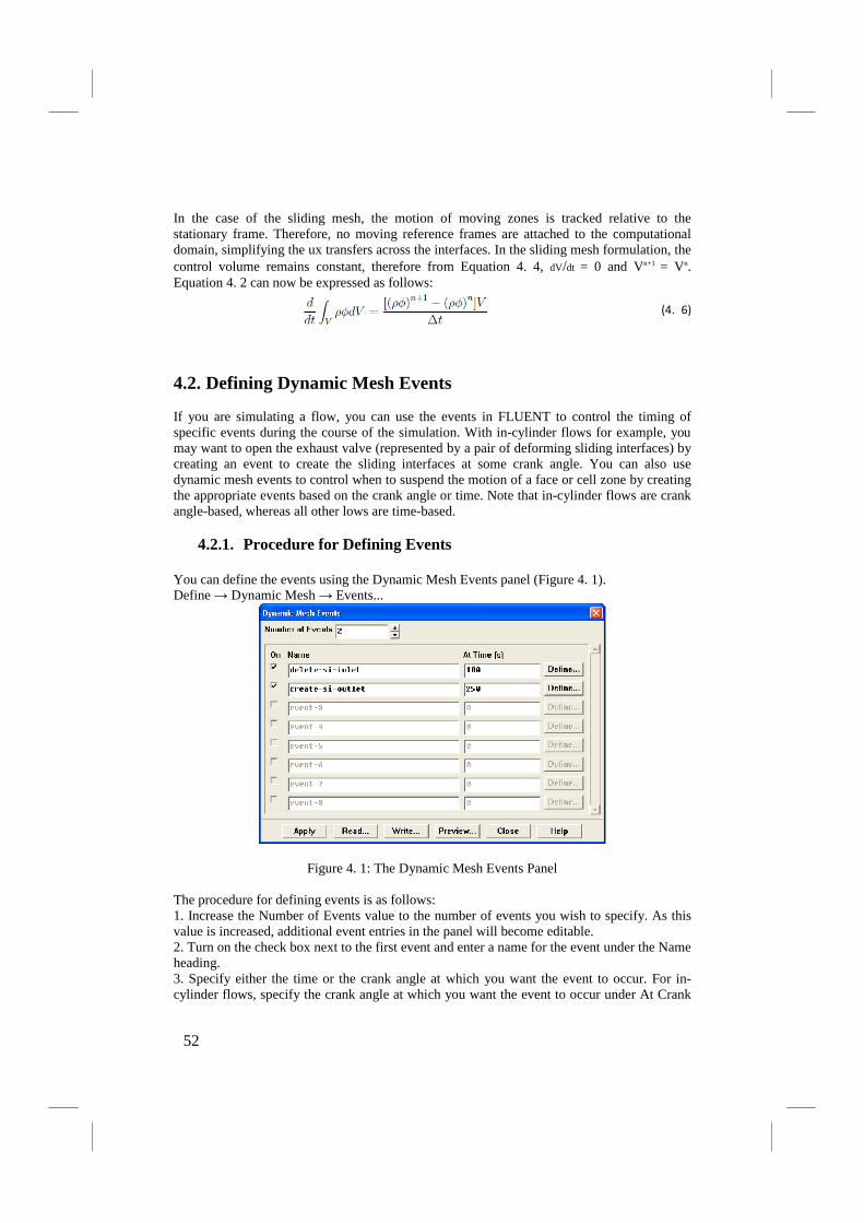
You can define the events using the Dynamic Mesh Events panel (Figure 4. 1). Define → Dynamic Mesh → Events...
Figure 4. 1: The Dynamic Mesh Events Panel
The procedure for defining events is as follows: 1. Increase the Number of Events value to the number of events you wish to specify. As this value is increased, additional event entries in the panel will become editable. 2. Turn on the check box next to the first event and enter a name for the event under the Name heading. 3. Specify either the time or the crank angle at which you want the event to occur. For in-cylinder flows, specify the crank angle at which you want the event to occur under At Crank
52
Angle. For non-in-cylinder flows, specify the time (in seconds) at which you want the event to occur under At Time.
It is not necessary to specify the events in order of increasing time or crank angle, but it may be easier to keep track of events if you specify them in the order of increasing time or angle.
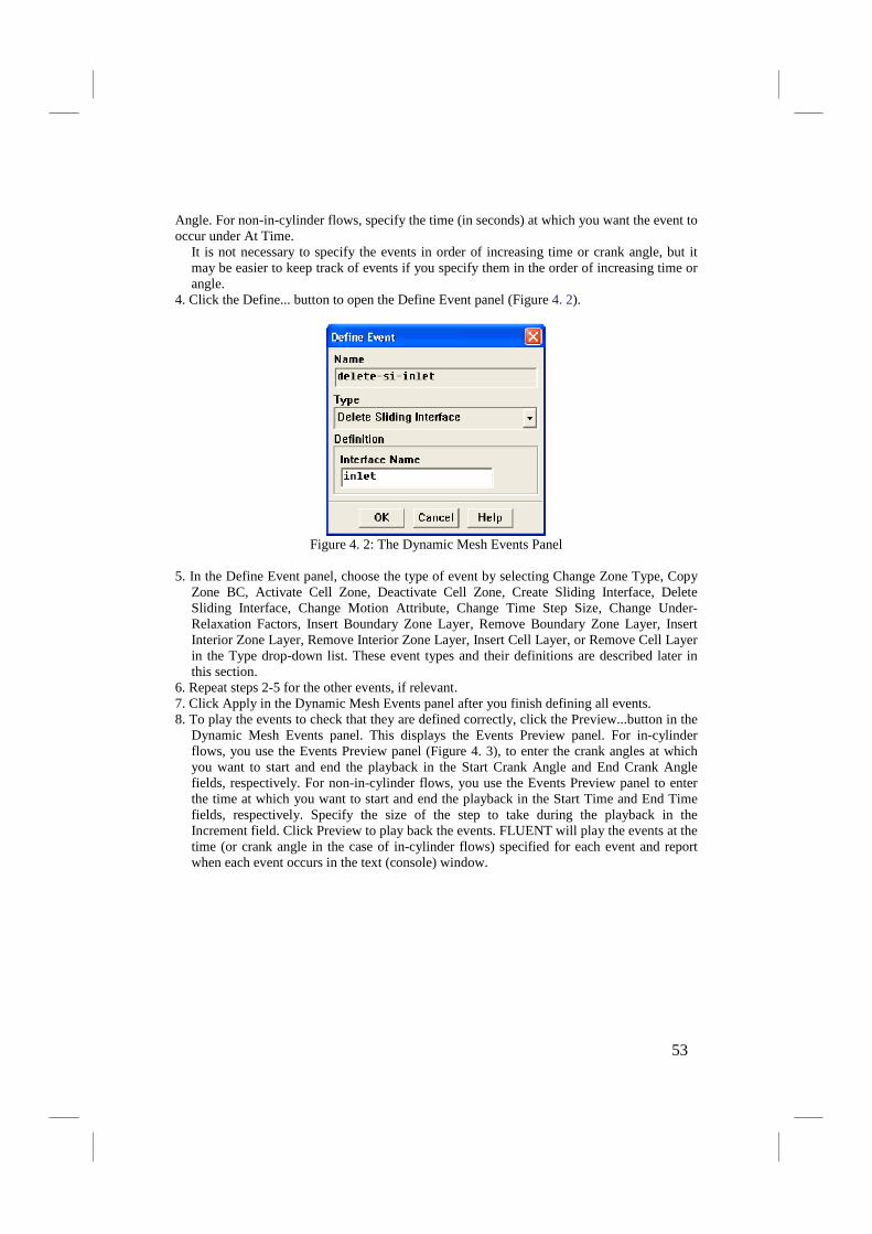
4. Click the Define... button to open the Define Event panel (Figure 4. 2).
Figure 4. 2: The Dynamic Mesh Events Panel
5. In the Define Event panel, choose the type of event by selecting Change Zone Type, Copy
Zone BC, Activate Cell Zone, Deactivate Cell Zone, Create Sliding Interface, Delete Sliding Interface, Change Motion Attribute, Change Time Step Size, Change Under-Relaxation Factors, Insert Boundary Zone Layer, Remove Boundary Zone Layer, Insert Interior Zone Layer, Remove Interior Zone Layer, Insert Cell Layer, or Remove Cell Layer in the Type drop-down list. These event types and their definitions are described later in this section.
6. Repeat steps 2-5 for the other events, if relevant. 7. Click Apply in the Dynamic Mesh Events panel after you finish defining all events. 8. To play the events to check that they are defined correctly, click the Preview...button in the
Dynamic Mesh Events panel. This displays the Events Preview panel. For in-cylinder flows, you use the Events Preview panel (Figure 4. 3), to enter the crank angles at which you want to start and end the playback in the Start Crank Angle and End Crank Angle fields, respectively. For non-in-cylinder flows, you use the Events Preview panel to enter the time at which you want to start and end the playback in the Start Time and End Time fields, respectively. Specify the size of the step to take during the playback in the Increment field. Click Preview to play back the events. FLUENT will play the events at the time (or crank angle in the case of in-cylinder flows) specified for each event and report when each event occurs in the text (console) window.
53

Figure 4. 3: The Events Preview Panel for In-Cylinder Flows
For in-cylinder simulations, you need to specify the events for one complete engine cycle. In the subsequent cycles, the events are executed whenever
(4. 7)
where θevent is the event crank angle, θc is the current crank angle, θperiod is the crank angle period for one cycle, and n is some integer. As an example, for in-cylinder simulations, you are not required to specify the event crank angle. FLUENT will execute an event if the current crank angle is between ±0:5 ∆θ where ∆θ is the equivalent change in crank angle for the time step. For example, if the event preview is executed between crank angle of 340° and 1060° (crank period is 720°) using an increment of 1°. Events Each of the available events is described below. Changing the Zone Type You can change the type of a zone to be a wall, or an interface, interior, uid, or solid zone during your simulation. To change the type of a zone, select Change Zone Type in the Type drop-down list in the Define Event panel (Figure 4. 2). Select the zone(s) that you want to change in the Zone(s) list, and then select the new zone type in the New Zone Type drop-down list. Copying Zone Boundary Conditions You can copy boundary conditions from one zone to other zones during your simulation. If, for example, you have changed an inlet zone to type wall with the Change Zone Type event, you can set the boundary conditions of the new zone type by simply copying the boundary conditions from a known zone with the corresponding zone type. To copy boundary conditions from one zone to another, select Copy Zone BC in the Type drop-down list in the Define Event panel (Figure 4. 2). In the From Zone drop-down list, select the zone that has the conditions you want to copy. In the To Zone(s) list, select the zone or zones to which you want to copy the conditions. FLUENT will set all of the boundary conditions for the zones selected in the To Zone(s) list to be the same as the conditions for the zone selected in the From Zone list. (You cannot copy a subset of the conditions, such as only the thermal conditions.) Note that you cannot copy conditions from external walls to internal (i.e., two-sided) walls, or vice versa, if the energy equation is being solved, since the thermal conditions for external and internal walls are different. Deactivating a Cell Zone To deactivate a cell zone, select Deactivate Cell Zone in the Type drop-down list in the Define Event panel (Figure 4. 2), then select the zone that you want to deactivate in the Zone(s) list. Only deactivated zones can be activated. When a zone is deactivated, FLUENT skips the zone during the calculations.
54
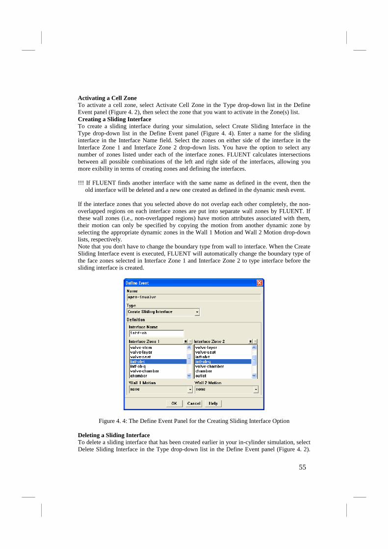
Activating a Cell Zone To activate a cell zone, select Activate Cell Zone in the Type drop-down list in the Define Event panel (Figure 4. 2), then select the zone that you want to activate in the Zone(s) list. Creating a Sliding Interface To create a sliding interface during your simulation, select Create Sliding Interface in the Type drop-down list in the Define Event panel (Figure 4. 4). Enter a name for the sliding interface in the Interface Name field. Select the zones on either side of the interface in the Interface Zone 1 and Interface Zone 2 drop-down lists. You have the option to select any number of zones listed under each of the interface zones. FLUENT calculates intersections between all possible combinations of the left and right side of the interfaces, allowing you more exibility in terms of creating zones and defining the interfaces. !!! If FLUENT finds another interface with the same name as defined in the event, then the
old interface will be deleted and a new one created as defined in the dynamic mesh event. If the interface zones that you selected above do not overlap each other completely, the non-overlapped regions on each interface zones are put into separate wall zones by FLUENT. If these wall zones (i.e., non-overlapped regions) have motion attributes associated with them, their motion can only be specified by copying the motion from another dynamic zone by selecting the appropriate dynamic zones in the Wall 1 Motion and Wall 2 Motion drop-down lists, respectively. Note that you don't have to change the boundary type from wall to interface. When the Create Sliding Interface event is executed, FLUENT will automatically change the boundary type of the face zones selected in Interface Zone 1 and Interface Zone 2 to type interface before the sliding interface is created.
Figure 4. 4: The Define Event Panel for the Creating Sliding Interface Option
Deleting a Sliding Interface To delete a sliding interface that has been created earlier in your in-cylinder simulation, select Delete Sliding Interface in the Type drop-down list in the Define Event panel (Figure 4. 2).
55
Enter the name of the sliding interface to be deleted in the Interface Name field. As with the Create Sliding Interface event, FLUENT will automatically change the corresponding interface zones to wall. However, you may want to use the Copy Zone BC event to set any boundary conditions that are not the default conditions that FLUENT assumes. Changing the Motion Attribute of a Dynamic Zone To change the motion attribute of a dynamic zone during your in-cylinder calculation, select Change Motion Attribute in the Type drop-down list in the Define Event panel (Figure 4. 2). Select the Attribute (slide, moving, or remesh) and set the appropriate Status (enable or disable). Select the corresponding dynamic zones for which you want to change the motion attributes in the Dynamic Zones list. The slide attribute is used to enable or disable smoothing of nodes on selected deforming face zones, the moving attribute is used to suspend the motion of selected moving zones, and the remesh attribute is used to enable and disable face remeshing on selected deforming face zones. Changing the Time Step To change the time step at some point during the simulation, select Change Time Step Size in the Type drop-down list in the Define Event panel. Specify the new physical time step size by entering the new Time Step Size in seconds. For in-cylinder simulations, specify the new physical time step by entering the new Crank Angle Step Size value in degrees. The physical time step is calculated from
(4. 8)
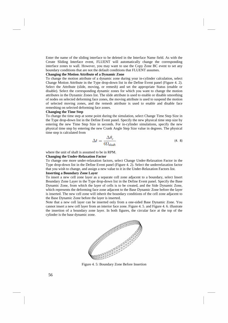
where the unit of shaft is assumed to be in RPM. Changing the Under-Relaxation Factor To change one more under-relaxation factors, select Change Under-Relaxation Factor in the Type drop-down list in the Define Event panel (Figure 4. 2). Select the underrelaxation factor that you wish to change, and assign a new value to it in the Under-Relaxation Factors list. Inserting a Boundary Zone Layer To insert a new cell zone layer as a separate cell zone adjacent to a boundary, select Insert Boundary Zone Layer in the Type drop-down list in the Define Event panel. Specify the Base Dynamic Zone, from which the layer of cells is to be created, and the Side Dynamic Zone, which represents the deforming face zone adjacent to the Base Dynamic Zone before the layer is inserted. The new cell zone will inherit the boundary conditions of the cell zone adjacent to the Base Dynamic Zone before the layer is inserted. Note that a new cell layer can be inserted only from a one-sided Base Dynamic Zone. You cannot insert a new cell layer from an interior face zone. Figure 4. 5. and Figure 4. 6. illustrate the insertion of a boundary zone layer. In both figures, the circular face at the top of the cylinder is the base dynamic zone.
Figure 4. 5: Boundary Zone Before Insertion
56

Figure 4. 6: Boundary Zone After Insertion
Removing a Boundary Zone Layer To remove the cell zone layer inserted using the Insert Boundary Zone Layer event, select Remove Boundary Zone Layer in the Type drop-down list in the Define Event panel. Specify the same Base Dynamic Zone that you used when you defined the insert boundary layer event. Note that a cell layer can be removed only from a one-sided Base Dynamic Zone. Inserting an Interior Zone Layer To insert a new zone layer as a separate cell zone adjacent to the internal side of a boundary, select Insert Interior Zone Layer in the Type drop-down list in the Define Event panel. Specify the Base Dynamic Zone and the Side Dynamic Zone as described in the Insert Boundary Zone Layer event. You also need to specify the names of the new interior face zones (Internal Zone 1 Name and Internal Zone 2 Name) that will be created after the cell zone layer is created by FLUENT. FLUENT inserts the interior cell layer by splitting the cell zone adjacent to the Base Dynamic Zone with a plane. The position of the plane and the normal direction of the plane are implicitly defined by the cylinder origin and cylinder axis of the Side Dynamic Zone.
Figure 4. 7: Boundary Zone After Insertion
Figure 4. 6 and Figure 4. 7 illustrate the insertion of an interior zone layer.
57
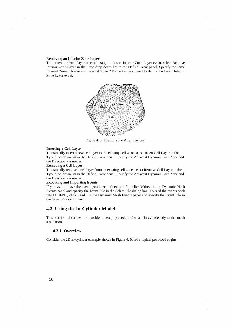
Removing an Interior Zone Layer To remove the zone layer inserted using the Insert Interior Zone Layer event, select Remove Interior Zone Layer in the Type drop-down list in the Define Event panel. Specify the same Internal Zone 1 Name and Internal Zone 2 Name that you used to define the Insert Interior Zone Layer event.
Figure 4. 8: Interior Zone After Insertion
Inserting a Cell Layer To manually insert a new cell layer to the existing cell zone, select Insert Cell Layer in the Type drop-down list in the Define Event panel. Specify the Adjacent Dynamic Face Zone and the Direction Parameter. Removing a Cell Layer To manually remove a cell layer from an existing cell zone, select Remove Cell Layer in the Type drop-down list in the Define Event panel. Specify the Adjacent Dynamic Face Zone and the Direction Parameter. Exporting and Importing Events If you want to save the events you have defined to a file, click Write... in the Dynamic Mesh Events panel and specify the Event File in the Select File dialog box. To read the events back into FLUENT, click Read... in the Dynamic Mesh Events panel and specify the Event File in the Select File dialog box. 4.3. Using the In-Cylinder Model This section describes the problem setup procedure for an in-cylinder dynamic mesh simulation.
4.3.1. Overview Consider the 2D in-cylinder example shown in Figure 4. 9. for a typical pent-roof engine.
58

Figure 4. 9: A 2D In-Cylinder Geometry
In setting up the dynamic mesh model for an in-cylinder problem, you need to consider the following issues:
• how to provide the proper mesh topology for the volume mesh update methods • (spring-based smoothing, dynamic layering, and local remeshing) • how to define the motion attributes and geometry for the valve and piston surfaces • how to address the opening and closing of the intake and exhaust valves • how to specify the sequence of events that controls the in-cylinder simulation
Defining the Mesh Topology FLUENT requires that you provide an initial volume mesh with the appropriate mesh topology such that the various mesh update methods described in: Dynamic Mesh Update Methods can be used to automatically update the dynamic mesh. However, FLUENT does not require you to set up all in-cylinder problems using the same mesh topology. When you generate the mesh for your in-cylinder model (using GAMBIT or other mesh generation tools), you need to consider the various mesh regions that you can identify as moving, deforming, or stationary, and generate these mesh regions with the appropriate cell shape. The mesh topology for the example problem in Figure 4. 9 is shown in Figure 4. 10, and the corresponding volume mesh is shown in Figure 4. 11.
59

Figure 4. 10: Mesh Topology Showing the Various Mesh Regions
Because of the rectilinear motion of the moving surfaces, you can use dynamic layering zones to represent the mesh regions swept out by the moving surfaces. These regions are the regions above the top surfaces of the intake and exhaust valves and above the piston head surface, and must be meshed with quadrilateral or hexahedral cells (as required by the dynamic layering method).
Figure 4. 11: Mesh Associated With the Chosen Topology
60
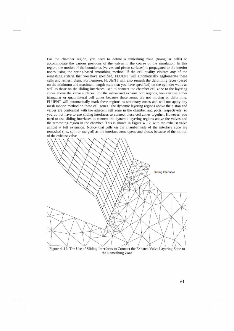
For the chamber region, you need to define a remeshing zone (triangular cells) to accommodate the various positions of the valves in the course of the simulation. In this region, the motion of the boundaries (valves and piston surfaces) is propagated to the interior nodes using the spring-based smoothing method. If the cell quality violates any of the remeshing criteria that you have specified, FLUENT will automatically agglomerate these cells and remesh them. Furthermore, FLUENT will also remesh the deforming faces (based on the minimum and maximum length scale that you have specified) on the cylinder walls as well as those on the sliding interfaces used to connect the chamber cell zone to the layering zones above the valve surfaces. For the intake and exhaust port regions, you can use either triangular or quadrilateral cell zones because these zones are not moving or deforming. FLUENT will automatically mark these regions as stationary zones and will not apply any mesh motion method on these cell zones. The dynamic layering regions above the piston and valves are conformal with the adjacent cell zone in the chamber and ports, respectively, so you do not have to use sliding interfaces to connect these cell zones together. However, you need to use sliding interfaces to connect the dynamic layering regions above the valves and the remeshing region in the chamber. This is shown in Figure 4. 12. with the exhaust valve almost at full extension. Notice that cells on the chamber side of the interface zone are remeshed (i.e., split or merged) as the interface zone opens and closes because of the motion of the exhaust valve.
Figure 4. 12: The Use of Sliding Interfaces to Connect the Exhaust Valve Layering Zone to
the Remeshing Zone
61
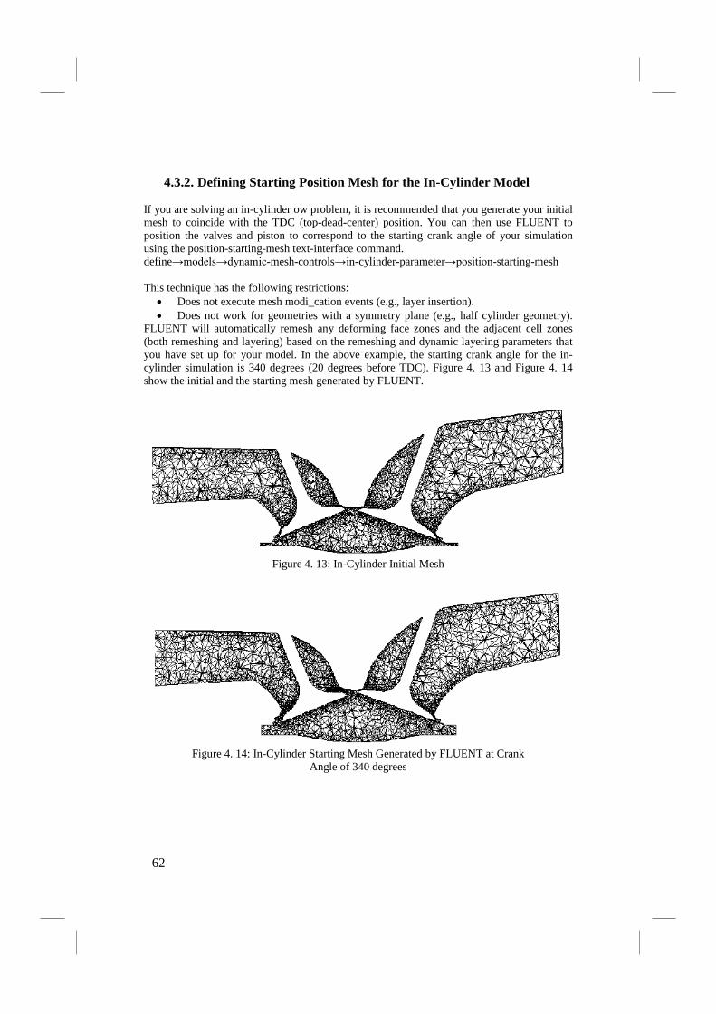
4.3.2. Defining Starting Position Mesh for the In-Cylinder Model If you are solving an in-cylinder ow problem, it is recommended that you generate your initial mesh to coincide with the TDC (top-dead-center) position. You can then use FLUENT to position the valves and piston to correspond to the starting crank angle of your simulation using the position-starting-mesh text-interface command. define→models→dynamic-mesh-controls→in-cylinder-parameter→position-starting-mesh This technique has the following restrictions:
• Does not execute mesh modi_cation events (e.g., layer insertion). • Does not work for geometries with a symmetry plane (e.g., half cylinder geometry).
FLUENT will automatically remesh any deforming face zones and the adjacent cell zones (both remeshing and layering) based on the remeshing and dynamic layering parameters that you have set up for your model. In the above example, the starting crank angle for the in-cylinder simulation is 340 degrees (20 degrees before TDC). Figure 4. 13 and Figure 4. 14 show the initial and the starting mesh generated by FLUENT.
Figure 4. 13: In-Cylinder Initial Mesh
Figure 4. 14: In-Cylinder Starting Mesh Generated by FLUENT at Crank
Angle of 340 degrees
62
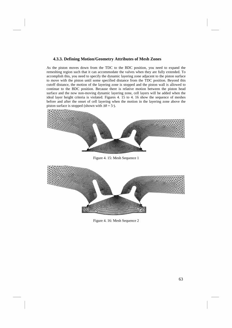
4.3.3. Defining Motion/Geometry Attributes of Mesh Zones As the piston moves down from the TDC to the BDC position, you need to expand the remeshing region such that it can accommodate the valves when they are fully extended. To accomplish this, you need to specify the dynamic layering zone adjacent to the piston surface to move with the piston until some specified distance from the TDC position. Beyond this cutoff distance, the motion of the layering zone is stopped and the piston wall is allowed to continue to the BDC position. Because there is relative motion between the piston head surface and the now non-moving dynamic layering zone, cell layers will be added when the ideal layer height criteria is violated. Figures 4. 15 to 4. 16 show the sequence of meshes before and after the onset of cell layering when the motion in the layering zone above the piston surface is stopped (shown with ∆θ = 5°).
Figure 4. 15: Mesh Sequence 1
Figure 4. 16: Mesh Sequence 2
63

Figure 4. 17: Mesh Sequence 3
Figure 4. 18: Mesh Sequence 4
64
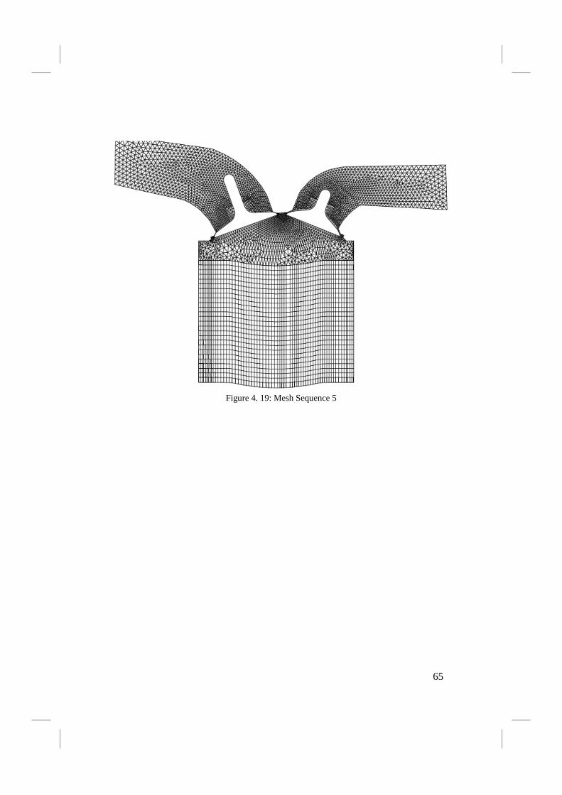
Figure 4. 19: Mesh Sequence 5
65
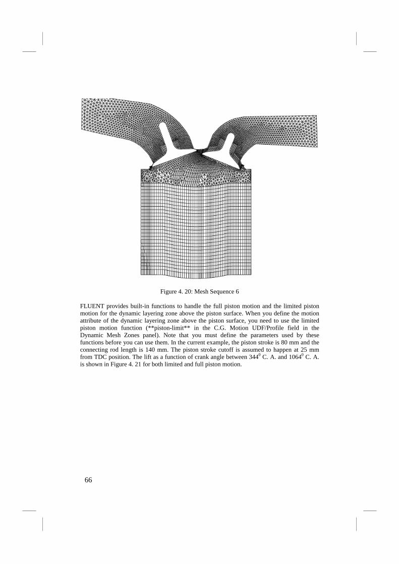
Figure 4. 20: Mesh Sequence 6
FLUENT provides built-in functions to handle the full piston motion and the limited piston motion for the dynamic layering zone above the piston surface. When you define the motion attribute of the dynamic layering zone above the piston surface, you need to use the limited piston motion function (**piston-limit** in the C.G. Motion UDF/Profile field in the Dynamic Mesh Zones panel). Note that you must define the parameters used by these functions before you can use them. In the current example, the piston stroke is 80 mm and the connecting rod length is 140 mm. The piston stroke cutoff is assumed to happen at 25 mm from TDC position. The lift as a function of crank angle between 3440 C. A. and 10640 C. A. is shown in Figure 4. 21 for both limited and full piston motion.
66

Figure 4. 21: Piston Position (m) as a Function of Crank Angle (deg)
To define the motion of the valves, you need to use profiles that describe the variation of valve lift with crank angle. FLUENT expects certain profile fields to be used to define the lift and the crank angle. FLUENT expects the angle and lift fields to define the crank angle and lift variations, respectively. The angle must be specified in degrees and the lift values must be in meters. The actual valve lift profiles that you will use for the current example are shown in Figure 4. 22. Notice that there is an overlapped period where both the intake and exhaust valves are open.
67
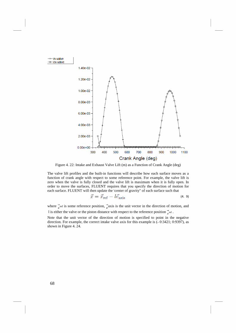
Figure 4. 22: Intake and Exhaust Valve Lift (m) as a Function of Crank Angle (deg)
The valve lift profiles and the built-in functions will describe how each surface moves as a function of crank angle with respect to some reference point. For example, the valve lift is zero when the valve is fully closed and the valve lift is maximum when it is fully open. In order to move the surfaces, FLUENT requires that you specify the direction of motion for each surface. FLUENT will then update the \center of gravity" of each surface such that
(4. 9)
where ref is some reference position, axis is the unit vector in the direction of motion, and l is either the valve or the piston distance with respect to the reference position ref . Note that the unit vector of the direction of motion is specified to point in the negative direction. For example, the correct intake valve axis for this example is (˗ 0:3421; 0:9397), as shown in Figure 4. 24.
68

Figure 4. 24: Definition of Valve Zone Attributes (Intake Valve)
4.3.4. Defining Valve Opening and Closure
FLUENT assumes that once you have set up the mesh topology, the mesh topology is unchanged throughout the entire simulation. Therefore, FLUENT does not allow you to completely close the valves such that the cells between the valve and the valve seat become degenerate (at cells) when these surfaces come in contact (removing these at cells would require the creation of new boundary face zones). To prevent the collapse, you need to define a minimum valve lift and FLUENT will automatically stop the motion of the valve when the valve lift is smaller than the minimum valve lift value. The minimum valve lift value can be specified in the Dynamic Mesh Parameters panel. For the current example, a minimum valve lift value of 0.1 mm is assumed. When the valve position is smaller than the minimum valve lift value, it is normal practice to assume that the valve is closed. The actual closing of the valves is accomplished by deleting the sliding interfaces that connect the chamber cell zone to the dynamic layering zones on the valves. The interface zones are then converted to walls to close off the \gaps" between the valves and the valve seats. The valve opening is achieved by the reverse process. When the valve lift has reached beyond the minimum valve lift value, the valve is assumed to be open and you can redefine the sliding interfaces such that the chamber zone is now connected to the dynamic layering zones above the valves.
4.3.5. Defining Events for In-Cylinder Applications FLUENT will automatically limit the valve lift values depending on the specified minimum valve lift value. However, the conversion of the sliding interface zones to walls (and vice versa) is accomplished via the in-cylinder events. For example, if the exhaust valve closes at -5° before TDC position, you must define a Delete Sliding Interface event at the crank angle of -5°. You need to define similar events for the intake valve opening (using the Create Sliding Interface event), the intake valve closing (Delete Sliding Interface event), and the exhaust valve opening (Create Sliding Interface event) at the respective crank angles. For the current example, the exhaust valve is assumed to be open between 131° and 371° and the intake valve is open between at 345° and 584°.
69
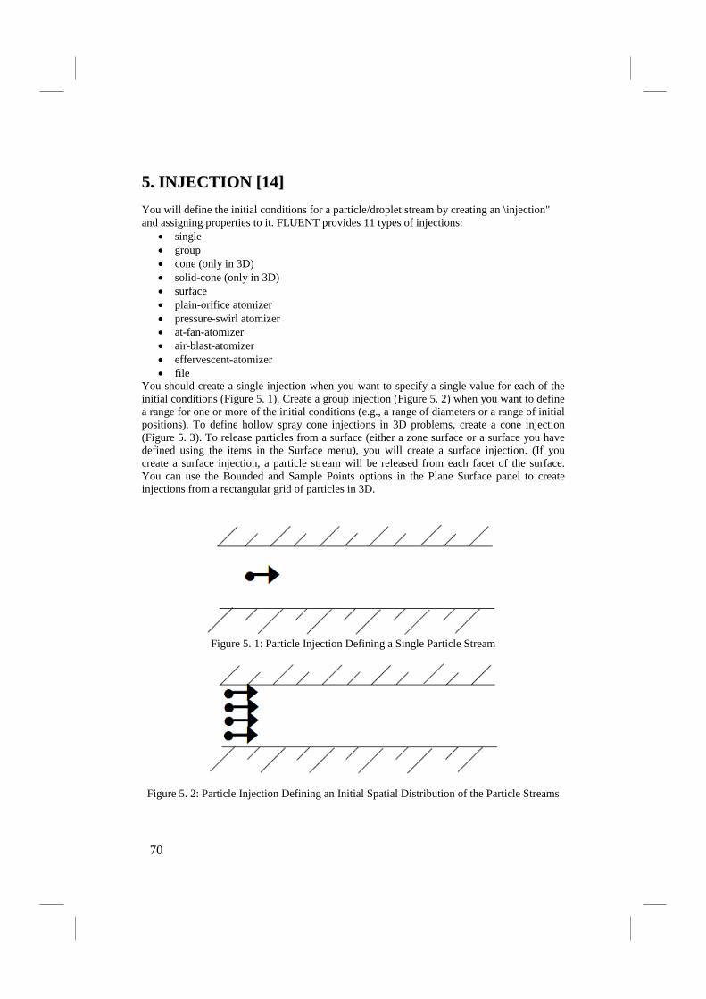
55.. IINNJJEECCTTIIOONN [[1144]] You will define the initial conditions for a particle/droplet stream by creating an \injection" and assigning properties to it. FLUENT provides 11 types of injections:
• single • group • cone (only in 3D) • solid-cone (only in 3D) • surface • plain-orifice atomizer • pressure-swirl atomizer • at-fan-atomizer • air-blast-atomizer • effervescent-atomizer • file
You should create a single injection when you want to specify a single value for each of the initial conditions (Figure 5. 1). Create a group injection (Figure 5. 2) when you want to define a range for one or more of the initial conditions (e.g., a range of diameters or a range of initial positions). To define hollow spray cone injections in 3D problems, create a cone injection (Figure 5. 3). To release particles from a surface (either a zone surface or a surface you have defined using the items in the Surface menu), you will create a surface injection. (If you create a surface injection, a particle stream will be released from each facet of the surface. You can use the Bounded and Sample Points options in the Plane Surface panel to create injections from a rectangular grid of particles in 3D.
Figure 5. 1: Particle Injection Defining a Single Particle Stream
Figure 5. 2: Particle Injection Defining an Initial Spatial Distribution of the Particle Streams
70

Figure 5. 3: Particle Injection Defining an Initial Spray Distribution of the Particle Velocity
Particle initial conditions (position, velocity, diameter, temperature, and mass flow rate) can also be read from an external file if none of the injection types listed above can be used to describe your injection distribution. The file has the following form: (( x y z u v w diameter temperature mass-flow) name ) with all of the parameters in SI units. All the parentheses are required, but the name is optional. 5.1. Point Properties for Single Injections For a single injection, you will define the following initial conditions for the particle stream under the Point Properties heading (in the Set Injection Properties panel):
• position Set the x, y, and z positions of the injected stream along the Cartesian axes of the problem geometry in the X-, Y-, and Z-Position fields. (Z-Position will appear only for 3D problems.)
• velocity Set the x, y, and z components of the stream's initial velocity in the X-, Y-, and Z-Velocity fields. (Z-Velocity will appear only for 3D problems.)
• diameter Set the initial diameter of the injected particle stream in the Diameter field.
• temperature Set the initial (absolute) temperature of the injected particle stream in the Temperature field.
• mass flow rate For coupled phase calculations, set the mass of particles per unit time that follows the trajectory defined by the injection in the Flow Rate field. Note that in axisymmetric problems the mass flow rate is defined per 2π radians and in 2D problems per unit meter depth (regardless of the reference value for length).
• duration of injection For unsteady particle tracking, set the starting and ending time for the injection in the Start Time and Stop Time fields.
5.2. Point Properties for Group Injections For group injections, you will define the properties described for single injections for the First Point and Last Point in the group. That is, you will define a range of values, ϕ1 through ϕN ,
71

for each initial condition ϕ by setting values for ϕ1 and ϕN. FLUENT assigns a value of ϕ to the ith injection in the group using a linear variation between the first and last values for ϕ:
(5. 1)
Thus, for example, if your group consists of 5 particle streams and you define a range for the initial x location from 0.2 to 0.6 meters, the initial x location of each stream is as follows:
• Stream 1: x = 0.2 meters • Stream 2: x = 0.3 meters • Stream 3: x = 0.4 meters • Stream 4: x = 0.5 meters • Stream 5: x = 0.6 meters
!!! In general, you should supply a range for only one of the initial conditions in a given group-leaving all other conditions fixed while a single condition varies among the stream numbers of the group. Otherwise you may find, for example, that your simultaneous inputs of a spatial distribution and a size distribution have placed the small droplets at the beginning of the spatial range and the large droplets at the end of the spatial range.
Note that you can use a different method for defining the size distribution of the particles, as discussed below. Using the Rosin-Rammler Diameter Distribution Method By default, you will define the size distribution of particles by inputting a diameter for the first and last points and using the linear equation to vary the diameter of each particle stream in the group. When you want a different mass flow rate for each particle/droplet size, however, the linear variation may not yield the distribution you need. Your particle size distribution may be defined most easily by fitting the size distribution data to the Rosin-Rammler equation. In this approach, the complete range of particle sizes is divided into a set of discrete size ranges, each to be defined by a single stream that is part of the group. Assume, for example, that the particle size data obeys the following distribution:
The Rosin-Rammler distribution function is based on the assumption that an exponential relationship exists between the droplet diameter, d, and the mass fraction of droplets with diameter greater than d, Yd:
(5. 2)
FLUENT refers to the quantity d in Equation 4. 1 as the Mean Diameter and to n as the Spread Parameter. These parameters are input by you (in the Set Injection Properties panel under the First Point heading) to define the Rosin-Rammler size distribution. To solve for these parameters, you must fit your particle size data to the Rosin-Rammler exponential
72
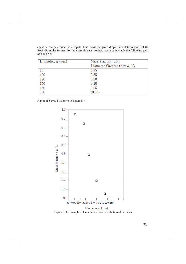
equation. To determine these inputs, first recast the given droplet size data in terms of the Rosin-Rammler format. For the example data provided above, this yields the following pairs of d and Yd:
A plot of Yd vs. d is shown in Figure 5. 4.
Figure 5. 4: Example of Cumulative Size Distribution of Particles
73
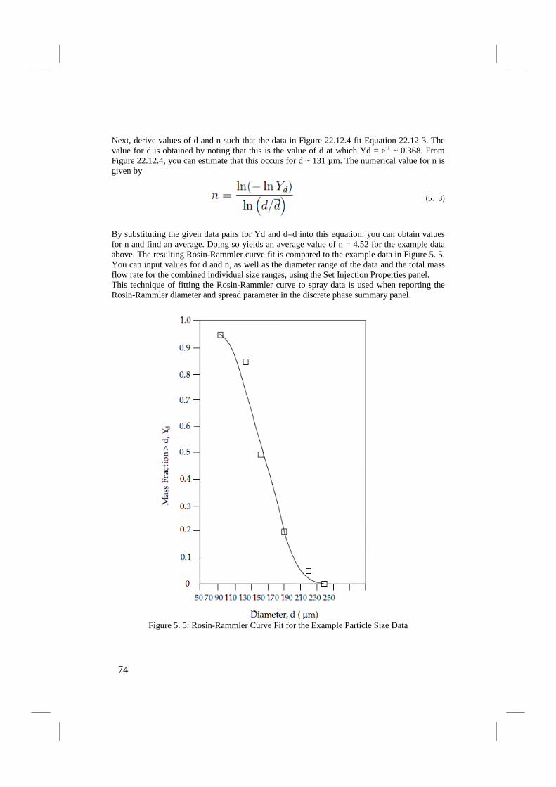
Next, derive values of d and n such that the data in Figure 22.12.4 fit Equation 22.12-3. The value for d is obtained by noting that this is the value of d at which Yd = e-1 ~ 0.368. From Figure 22.12.4, you can estimate that this occurs for d ~ 131 µm. The numerical value for n is given by
(5. 3)
By substituting the given data pairs for Yd and d=d into this equation, you can obtain values for n and find an average. Doing so yields an average value of n = 4.52 for the example data above. The resulting Rosin-Rammler curve fit is compared to the example data in Figure 5. 5. You can input values for d and n, as well as the diameter range of the data and the total mass flow rate for the combined individual size ranges, using the Set Injection Properties panel. This technique of fitting the Rosin-Rammler curve to spray data is used when reporting the Rosin-Rammler diameter and spread parameter in the discrete phase summary panel.
Figure 5. 5: Rosin-Rammler Curve Fit for the Example Particle Size Data
74
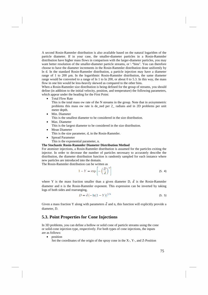
A second Rosin-Rammler distribution is also available based on the natural logarithm of the particle diameter. If in your case, the smaller-diameter particles in a Rosin-Rammler distribution have higher mass flows in comparison with the larger-diameter particles, you may want better resolution of the smaller-diameter particle streams, or \ “bins". You can therefore choose to have the diameter increments in the Rosin-Rammler distribution done uniformly by ln d. In the standard Rosin-Rammler distribution, a particle injection may have a diameter range of 1 to 200 µm. In the logarithmic Rosin-Rammler distribution, the same diameter range would be converted to a range of ln 1 to ln 200, or about 0 to 5.3. In this way, the mass flow in one bin would be less-heavily skewed as compared to the other bins. When a Rosin-Rammler size distribution is being defined for the group of streams, you should define (in addition to the initial velocity, position, and temperature) the following parameters, which appear under the heading for the First Point:
• Total Flow Rate This is the total mass ow rate of the N streams in the group. Note that in axisymmetric problems this mass ow rate is de_ned per 2_ radians and in 2D problems per unit meter depth.
• Min. Diameter This is the smallest diameter to be considered in the size distribution.
• Max. Diameter This is the largest diameter to be considered in the size distribution.
• Mean Diameter This is the size parameter, d, in the Rosin-Rammler.
• Spread Parameter This is the exponential parameter, n.
The Stochastic Rosin-Rammler Diameter Distribution Method For atomizer injections, a Rosin-Rammler distribution is assumed for the particles exiting the injector. In order to decrease the number of particles necessary to accurately describe the distribution, the diameter distribution function is randomly sampled for each instance where new particles are introduced into the domain. The Rosin-Rammler distribution can be written as
(5. 4)
where Y is the mass fraction smaller than a given diameter D, is the Rosin-Rammler diameter and n is the Rosin-Rammler exponent. This expression can be inverted by taking logs of both sides and rearranging,
(5. 5)
Given a mass fraction Y along with parameters and n, this function will explicitly provide a diameter, D. 5.3. Point Properties for Cone Injections In 3D problems, you can define a hollow or solid cone of particle streams using the cone or solid-cone injection type, respectively. For both types of cone injections, the inputs are as follows:
• position Set the coordinates of the origin of the spray cone in the X-, Y-, and Z-Position
75
• fields. • diameter
Set the diameter of the particles in the stream in the Diameter field. • temperature
Set the temperature of the streams in the Temperature field. • axis
Set the x, y, and z components of the vector defining the cone's axis in the X-Axis, Y-Axis, and Z-Axis fields.
• velocity Set the velocity magnitude of the particle streams that will be oriented along the specified spray cone angle in the Velocity Mag. field.
• cone angle Set the included half-angle, _, of the hollow spray cone in the Cone Angle field, as show in Figure 5. 6.
Figure 5. 6: Cone Half Angle and Radius
• radius
A nonzero inner radius can be specified to model injectors that do not emanate from a single point. Set the radius r (defined as shown in Figure 5. 6) in the Radius field. The particles will be distributed about the axis with the specified radius.
• swirl fraction (hollow cone only) Set the fraction of the velocity magnitude to go into the swirling component of the flow in the Swirl Fraction field. The direction of the swirl component is defined using the right-hand rule about the axis (a negative value for the swirl fraction can be used to reverse the swirl direction).
• mass flow rate For coupled calculations, set the total mass flow rate for the streams in the spray cone in the Total Flow Rate field.
The distribution of the particle streams for the solid cone injection is random, as seen in Figure 5. 3. Furthermore, duplicating this injection may not necessarily result in the same distribution, at the same location.
76
For transient calculations, the spatial distribution of streams at the initial injection location is recalculated at each time step. Sampling different possible trajectories allows a more accurate representation of a solid cone using fewer computational parcels. For steady state calculations, the trajectories are initialized one time and kept the same for subsequent DPM iterations. The trajectories are recalculated when a change in the injection panel occurs or when a case and data file are saved. If the residuals and solution change when a small change is made to the injection or when a case and data file are saved, it may mean that there are not enough trajectories being used to represent the solid cone with sufficient accuracy. Note that you may want to define multiple spray cones emanating from the same initial location in order to specify a size known distribution of the spray or to include a known range of cone angles. 5.4. Point Properties for Surface Injections For surface injections, you will define all the properties described in Section Point Properties for Single Injections for single injections except for the initial position of the particle streams. The initial positions of the particles will be the location of the data points on the specified surface(s). Note that you will set the Total Flow Rate of all particles released from the surface (required for coupled calculations only). If you want, you can scale the individual mass flow rates of the particles by the ratio of the area of the face they are released from to the total area of the surface. To scale the mass flow rates, select the Scale Flow Rate By Face Area option under Point Properties. Note that many surfaces have nonuniform distributions of points. If you want to generate a uniform spatial distribution of particle streams released from a surface in 3D, you can create a bounded plane surface with a uniform distribution using the Plane Surface panel, as described in Section Plane Surfaces. In 2D, you can create a rake using the Line/Rake Surface panel, as described in Section Line and Rake Surfaces. In addition to the option of scaling the ow rate by the face area, the normal direction of a face can be used for the injection direction. To use the face normal direction for the injection direction, select the Inject Using Normal Direction option under Point Properties. Once this option is selected, you only need to specify the velocity magnitude of the injection, not the individual components of the velocity magnitude. Note also that only surface injections from boundary surfaces will be moved with the grid when a sliding mesh or a moving or deforming mesh is being used. A nonuniform size distribution can be used for surface injections, as described below. Using the Rosin-Rammler Diameter Distribution Method The Rosin-Rammler size distributions described in Section Using the Rosin-Rammler Diameter Distribution Method for group injections is also available for surface injections. If you select one of the Rosin-Rammler distributions, you will need to specify the following parameters under Point Properties, in addition to the initial velocity, temperature, and total ow rate:
• Min. Diameter This is the smallest diameter to be considered in the size distribution.
• Max. Diameter This is the largest diameter to be considered in the size distribution.
• Mean Diameter This is the size parameter, d, in the Rosin-Rammler equation.
• Spread Parameter
77
This is the exponential parameter, n. • Number of Diameters
This is the number of diameters in each distribution (i.e., the number of different diameters in the stream injected from each face of the surface).
FLUENT will inject streams of particles from each face on the surface, with diameters defined by the Rosin-Rammler distribution function. The total number of injection streams tracked for the surface injection will be equal to the number of diameters in each distribution (Number of Diameters) multiplied by the number of faces on the surface. Point Properties for Plain-Orifice Atomizer Injections For a plain-orifice atomizer injection, you will define the following initial conditions under Point Properties:
• position Set the x, y, and z positions of the injected stream along the Cartesian axes of the problem geometry in the X-Position, Y-Position, and Z-Position fields. (Z-Position will appear only for 3D problems).
• axis (3D only) Set the x, y, and z components of the vector defining the axis of the orifice in the X-Axis, Y-Axis, and Z-Axis fields.
• temperature • Set the temperature of the streams in the Temperature field. • mass flow rate
Set the mass flow rate for the streams in the atomizer in the Flow Rate field. Note that in 3D sectors, the flow rate must be appropriate for the sector defined by the Azimuthal Start Angle and Azimuthal Stop Angle.
• duration of injection • For unsteady particle tracking, set the starting and ending time for the injection in the
Start Time and Stop Time fields. • vapor pressure Set the vapor pressure governing the flow through the internal orifice
in the Vapor Pressure field. • Diameter Set the diameter of the orifice in the Injector Inner Diam. field. • orifice length Set the length of the orifice in the Orifice Length field. • radius of curvature
Set the radius of curvature of the inlet corner in the Corner Radius of Curv. • nozzle parameter
Set the constant for the spray angle correlation in the Constant A field. • azimuthal angles
For 3D sectors, set the Azimuthal Start Angle and Azimuthal Stop Angle.
78
66.. MMOODDEELLIINNGG EENNGGIINNEE IIGGNNIITTIIOONN [[1144]] This chapter describes only the engine ignition for Autoignition Models due to the fact
that this course book comprises only deliberation of compression-ignition engine.
6.1. Autoignition Models Autoignition phenomena in engines are due to the effects of chemical kinetics of the reacting flow inside the cylinder. There are two types of autoignition models considered in FLUENT:
• knock model in spark-ignited (SI) engines • ignition delay model in diesel engines
Autoignition models in FLUENT are described in the following sections.
6.1.1. Overview The concept of knock has been studied extensively in the context of premixed engines, as it defines a limit in terms of efficiency and power production of that type of engine. As the compression ratio increases, the efficiency of the engine as a function of the work extracted from the fuel increases. However, as the compression ratio increases, the temperature and pressure of the air/fuel mixture in the cylinder also increase during the cycle compressions. The temperature and pressure increase can be large enough for the mixture to spontaneously ignite and release its heat before the spark plug fires. The premature release of all of the energy in the air/fuel charge is almost never desirable, as this results in the spark event no longer controlling the combustion. As a result of the premature release of the energy, catastrophic damage to the engine components can occur. The sudden, sharp rise in pressure inside the engine can be heard clearly through the engine block as a knocking sound, hence the term \knock". For commonly available gasoline pumps, knock usually limits the highest practical compression ratio to less than 11:1 for premium fuels and around 9:1 for less expensive fuels. By comparison, ignition delay in diesel engines has not been as extensively studied as SI engines, mainly because it does not have such a sharply defining impact on engine efficiency. Ignition delay in diesel engines refers to the time between when the fuel is injected into the combustion chamber and when the pressure starts to increase as the fuel releases its energy. The fuel is injected into a gas which is usually air, however, it can have a considerable amount of exhaust gas mixed in (or EGR) to reduce nitrogen oxide emissions (NOx). Ignition delay depends on the composition of the gas in the cylinder, the temperature of the gas, the turbulence level, and other factors. Since ignition delay changes the combustion phasing, which in turn impacts efficiency and emissions, it is important to account for it in a diesel engine simulation.
6.1.2. Model Limitations The main difference between the knock model and the ignition delay model is the manner in which the model is coupled with the chemistry. The knock model always releases energy from the fuel while the ignition delay model prevents energy from being released prematurely. The knock model in FLUENT is compatible with the premixed and partially premixed combustion models. The autoignition model is compatible with any volumetric combustion model, with the exception of the purely premixed models. The autoignition models are inherently transient and so are not available with steady simulations. The autoignition models in general require
79

adjustment of parameters to reproduce engine data and are likely to require tuning to improve accuracy. Once the model is calibrated to a particular engine configuration, then different engine speeds and loads can be reasonably well represented. Detailed chemical kinetics may be more applicable over a wider range of conditions, though are more expensive to solve. The single equation autoignition models are appropriate for the situation where geometric fidelity or resolution of particular flow details is more important than chemical effects on the simulation. 6.2. Ignition Model Theory Both the knock and the ignition delay models are treated similarly in FLUENT, in that they share the same infrastructure. These models belong to the family of single equation autoignition models and use correlations to account for complex chemical kinetics. They differ from the eight step reaction models, such as Halstead's \Shell" model [19], in that only a single transport equation is solved. The source term in the transport equation is typically not stiff, thus making the equation relatively inexpensive to solve. This approach is appropriate for large simulations where geometric accuracy is more important than fully resolved chemical kinetics. The model can be used on less resolved meshes to explore a range of designs quickly, and to obtain trends before utilizing more expensive and presumably more accurate chemical mechanisms in multidimensional simulations. 6.3. Transport of Ignition Species Autoignition is modeled using the transport equation for an Ignition Species, Yig, which is given by
(6. 1)
where Yig is a \mass fraction" of a passive species representing radicals which form when the fuel in the domain breaks down. Sct is the turbulent Schmidt number. The term Sig is the source term for the ignition species which has a form
(6. 2)
where t0 corresponds to the time at which fuel is introduced into the domain. The τig term is a correlation of ignition delay with the units of time. Ignition has occurred when the ignition species reaches a value of 1 in the domain. It is assumed that all the radical species represented by Yig diffuse at the same rate as the mean flow. Note that the source term for these radical species is treated differently for knock and ignition delay. Furthermore, the form of the correlation of ignition delay differs between the two models. Details of how the source term is treated are covered in the following sections. 6.4. Knock Modeling When modeling knock or ignition delay, chemical energy in the fuel is released when the ignition species reaches a value of 1 in the domain. For the knock model, two correlations are built into FLUENT. One is given by Douaud [10], while the other is a generalized model which reproduces several correlations, given by Heywood [20].
80
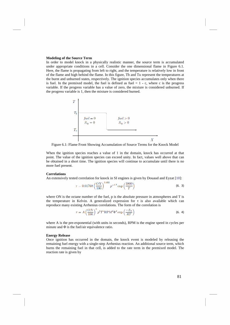
Modeling of the Source Term In order to model knock in a physically realistic manner, the source term is accumulated under appropriate conditions in a cell. Consider the one dimensional flame in Figure 6.1. Here, the flame is propagating from left to right, and the temperature is relatively low in front of the flame and high behind the flame. In this figure, Tb and Tu represent the temperatures at the burnt and unburned states, respectively. The ignition species accumulates only when there is fuel. In the premixed model, the fuel is defined as fuel = 1 ˗ c, where c is the progress variable. If the progress variable has a value of zero, the mixture is considered unburned. If the progress variable is 1, then the mixture is considered burned.
Figure 6.1: Flame Front Showing Accumulation of Source Terms for the Knock Model
When the ignition species reaches a value of 1 in the domain, knock has occurred at that point. The value of the ignition species can exceed unity. In fact, values well above that can be obtained in a short time. The ignition species will continue to accumulate until there is no more fuel present. Correlations An extensively tested correlation for knock in SI engines is given by Douaud and Eyzat [10]:
(6. 3)
where ON is the octane number of the fuel, p is the absolute pressure in atmospheres and T is the temperature in Kelvin. A generalized expression for τ is also available which can reproduce many existing Arrhenius correlations. The form of the correlation is
(6. 4)
where A is the pre-exponential (with units in seconds), RPM is the engine speed in cycles per minute and Φ is the fuel/air equivalence ratio. Energy Release Once ignition has occurred in the domain, the knock event is modeled by releasing the remaining fuel energy with a single-step Arrhenius reaction. An additional source term, which burns the remaining fuel in that cell, is added to the rate term in the premixed model. The reaction rate is given by
81

(6. 5)
where A0 = 8:6 x 10⁹, and Ea = -15078. These values are chosen to reect single-step reaction rates appropriate for propane as described in Amsden [3]. The rate at which the fuel is consumed is limited such that a completely unburned cell will burn during three of the current time steps. Limiting the reaction rate is done purely for numerical stability. 6.5. Ignition Delay Modeling When modeling ignition delay in diesel engines, chemical reactions are allowed to occur when the ignition species reaches a value of 1 in the domain. For the ignition delay model, two correlations are built into FLUENT, one given by Hardenburg and Hase [20] and the other, a generalized model which reproduces several Arrhenius correlations from the literature. If the ignition species is less than 1 when using the ignition delay model, the chemical source term is suppressed by not activating the combustion model at that particular time step; thus, the energy release is delayed. This approach is reasonable if the user has a good high-temperature chemical model, but does not wish to solve for typically expensive low temperature chemistry. 6.6. Modeling of the Source Term In order to model ignition in a physically realistic manner, the source term is accumulated under appropriate conditions in a cell. Consider the one dimensional spray in Figure 6.2. Here, the spray is propagating from left to right and the fuel mass fraction is
Figure 19.2.2: Propagating Fuel Cloud Showing Accumulation of Source Terms for the
Ignition Delay Model
relatively low in front of the spray and high behind the spray. If there is no fuel in the cell, the model will set the local source term to zero, nevertheless, the value of Yig can be nonzero due to convection and diffusion. 6.7. Correlations If fuel is present in the cell, there are two built-in options in FLUENT to calculate the local source term. The first correlation was done by Hardenburg and Hase and was developed at
82

Daimler Chrysler for heavy duty diesel engines. The correlation works over a reasonably wide range of conditions and is given by
(6. 6)
where fid is in seconds, C1 is 0.36, N is engine speed in revolutions per minute, Ea is the effective activation energy and ep is the pressure exponent. The expression for the effective activation energy is given by
(6. 7)
where CN is the cetane number. The activation energy, Ehh, pre-exponential, C1, pressure exponent, ep, and cetane number, CN, are accessible from the GUI. The default values of these variables are listed in the table below.
Table 6.1: Default Values of the Variables in the Hardenburg Correlation
The second correlation, which is the generalized correlation, and is available for ignition delay calculations. Energy Release If the ignition species is greater than or equal to 1 anywhere in the domain, ignition has occurred and combustion is no longer delayed. The ignition species acts as a switch to turn on the volumetric reactions in the domain. Note that the ignition species \mass fraction" can exceed 1 in the domain, therefore, it is not truly a mass fraction, but rather a passive scalar which represents the integrated correlation as a function of time. 6.8. Using the Autoignition Models To activate the autoignition model, perform the following steps: 1. Select Unsteady from the Time list in the Solver panel. 2. Select an appropriate reaction model in the Define/Models/Species submenu. Define → Models → Species → Transport & Reaction... 3. The models in the Species Model panel that are compatible with the autoignition model are Species Transport, Premixed Combustion, and Partially Premixed Combustion. !!! If you select Species Transport, you must also enable the Volumetric option in the Reactions group box. !!! The Premixed Combustion and Partially Premixed Combustion models are only available for turbulent lows using the pressure-based solver. 4. The Define/Models/Species submenu contains the Autoignition... model, which is now selectable. Select the Autoignition... model.
• If Species Transport is selected in the Species Model panel, you can only select the Ignition Delay Model.
83

Figure 6.3: The Ignition Delay Model in the Autoignition Model Panel
• If Premixed Combustion is selected in the Species Model panel, you can only select
the Knock Model.
Figure 6.4: The Knock Model in the Autoignition Model Panel
• If Partially Premixed Combustion is selected in the Species Model panel, you can select either the Knock Model or the Ignition Delay Model.
5. When the Ignition Delay Model is enabled, the panel expands to include the modeling parameters for this model (Figure 6.5). The two correlation options that exist with this model are the Hardenburg and the Generalized. Depending on which correlation option is selected, the appropriate modeling parameters will appear in the panel.
Figure 6.5: The Ignition Delay Model for the Partially Premixed Combustion Model
84
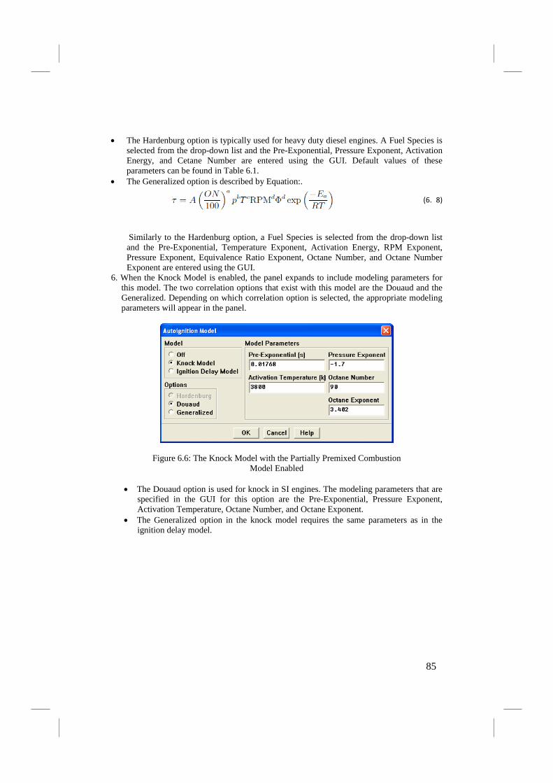
• The Hardenburg option is typically used for heavy duty diesel engines. A Fuel Species is selected from the drop-down list and the Pre-Exponential, Pressure Exponent, Activation Energy, and Cetane Number are entered using the GUI. Default values of these parameters can be found in Table 6.1.
• The Generalized option is described by Equation:.
(6. 8)
Similarly to the Hardenburg option, a Fuel Species is selected from the drop-down list and the Pre-Exponential, Temperature Exponent, Activation Energy, RPM Exponent, Pressure Exponent, Equivalence Ratio Exponent, Octane Number, and Octane Number Exponent are entered using the GUI.
6. When the Knock Model is enabled, the panel expands to include modeling parameters for this model. The two correlation options that exist with this model are the Douaud and the Generalized. Depending on which correlation option is selected, the appropriate modeling parameters will appear in the panel.
Figure 6.6: The Knock Model with the Partially Premixed Combustion Model Enabled
• The Douaud option is used for knock in SI engines. The modeling parameters that are
specified in the GUI for this option are the Pre-Exponential, Pressure Exponent, Activation Temperature, Octane Number, and Octane Exponent.
• The Generalized option in the knock model requires the same parameters as in the ignition delay model.
85
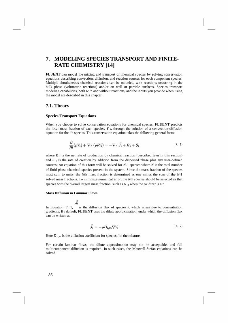
77.. MMOODDEELLIINNGG SSPPEECCIIEESS TTRRAANNSSPPOORRTT AANNDD FFIINNIITTEE--RRAATTEE CCHHEEMMIISSTTRRYY [[1144]]
FLUENT can model the mixing and transport of chemical species by solving conservation equations describing convection, diffusion, and reaction sources for each component species. Multiple simultaneous chemical reactions can be modeled, with reactions occurring in the bulk phase (volumetric reactions) and/or on wall or particle surfaces. Species transport modeling capabilities, both with and without reactions, and the inputs you provide when using the model are described in this chapter.
7.1. Theory
Species Transport Equations
When you choose to solve conservation equations for chemical species, FLUENT predicts the local mass fraction of each species, Y
i, through the solution of a convection-diffusion equation for the ith species. This conservation equation takes the following general form:
(7. 1)
where R i is the net rate of production by chemical reaction (described later in this section) and S i is the rate of creation by addition from the dispersed phase plus any user-defined sources. An equation of this form will be solved for N-1 species where N is the total number of fluid phase chemical species present in the system. Since the mass fraction of the species must sum to unity, the Nth mass fraction is determined as one minus the sum of the N-1 solved mass fractions. To minimize numerical error, the Nth species should be selected as that species with the overall largest mass fraction, such as N 2
Mass Diffusion in Laminar Flows
when the oxidizer is air.
In Equation 7. 1, is the diffusion flux of species i, which arises due to concentration gradients. By default, FLUENT uses the dilute approximation, under which the diffusion flux can be written as
(7. 2)
Here D i, m
For certain laminar flows, the dilute approximation may not be acceptable, and full multicomponent diffusion is required. In such cases, the Maxwell-Stefan equations can be solved.
is the diffusion coefficient for species i in the mixture.
86

Mass Diffusion in Turbulent Flows
In turbulent flows, FLUENT computes the mass diffusion in the following form:
(7. 3)
where is the turbulent Schmidt number, (with a default setting of 0.7). Note that turbulent diffusion generally overwhelms laminar diffusion, and the specification of detailed laminar diffusion properties in turbulent flows is not warranted.
Treatment of Species Transport in the Energy Equation
For many multicomponent mixing flows, the transport of enthalpy due to species diffusion
can have a significant effect on the enthalpy field and should not be neglected. In particular, when the Lewis number
(7. 4)
for any species is far from unity, neglecting this term can lead to significant errors. FLUENT will include this term by default. In Equation 7. 4, k is the thermal conductivity.
Diffusion at Inlets
For the segregated solver in FLUENT, the net transport of species at inlets consists of both the convection and diffusion components. (For the coupled solvers, only the convection component is included.) The convection component is fixed by the inlet species concentration specified by you. The diffusion component, however, depends on the gradient of the computed species concentration field. Thus the diffusion component (and therefore the net inlet transport) is not specified a priori.
The Generalized Finite-Rate Formulation for Reaction Modeling
The reaction rates that appear as source terms are computed in FLUENT by one of three models:
• Laminar finite-rate model: The effect of turbulent fluctuations are ignored, and reaction rates are determined by Arrhenius expressions.
87

• Eddy-dissipation model: Reaction rates are assumed to be controlled by the turbulence, so expensive Arrhenius chemical kinetic calculations can be avioded.
• Eddy-dissipation-concept (EDC) model: Detailed Arrhenius chemical kinetics can be incorporated in turbulent flames. Note that detailed chemical kinetic calculations are computationally expensive.
The generalized finite-rate formulation is suitable for a wide range of applications including laminar or turbulent reaction systems, and combustion systems with premixed, non-premixed, or partially-premixed flames.
The Laminar Finite-Rate Model
The laminar finite-rate model computes the chemical source terms using Arrhenius expressions, and ignores the effects of turbulent fluctuations. The model is exact for laminar flames, but is generally inaccurate for turbulent flames due to highly non-linear Arrhenius chemical kinetics. The laminar model may, however, be acceptable for combustion with relatively slow chemistry and small turbulent fluctuations, such as supersonic flames.
The net source of chemical species i due to reaction R i is computed as the sum of the Arrhenius reaction sources over the N R
reactions that the species participate in:
(7. 5)
where M w, i is the molecular weight of species i and is the Arrhenius molar rate of creation/destruction of species i in reaction r. Reaction may occur in the continuous phase between continuous-phase species only, or at wall surfaces resulting in the surface deposition or evolution of a continuous-phase species.
Consider the rth reaction written in general form as follows:
(7. 6)
88

where
N = number of chemical species in the system
= stoichiometric coefficient for reactant i in reaction r
= stoichiometric coefficient for product i in reaction r
= symbol denoting species i
k = f, r forward rate constant for reaction r
k = b, r backward rate constant for reaction r
Equation 7. 6 is valid for both reversible and non-reversible reactions. (Reactions in FLUENT are non-reversible by default.) For non-reversible reactions, the backward rate constant, k b, r
The summations in Equation 7. 6 are for all chemical species in the system, but only species that appear as reactants or products will have non-zero stoichiometric coefficients. Hence, species that are not involved will drop out of the equation.
, is simply omitted.
The molar rate of creation/destruction of species i in reaction r ( in Equation 7. 5) is given by
(7. 7)
where
N = r number of chemical species in reaction r
C = j, r molar concentration of each reactant and product
species j in reaction r (kgmol/m 3)
89
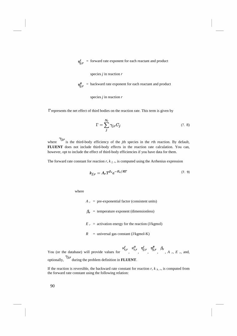
= forward rate exponent for each reactant and product
species j in reaction r
= backward rate exponent for each reactant and product
species j in reaction r
represents the net effect of third bodies on the reaction rate. This term is given by
(7. 8)
where is the third-body efficiency of the jth species in the rth reaction. By default, FLUENT does not include third-body effects in the reaction rate calculation. You can, however, opt to include the effect of third-body efficiencies if you have data for them.
The forward rate constant for reaction r, k f, r, is computed using the Arrhenius expression
(7. 9)
where
A = r pre-exponential factor (consistent units)
= temperature exponent (dimensionless)
E = r activation energy for the reaction (J/kgmol)
R = universal gas constant (J/kgmol-K)
You (or the database) will provide values for , , , , , A r, E r, and,
optionally, during the problem definition in FLUENT.
If the reaction is reversible, the backward rate constant for reaction r, k b, r, is computed from the forward rate constant using the following relation:
90

(7. 10)
where K r is the equilibrium constant for the rth reaction, computed from
(7. 11)
where denotes atmospheric pressure (101325 Pa). The term within the exponential function represents the change in Gibbs free energy, and its components are computed as follows:
(7. 12)
(7. 13)
where S i 0 and h i 0
Pressure-Dependent Reactions
are the standard-state entropy and standard-state enthalpy (heat of formation). These values are specified in FLUENT as properties of the mixture material.
FLUENT can use one of three methods to represent the rate expression in pressure-dependent (or pressure fall-off) reactions. A ``fall-off'' reaction is one in which the temperature and pressure are such that the reaction occurs between Arrhenius high-pressure and low-pressure limits, and thus is no longer solely dependent on temperature.
There are three methods of representing the rate expressions in this fall-off region. The simplest one is the Lindemann [ 20] form. There are also two other related methods, the True method [ 32] and the SRI method [ 27], that provide a more accurate description of the fall-off region.
Arrhenius rate parameters are required for both the high- and low-pressure limits. The rate coefficients for these two limits are then blended to produce a smooth pressure-dependent rate
91
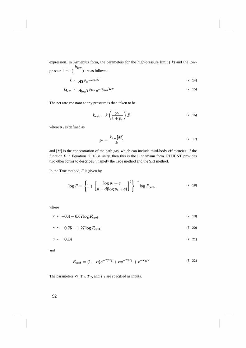
expression. In Arrhenius form, the parameters for the high-pressure limit ( k) and the low-
pressure limit ( ) are as follows:
k =
(7. 14)
=
(7. 15)
The net rate constant at any pressure is then taken to be
(7. 16)
where p r is defined as
(7. 17)
and [M] is the concentration of the bath gas, which can include third-body efficiencies. If the function F in Equation 7. 16 is unity, then this is the Lindemann form. FLUENT provides two other forms to describe F, namely the Troe method and the SRI method.
In the Troe method, F is given by
(7. 18)
where
c =
(7. 19)
n =
(7. 20)
d =
(7. 21)
and
(7. 22)
The parameters , T 3, T 2, and T 1 are specified as inputs.
92

In the SRI method, the blending function F is approximated as
(7. 23)
where
(7. 24)
In addition to the three Arrhenius parameters for the low-pressure limit ( ) expression, you must also supply the parameters a, b, c, d, and e in the F expression.
The Eddy-Dissipation Model
Most fuels are fast burning, and the overall rate of reaction is controlled by turbulent mixing. In non-premixed flames, turbulence slowly convects/mixes fuel and oxidizer into the reaction zones where they burn quickly. In premixed flames, the turbulence slowly convects/mixes cold reactants and hot products into the reaction zones, where reaction occurs rapidly. In such cases, the combustion is said to be mixing-limited, and the complex, and often unknown, chemical kinetic rates can be safely neglected.
FLUENT provides a turbulence-chemistry interaction model, based on the work of Magnussen and Hjertager [23], called the eddy-dissipation model. The net rate of production of species i due to reaction r, R i, r, is given by the smaller (i.e., limiting value) of the two expressions below:
(7. 25)
(7. 26)
where Y is the mass fraction of any product species, P P
is the mass fraction of a particular reactant,
A is an empirical constant equal to 4.0
93
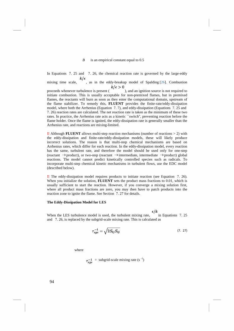
B is an empirical constant equal to 0.5
In Equations 7. 25 and 7. 26, the chemical reaction rate is governed by the large-eddy
mixing time scale, , as in the eddy-breakup model of Spalding [26]. Combustion
proceeds whenever turbulence is present ( ), and an ignition source is not required to initiate combustion. This is usually acceptable for non-premixed flames, but in premixed flames, the reactants will burn as soon as they enter the computational domain, upstream of the flame stabilizer. To remedy this, FLUENT provides the finite-rate/eddy-dissipation model, where both the Arrhenius (Equation 7. 7), and eddy-dissipation (Equations 7. 25 and 7. 26) reaction rates are calculated. The net reaction rate is taken as the minimum of these two rates. In practice, the Arrhenius rate acts as a kinetic ``switch'', preventing reaction before the flame holder. Once the flame is ignited, the eddy-dissipation rate is generally smaller than the Arrhenius rate, and reactions are mixing-limited.
!! Although FLUENT allows multi-step reaction mechanisms (number of reactions > 2) with the eddy-dissipation and finite-rate/eddy-dissipation models, these will likely produce incorrect solutions. The reason is that multi-step chemical mechanisms are based on Arrhenius rates, which differ for each reaction. In the eddy-dissipation model, every reaction has the same, turbulent rate, and therefore the model should be used only for one-step (reactant product), or two-step (reactant intermediate, intermediate product) global reactions. The model cannot predict kinetically controlled species such as radicals. To incorporate multi-step chemical kinetic mechanisms in turbulent flows, use the EDC model (described below).
!! The eddy-dissipation model requires products to initiate reaction (see Equation 7. 26). When you initialize the solution, FLUENT sets the product mass fractions to 0.01, which is usually sufficient to start the reaction. However, if you converge a mixing solution first, where all product mass fractions are zero, you may then have to patch products into the reaction zone to ignite the flame. See Section 7. 27 for details.
The Eddy-Dissipation Model for LES
When the LES turbulence model is used, the turbulent mixing rate, in Equations 7. 25 and 7. 26, is replaced by the subgrid-scale mixing rate. This is calculated as
(7. 27)
where
= subgrid-scale mixing rate (s -1)
94

S = ij
= strain rate tensor (s -1
The Eddy-Dissipation-Concept (EDC) Model
)
The eddy-dissipation-concept (EDC) model is an extension of the eddy-dissipation model to include detailed chemical mechanisms in turbulent flows [22]. It assumes that reaction occurs in small turbulent structures, called the fine scales. The volume fraction of the fine scales is modeled as [9]
(7. 28)
where *
denotes fine-scale quantities and
= volume fraction constant = 2.1377
= kinematic viscosity
Species are assumed to react in the fine structures over a time scale
(7. 29)
where is a time scale constant equal to 0.4082.
In FLUENT, combustion at the fine scales is assumed to occur as a constant pressure reactor, with initial conditions taken as the current species and temperature in the cell. Reactions proceed over the time scale , governed by the Arrhenius rates of Equation 7. 7, and are integrated numerically with the stiff ordinary differential equation solver CVODE [8]. The species state after reacting for a time is denoted by Y * i
The source term in the conservation equation for the mean species i, Equation 7. 1, is modeled as
.
(7. 30)
95

The EDC model can incorporate detailed chemical mechanisms into turbulent reacting flows. However, typical mechanisms are invariably stiff and their numerical integration is computationally costly. Hence, the model should be used only when the assumption of fast chemistry is invalid, such as modeling the slow CO burnout in rapidly quenched flames, or the NO conversion in selective non-catalytic reduction (SNCR).
The double-precision solver is recommended to avoid round-off errors that may occur as a consequence of the large pre-exponential factors and activation energies inherent in stiff mechanisms.
7.2. Overview of User Inputs for Modeling Species Transport
and Reactions
The basic steps for setting up a problem involving species transport and reactions are listed below.
1. Enable species transport and volumetric reactions, and specify the mixture material.
2. If you are also modeling wall or particle surface reactions, turn on wall surface and/or particle surface reactions as well.
3. Check and/or define the properties of the mixture. Mixture properties include the following:
• species in the mixture • reactions • other physical properties (e.g., viscosity, specific heat)
4. Check and/or set the properties of the individual species in the mixture.
5. Set species boundary conditions.
In many cases, you will not need to modify any physical properties because the solver gets species properties, reactions, etc. from the materials database when you choose the mixture material. Some properties, however, may not be defined in the database. You will be warned when you choose your material if any required properties need to be set, and you can then assign appropriate values for these properties. You may also want to check the database values of other properties to be sure that they are correct for your particular application. For details about modifying an existing mixture material or creating a new one from scratch. Modifications to the mixture material can include the following:
• Addition or removal of species • Changing the chemical reactions • Modifying other material properties for the mixture
96

• Modifying material properties for the mixture's constituent species
If you are solving a reacting flow, you will usually want to define the mixture's specific heat as a function of composition, and the specific heat of each species as a function of temperature. You may want to do the same for other properties as well. By default, constant properties are used, but for the properties of some species, there is a piecewise-polynomial function of temperature that exists in the database and is available for your use. You may also choose to specify a different temperature-dependent function if you know of one that is more suitable for your problem.
Mixture Materials
The concept of mixture materials has been implemented in FLUENT to facilitate the setup of species transport and reacting flow. A mixture material may be thought of as a set of species and a list of rules governing their interaction. The mixture material carries with it the following information:
• A list of the constituent species, referred to as ``fluid'' materials • A list of mixing laws dictating how mixture properties (density, viscosity, specific
heat, etc.) are to be derived from the properties of individual species if composition-dependent properties are desired
• A direct specification of mixture properties if composition-independent properties are desired
• Diffusion coefficients for individual species in the mixture • Other material properties (e.g., absorption and scattering coefficients) that are not
associated with individual species • A set of reactions, including a reaction type (finite-rate, eddy-dissipation, etc.) and
stoichiometry and rate constants
Both mixture materials and fluid materials are stored in the FLUENT materials database. Many common mixture materials are included (e.g., methane-air, propane-air). Generally, one/two-step reaction mechanisms and many physical properties of the mixture and its constituent species are defined in the database. When you indicate which mixture material you want to use, the appropriate mixture material, fluid materials, and properties are loaded into the solver. If any necessary information about the selected material (or the constituent fluid materials) is missing, the solver will inform you that you need to specify it. In addition, you may choose to modify any of the predefined properties. See Section 7.1.2 for information about the sources of FLUENT's database property data.
For example, if you plan to model combustion of a methane-air mixture, you do not need to explicitly specify the species involved in the reaction or the reaction itself. You will simply select methane-air as the mixture material to be used, and the relevant species (CH 4, O 2, CO 2, H 2O, and N 2) and reaction data will be loaded into the solver from the database. You can then check the species, reactions, and other properties and define any properties that are missing and/or modify any properties for which you wish to use different values or functions. You will generally want to define a composition- and temperature-dependent specific heat, and you may want to define additional properties as functions of temperature and/or composition.
97
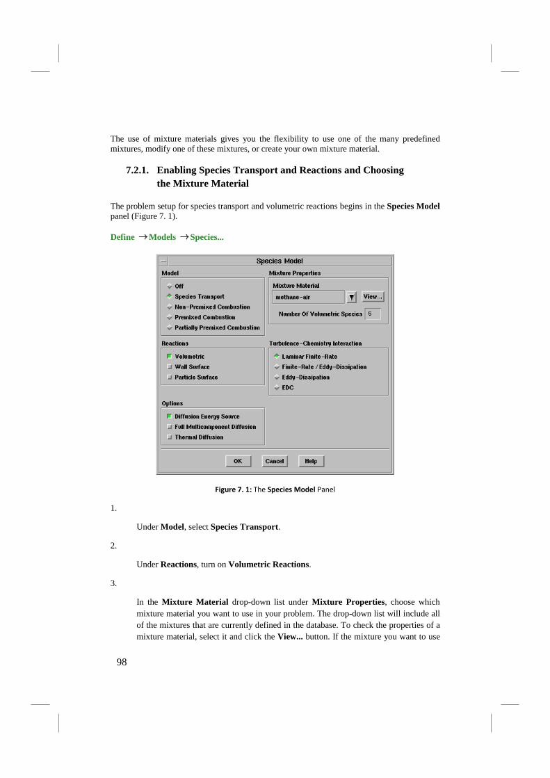
The use of mixture materials gives you the flexibility to use one of the many predefined mixtures, modify one of these mixtures, or create your own mixture material.
7.2.1. Enabling Species Transport and Reactions and Choosing the Mixture Material
The problem setup for species transport and volumetric reactions begins in the Species Model panel (Figure 7. 1).
Define Models Species...
Figure 7. 1:
1.
The Species Model Panel
Under Model, select Species Transport.
2.
Under Reactions, turn on Volumetric Reactions.
3.
In the Mixture Material drop-down list under Mixture Properties, choose which mixture material you want to use in your problem. The drop-down list will include all of the mixtures that are currently defined in the database. To check the properties of a mixture material, select it and click the View... button. If the mixture you want to use
98

is not in the list, choose the mixture-template material,. If there is a mixture material listed that is similar to your desired mixture, you may choose that material on modifying properties of an existing material.
When you choose the Mixture Material, the Number of Volumetric Species in the mixture will be displayed in the panel for your information.
4.
Choose the Turbulence-Chemistry Interaction model. Four models are available:
Laminar Finite-Rate
computes only the Arrhenius rate (see Equation 7. 7) and neglects turbulence-chemistry interaction.
Eddy-Dissipation
(for turbulent flows) computes only the mixing rate (see Equations 7. 25 and 7. 26).
Finite-Rate/Eddy-Dissipation
(for turbulent flows) computes both the Arrhenius rate and the mixing rate and uses the smaller of the two.
EDC
(for turbulent flows) models turbulence-chemistry interaction with detailed chemical mechanisms (see Equations 7. 25 and 7. 26).
5.
If you selected EDC, you have the option to modify the Volume Fraction Constant
and the Time Scale Constant ( in Equation 7. 28 and in Equation 7. 29), although the default values are recommended. Further, to reduce the computational expense of the chemistry calculations, you can increase the number of Flow Iterations Per Chemistry Update. By default, FLUENT will update the chemistry one per 10 flow iterations.
6.
(optional) If you want to model full multicomponent diffusion or thermal diffusion, turn on the Full Multicomponent Diffusion or Thermal Diffusion option.
99

7.2.2. Defining Properties for the Mixture and Its Constituent Species
Remember that you will need to define properties for the mixture material and also for its constituent species. It is important that you define the mixture properties before setting any properties for the constituent species, since the species property inputs may depend on the methods you use to define the properties of the mixture. The recommended sequence for property inputs is as follows:
1.
Define the mixture species, and reaction(s), and define physical properties for the mixture. Remember to click on the Change/Create button when you are done setting properties for the mixture material.
2.
Define physical properties for the species in the mixture. Remember to click on the Change/Create button after defining the properties for each species.
Define Materials...
Defining the Species in the Mixture
If you are using a mixture material from the database, the species in the mixture will already be defined for you. If you are creating your own material or modifying the species in an existing material, you will need to define them yourself.
In the Materials panel (Figure 7.2), check that the Material Type is set to mixture and your mixture is selected in the Mixture Materials list. Click on the Edit... button to the right of Mixture Species to open the Species panel (Figure 7.3).
100

Figure 7.2: The Materials Panel (showing a mixture material)
Figure 7.3: The Species Panel
101
Overview of the Species Panel
In the Species panel, the Selected Species list shows all of the fluid-phase species in the mixture. If you are modeling wall or particle surface reactions, the Selected Surface Species list will show all of the surface species in the mixture. Surface species are species that are created or evolved from wall boundaries or discrete-phase particles (e.g., Si(s)) and do not exist as fluid-phase species.
!! The order of the species in the Selected Species list is very important. FLUENT considers the last species in the list to be the bulk species. You should therefore be careful to retain the most abundant species (by mass) as the last species when you add species to or delete species from a mixture material.
The Available Materials list shows materials that are available but not in the mixture. Generally you will see air in this list, since air is always available by default.
Adding Species to the Mixture
If you are creating a mixture from scratch or starting from an existing mixture and adding some missing species, you will first need to load the desired species from the database (or create them, if they are not present in the database) so that they will be available to the solver. The procedure for adding species is listed below. (You will need to close the Species panel before you begin, since it is a ``modal'' panel that will not allow you to do anything else when it is open.)
1.
In the Materials panel, click on the Database... button to open the Database Materials panel and copy the desired species. Remember that the constituent species of the mixture are fluid materials, so you should select fluid as the Material Type in the Database Materials panel to see the correct list of choices. Note that available solid species (for surface reactions) are also contained in the fluid list.
!! If you do not see the species you are looking for in the database, you can create a new fluid material for that species, and then continue with step 2, below.
2.
Re-open the Species panel, as described above. You will see that the fluid materials you copied from the database (or created) are listed in the Available Materials list.
3.
To add a species to the mixture, select it in the Available Materials list and click on the Add button below the Selected Species list (or below the Selected Surface Species list, to define a surface species). The species will be added to the end of the Selected Species (or Selected Surface Species) list and removed from the Available Materials list.
102

4.
Repeat the previous step for all the desired species. When you are finished, click on the OK button.
!! Adding a species to the list will alter the order of the species. You should be sure that the last species in the list is the bulk species, and you should check any boundary conditions, under-relaxation factors, or other solution parameters that you have set, as described in detail below.
Removing Species from the Mixture
To remove a species from the mixture, simply select it in the Selected Species list (or the Selected Surface Species list) and click on the Remove button below the list. The species will be removed from the list and added to the Available Materials list.
!! Removing a species from the list will alter the order of the species. You should be sure that the last species in the list is the bulk species, and you should check any boundary conditions, under-relaxation factors, or other solution parameters that you have set, as described in detail below.
Reordering Species
If you find that the last species in the Selected Species list is not the most abundant species (as it must be), you will need to rearrange the species to obtain the proper order.
1.
Remove the bulk species from the Selected Species list. It will now appear in the Available Species list.
2.
Add the species back in again. It will automatically be placed at the end of the list.
The Naming and Ordering of Species
As discussed above, you must retain the most abundant species as the last one in the Selected Species list when you add or remove species. Additional considerations you should be aware of when adding and deleting species are presented here.
There are three characteristics of a species that identify it to the solver: name, chemical formula, and position in the list of species in the Species panel. Changing these characteristics will have the following effects:
• You can change the Name of a species without any consequences. • You should never• You will change the order of the species list if you add or remove any species. When this
occurs, all boundary conditions, solver parameters, and solution data for species will be reset to the default values. (Solution data, boundary conditions, and solver parameters for other flow variables will not be affected.) Thus, if you add or remove species you should take care
change the given Chemical Formula of a species.
103
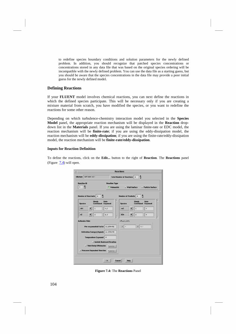
to redefine species boundary conditions and solution parameters for the newly defined problem. In addition, you should recognize that patched species concentrations or concentrations stored in any data file that was based on the original species ordering will be incompatible with the newly defined problem. You can use the data file as a starting guess, but you should be aware that the species concentrations in the data file may provide a poor initial guess for the newly defined model.
Defining Reactions
If your FLUENT model involves chemical reactions, you can next define the reactions in which the defined species participate. This will be necessary only if you are creating a mixture material from scratch, you have modified the species, or you want to redefine the reactions for some other reason.
Depending on which turbulence-chemistry interaction model you selected in the Species Model panel, the appropriate reaction mechanism will be displayed in the Reaction drop-down list in the Materials panel. If you are using the laminar finite-rate or EDC model, the reaction mechanism will be finite-rate; if you are using the eddy-dissipation model, the reaction mechanism will be eddy-dissipation; if you are using the finite-rate/eddy-dissipation model, the reaction mechanism will be finite-rate/eddy-dissipation.
Inputs for Reaction Definition
To define the reactions, click on the Edit... button to the right of Reaction. The Reactions panel (Figure 7.4) will open.
Figure 7.4: The Reactions Panel
104
The steps for defining reactions are as follows:
1.
Set the total number of reactions (volumetric reactions, wall surface reactions, and particle surface reactions) in the Total Number of Reactions field. (Use the arrows to change the value, or type in the value and press RETURN
Note that if your model includes discrete-phase combusting particles, you should include the particulate surface reaction(s) (e.g., char burnout, multiple char oxidation) in the number of reactions
.)
only
2.
if you plan to use the multiple surface reactions model for surface combustion.
Set the Reaction ID of the reaction you want to define. (Again, if you type in the value be sure to press RETURN
3.
.)
If this is a fluid-phase reaction, keep the default selection of Volumetric as the Reaction Type. If this is a wall surface reaction or a particle surface reaction, select Wall Surface or Particle Surface as the Reaction Type
4.
Specify how many reactants and products are involved in the reaction by increasing the value of the Number of Reactants and the Number of Products. Select each reactant or product in the Species drop-down list and then set its stoichiometric coefficient and rate exponent in the appropriate Stoich. Coefficient and Rate Exponent fields. (The stoichiometric coefficient is
the constant or in Equation 7. 6 and the rate exponent is the exponent on the
reactant or product concentration, or in Equation 7. 7.)
There are two general classes of reactions that can be handled by the Reactions panel, so it is important that the parameters for each reaction are entered correctly. The classes of reactions are as follows:
• Global forward reaction (no reverse reaction): Product species generally do not affect
the forward rate, so the rate exponent for all products ( ) should be 0. For reactant
species, set the rate exponent ( ) to the desired value. If such a reaction is not an elementary reaction, the rate exponent will generally not be equal to the stoichiometric
coefficient ( ) for that species. An example of a global forward reaction is the combustion of methane:
105

(7. 31)
where , , , , ,
, , and .
Note that, in certain cases, you may wish to model a reaction where product species affect the forward rate. For such cases, set the product rate exponent (
) to the desired value. An example of such a reaction is the gas-shift reaction (see the carbon-monoxide-air mixture material in the Database Materials panel), in which the presence of water has an effect on the reaction rate:
(7. 32)
In the gas-shift reaction, the rate expression may be defined as:
(7. 33)
where , , , , ,
, , and .
• Reversible reaction: An elementary chemical reaction that assumes the rate exponent for each species is equivalent to the stoichiometric coefficient for that species. An example of an elementary reaction is the oxidation of SO 2 to SO 3:
(7. 34)
where , , , , , and
.
See step 6 below for information about how to enable reversible reactions.
106
5.
If you are using the laminar finite-rate, finite-rate/eddy-dissipation, or EDC model for the turbulence-chemistry interaction, enter the following parameters for the Arrhenius rate under the Arrhenius Rate heading:
Pre-exponential Factor
(the constant A r in Equation 7. 9). The units of A r must be specified such that the units of the
molar reaction rate, in Equation 7. 5, are moles/volume-time (e.g., kgmol/m 3-s) and the units of the volumetric reaction rate, R i in Equation 7. 6, are mass/volume-time (e.g., kg/m 3
!! It is important to note that if you have selected the British units system, the Arrhenius factor should still be input in SI units. This is because FLUENT applies no conversion factor to your input of A
-s).
r (the conversion factor is 1.0) when you work in
British units, as the correct conversion factor depends on your inputs for , , etc.
Activation Energy
(the constant E r
Temperature Exponent
in the forward rate constant expression, Equation 7. 9).
(the value for the constant in Equation 7. 9).
Third Body Efficiencies
(the values for in Equation 7. 8). If you have accurate data for the efficiencies and want to include this effect on the reaction rate (i.e., include in Equation 7. 7), turn on the Third Body Efficiencies option and click on the Specify... button to open the Reaction Parameters panel (Figure 7.5). For each Species in the panel, specify the Third-body Efficiency.
107

Figure 7.5:
!! It is not necessary to include the third-body efficiencies. You should not enable the Third Body Efficiencies option unless you have accurate data for these parameters.
The Reaction Parameters Panel
Pressure Dependent Reaction
(if relevant) If you are using the laminar finite-rate or EDC model for turbulence-chemistry interaction, and the reaction is a pressure fall-off reaction, turn on the Pressure Dependent Reaction option for the Arrhenius Rate and click on the Specify... button to open the Pressure-Dependent Reaction panel (Figure 7.6).
108
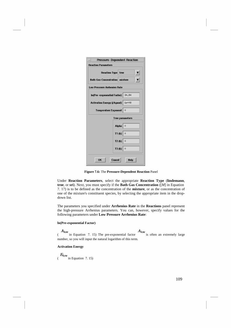
Figure 7.6:
Under Reaction Parameters, select the appropriate Reaction Type (lindemann, troe, or sri). Next, you must specify if the Bath Gas Concentration ([M] in Equation 7. 17) is to be defined as the concentration of the mixture, or as the concentration of one of the mixture's constituent species, by selecting the appropriate item in the drop-down list.
The Pressure-Dependent Reaction Panel
The parameters you specified under Arrhenius Rate in the Reactions panel represent the high-pressure Arrhenius parameters. You can, however, specify values for the following parameters under Low Pressure Arrhenius Rate:
ln(Pre-exponential Factor)
( in Equation 7. 15) The pre-exponential factor is often an extremely large number, so you will input the natural logarithm of this term.
Activation Energy
( in Equation 7. 15)
109
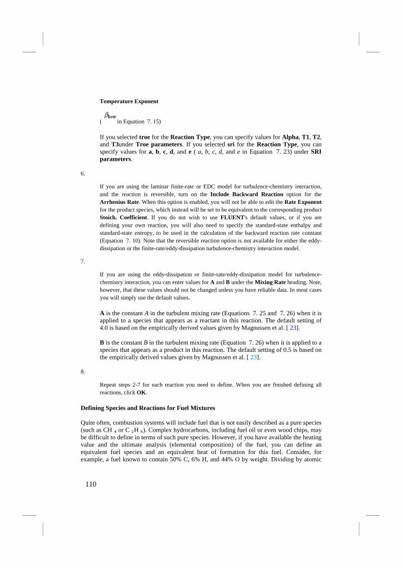
Temperature Exponent
( in Equation 7. 15)
If you selected troe for the Reaction Type, you can specify values for Alpha, T1, T2, and T3under Troe parameters. If you selected sri for the Reaction Type, you can specify values for a, b, c, d, and e ( a, b, c, d, and e in Equation 7. 23) under SRI parameters.
6.
If you are using the laminar finite-rate or EDC model for turbulence-chemistry interaction, and the reaction is reversible, turn on the Include Backward Reaction option for the Arrhenius Rate. When this option is enabled, you will not be able to edit the Rate Exponent for the product species, which instead will be set to be equivalent to the corresponding product Stoich. Coefficient. If you do not wish to use FLUENT's default values, or if you are defining your own reaction, you will also need to specify the standard-state enthalpy and standard-state entropy, to be used in the calculation of the backward reaction rate constant (Equation 7. 10). Note that the reversible reaction option is not available for either the eddy-dissipation or the finite-rate/eddy-dissipation turbulence-chemistry interaction model.
7.
If you are using the eddy-dissipation or finite-rate/eddy-dissipation model for turbulence-chemistry interaction, you can enter values for A and B under the Mixing Rate heading. Note, however, that these values should not be changed unless you have reliable data. In most cases you will simply use the default values.
A is the constant A in the turbulent mixing rate (Equations 7. 25 and 7. 26) when it is applied to a species that appears as a reactant in this reaction. The default setting of 4.0 is based on the empirically derived values given by Magnussen et al. [ 23].
B is the constant B in the turbulent mixing rate (Equation 7. 26) when it is applied to a species that appears as a product in this reaction. The default setting of 0.5 is based on the empirically derived values given by Magnussen et al. [ 23].
8.
Repeat steps 2-7 for each reaction you need to define. When you are finished defining all reactions, click OK.
Defining Species and Reactions for Fuel Mixtures
Quite often, combustion systems will include fuel that is not easily described as a pure species (such as CH 4 or C 2H 6). Complex hydrocarbons, including fuel oil or even wood chips, may be difficult to define in terms of such pure species. However, if you have available the heating value and the ultimate analysis (elemental composition) of the fuel, you can define an equivalent fuel species and an equivalent heat of formation for this fuel. Consider, for example, a fuel known to contain 50% C, 6% H, and 44% O by weight. Dividing by atomic
110
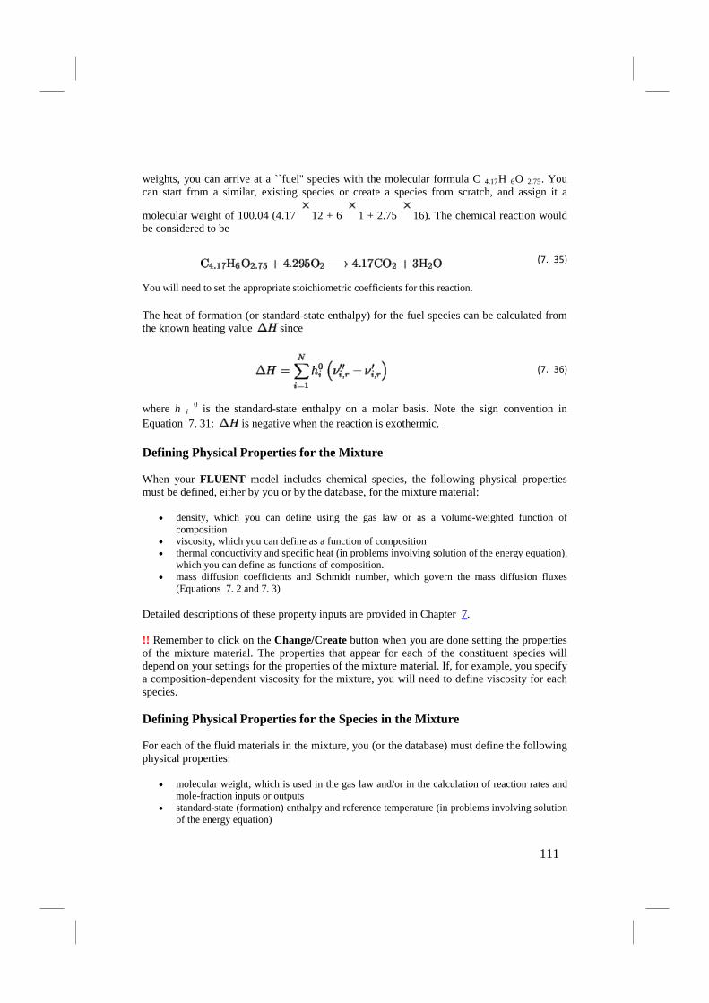
weights, you can arrive at a ``fuel'' species with the molecular formula C 4.17H 6O 2.75. You can start from a similar, existing species or create a species from scratch, and assign it a
molecular weight of 100.04 (4.17 12 + 6 1 + 2.75 16). The chemical reaction would be considered to be
(7. 35)
You will need to set the appropriate stoichiometric coefficients for this reaction.
The heat of formation (or standard-state enthalpy) for the fuel species can be calculated from the known heating value since
(7. 36)
where h i 0 is the standard-state enthalpy on a molar basis. Note the sign convention in Equation 7. 31: is negative when the reaction is exothermic.
Defining Physical Properties for the Mixture
When your FLUENT model includes chemical species, the following physical properties must be defined, either by you or by the database, for the mixture material:
• density, which you can define using the gas law or as a volume-weighted function of composition
• viscosity, which you can define as a function of composition • thermal conductivity and specific heat (in problems involving solution of the energy equation),
which you can define as functions of composition. • mass diffusion coefficients and Schmidt number, which govern the mass diffusion fluxes
(Equations 7. 2 and 7. 3)
Detailed descriptions of these property inputs are provided in Chapter 7.
!! Remember to click on the Change/Create button when you are done setting the properties of the mixture material. The properties that appear for each of the constituent species will depend on your settings for the properties of the mixture material. If, for example, you specify a composition-dependent viscosity for the mixture, you will need to define viscosity for each species.
Defining Physical Properties for the Species in the Mixture
For each of the fluid materials in the mixture, you (or the database) must define the following physical properties:
• molecular weight, which is used in the gas law and/or in the calculation of reaction rates and mole-fraction inputs or outputs
• standard-state (formation) enthalpy and reference temperature (in problems involving solution of the energy equation)
111

• viscosity, if you defined the viscosity of the mixture material as a function of composition • thermal conductivity and specific heat (in problems involving solution of the energy equation),
if you defined these properties of the mixture material as functions of composition • standard-state entropy, if you are modeling reversible reactions
Detailed descriptions of these property inputs are provided in Chapter 7.
!! Global reaction mechanisms with one or two steps inevitably neglect the intermediate species. In high-temperature flames, neglecting these dissociated species may cause the temperature to be overpredicted. A more realistic temperature field can be obtained by increasing the specific heat capacity for each species. Rose and Cooper [28] have created a set of specific heat polynomials as a function of temperature. The specific heat capacity for each species is calculated as
(7. 37)
The modified c p polynomial coefficients from [28] are provided in Table 7.1.
Table 7.1: Modified c p Polynomial Coefficients [28]
N CH 2 CO 4 H 2
a 0 1.02705e+03 2.00500e+03 1.04669e+03
1.4147e+04
a 1 2.16182e-02
-6.81428e-01 -1.56841e-01 1.7372e-01
a 2 1.48638e-04 7.08589e-03 5.39904e-04
6.9e-04
a -4.48421e-08 3 -4.71368e-06 -3.01061e-07 ---
a --- 4 8.51317e-10 5.05048e-11
---
CO H 2 2 O O 2
a 0 5.35446e+02 1.93780e+03 8.76317e+02
112
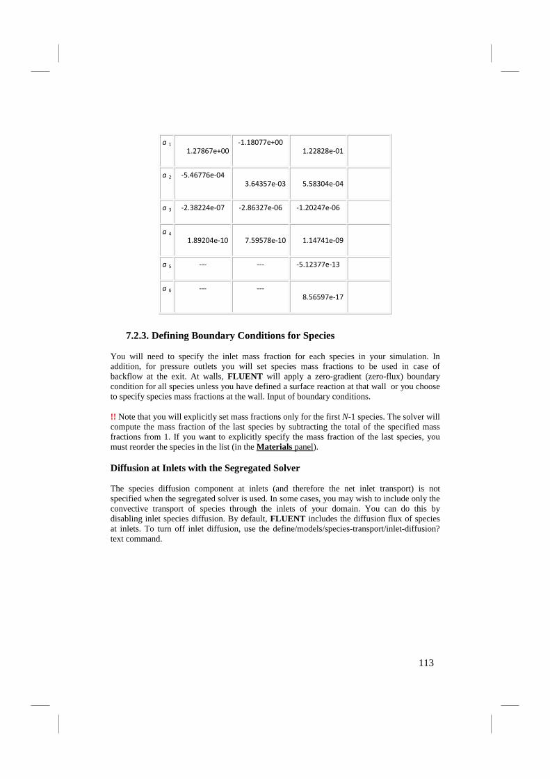
a 1 1.27867e+00
-1.18077e+00 1.22828e-01
a -5.46776e-04 2 3.64357e-03 5.58304e-04
a -2.38224e-07 3 -2.86327e-06 -1.20247e-06
a 4 1.89204e-10 7.59578e-10 1.14741e-09
a --- 5 --- -5.12377e-13
a --- 6 --- 8.56597e-17
7.2.3. Defining Boundary Conditions for Species
You will need to specify the inlet mass fraction for each species in your simulation. In addition, for pressure outlets you will set species mass fractions to be used in case of backflow at the exit. At walls, FLUENT will apply a zero-gradient (zero-flux) boundary condition for all species unless you have defined a surface reaction at that wall or you choose to specify species mass fractions at the wall. Input of boundary conditions.
!! Note that you will explicitly set mass fractions only for the first N-1 species. The solver will compute the mass fraction of the last species by subtracting the total of the specified mass fractions from 1. If you want to explicitly specify the mass fraction of the last species, you must reorder the species in the list (in the Materials panel).
Diffusion at Inlets with the Segregated Solver
The species diffusion component at inlets (and therefore the net inlet transport) is not specified when the segregated solver is used. In some cases, you may wish to include only the convective transport of species through the inlets of your domain. You can do this by disabling inlet species diffusion. By default, FLUENT includes the diffusion flux of species at inlets. To turn off inlet diffusion, use the define/models/species-transport/inlet-diffusion? text command.
113

7.3. Theory
The Arrhenius Rate for Wall Surface Reactions
Consider the rth wall surface reaction written in general form as follows:
(7. 37)
where N = total number of chemical species in the system
= stoichiometric coefficient for reactant i in
reaction r
= stoichiometric coefficient for product i in
reaction r
= symbol denoting species i
k = f, r forward rate constant for reaction r
The summations in Equation 7. 1 are for all chemical species in the system, but only species involved as reactants or products will have non-zero stoichiometric coefficients. Hence, species that are not involved will drop out of the equation.
The molar rate of creation/destruction of species i in reaction r ( in Equation 7. 5) is given by
114

(7. 38)
where N = r number of chemical species in reaction r
C = j, r molar concentration of each reactant and product
species j in reaction r (kgmol/m 3
)
= forward rate exponent for each reactant and product
species j in reaction r
The forward rate constant for reaction r, k f, r
, is computed using the Arrhenius expression
(7. 39)
where A = r pre-exponential factor (consistent units)
= temperature exponent (dimensionless)
E = r activation energy for the reaction (J/kgmol)
R = universal gas constant (J/kgmol-K)
You (or the database) will provide values for , , , , A r, and E r.
Wall Surface Reaction Boundary Conditions
For wall surface reactions, the calculation of the species concentration at reacting surfaces is based on a balance of the convection and diffusion of each species to (or from) the surface
115
and the rate at which it is consumed (or produced) at the surface. This flux balance for species i can be written as
(7. 40)
where is a unit vector normal to the surface
is the diffusion flux of species i
R'' i
is the rate of production of species i due to surface reaction
is the total mass deposition rate
is the mass fraction of species i at the wall
Using Equation 7. 4, expressions can be derived for the mass fraction of species i at the wall and for the net rate of creation of species i per unit area. These expressions are used in FLUENT to compute gas-phase species concentrations at reacting surfaces using a point-by-point coupled stiff solver.
Including Mass Transfer To Surfaces in Continuity
In the surface reaction boundary condition described above, the effects of the wall normal velocity or bulk mass transfer to the wall are not included in the computation of species transport. The momentum of the net surface mass flux from the surface is also ignored because the momentum flux through the surface is usually small in comparison with the momentum of the flow in the cells adjacent to the surface. However, you can include the effect of surface mass transfer in the continuity equation by activating the Mass Deposition Source option in the
Species Model panel.
Wall Surface Mass Transfer Effects in the Energy Equation
Species diffusion effects in the energy equation due to wall surface reactions are included in the normal species diffusion term.
If you are using the segregated solver, you can neglect this term by turning off the Diffusion Energy Source option in the Species Model panel. (For the coupled solvers, this term is always included; you cannot turn it off.) Neglecting the species diffusion term implies that
116
errors may be introduced to the prediction of temperature in problems involving mixing of species with significantly different heat capacities, especially for components with a Lewis number far from unity. While the effect of species diffusion should go to zero at Le = 1, you may see subtle effects due to differences in the numerical integration in the species and energy equations.
Modeling the Heat Release Due to Wall Surface Reactions
The heat release due to a wall surface reaction is, by default, ignored by FLUENT. You can, however, choose to include the heat of surface reaction by activating the Heat of Surface Reactions option in the
Species Model panel and setting appropriate formation enthalpies in the Materials panel.
7.4. Species Transport Without Reactions
In addition to the volumetric and surface reactions described in the previous sections, you can also use FLUENT to solve a species mixing problem without reactions. The species transport equations that FLUENT will solve are described in Section 7, and the procedure you will follow to set up the non-reacting species transport problem is the same as that described in Sections 7. 1. 2, with some simplifications.
The basic steps are listed below:
1. Enable Species Transport in the Species Model panel and select the appropriate Mixture Material.
Define Models Species...
2. (optional) If you want to model full multicomponent diffusion or thermal diffusion, turn on the Full Multicomponent Diffusion or Thermal Diffusion option
3. Check and/or define the properties of the mixture and its constituent species.
Define Materials...
Mixture properties include the following:
• species in the mixture • other physical properties (e.g., viscosity, specific heat)
4. Set species boundary conditions.
No special solution procedures are usually required for a non-reacting species transport calculation. Upon completion of the calculation, you can display or report the following quantities:
117

• Mass fraction of species-n • Mole fraction of species-n • Concentration of species-n • Lam Diff Coef of species-n • Eff Diff Coef of species-n • Enthalpy of species-n (segregated solver calculations only) • Relative Humidity
These variables are contained in the Species... category of the variable selection drop-down list that appears in postprocessing panels.
7.5. Modeling Non-Premixed Combustion
In non-premixed combustion, fuel and oxidizer enter the reaction zone in distinct streams. This is in contrast to premixed systems, in which reactants are mixed at the molecular level before burning. Examples of non-premixed combustion include methane combustion, pulverized coal furnaces, and diesel (compression) internal-combustion engines.
Under certain assumptions, the thermochemistry can be reduced to a single parameter: the mixture fraction. The mixture fraction, denoted by f, is the mass fraction that originated from the fuel stream. In other words, it is the local mass fraction of burnt and unburnt fuel stream elements (C, H, etc.) in all the species (CO 2, H 2O, O 2
, etc.). The approach is elegant because atomic elements are conserved in chemical reactions. In turn, the mixture fraction is a conserved scalar quantity, and therefore its governing transport equation does not have a source term. Combustion is simplified to a mixing problem, and the difficulties associated with closing non-linear mean reaction rates are avoided. Once mixed, the chemistry can be modeled as in chemical equilibrium, or near chemical equilibrium with the laminar flamelet model.
7.5.1. Description of the Equilibrium Mixture Fraction/ PDF Model
The non-premixed modeling approach involves the solution of transport equations for one or two conserved scalars (the mixture fractions). Equations for individual species are not solved. Instead, species concentrations are derived from the predicted mixture fraction fields. The thermochemistry calculations are preprocessed in prePDF and tabulated for look-up in FLUENT. Interaction of turbulence and chemistry is accounted for with a probability density function (PDF).
7.5.2. Benefits and Limitations of the Non-Premixed Approach
Advantages of the Non-Premixed Approach
The non-premixed modeling approach has been specifically developed for the simulation of turbulent diffusion flames with fast chemistry. The non-premixed model allows intermediate (radical) species prediction, dissociation effects, and rigorous turbulence-chemistry coupling. The method is computationally efficient in that it does not require the solution of a large number of species transport equations. When the underlying assumptions are valid, the non-premixed approach is preferred over the finite rate formulation.
118

Limitations of the Non-Premixed Approach
The non-premixed approach can be used only when your reacting flow system meets several requirements. First, the FLUENT implementation requires that the flow be turbulent. Second, the reacting system includes a fuel stream, an oxidant stream, and, optionally, a secondary stream (another fuel or oxidant, or a non-reacting stream). Finally, the chemical kinetics must be rapid so that the flow is near chemical equilibrium.
!! Note that the non-premixed model can be used only with the segregated solver; it is not available with the coupled solvers.
7.5.3. Details of the Non-Premixed Approach
Definition of the Mixture Fraction
The basis of the non-premixed modeling approach is that under a certain set of simplifying assumptions, the instantaneous thermochemical state of the fluid is related to a conserved scalar quantity known as the mixture fraction f. The mixture fraction can be written in terms of the atomic mass fraction as [
213]
(7. 41)
where Z i is the elemental mass fraction for some element, i. The subscript ox denotes the value at the oxidizer stream inlet and the subscript fuel denotes the value at the fuel stream inlet. If the diffusion coefficients for all species are equal, then Equation 7. 41 is identical for all elements, and the mixture fraction definition is unique. The mixture fraction is thus the elemental mass fraction that originated from the fuel stream. Note that this mass fraction includes all elements from the fuel stream, including inert species such as N 2, and any oxidizing species mixed with the fuel, such as O 2
If a secondary stream (another fuel or oxidant, or a non-reacting stream) is included, the fuel and secondary mixture fractions are simply the mass fractions of the fuel and secondary streams. The sum of all three mixture fractions in the system (fuel, secondary stream, and oxidizer) is always equal to 1:
.
(7. 42)
This indicates that only points on the plane ABC (shown in Figure 7. 7) in the mixture
fraction space are valid. Consequently, the two mixture fractions, and , cannot vary independently; their values are valid only if they are both within the triangle OBC shown in Figure 7. 8.
119
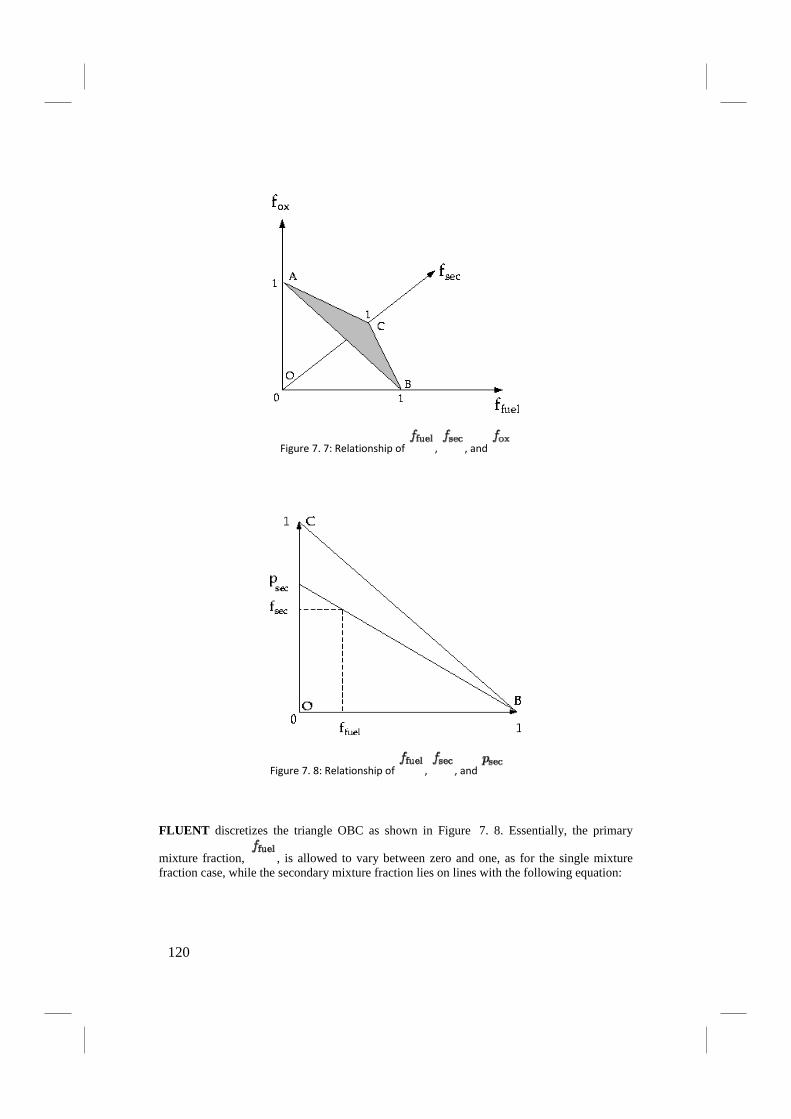
Figure 7. 7: Relationship of , , and
Figure 7. 8: Relationship of , , and
FLUENT discretizes the triangle OBC as shown in Figure 7. 8. Essentially, the primary
mixture fraction, , is allowed to vary between zero and one, as for the single mixture fraction case, while the secondary mixture fraction lies on lines with the following equation:
120

(7. 43)
where is the normalized secondary mixture fraction and is the value at the intersection of
a line with the secondary mixture fraction axis. Note that unlike , is bounded
between zero and one, regardless of the value.
An important characteristic of the normalized secondary mixture fraction, , is its assumed
statistical independence from the fuel mixture fraction, . Note that unlike , is not a conserved scalar. The normalized mixture fraction definition for the second scalar variable is used everywhere except when defining the rich limit for a secondary fuel stream,
which is defined in terms of .
Transport Equations for the Mixture Fraction
Under the assumption of equal diffusivities, the species equations can be reduced to a single equation for the mixture fraction, f. The reaction source terms in the species equations cancel, and thus f is a conserved quantity. While the assumption of equal diffusivities is problematic for laminar flows, it is generally acceptable for turbulent flows where turbulent convection overwhelms molecular diffusion. The mean (time-averaged) mixture fraction equation is
(7. 44)
The source term S m is due solely to transfer of mass into the gas phase from liquid fuel
droplets or reacting particles (e.g., coal). is any user-defined source term.
In addition to solving for the mean mixture fraction, FLUENT solves a conservation equation
for the mean mixture fraction variance, [11]:
(7. 45)
121

where . The constants , C g, and C d take the values 0.85, 2.86, and 2.0,
respectively, and is any user-defined source term.
The mixture fraction variance is used in the closure model describing turbulence-chemistry interactions.
For a two-mixture-fraction problem, and are obtained from Equations 7. 44 and 7.
45 by substituting for and for . is obtained from Equation 7. 44 by
substituting for . is then calculated using Equation 7. 43, and is obtained by
solving Equation 7. 45 with substituted for . Solution for instead of is justified by the fact that the amount of the secondary stream is relatively small compared with
the total mass flow rate. To a first-order approximation, the variances in and are
relatively insensitive to , and therefore is essentially the same as .
The Non-Premixed Model for LES
For large eddy simulations (LES), an equation for the mean mixture fraction is solved, which
is identical in form to Equation 7. 44 except that is the subgrid-scale viscosity.
A transport equation is not solved for the mixture fraction variance. Instead, it is modeled as
(7. 46)
where
= user-adjustable constant
= subgrid length scale
122

Mixture Fraction vs. Equivalence Ratio
The mixture fraction definition can be understood in relation to common measures of reacting systems. Consider a simple combustion system involving a fuel stream (F), an oxidant stream (O), and a product stream (P) symbolically represented at stoichiometric conditions as
(7. 47)
where r is the air-to-fuel ratio on a mass basis. Denoting the equivalence ratio as , where
(7. 48)
the reaction in Equation 7.47, under more general mixture conditions, can then be written as
(7. 49)
Looking at the left side of this equation, the mixture fraction for the system as a whole can then be deduced to be
(7. 50)
Equation 7. 50 is an important result, allowing the computation of the mixture fraction at
stoichiometric conditions ( = 1) or at fuel-rich conditions (e.g., > 2).
Relationship of f to Species Mass Fraction, Density, and Temperature
The power of the mixture fraction modeling approach is that the chemistry is reduced to one or two conserved mixture fractions. All thermochemical scalars (species mass fraction, density, and temperature) are uniquely related to the mixture fraction(s). Given a description of the reacting system chemistry, and certain other restrictions on the system, the instantaneous mixture fraction value at each point in the flow field can be used to compute the instantaneous values of individual species mole fractions, density, and temperature.
If, in addition, the reacting system is adiabatic, the instantaneous values of mass fractions, density, and temperature depend solely on the instantaneous mixture fraction, f:
123
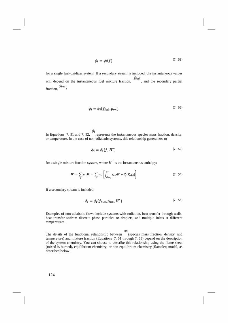
(7. 51)
for a single fuel-oxidizer system. If a secondary stream is included, the instantaneous values
will depend on the instantaneous fuel mixture fraction, , and the secondary partial
fraction, :
(7. 52)
In Equations 7. 51 and 7. 52, represents the instantaneous species mass fraction, density, or temperature. In the case of non-adiabatic systems, this relationship generalizes to
(7. 53)
for a single mixture fraction system, where H * is the instantaneous enthalpy:
(7. 54)
If a secondary stream is included,
(7. 55)
Examples of non-adiabatic flows include systems with radiation, heat transfer through walls, heat transfer to/from discrete phase particles or droplets, and multiple inlets at different temperatures.
The details of the functional relationship between (species mass fraction, density, and temperature) and mixture fraction (Equations 7. 51 through 7. 55) depend on the description of the system chemistry. You can choose to describe this relationship using the flame sheet (mixed-is-burned), equilibrium chemistry, or non-equilibrium chemistry (flamelet) model, as described below.
124
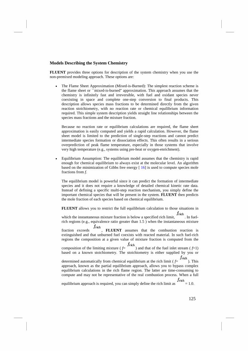
Models Describing the System Chemistry
FLUENT provides three options for description of the system chemistry when you use the non-premixed modeling approach. These options are:
• The Flame Sheet Approximation (Mixed-is-Burned): The simplest reaction scheme is the flame sheet or ``mixed-is-burned'' approximation. This approach assumes that the chemistry is infinitely fast and irreversible, with fuel and oxidant species never coexisting in space and complete one-step conversion to final products. This description allows species mass fractions to be determined directly from the given reaction stoichiometry, with no reaction rate or chemical equilibrium information required. This simple system description yields straight line relationships between the species mass fractions and the mixture fraction.
Because no reaction rate or equilibrium calculations are required, the flame sheet approximation is easily computed and yields a rapid calculation. However, the flame sheet model is limited to the prediction of single-step reactions and cannot predict intermediate species formation or dissociation effects. This often results in a serious overprediction of peak flame temperature, especially in those systems that involve very high temperature (e.g., systems using pre-heat or oxygen-enrichment).
• Equilibrium Assumption: The equilibrium model assumes that the chemistry is rapid enough for chemical equilibrium to always exist at the molecular level. An algorithm based on the minimization of Gibbs free energy [ 16] is used to compute species mole fractions from f.
The equilibrium model is powerful since it can predict the formation of intermediate species and it does not require a knowledge of detailed chemical kinetic rate data. Instead of defining a specific multi-step reaction mechanism, you simply define the important chemical species that will be present in the system. FLUENT then predicts the mole fraction of each species based on chemical equilibrium.
FLUENT allows you to restrict the full equilibrium calculation to those situations in
which the instantaneous mixture fraction is below a specified rich limit, . In fuel-rich regions (e.g., equivalence ratio greater than 1.5 ) when the instantaneous mixture
fraction exceeds , FLUENT assumes that the combustion reaction is extinguished and that unburned fuel coexists with reacted material. In such fuel-rich regions the composition at a given value of mixture fraction is computed from the
composition of the limiting mixture ( f= ) and that of the fuel inlet stream ( f=1) based on a known stoichiometry. The stoichiometry is either supplied by you or
determined automatically from chemical equilibrium at the rich limit ( f= ). This approach, known as the partial equilibrium approach, allows you to bypass complex equilibrium calculations in the rich flame region. The latter are time-consuming to compute and may not be representative of the real combustion process. When a full
equilibrium approach is required, you can simply define the rich limit as = 1.0.
125
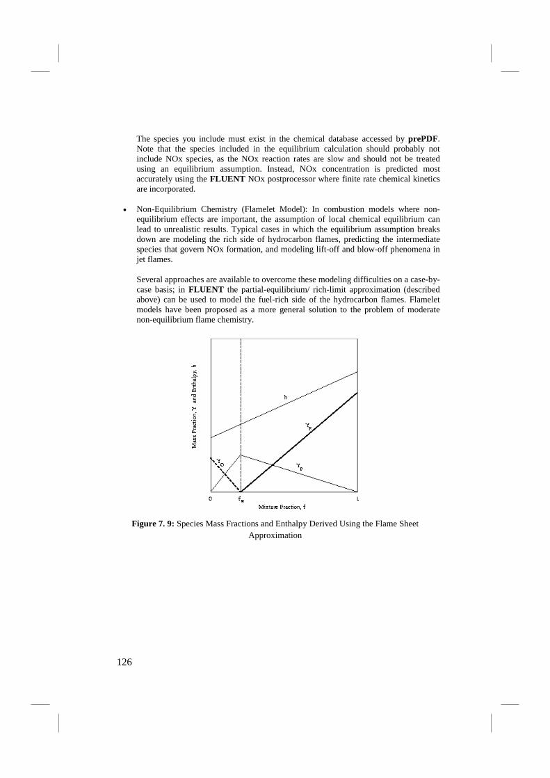
The species you include must exist in the chemical database accessed by prePDF. Note that the species included in the equilibrium calculation should probably not include NOx species, as the NOx reaction rates are slow and should not be treated using an equilibrium assumption. Instead, NOx concentration is predicted most accurately using the FLUENT NOx postprocessor where finite rate chemical kinetics are incorporated.
• Non-Equilibrium Chemistry (Flamelet Model): In combustion models where non-equilibrium effects are important, the assumption of local chemical equilibrium can lead to unrealistic results. Typical cases in which the equilibrium assumption breaks down are modeling the rich side of hydrocarbon flames, predicting the intermediate species that govern NOx formation, and modeling lift-off and blow-off phenomena in jet flames.
Several approaches are available to overcome these modeling difficulties on a case-by-case basis; in FLUENT the partial-equilibrium/ rich-limit approximation (described above) can be used to model the fuel-rich side of the hydrocarbon flames. Flamelet models have been proposed as a more general solution to the problem of moderate non-equilibrium flame chemistry.
Figure 7. 9:
Species Mass Fractions and Enthalpy Derived Using the Flame Sheet Approximation
126
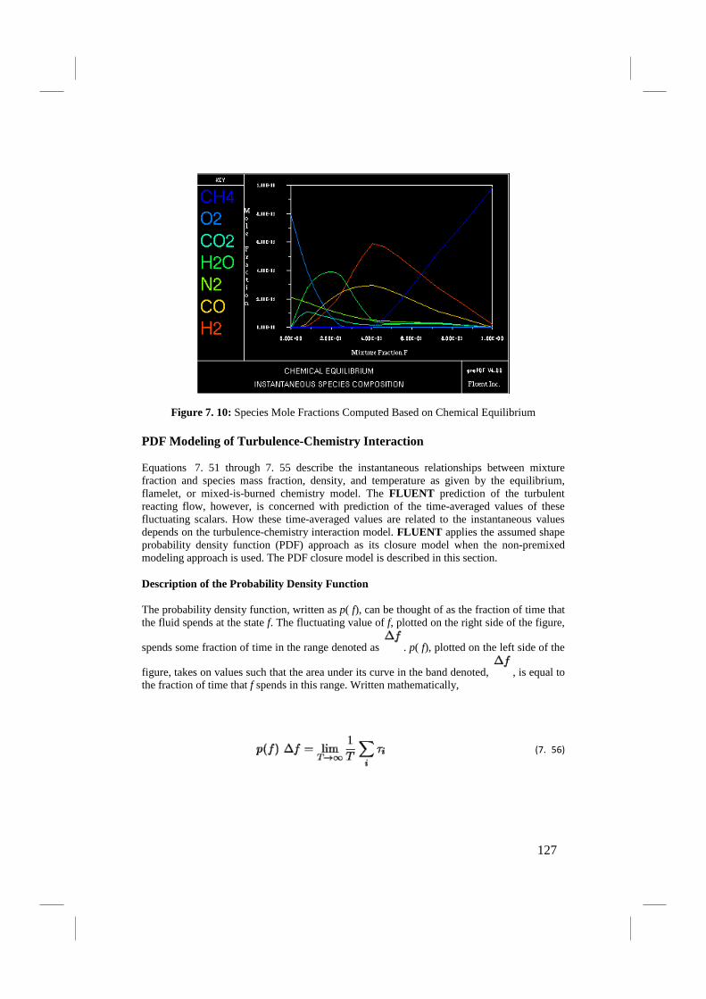
Figure 7. 10: Species Mole Fractions Computed Based on Chemical Equilibrium
PDF Modeling of Turbulence-Chemistry Interaction
Equations 7. 51 through 7. 55 describe the instantaneous relationships between mixture fraction and species mass fraction, density, and temperature as given by the equilibrium, flamelet, or mixed-is-burned chemistry model. The FLUENT prediction of the turbulent reacting flow, however, is concerned with prediction of the time-averaged values of these fluctuating scalars. How these time-averaged values are related to the instantaneous values depends on the turbulence-chemistry interaction model. FLUENT applies the assumed shape probability density function (PDF) approach as its closure model when the non-premixed modeling approach is used. The PDF closure model is described in this section.
Description of the Probability Density Function
The probability density function, written as p( f), can be thought of as the fraction of time that the fluid spends at the state f. The fluctuating value of f, plotted on the right side of the figure,
spends some fraction of time in the range denoted as . p( f), plotted on the left side of the
figure, takes on values such that the area under its curve in the band denoted, , is equal to the fraction of time that f spends in this range. Written mathematically,
(7. 56)
127

where T is the time scale and is the amount of time that f spends in the band. The shape of the function p( f) depends on the nature of the turbulent fluctuations in f. In practice, p( f) is expressed as a mathematical function that approximates the PDF shapes that have been observed experimentally.
Figure 7. 11:
Derivation of Mean Scalar Values from the Instantaneous Mixture Fraction
Graphical Description of the Probability Density Function, p( f)
The probability density function p( f), describing the temporal fluctuations of f in the turbulent flow, has the very beneficial property that it can be used to compute time-averaged values of variables that depend on f. Time-averaged values of species mole fractions and temperature can be computed (in adiabatic systems) as
(7. 57)
for a single mixture fraction system. When a secondary stream exists, the average values are calculated as
(7. 58)
128
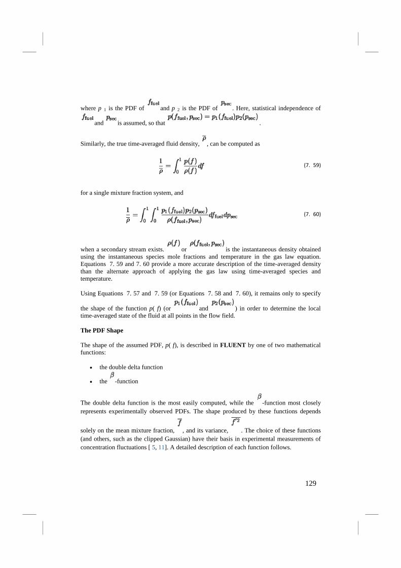
where p 1 is the PDF of and p 2 is the PDF of . Here, statistical independence of
and is assumed, so that .
Similarly, the true time-averaged fluid density, , can be computed as
(7. 59)
for a single mixture fraction system, and
(7. 60)
when a secondary stream exists. or is the instantaneous density obtained using the instantaneous species mole fractions and temperature in the gas law equation. Equations 7. 59 and 7. 60 provide a more accurate description of the time-averaged density than the alternate approach of applying the gas law using time-averaged species and temperature.
Using Equations 7. 57 and 7. 59 (or Equations 7. 58 and 7. 60), it remains only to specify
the shape of the function p( f) (or and ) in order to determine the local time-averaged state of the fluid at all points in the flow field.
The PDF Shape
The shape of the assumed PDF, p( f), is described in FLUENT by one of two mathematical functions:
• the double delta function
• the -function
The double delta function is the most easily computed, while the -function most closely represents experimentally observed PDFs. The shape produced by these functions depends
solely on the mean mixture fraction, , and its variance, . The choice of these functions (and others, such as the clipped Gaussian) have their basis in experimental measurements of concentration fluctuations [ 5, 11]. A detailed description of each function follows.
129
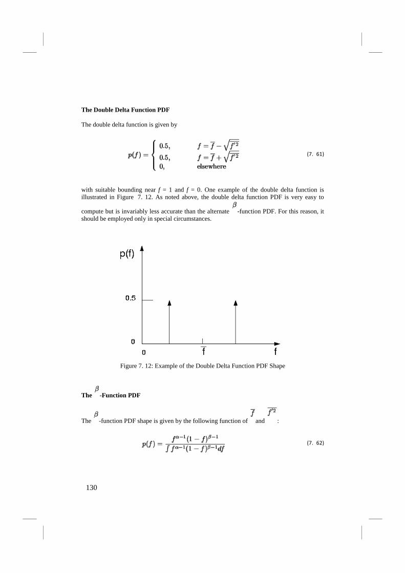
The Double Delta Function PDF
The double delta function is given by
(7. 61)
with suitable bounding near f = 1 and f = 0. One example of the double delta function is illustrated in Figure 7. 12. As noted above, the double delta function PDF is very easy to
compute but is invariably less accurate than the alternate -function PDF. For this reason, it should be employed only in special circumstances.
Figure 7. 12:
The
Example of the Double Delta Function PDF Shape
-Function PDF
The -function PDF shape is given by the following function of and :
(7. 62)
130

where
(7. 63)
and
(7. 64)
Figures 7. 13 and 7. 14 show the form of the function for two conditions of and .
Figure 7. 13: -Function PDF Shapes for = 0.3 and = 0.005
131
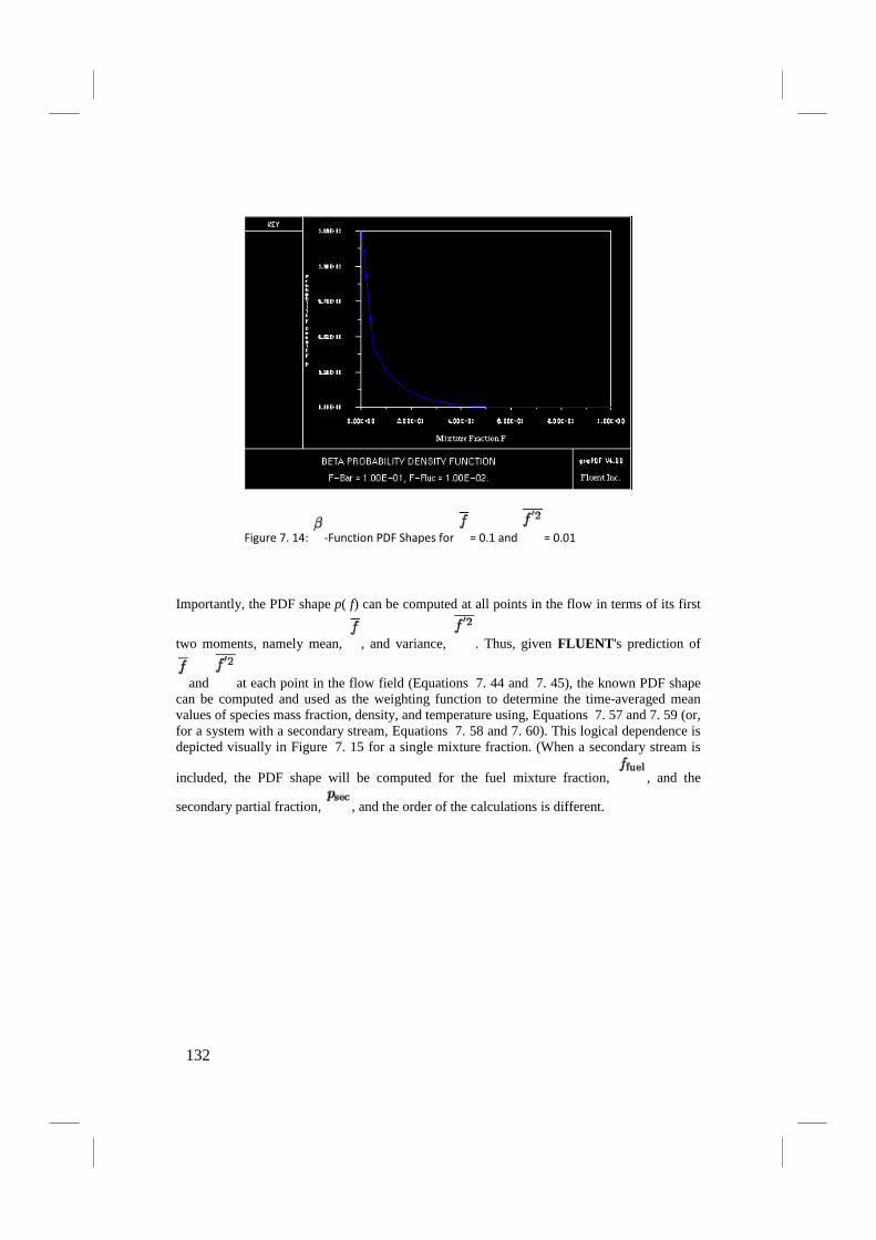
Figure 7. 14: -Function PDF Shapes for = 0.1 and = 0.01
Importantly, the PDF shape p( f) can be computed at all points in the flow in terms of its first
two moments, namely mean, , and variance, . Thus, given FLUENT's prediction of
and at each point in the flow field (Equations 7. 44 and 7. 45), the known PDF shape can be computed and used as the weighting function to determine the time-averaged mean values of species mass fraction, density, and temperature using, Equations 7. 57 and 7. 59 (or, for a system with a secondary stream, Equations 7. 58 and 7. 60). This logical dependence is depicted visually in Figure 7. 15 for a single mixture fraction. (When a secondary stream is
included, the PDF shape will be computed for the fuel mixture fraction, , and the
secondary partial fraction, , and the order of the calculations is different.
132
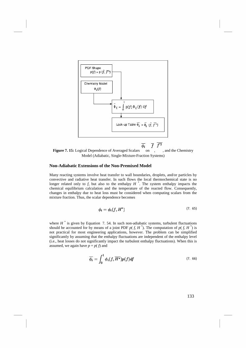
Figure 7. 15: Logical Dependence of Averaged Scalars on , , and the Chemistry Model (Adiabatic, Single-Mixture-Fraction Systems)
Non-Adiabatic Extensions of the Non-Premixed Model
Many reacting systems involve heat transfer to wall boundaries, droplets, and/or particles by convective and radiative heat transfer. In such flows the local thermochemical state is no longer related only to f, but also to the enthalpy H
*. The system enthalpy impacts the chemical equilibrium calculation and the temperature of the reacted flow. Consequently, changes in enthalpy due to heat loss must be considered when computing scalars from the mixture fraction. Thus, the scalar dependence becomes
(7. 65)
where H * is given by Equation 7. 54. In such non-adiabatic systems, turbulent fluctuations should be accounted for by means of a joint PDF p( f, H *). The computation of p( f, H *) is not practical for most engineering applications, however. The problem can be simplified significantly by assuming that the enthalpy fluctuations are independent of the enthalpy level (i.e., heat losses do not significantly impact the turbulent enthalpy fluctuations). When this is assumed, we again have p = p( f) and
(7. 66)
133
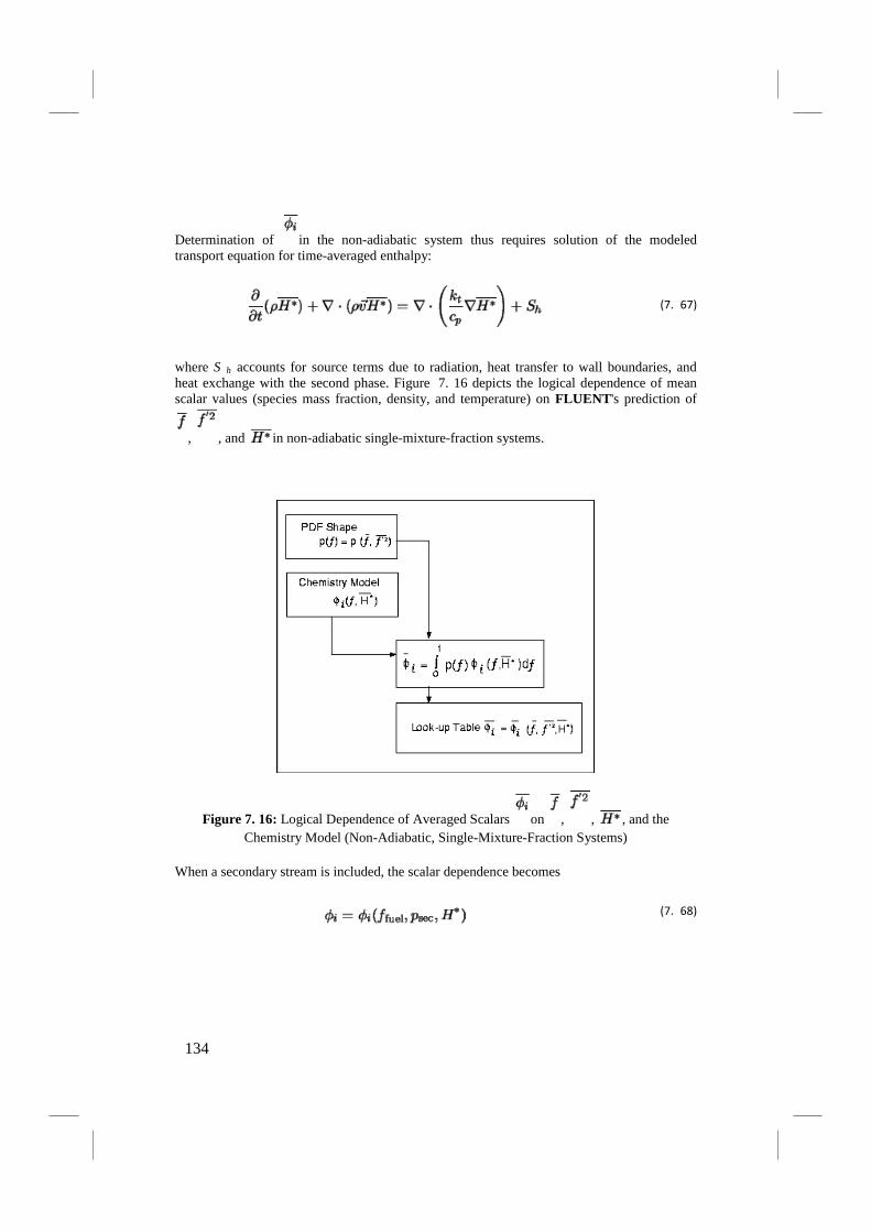
Determination of in the non-adiabatic system thus requires solution of the modeled transport equation for time-averaged enthalpy:
(7. 67)
where S h accounts for source terms due to radiation, heat transfer to wall boundaries, and heat exchange with the second phase. Figure 7. 16 depicts the logical dependence of mean scalar values (species mass fraction, density, and temperature) on FLUENT's prediction of
, , and in non-adiabatic single-mixture-fraction systems.
Figure 7. 16: Logical Dependence of Averaged Scalars on , , , and the Chemistry Model (Non-Adiabatic, Single-Mixture-Fraction Systems)
When a secondary stream is included, the scalar dependence becomes
(7. 68)
134

and the mean values are calculated from
(7. 69)
As noted above, the non-adiabatic extensions to the PDF model are required in systems involving heat transfer to walls and in systems with radiation included. In addition, the non-adiabatic model is required in systems that include multiple fuel or oxidizer inlets with different inlet temperatures or that include flue gas recycle. Finally, the non-adiabatic model is required in particle-laden flows (e.g., liquid fuel systems or coal combustion systems) since such flows include heat transfer to the dispersed phase. Figure 7. 16 illustrates several systems that must include the non-adiabatic form of the PDF model. Note that even if your system is non-adiabatic, you may want to perform the much simpler adiabatic calculation as an initial exercise. This will allow you to bound the non-adiabatic analysis in an efficient manner.
135

Figure 7. 17:
Reacting Systems Requiring Non-Adiabatic Non-Premixed Model Approach
136

7.5.4. Restrictions and Special Cases for the Non-Premixed Model
Restrictions on the Mixture Fraction Approach
The unique dependence of
(species mass fractions, density, or temperature) on f (Equation 7. 51 or 7. 52) requires that the reacting system meet the following conditions:
• The chemical system must be of the diffusion type with discrete fuel and oxidizer inlets (spray combustion and pulverized fuel flames may also fall into this category).
• The Lewis number must be unity. (This implies that the diffusion coefficients for all species and enthalpy are equal, a good approximation in turbulent flow).
• When a single mixture fraction is used, the following conditions must be met: o Only one type of fuel is involved. The fuel may be made up of a burnt mixture
of reacting species (e.g., 90% CH 4 and 10% CO) and you may include multiple fuel inlets. The multiple fuel inlets must have the same composition, however. Two or more fuel inlets with different fuel composition are not allowed (e.g., one inlet of CH 4
o Only one type of oxidizer is involved. The oxidizer may consist of a mixture of species (e.g., 21% O
and one inlet of CO). Similarly, in spray combustion systems or in systems involving reacting particles, only one off-gas is permitted.
2 and 79% N 2
• When two mixture fractions are used, three streams can be involved in the system. Valid systems are as follows:
) and you may have multiple oxidizer inlets. The multiple oxidizer inlets must, however, have the same composition. Two or more oxidizer inlets with different composition are not allowed (e.g., one inlet of air and a second inlet of pure oxygen).
o Two fuel streams with different compositions and one oxidizer stream. Each fuel stream may be made up of a mixture of reacting species (e.g., 90% CH 4 and 10% CO). You may include multiple inlets of each fuel stream, but each fuel inlet must have one of the two defined compositions (e.g., one inlet of CH 4
o Mixed fuel systems including gas-liquid, gas-coal, or liquid-coal fuel mixtures with a single oxidizer. In systems with a gas-coal or liquid-coal fuel mixture, the coal volatiles and char are treated as a single composite fuel stream.
and one inlet of CO).
o Coal combustion in which volatiles and char are tracked separately. o Two oxidizer streams with different compositions and one fuel stream. Each
oxidizer stream may consist of a mixture of species (e.g. 21% O 2 and 79% N 2
o A fuel stream, an oxidizer stream, and a non-reacting secondary stream.
). You may have multiple inlets of each oxidizer stream, but each oxidizer inlet must have one of the two defined compositions (e.g., one inlet of air and a second inlet of pure oxygen).
• The flow must be turbulent.
It is important to emphasize that these restrictions eliminate the use of the non-premixed approach for directly modeling premixed combustion. This is because the unburned premixed stream is far from chemical equilibrium.
137
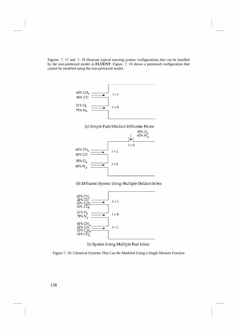
Figures 7. 17 and 7. 18 illustrate typical reacting system configurations that can be handled by the non-premixed model in FLUENT. Figure 7. 19 shows a premixed configuration that cannot be modeled using the non-premixed model.
Figure 7. 18:
Chemical Systems That Can Be Modeled Using a Single Mixture Fraction
138
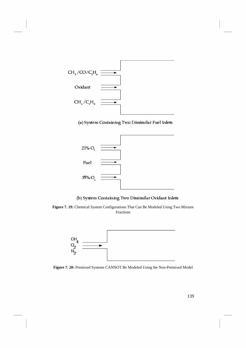
Figure 7. 19:
Chemical System Configurations That Can Be Modeled Using Two Mixture Fractions
Figure 7. 20: Premixed Systems CANNOT Be Modeled Using the Non-Premixed Model
139
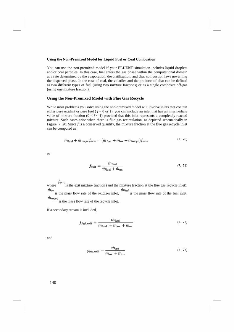
Using the Non-Premixed Model for Liquid Fuel or Coal Combustion
You can use the non-premixed model if your FLUENT simulation includes liquid droplets and/or coal particles. In this case, fuel enters the gas phase within the computational domain at a rate determined by the evaporation, devolatilization, and char combustion laws governing the dispersed phase. In the case of coal, the volatiles and the products of char can be defined as two different types of fuel (using two mixture fractions) or as a single composite off-gas (using one mixture fraction).
Using the Non-Premixed Model with Flue Gas Recycle
While most problems you solve using the non-premixed model will involve inlets that contain either pure oxidant or pure fuel ( f = 0 or 1), you can include an inlet that has an intermediate value of mixture fraction (0 < f < 1) provided that this inlet represents a completely reacted mixture. Such cases arise when there is flue gas recirculation, as depicted schematically in Figure 7. 20. Since f is a conserved quantity, the mixture fraction at the flue gas recycle inlet can be computed as
(7. 70)
or
(7. 71)
where is the exit mixture fraction (and the mixture fraction at the flue gas recycle inlet),
is the mass flow rate of the oxidizer inlet, is the mass flow rate of the fuel inlet,
is the mass flow rate of the recycle inlet.
If a secondary stream is included,
(7. 72)
and
(7. 73)
140
7.5.5. Modeling Approaches for Non-Premixed Equilibrium Chemistry
The FLUENT software package offers two different ways to model non-premixed equilibrium chemistry. You can choose either a single- or two-mixture-fraction approach depending on how many streams you have. prePDF stores information about the streams in ``look-up tables'', which are then used by FLUENT to solve for the mixture fraction, enthalpy, and scalar quantities.
7.5.5.1. Single-Mixture-Fraction Approach
To keep computation time to a minimum, much of the calculation required for the non-premixed model is performed outside of the FLUENT simulation by preprocessing the chemistry calculations and PDF integrations in a separate code, called prePDF. Figure 7. 21 illustrates how the computational effort is divided between the preprocessor ( prePDF) and the solver ( FLUENT). In prePDF, the chemistry model (mixed-is-burned, equilibrium chemistry, or laminar flamelet) is used in conjunction with the assumed shape of the PDF to perform the integrations given in Equations 7. 57, 7. 59, and/or 7. 66. These integrations are performed within prePDF and stored in look-up tables that relate the mean thermochemical
variables (temperature, density and species mass fractions) to the values of , , and
. Note that the scaled mixture fraction variance is used for tabulation, where is defined as
(7. 74)
Equations 7.44, 7. 45, and 7. 67 (for non-adiabatic systems) are solved in FLUENT to
obtain local values of , , and .
141
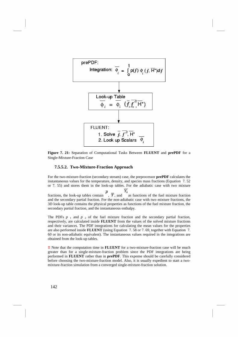
Figure 7. 21:
7.5.5.2. Two-Mixture-Fraction Approach
Separation of Computational Tasks Between FLUENT and prePDF for a Single-Mixture-Fraction Case
For the two-mixture-fraction (secondary stream) case, the preprocessor prePDF calculates the instantaneous values for the temperature, density, and species mass fractions (Equation 7. 52 or 7. 55) and stores them in the look-up tables. For the adiabatic case with two mixture
fractions, the look-up tables contain , , and as functions of the fuel mixture fraction and the secondary partial fraction. For the non-adiabatic case with two mixture fractions, the 3D look-up table contains the physical properties as functions of the fuel mixture fraction, the secondary partial fraction, and the instantaneous enthalpy.
The PDFs p 1 and p 2
!! Note that the computation time in FLUENT for a two-mixture-fraction case will be much greater than for a single-mixture-fraction problem since the PDF integrations are being performed in FLUENT rather than in prePDF. This expense should be carefully considered before choosing the two-mixture-fraction model. Also, it is usually expedient to start a two-mixture-fraction simulation from a converged single-mixture-fraction solution.
of the fuel mixture fraction and the secondary partial fraction, respectively, are calculated inside FLUENT from the values of the solved mixture fractions and their variances. The PDF integrations for calculating the mean values for the properties are also performed inside FLUENT (using Equation 7. 58 or 7. 69, together with Equation 7. 60 or its non-adiabatic equivalent). The instantaneous values required in the integrations are obtained from the look-up tables.
142

Figure 7. 22 illustrates the division of labor between prePDF and FLUENT for the two-mixture-fraction case.
Figure 7. 22:
Separation of Computational Tasks Between FLUENT and prePDF for a Two-Mixture-Fraction Case
7.5.5.2.1. The Look-Up Table Concept
Look-Up Tables for Adiabatic Systems
Figure
7. 23 illustrates the concept of the look-up tables generated by prePDF for a single-
mixture-fraction system. Given FLUENT's predicted value for and at a point in the
flow domain, the time-averaged mean value of mass fractions, density, or temperature ( ) at that point can be obtained from the table. FLUENT first uses Equation 7. 61 to compute
the scaled mixture fraction variance because the single-mixture-fraction look-up tables
contain property data as a function of and , rather than and .
The table, Figure 7. 23, is the mathematical result of the integration of Equation 7. 57. There is one look-up table of this type for each scalar of interest (species mass fractions, density, temperature). In adiabatic systems, where the instantaneous enthalpy is a function only of the
143

instantaneous mixture fraction, a two-dimensional look-up table, like that in Figure 7. 23, is all that is required.
Figure 7. 23: Visual Representation of a Look-Up Table for the Scalar as a Function of
and in Adiabatic Single-Mixture-Fraction Systems
For a system with two mixture fractions, there will be a look-up table for each instantaneous
scalar property as a function of the fuel mixture fraction and the secondary partial
fraction (Equation 7. 52), as shown in Figure 7. 24.
Figure 7. 24: Visual Representation of a Look-Up Table for the Scalar as a Function of
and in Adiabatic Two-Mixture-Fraction Systems.
144
3D Look-Up Tables for Non-Adiabatic Systems
In non-adiabatic systems, where the enthalpy is not linearly related to the mixture fraction, but depends also on wall heat transfer and/or radiation, a look-up table is required for each possible enthalpy value in the system. The result is a three-dimensional look-up table, as illustrated in Figure 7. 25, which consists of layers of two-dimensional tables, each one corresponding to the normalized heat loss or gain. The first layer or slice corresponds to the maximum heat loss for the system, where all the points in the look-up table are at the minimum temperature defined in the problem setup. The maximum slice corresponds to the heat gain that occurs when all points have reached the maximum temperature defined. The zero heat loss/gain slice corresponds to adiabatic operation. Slices interpolated between the adiabatic and maximum slices correspond to heat gain, and those interpolated between the adiabatic and minimum slices correspond to heat loss.
The three-dimensional look-up table allows FLUENT to determine the value of each mass
fraction, density, and temperature from calculated values of , , and . This three-dimensional table is the visual representation of the integral in Equation 7. 66.
145
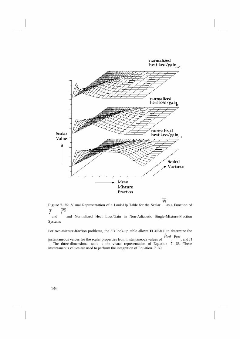
Figure 7. 25: Visual Representation of a Look-Up Table for the Scalar as a Function of
and and Normalized Heat Loss/Gain in Non-Adiabatic Single-Mixture-Fraction Systems
For two-mixture-fraction problems, the 3D look-up table allows FLUENT to determine the
instantaneous values for the scalar properties from instantaneous values of , , and H *
. The three-dimensional table is the visual representation of Equation 7. 68. These instantaneous values are used to perform the integration of Equation 7. 69.
146

Figure 7. 26: Visual Representation of a Look-Up Table for the Scalar as a Function of
, , and Normalized Heat Loss/Gain in Non-Adiabatic Two-Mixture-Fraction Systems
See Table 7. 2 for a summary of the look-up table structure.
Summary of Look-Up Table Formats
Table 7. 2 summarizes the look-up table format for different types of non-premixed models.
147

Table 7. 2: Look-Up Table Formats
Type of Model Adiabatic Non-Adiabatic
single mixture fraction
, , ,
two mixture fractions , , , H *
7.6. Modeling Liquid Fuel Combustion Using the Non-Premixed
Model
Liquid fuel combustion can be modeled with the non-premixed model. In prePDF, the fuel vapor, which is produced by evaporation of the liquid fuel, is defined as the fuel stream, and the oxidizer (e.g., air) inlet composition is defined as the oxidizer stream. The liquid fuel that evaporates within the domain appears as a source of the fuel mixture fraction, f, when the non-premixed model is used.
Within FLUENT, you define the liquid fuel model in the usual way. The gas phase (oxidizer) flow inlet is modeled using an inlet mixture fraction of zero and the fuel droplets are introduced as discrete-phase injections. The property inputs for the liquid fuel droplets are unaltered by the non-premixed model, and should be input as usual. Note that when you are requested to input the gas phase species destination for the evaporating liquid, you should input the species that comprises the fuel stream as defined in prePDF.
Note that if the fuel stream was defined as a mixture of components in prePDF, you should simply select one of these components as the ``evaporating species''. FLUENT will ensure that the mass evaporated from the liquid droplet enters the gas phase as a source of the fuel mixture that you defined in prePDF. The evaporating species you select here is used only to compute the diffusion controlled driving force in the evaporation rate.
7.6.1. Adding New Species to the prePDF Database
prePDF uses the CHEMKIN database [ 112], THERMO.DB, for species thermodynamic properties (see [ 12] for information on the parameters and the format required for the THERMO.DB file). If you wish to add a new species, you will need to add the thermodynamic data to the THERMO.DB file, as well as to the corresponding FLUENT database file, named thermodb.scm
You can use prePDF to generate the required
.
thermodb.scm file:
148
1.
Calculate the PDF look-up table in prePDF with the new species and the new THERMO.DB
2.
database file.
Generate a FLUENT property file with a default name prepdf.scm
File
.
Write Thermodb...
3.
You now have two choices:
• Rename prepdf.scm to thermodb.scm, and run FLUENT from the local directory where thermodb.scm
• If you would like to store the new species permanently, edit the file is.
thermodb.scm
path
in the
/Fluent.Inc/fluent6.x/cortex/lib/
installation directory (where path is the directory in which you have installed FLUENT and the variable x corresponds to your release version, e.g.,
0 for fluent6.0) and add in the new species from prepdf.scm. Be careful to keep the Scheme lists, enclosed within round parentheses, intact, and also ensure that your editor does not insert carriage-returns to break up the inserted Scheme lists. It is recommended that you save a backup copy of thermodb.scm
before making any changes.
149
Bibliography [1] Ansys. www.ansys.com 2006. [2] Atkins WS., Consultants and Members of the NSC, Best Practice Guidelines for Marine
Aplications of Computational Fluid Dynamics, Sirehna, HSVA, FLOWTECH, VTT, Imperial College of Science & Technology, Germanischer Lloyd, Astilleros Espanoles, http://pronet.wsatkins.co.uk/marnet/
[3] A. A. Amsden. KIVA-3: A KIVA Program with Block-Structured Mesh for Complex Geometries. Technical Report LA-12503-MS, UC-361, Los Alamos National Laboratory, Los Alamos, New Mexico, March 1993.
[4] T. B. Anderson and R. Jackson. A Fluid Mechanical Description of Fluidized Beds. I & EC Fundam., 6:527{534, 1967.
[5] J. Baldyga. Turbulent mixer model with application to homogenous instantaneous chemical reactions. Chem. Eng. Sci., 44:1175{1182, 1989.
[6] J. Blauvens, B. Smets, and J. Peters. In 16th Symp. (Int'l.) on Combustion. The Combustion Institute, 1977.
[7] K. S. Brentner and F. Farassat. An Analytical Comparison of the Acoustic Analogy and Kirchhoff Formulations for Moving Surfaces. AIAA Journal, 36(8), 1998.
[8] S. Brunauer. The Absorption of Gases and Vapors. Princeton University Press, Princeton, NJ, 1943.
[9] P. R. Desam. Subgrid Scale Model Development and Validation for Thermal Nitric Oxide Prediction in Glass Furnaces. PhD thesis, The University of Utah, 2005.
[10] N. Dombrowski and W. R. Johns. The aerodynamic Instability and Disintegration of Viscous Liquid Sheets. Chemical Engineering Science, 18:203, 1963.
[11] J. E. Ffowcs-Williams and D. L. Hawkings. Sound Generation by Turbulence and Surfaces in Arbitrary Motion. Proc. Roy. Soc. London, A264:3{342, 1969.
[12] W. L. Flower, R. K. Hanson, and C. H. Kruger. In 15th Symp. (Int'l.) on Combustion, page 823. The Combustion Institute, 1975.
[13] Fluent Inc., Fluent 6.1 User`s Guide, 2003. [14] Fluent Inc., Fluent 6.3 User`s Guide, 2008. [15] M. Germano, U. Piomelli, P. Moin, and W. H. Cabot. Dynamic Subgrid-Scale Eddy
Viscosity Model. In Summer Workshop, Center for Turbulence Research, Stanford, CA, 1996.
[16] D. Gidaspow. Multiphase Flow and Fluidization. Academic Press, Boston, 1994. [17] D. M. Grant, R. J. Pugmire, T. H. Fletcher, and A. R. Kerstein. Chemical percolation
model of coal devolatilization using percolation lattice statistics. Energy and Fuels, 3:175, 1989.
[18] Gryboś R., Podstawy Mechaniki Płynów, Wydawnictwo Naukowe PWN, Warszawa, 1998.
[19] A. Haider and O. Levenspiel. Drag Coe_cient and Terminal Velocity of Spherical and Nonspherical Particles. Powder Technology, 58:63{70, 1989.
[20] R. K. Hanson and S. Salimian. Survey of Rate Constants in H/N/O Systems. In W. C. Gardiner, editor, Combustion Chemistry, page 361, 1984.
[21] R. A. W. M. Henkes, F. F. van der Flugt, and C. J. Hoogendoorn. Natural Convection Flow in a Square Cavity Calculated with Low-Reynolds-Number Turbulence Models. Int. J. Heat Mass Transfer, 34:1543{1557, 1991.
[22] K. Hsu and A. Jemcov. Numerical investigation of detonation in premixed hydrogen-air mixture - assessment of simpli_ed chemical mechanisms. Technical Report AIAA-
150

2000-2478, American Institute of Aeronautics and Astronautics, Fluids 2000 Conference and Exhibit, Denver, CO, June 2000.
[23] P. Huang, P. Bradshaw, and T. Coakley. Skin Friction and Velocity Profile Family for Compressible Turbulent Boundary Layers. AIAA Journal, 31(9):1600{1604, September 1993.
[24] M. E. Larsen and J. R. Howell. Least Squares Smoothing of Direct Exchange Areas in Zonal Analysis. J. Heat Transfer, 108:239{242, 1986.
[25] M. J. Lighthill. On Sound Generated Aerodynamically. Proc. Roy. Soc. London, A211:564{587, 1952.
[26] D. Ma and G. Ahmadi. A Thermodynamical Formulation for Dispersed Multiphase Turbulent Flows. Int. J. Multiphase Flow, 16:323{351, 1990.
[27] M. Manninen, V. Taivassalo, and S. Kallio. On the mixture model for multiphase flow. VTT Publications 288, Technical Research Centre of Finland, 1996.
[28] M. J. Moran and H. N. Shapiro. Fundamentals of Engineering Thermodynamics. John Wiley & Sons, Inc, 1988.
[29] R. Ocone, S. Sundaresan, and R. Jackson. Gas-particle ow in a duct of arbitrary inclination with particle-particle interaction. AIChE J., 39:1261{1271, 1993.
[30] Johnson R., Fluid Dynamice, CRC Press LLC, Floryda, 1998. [31] Rusiński E, Czmochowski J, Smolnicki T, Zaawansowana metoda elementów
skończonych w konstrukcjach nośnych, Oficyna Wydawnicza Politechniki Wrocławskiej, Wrocław, 2000.
[32] G. G. De Soete. Overall Reaction Rates of NO and N2 Formation from Fuel Nitrogen. In 15th Symp. (Int'l.) on Combustion, pages 1093{1102. The Combustion Institute, 1975.
[33] Zienkiewicz O., Metoda Elementów Skończonych, Arkady, Warszawa, 1972.
151