What common factors are driving inflation in CEE countries? · Grzegorz Szafrański –...
38
NBP Working Paper No. 225 What common factors are driving inflation in CEE countries? Aleksandra Hałka, Grzegorz Szafrański
Transcript of What common factors are driving inflation in CEE countries? · Grzegorz Szafrański –...
NBP Working Paper No. 225
What common factors are driving inflation in CEE countries?
Aleksandra Hałka, Grzegorz Szafrański
Economic InstituteWarsaw, 2015
NBP Working Paper No. 225
What common factors are driving inflation in CEE countries?
Aleksandra Hałka, Grzegorz Szafrański
Published by: Narodowy Bank Polski Education & Publishing Department ul. Świętokrzyska 11/21 00-919 Warszawa, Poland phone +48 22 185 23 35 www.nbp.pl
ISSN 2084-624X
© Copyright Narodowy Bank Polski, 2015
Aleksandra Hałka – Narodowy Bank Polski; [email protected] Szafrański – Corresponding author: Grzegorz Szafrański, Narodowy Bank Polski,
and Univeristy of Lodz, The Faculty of Economics and Sociology, Department of Econometrics; [email protected]
The views expressed herein are those of the authors and not necessarily of the institutions they represent. The authors wish to thank the participants of the NBP seminar, 13th EBES Conference, SSEM EuroConference 2014, the Conference on Advances in Applied Macro-Finance and Forecasting in 2014, and AAMFF2014 Conference whose invaluable feedback we benefited from in the course of our research.
3NBP Working Paper No. 225
Contents1 Introduction 5
2. The Hierarchical Model 10
3. Data 15
4. Results 18
Factor decomposition 19CEE region-wide factors 23Country specific factors 25Sector specific factors 26
5. Conclusions 28
References 30
Appendix 1 Decomposition results of the base case with two aggregate factors 33
Appendix 2 Robustness analysis 35
Narodowy Bank Polski4
Abstract
3
Abstract
In this paper, we analyse the sources of time variation in consumer inflation across ten Central and Eastern European (CEE) countries and five sectors (durables, semi-durables, non-durables, food, and services) in the period 2001-2013. With a multi-level factor model we decompose product-level HICP inflation rates into the following components: CEE region wide, sector, country, country-sector, and idiosyncratic. The outcomes indicate that region-wide and country specific components of inflation are more persistent than sector and product-level components, which is in line with similar studies for core EU countries. Two region-wide factors explain about 17% of variance in monthly price changes, whereas the other common components explain below 10% each. The results are at odds with empirical evidence on the importance of sectoral price shocks in developed economies and the volatility-persistence puzzle. This difference may be related to the conclusion that the first region-wide factor is associated with common disinflationary processes that occurred in CEE economies in 2000s, whereas the second one reveals significant correlations with global factors, especially commodity prices and euro area price developments. JEL: C38, C55, E31, E52, F62 Keywords: product-level inflation, CEE economies, multi-level factor model
4
1. Introduction
The literature of the past two decades suggests that there is a high degree of
comovement in inflation rates across countries. One of the popular explanation of this
stylized fact is a globalization effect, which is responsible for weakening of the
relationship between inflation and domestic economic activity (Borio and Filardo,
2007). In consequence, a growing synchronization of price changes is observed among
the countries which are strongly connected in terms of trade and financial market.
With the increased economic openness the vulnerability to common external shocks,
coming from commodity prices (including oil), exchange rates, stock prices or interest
rates on sovereign debt also increases. The literature that deals with these issues
usually analyses inflation at the aggregate level. Ciccarelli and Mojon (2010) find that
nearly 70% of inflation volatility in 22 developed OECD countries in the period 1960-
2008 is driven by a global factor. Hence, they claim that inflation is a global
phenomenon. Hakkio (2009) examines various inflation measures for the OECD
countries and states that “the commonality of (…) inflation rates reflects the
commonality of the determinants of inflation”. Beck et al. (2006) conduct similar
analysis at the regional level in euro area countries. They conclude that common euro
area and country specific factors are explaining a substantial part of inflation with
idiosyncratic regional variability playing a minor role.
There is also a strand of literature on price determination, which attempts to reconcile
high persistence of inflation observed at the aggregate level with microeconomic
evidence suggesting that sectoral and individual prices are transient and volatile (see
Bils and Klenow, 2004 for micro-evidence). This is a volatility-persistence inflation
puzzle which is at odds with microeconomic foundations of many sectoral New-
Keynesian DSGE models (see discussion in Maćkowiak, Moench and Wiederholt,
5NBP Working Paper No. 225
Chapter 1
3
Abstract
In this paper, we analyse the sources of time variation in consumer inflation across ten Central and Eastern European (CEE) countries and five sectors (durables, semi-durables, non-durables, food, and services) in the period 2001-2013. With a multi-level factor model we decompose product-level HICP inflation rates into the following components: CEE region wide, sector, country, country-sector, and idiosyncratic. The outcomes indicate that region-wide and country specific components of inflation are more persistent than sector and product-level components, which is in line with similar studies for core EU countries. Two region-wide factors explain about 17% of variance in monthly price changes, whereas the other common components explain below 10% each. The results are at odds with empirical evidence on the importance of sectoral price shocks in developed economies and the volatility-persistence puzzle. This difference may be related to the conclusion that the first region-wide factor is associated with common disinflationary processes that occurred in CEE economies in 2000s, whereas the second one reveals significant correlations with global factors, especially commodity prices and euro area price developments. JEL: C38, C55, E31, E52, F62 Keywords: product-level inflation, CEE economies, multi-level factor model
4
1. Introduction
The literature of the past two decades suggests that there is a high degree of
comovement in inflation rates across countries. One of the popular explanation of this
stylized fact is a globalization effect, which is responsible for weakening of the
relationship between inflation and domestic economic activity (Borio and Filardo,
2007). In consequence, a growing synchronization of price changes is observed among
the countries which are strongly connected in terms of trade and financial market.
With the increased economic openness the vulnerability to common external shocks,
coming from commodity prices (including oil), exchange rates, stock prices or interest
rates on sovereign debt also increases. The literature that deals with these issues
usually analyses inflation at the aggregate level. Ciccarelli and Mojon (2010) find that
nearly 70% of inflation volatility in 22 developed OECD countries in the period 1960-
2008 is driven by a global factor. Hence, they claim that inflation is a global
phenomenon. Hakkio (2009) examines various inflation measures for the OECD
countries and states that “the commonality of (…) inflation rates reflects the
commonality of the determinants of inflation”. Beck et al. (2006) conduct similar
analysis at the regional level in euro area countries. They conclude that common euro
area and country specific factors are explaining a substantial part of inflation with
idiosyncratic regional variability playing a minor role.
There is also a strand of literature on price determination, which attempts to reconcile
high persistence of inflation observed at the aggregate level with microeconomic
evidence suggesting that sectoral and individual prices are transient and volatile (see
Bils and Klenow, 2004 for micro-evidence). This is a volatility-persistence inflation
puzzle which is at odds with microeconomic foundations of many sectoral New-
Keynesian DSGE models (see discussion in Maćkowiak, Moench and Wiederholt,
Narodowy Bank Polski6
5
2009). The potential explanation of the puzzle1 is provided by Maćkowiak and
Wiederholt (2009) in a rational inattention model. In this model representative firms
being under information processing constraints rationally allocate more attention to
idiosyncratic shocks than to aggregate ones, which are usually less volatile and more
persistent. Boivin, Giannoni and Mihov (2009) claim that distinguishing between sector
specific and aggregate sources of price fluctuations is a key point in understanding the
volatility-persistence puzzle.
Most of the inflation decomposition studies relies on a static representation of dynamic
factor model (e.g. Ciccarelli and Mojon, 2010, Boivin et al., 2006, and Maćkowiak et al.
2009). With such an approach idiosyncratic residuals may capture sector, geographical,
country specific components and also other measurement errors. To handle this
problem some authors use two-level factor model to decompose inflation into common
(global) and sector or geographical factors at different levels of aggregation (e.g.
Krusper, 2012, or Altissimo et al., 2011). Multi-level factor models are becoming more
and more popular in the literature. Starting with the study of Kose, Otrok and
Whiteman (2003) on commonality of business cycles new estimation methods in a
dynamic factor setup have been proposed like sequential least squares and canonical
correlation analysis (see Breitung and Eickmeier, 2014), with Bayesian analysis at the
front (Moench, Ng and Potter, 2013). A comprehensive approach for decomposition in
a multi-level factor model with an overlapping data blocks, we use, is the one
proposed by Beck et al. (2011).
We argue that CEE countries on their road to the European Union have experienced
similar inflationary pressures of economic (common market) and political origin
(nominal convergence criteria). They all have experienced an economic transformation
in the period of 1990s and they are strongly linked to the EU common market, which
1 Other popular explanations are aggregation bias or structural break in the mean of inflation during the sample period (see Beck et al., 2011).
6
makes us believe that they share some similarities in price dynamics not only at the
regional level, but also at the sectoral level. Nowadays these small open economies are
still converging with an objective to join euro area in a far or near future or they have
joined EMU already.2 In spite of some differences between CEE countries in terms of
trade openness, economic structures, exchange rate regimes etc. we provide evidence
that there are common components in inflation dynamics across countries and sectors.
The existence of, both, global and domestic common factors driving inflation in CEE
countries has already been advocated by several authors (e.g. Maćkowiak, 2006;
Stavrev, 2009; Krusper, 2012; Alexova, 2012). Most of these studies analyse inflation at
the aggregate level, without looking deeper into the sectoral determinants of price
changes. We claim that in some sectors there are similar vulnerabilities to market
integration and globalization effects. In other sectors there are possibly relevant
differences stemming from institutional matters like price-setting behaviours
(including the scope of market and price administration).
The empirical research on commonality in disaggregated inflation rates is scarce.
Monacelli and Sala (2009) looks for the contribution of the international components
that are responsible for the product-level inflation in 4 major OECD countries. Choueiri
et al. (2008) analyses disaggregated CPI indices for 25 countries of the European Union.
With the exception of Stavrev (2009) the other studies of sectoral or product-level price
changes usually deal with price comovements in the developed countries like US
(Boivin et al., 2009; Maćkowiak et al., 2009) or the euro area (Beck et al., 2011;
Kaufmann and Lein 2013). Interestingly, when analysing disaggregated price indices
common factors become less important than in the case of the aggregate analysis (cf.
Boivin et al., 2009, Beck et al., 2011).
2 See article of Staehr (2010) on divergent patterns of EMU entrance across countries.
7NBP Working Paper No. 225
Introduction
5
2009). The potential explanation of the puzzle1 is provided by Maćkowiak and
Wiederholt (2009) in a rational inattention model. In this model representative firms
being under information processing constraints rationally allocate more attention to
idiosyncratic shocks than to aggregate ones, which are usually less volatile and more
persistent. Boivin, Giannoni and Mihov (2009) claim that distinguishing between sector
specific and aggregate sources of price fluctuations is a key point in understanding the
volatility-persistence puzzle.
Most of the inflation decomposition studies relies on a static representation of dynamic
factor model (e.g. Ciccarelli and Mojon, 2010, Boivin et al., 2006, and Maćkowiak et al.
2009). With such an approach idiosyncratic residuals may capture sector, geographical,
country specific components and also other measurement errors. To handle this
problem some authors use two-level factor model to decompose inflation into common
(global) and sector or geographical factors at different levels of aggregation (e.g.
Krusper, 2012, or Altissimo et al., 2011). Multi-level factor models are becoming more
and more popular in the literature. Starting with the study of Kose, Otrok and
Whiteman (2003) on commonality of business cycles new estimation methods in a
dynamic factor setup have been proposed like sequential least squares and canonical
correlation analysis (see Breitung and Eickmeier, 2014), with Bayesian analysis at the
front (Moench, Ng and Potter, 2013). A comprehensive approach for decomposition in
a multi-level factor model with an overlapping data blocks, we use, is the one
proposed by Beck et al. (2011).
We argue that CEE countries on their road to the European Union have experienced
similar inflationary pressures of economic (common market) and political origin
(nominal convergence criteria). They all have experienced an economic transformation
in the period of 1990s and they are strongly linked to the EU common market, which
1 Other popular explanations are aggregation bias or structural break in the mean of inflation during the sample period (see Beck et al., 2011).
6
makes us believe that they share some similarities in price dynamics not only at the
regional level, but also at the sectoral level. Nowadays these small open economies are
still converging with an objective to join euro area in a far or near future or they have
joined EMU already.2 In spite of some differences between CEE countries in terms of
trade openness, economic structures, exchange rate regimes etc. we provide evidence
that there are common components in inflation dynamics across countries and sectors.
The existence of, both, global and domestic common factors driving inflation in CEE
countries has already been advocated by several authors (e.g. Maćkowiak, 2006;
Stavrev, 2009; Krusper, 2012; Alexova, 2012). Most of these studies analyse inflation at
the aggregate level, without looking deeper into the sectoral determinants of price
changes. We claim that in some sectors there are similar vulnerabilities to market
integration and globalization effects. In other sectors there are possibly relevant
differences stemming from institutional matters like price-setting behaviours
(including the scope of market and price administration).
The empirical research on commonality in disaggregated inflation rates is scarce.
Monacelli and Sala (2009) looks for the contribution of the international components
that are responsible for the product-level inflation in 4 major OECD countries. Choueiri
et al. (2008) analyses disaggregated CPI indices for 25 countries of the European Union.
With the exception of Stavrev (2009) the other studies of sectoral or product-level price
changes usually deal with price comovements in the developed countries like US
(Boivin et al., 2009; Maćkowiak et al., 2009) or the euro area (Beck et al., 2011;
Kaufmann and Lein 2013). Interestingly, when analysing disaggregated price indices
common factors become less important than in the case of the aggregate analysis (cf.
Boivin et al., 2009, Beck et al., 2011).
2 See article of Staehr (2010) on divergent patterns of EMU entrance across countries.
Narodowy Bank Polski8
7
In the paper we decompose COICOP product-level HICP inflation rates of ten CEE
countries into aggregate, country, sector and country-sector specific common
components, and into idiosyncratic components. We also document the volatility-
persistence puzzle in components of HICP and provide economic discussion on the
possible sources of comovements among them. The novel contribution of our approach
to the analysis of sectoral inflation rates relies also in a unique product-level
decomposition. Our method is related to iterative non-parametric PCA-based method
of Beck et al. (2011), as we decompose common factors from overlapping data blocks,
but with a different hierarchical structure of the factor model.
From our decomposition we find that all common factors explain about 36.5% of
monthly inflation at a product level. Among them the most important are two CEE
region-wide factors that contribute to about half of the total variance explained (17%).
Regional component is very persistent, which is generally in line with similar studies
for core EU countries, but the degree of persistence is more than 3 times bigger than in
core EU or in OECD countries. Sectoral components (i.e. sector specific and country-
sector specific) are on average less persistent than macroeconomic components (i.e.
country and CEE region-wide) and as volatile as the latter. The results partly support
the view that firms, when setting the price, pay attention to both macroeconomic and
sectoral factors, although macroeconomic ones seem to be relatively more important in
CEE countries than in developed ones.
The second aim of our research is the interpretation of the forces behind unobserved
common factors. The outcomes indicate that the first CEE region-wide factor is
associated with disinflationary processes in CEE countries, whereas the second
regional factor reveals correlations with global factors, especially commodity prices
and euro area price developments. Euro-area and U.S business cycle conditions are
related to the country specific factors in Bulgaria, three Baltic countries and Poland. As
8
the sector specific factors are concerned, prices of food and other non-durable goods
strongly depend on the commodity markets. Prices of services reveal the moderate
correlation with unemployment. Surprisingly, there is hardly no influence of the
changes in the global or domestic economic activity on the prices of durable and semi-
durable goods. One of the possible explanation is the globalization effect, which leads
to price decreases regardless of the phase of the business cycle.
9NBP Working Paper No. 225
Introduction
7
In the paper we decompose COICOP product-level HICP inflation rates of ten CEE
countries into aggregate, country, sector and country-sector specific common
components, and into idiosyncratic components. We also document the volatility-
persistence puzzle in components of HICP and provide economic discussion on the
possible sources of comovements among them. The novel contribution of our approach
to the analysis of sectoral inflation rates relies also in a unique product-level
decomposition. Our method is related to iterative non-parametric PCA-based method
of Beck et al. (2011), as we decompose common factors from overlapping data blocks,
but with a different hierarchical structure of the factor model.
From our decomposition we find that all common factors explain about 36.5% of
monthly inflation at a product level. Among them the most important are two CEE
region-wide factors that contribute to about half of the total variance explained (17%).
Regional component is very persistent, which is generally in line with similar studies
for core EU countries, but the degree of persistence is more than 3 times bigger than in
core EU or in OECD countries. Sectoral components (i.e. sector specific and country-
sector specific) are on average less persistent than macroeconomic components (i.e.
country and CEE region-wide) and as volatile as the latter. The results partly support
the view that firms, when setting the price, pay attention to both macroeconomic and
sectoral factors, although macroeconomic ones seem to be relatively more important in
CEE countries than in developed ones.
The second aim of our research is the interpretation of the forces behind unobserved
common factors. The outcomes indicate that the first CEE region-wide factor is
associated with disinflationary processes in CEE countries, whereas the second
regional factor reveals correlations with global factors, especially commodity prices
and euro area price developments. Euro-area and U.S business cycle conditions are
related to the country specific factors in Bulgaria, three Baltic countries and Poland. As
8
the sector specific factors are concerned, prices of food and other non-durable goods
strongly depend on the commodity markets. Prices of services reveal the moderate
correlation with unemployment. Surprisingly, there is hardly no influence of the
changes in the global or domestic economic activity on the prices of durable and semi-
durable goods. One of the possible explanation is the globalization effect, which leads
to price decreases regardless of the phase of the business cycle.
Narodowy Bank Polski10
Chapter 2
9
2. The Hierarchical Model
In most of the studies, in which global components of inflation are extracted (Ciccarelli
and Mojon, 2010) or the aggregation volatility-persistence puzzle is documented
(Boivin et al. 2009), the decomposition of inflation to sectoral and global components is
based on a simple framework of a first-order factor model. The simple specification is
suitable to introduce the dynamic relationship between common factors and
observables (like in a FAVAR approach by Monacelli and Sala, 2009), but it has a major
drawback. It implicitly assumes no hierarchical structure in the data in terms of
commonalities within a country or inside a sector. Hence, in this type of factor analyses
common sources of variability originating from sector or country specific factors are
not properly treated leaving interpretations of idiosyncratic terms dubious.
The datasets with sectoral and geographical dimensions should be better analysed with
a higher order hierarchical unobserved common factor models. Simple second-order
factor models have been already used in the analyses of regional inflation rates – e.g.
Beck et al. (2006) and Krusper (2012) leading to the following decomposition of sectoral
inflation rates, , in a country and a region :
(1)
where represents global (aggregate) common factors,
– factors specific to a subset
of countries (e.g. CEE) or regions in a given country and is an idiosyncratic
white-noise component.
Different sets of dimensions { } in are applied in the literature depending on the
focus of the research and the data availability. For example, Krusper (2012) in a panel
of HICP inflation rates for EU27 is interested in a regional component of inflation for
10 CEE countries, hence he defines as a country, and as a region. In another second-
order factor study Beck et al. (2006) analyse regional overall HICP inflation rates in
NUTS region of EMU country .
10
As a multi-level factor model augments an original specification of an approximate
factor model by Stock and Watson (2002) a two-step method of principal components
(PC) is usually applied to estimate orthogonal factors common at an aggregate level
and factors common at a lower level of aggregation. In the first step orthogonal
aggregate common factors are extracted by PC and then they are used as regressors
to calculate OLS residuals ( ). In the second step, in order to
extract the lower-level common factors (), PC is run separately on a subset of
belonging to the group . Finally, to obtain estimates of factor loadings (
) and
idiosyncratic terms (), OLS regression of on a set of estimated factor scores
{ } is performed.
In our study we analyse sectoral COICOP product-level data on HICP inflation rates in
10 CEE countries. Although the data set in our study is also overlapping in terms of
sectoral and geographical (countries) dimensions, it is the sectoral (not geographical as
in Beck, et al. 2011) dimension which is defined at superior (5 broad groups: durables,
semi-durables, non-durables, food and services) and subordinate (mostly 4-digit
COICOP) level. Formally, we apply the following static representation of a multi-level
factor model offering the following economic interpretation for the common factors:
(2)
where:
are aggregate (regional CEE-wide) factors, which are common to all items () in a
dataset and which are potentially related to common EU trade policy, or other external
developments like shocks to commodity prices, global financial crisis,
are factors specific for sector (group of goods like durables, semi-durables, non-
durables, food, and services), which are potentially related to sectoral policy (e.g.
Common Agricultural Market), shocks in oil market, changes to consumption patterns,
11NBP Working Paper No. 225
The Hierarchical Model
9
2. The Hierarchical Model
In most of the studies, in which global components of inflation are extracted (Ciccarelli
and Mojon, 2010) or the aggregation volatility-persistence puzzle is documented
(Boivin et al. 2009), the decomposition of inflation to sectoral and global components is
based on a simple framework of a first-order factor model. The simple specification is
suitable to introduce the dynamic relationship between common factors and
observables (like in a FAVAR approach by Monacelli and Sala, 2009), but it has a major
drawback. It implicitly assumes no hierarchical structure in the data in terms of
commonalities within a country or inside a sector. Hence, in this type of factor analyses
common sources of variability originating from sector or country specific factors are
not properly treated leaving interpretations of idiosyncratic terms dubious.
The datasets with sectoral and geographical dimensions should be better analysed with
a higher order hierarchical unobserved common factor models. Simple second-order
factor models have been already used in the analyses of regional inflation rates – e.g.
Beck et al. (2006) and Krusper (2012) leading to the following decomposition of sectoral
inflation rates, , in a country and a region :
(1)
where represents global (aggregate) common factors,
– factors specific to a subset
of countries (e.g. CEE) or regions in a given country and is an idiosyncratic
white-noise component.
Different sets of dimensions { } in are applied in the literature depending on the
focus of the research and the data availability. For example, Krusper (2012) in a panel
of HICP inflation rates for EU27 is interested in a regional component of inflation for
10 CEE countries, hence he defines as a country, and as a region. In another second-
order factor study Beck et al. (2006) analyse regional overall HICP inflation rates in
NUTS region of EMU country .
10
As a multi-level factor model augments an original specification of an approximate
factor model by Stock and Watson (2002) a two-step method of principal components
(PC) is usually applied to estimate orthogonal factors common at an aggregate level
and factors common at a lower level of aggregation. In the first step orthogonal
aggregate common factors are extracted by PC and then they are used as regressors
to calculate OLS residuals ( ). In the second step, in order to
extract the lower-level common factors (), PC is run separately on a subset of
belonging to the group . Finally, to obtain estimates of factor loadings (
) and
idiosyncratic terms (), OLS regression of on a set of estimated factor scores
{ } is performed.
In our study we analyse sectoral COICOP product-level data on HICP inflation rates in
10 CEE countries. Although the data set in our study is also overlapping in terms of
sectoral and geographical (countries) dimensions, it is the sectoral (not geographical as
in Beck, et al. 2011) dimension which is defined at superior (5 broad groups: durables,
semi-durables, non-durables, food and services) and subordinate (mostly 4-digit
COICOP) level. Formally, we apply the following static representation of a multi-level
factor model offering the following economic interpretation for the common factors:
(2)
where:
are aggregate (regional CEE-wide) factors, which are common to all items () in a
dataset and which are potentially related to common EU trade policy, or other external
developments like shocks to commodity prices, global financial crisis,
are factors specific for sector (group of goods like durables, semi-durables, non-
durables, food, and services), which are potentially related to sectoral policy (e.g.
Common Agricultural Market), shocks in oil market, changes to consumption patterns,
Narodowy Bank Polski12
11
geographical proximity or differences in exchange rate pass-through effects on
tradables and non-tradables,
are country-specific factors representing such events in country economic policies
as VAT changes, currency depreciation, etc.,
are country and sector-specific factors that affect only prices in a sector in a
country (like energy prices in Poland, or food prices in Romania),
are respective factor loadings specific for each product-level item,
and represent idiosyncratic terms.
We identify orthogonal common factors from overlapping cross-sections (geographical
and sectoral) using disaggregated information. The novel contribution of our approach
to the analysis of sectoral and country inflation rates relies in a unique decomposition
of product-level HICPs. Another important distinction is an interpretation of sector-
specific factors at this level of inflation disaggregation. Firstly, our sectors are much
broadly defined than in other studies. Secondly, the information on the comovements
comes from the product-level HICP inflation rates. According to our knowledge this
level of disaggregation was not analysed with an overlapping third-order hierarchical
factor model until now.
In estimation we follow a non-parametric (based on principal components) method of
Beck et al. (2011), which in a multi-sequential iterative version is capable of treating the
overlapping data blocks in an appropriate way.3 Yet, we apply the estimation method
to a different dataset structure. To this extent an iterative estimation procedure has
been adapted which consists of the following steps. In the first step we estimate CEE
region-wide factors obtained from the whole data set by the method of principal 3 The small samples properties of this method were tested by the authors – see Monte Carlo experiments in Beck et al. (2011). Breitung and Eickmeier (2014) also find that under a relatively big importance of higher order factor (as in our case) two-step PC estimator delivers good efficiency when compared to its non-Bayesian competitors.
12
components (PC) and extract idiosyncratic components as the part of price variability
not explained by CEE region-wide factors (these are OLS residuals of regressing
on factors ). From these residuals (demeaned across countries) in the second step we
estimate sector-specific factors by PC method in each subset of sectoral data
separately.4 In the third step the OLS residuals from regressions of inflation rates on
the estimated CEE region-wide and sector-specific factors ( ) are used to
distinguish country-specific factors () in each country data subset separately. In the
final step one obtains country-sector specific factors () running PC on residuals from
the second step separately in each data subset of a given country in a given sector.
Finally, we also propose an extraction of common CEE region-wide components from
final residuals, separately for each COICOP category and give the discussion on their
interpretations.
The number of factors may be established by the cumulative percentage of variance
explained by factors or with more formal information criteria (Bai and Ng, 2002). The
decomposition of lower-order factors, however, is conditional on the number of factors
extracted at higher order level. Selecting more than one factor at each level also poses
serious identification problems. Usually the orthogonality condition is used but it is
not guaranteed by iterative procedure. As a result, the more of the higher level factors
one extracts, the less variability is left for explaining lower-level factors. Consequently,
the sequential top-down estimation method, as well as other competitors based on an
asymptotic inference (see Breitung and Eickmeier 2014), are more efficient in extracting
higher-order factors than lower-order ones. Thus, in the empirical part of the study we
select only one common factor for each lower-level factor and we perform sensitivity
4 The necessary modification in the iterative procedure compared to the two-step approach of Beck et al. (2011) is iteration between steps of obtaining different lower order factors. Our method is different in the second and the third step. Instead of country-specific factors we estimate sector-specific factors first. Because of relatively small number of items in overlapping country and sector cross-sections we repeat the lower-order factor extraction procedure (from step 2 to step 3) until convergence.
13NBP Working Paper No. 225
The Hierarchical Model
11
geographical proximity or differences in exchange rate pass-through effects on
tradables and non-tradables,
are country-specific factors representing such events in country economic policies
as VAT changes, currency depreciation, etc.,
are country and sector-specific factors that affect only prices in a sector in a
country (like energy prices in Poland, or food prices in Romania),
are respective factor loadings specific for each product-level item,
and represent idiosyncratic terms.
We identify orthogonal common factors from overlapping cross-sections (geographical
and sectoral) using disaggregated information. The novel contribution of our approach
to the analysis of sectoral and country inflation rates relies in a unique decomposition
of product-level HICPs. Another important distinction is an interpretation of sector-
specific factors at this level of inflation disaggregation. Firstly, our sectors are much
broadly defined than in other studies. Secondly, the information on the comovements
comes from the product-level HICP inflation rates. According to our knowledge this
level of disaggregation was not analysed with an overlapping third-order hierarchical
factor model until now.
In estimation we follow a non-parametric (based on principal components) method of
Beck et al. (2011), which in a multi-sequential iterative version is capable of treating the
overlapping data blocks in an appropriate way.3 Yet, we apply the estimation method
to a different dataset structure. To this extent an iterative estimation procedure has
been adapted which consists of the following steps. In the first step we estimate CEE
region-wide factors obtained from the whole data set by the method of principal 3 The small samples properties of this method were tested by the authors – see Monte Carlo experiments in Beck et al. (2011). Breitung and Eickmeier (2014) also find that under a relatively big importance of higher order factor (as in our case) two-step PC estimator delivers good efficiency when compared to its non-Bayesian competitors.
12
components (PC) and extract idiosyncratic components as the part of price variability
not explained by CEE region-wide factors (these are OLS residuals of regressing
on factors ). From these residuals (demeaned across countries) in the second step we
estimate sector-specific factors by PC method in each subset of sectoral data
separately.4 In the third step the OLS residuals from regressions of inflation rates on
the estimated CEE region-wide and sector-specific factors ( ) are used to
distinguish country-specific factors () in each country data subset separately. In the
final step one obtains country-sector specific factors () running PC on residuals from
the second step separately in each data subset of a given country in a given sector.
Finally, we also propose an extraction of common CEE region-wide components from
final residuals, separately for each COICOP category and give the discussion on their
interpretations.
The number of factors may be established by the cumulative percentage of variance
explained by factors or with more formal information criteria (Bai and Ng, 2002). The
decomposition of lower-order factors, however, is conditional on the number of factors
extracted at higher order level. Selecting more than one factor at each level also poses
serious identification problems. Usually the orthogonality condition is used but it is
not guaranteed by iterative procedure. As a result, the more of the higher level factors
one extracts, the less variability is left for explaining lower-level factors. Consequently,
the sequential top-down estimation method, as well as other competitors based on an
asymptotic inference (see Breitung and Eickmeier 2014), are more efficient in extracting
higher-order factors than lower-order ones. Thus, in the empirical part of the study we
select only one common factor for each lower-level factor and we perform sensitivity
4 The necessary modification in the iterative procedure compared to the two-step approach of Beck et al. (2011) is iteration between steps of obtaining different lower order factors. Our method is different in the second and the third step. Instead of country-specific factors we estimate sector-specific factors first. Because of relatively small number of items in overlapping country and sector cross-sections we repeat the lower-order factor extraction procedure (from step 2 to step 3) until convergence.

Narodowy Bank Polski14
13
analysis to the selection of the number of aggregate factors (see Appendix 2). The
possible correlation between extracted common factors may be also a good diagnostic
tool of estimation problems.
14
3. Data
We analyse components of monthly Harmonized Index of Consumer Prices (HICP)
from 10 Central and Eastern European (CEE) countries: Bulgaria (BL), Czech Republic
(CZ), Estonia (EE), Hungary (HU), Latvia (LV), Lithuania (LT), Poland (PL), Romania
(RO), Slovakia (SK) and Slovenia (SI) for the period Jan. 2001 - Sept. 2013. These are all
emerging market economies that have entered the EU in the sample period (BL, RO in
January 2007, the others in May 2004). The selection reflects the choice of many authors
interested in disentangling common- and country-specific factors across new EU
members (see Stavrev, 2009; Krusper, 2012).
To capture the co-movements in inflation rates across countries and sectors we employ
the price indices at the disaggregation level up to four COICOP (Classification of
Individual Consumption According to Purpose) digits, which we call, in short,
product-level data. When analysing sector-specific factors we group these HICP
components into 5 exclusive categories (named sectors for convenience). These are
services, food (which includes beverages, alcohol and tobacco), and three non-food
good categories: durables, semi-durables, non-durables. The distinction between semi-
durables and non-durables originates from Eurostat NACE Rev. 1 classification and is
defined by differences in a way (semi-)durable goods are used (‘repeatedly or
continuously over a period of time considerably more than one year’) and their
expected lifetime (for semi-durables it is shorter than for durables).
The original database consists of 94 product-level categories. There are a few categories
of the consumption basket with a missing values at the beginning of the sample due to
the late acquisition of good quality data. We omit some COICOP categories with
market prices observed only in a few of 10 CEE countries (like combined passenger
transport or maintenance and repair of other major durables for recreation and
culture). We also skip another 51 time series with zero monthly price changes in more
15NBP Working Paper No. 225
Chapter 3
13
analysis to the selection of the number of aggregate factors (see Appendix 2). The
possible correlation between extracted common factors may be also a good diagnostic
tool of estimation problems.
14
3. Data
We analyse components of monthly Harmonized Index of Consumer Prices (HICP)
from 10 Central and Eastern European (CEE) countries: Bulgaria (BL), Czech Republic
(CZ), Estonia (EE), Hungary (HU), Latvia (LV), Lithuania (LT), Poland (PL), Romania
(RO), Slovakia (SK) and Slovenia (SI) for the period Jan. 2001 - Sept. 2013. These are all
emerging market economies that have entered the EU in the sample period (BL, RO in
January 2007, the others in May 2004). The selection reflects the choice of many authors
interested in disentangling common- and country-specific factors across new EU
members (see Stavrev, 2009; Krusper, 2012).
To capture the co-movements in inflation rates across countries and sectors we employ
the price indices at the disaggregation level up to four COICOP (Classification of
Individual Consumption According to Purpose) digits, which we call, in short,
product-level data. When analysing sector-specific factors we group these HICP
components into 5 exclusive categories (named sectors for convenience). These are
services, food (which includes beverages, alcohol and tobacco), and three non-food
good categories: durables, semi-durables, non-durables. The distinction between semi-
durables and non-durables originates from Eurostat NACE Rev. 1 classification and is
defined by differences in a way (semi-)durable goods are used (‘repeatedly or
continuously over a period of time considerably more than one year’) and their
expected lifetime (for semi-durables it is shorter than for durables).
The original database consists of 94 product-level categories. There are a few categories
of the consumption basket with a missing values at the beginning of the sample due to
the late acquisition of good quality data. We omit some COICOP categories with
market prices observed only in a few of 10 CEE countries (like combined passenger
transport or maintenance and repair of other major durables for recreation and
culture). We also skip another 51 time series with zero monthly price changes in more
Narodowy Bank Polski16
15
than 25% of the sample periods. These are mainly administered prices, although
different item categories are referred under this name in different countries and across
time. The administered prices are fixed for a considerable period of time between price
decisions of country-specific regulator, hence they are not suitable for correlation
analysis. Finally, we employ a balanced panel of 776 HICP-component series (from 74
components in Estonia to 82 in the Czech Republic) over 154 consecutive months (see
Table 1). The selected product-level HICP components are seasonally adjusted (SA) by
a Tramo/Seats automatic procedures. We provide the results for month-over-month
(mom) COICOP indices as a base case and for year-over-year (yoy) data as the
robustness check (see Table 8, Appendix 2). Due to high kurtosis the data are corrected
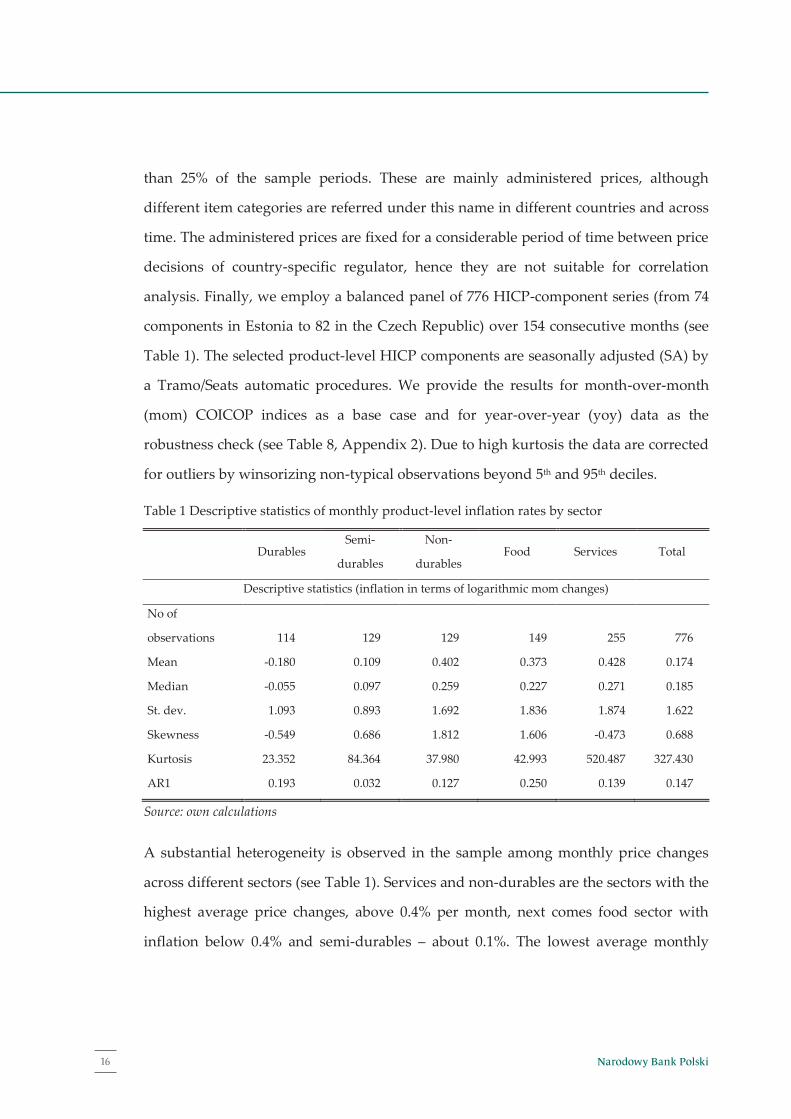
for outliers by winsorizing non-typical observations beyond 5th and 95th deciles.
Table 1 Descriptive statistics of monthly product-level inflation rates by sector
Durables
Semi-
durables
Non-
durables Food Services Total
Descriptive statistics (inflation in terms of logarithmic mom changes)
No of
observations 114 129 129 149 255 776
Mean -0.180 0.109 0.402 0.373 0.428 0.174
Median -0.055 0.097 0.259 0.227 0.271 0.185
St. dev. 1.093 0.893 1.692 1.836 1.874 1.622
Skewness -0.549 0.686 1.812 1.606 -0.473 0.688
Kurtosis 23.352 84.364 37.980 42.993 520.487 327.430
AR1 0.193 0.032 0.127 0.250 0.139 0.147
Source: own calculations
A substantial heterogeneity is observed in the sample among monthly price changes
across different sectors (see Table 1). Services and non-durables are the sectors with the
highest average price changes, above 0.4% per month, next comes food sector with
inflation below 0.4% and semi-durables – about 0.1%. The lowest average monthly
16
inflation is recorded for durables and it is negative (ca. -0.2%). This ordering of average
inflation rates from durables to non-durables is an interesting stylized fact in our
sample, however, its explanation is beyond the scope of our study. Unsurprisingly,
sectors with highest inflation are also those with highest price volatility (see Table 1).
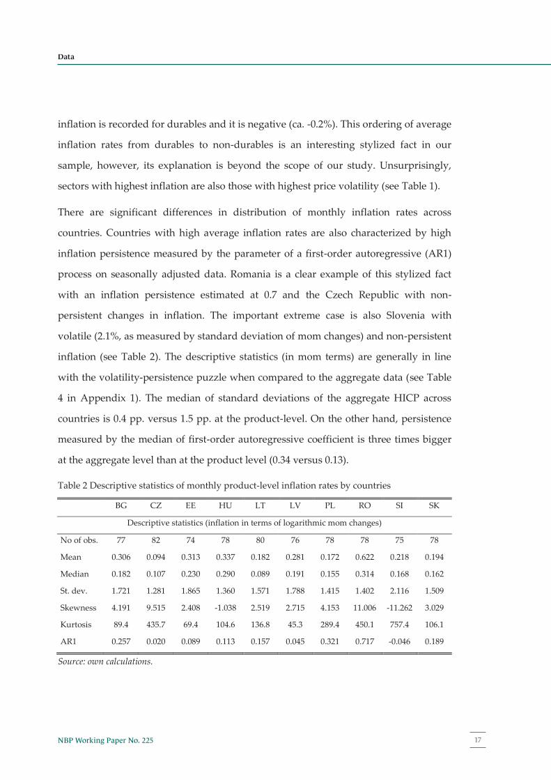
There are significant differences in distribution of monthly inflation rates across
countries. Countries with high average inflation rates are also characterized by high
inflation persistence measured by the parameter of a first-order autoregressive (AR1)
process on seasonally adjusted data. Romania is a clear example of this stylized fact
with an inflation persistence estimated at 0.7 and the Czech Republic with non-
persistent changes in inflation. The important extreme case is also Slovenia with
volatile (2.1%, as measured by standard deviation of mom changes) and non-persistent
inflation (see Table 2). The descriptive statistics (in mom terms) are generally in line
with the volatility-persistence puzzle when compared to the aggregate data (see Table
4 in Appendix 1). The median of standard deviations of the aggregate HICP across
countries is 0.4 pp. versus 1.5 pp. at the product-level. On the other hand, persistence
measured by the median of first-order autoregressive coefficient is three times bigger
at the aggregate level than at the product level (0.34 versus 0.13).
Table 2 Descriptive statistics of monthly product-level inflation rates by countries
BG CZ EE HU LT LV PL RO SI SK
Descriptive statistics (inflation in terms of logarithmic mom changes)
No of obs. 77 82 74 78 80 76 78 78 75 78
Mean 0.306 0.094 0.313 0.337 0.182 0.281 0.172 0.622 0.218 0.194
Median 0.182 0.107 0.230 0.290 0.089 0.191 0.155 0.314 0.168 0.162
St. dev. 1.721 1.281 1.865 1.360 1.571 1.788 1.415 1.402 2.116 1.509
Skewness 4.191 9.515 2.408 -1.038 2.519 2.715 4.153 11.006 -11.262 3.029
Kurtosis 89.4 435.7 69.4 104.6 136.8 45.3 289.4 450.1 757.4 106.1
AR1 0.257 0.020 0.089 0.113 0.157 0.045 0.321 0.717 -0.046 0.189
Source: own calculations.
17NBP Working Paper No. 225
Data
15
than 25% of the sample periods. These are mainly administered prices, although
different item categories are referred under this name in different countries and across
time. The administered prices are fixed for a considerable period of time between price
decisions of country-specific regulator, hence they are not suitable for correlation
analysis. Finally, we employ a balanced panel of 776 HICP-component series (from 74
components in Estonia to 82 in the Czech Republic) over 154 consecutive months (see
Table 1). The selected product-level HICP components are seasonally adjusted (SA) by
a Tramo/Seats automatic procedures. We provide the results for month-over-month
(mom) COICOP indices as a base case and for year-over-year (yoy) data as the
robustness check (see Table 8, Appendix 2). Due to high kurtosis the data are corrected
for outliers by winsorizing non-typical observations beyond 5th and 95th deciles.
Table 1 Descriptive statistics of monthly product-level inflation rates by sector
Durables
Semi-
durables
Non-
durables Food Services Total
Descriptive statistics (inflation in terms of logarithmic mom changes)
No of
observations 114 129 129 149 255 776
Mean -0.180 0.109 0.402 0.373 0.428 0.174
Median -0.055 0.097 0.259 0.227 0.271 0.185
St. dev. 1.093 0.893 1.692 1.836 1.874 1.622
Skewness -0.549 0.686 1.812 1.606 -0.473 0.688
Kurtosis 23.352 84.364 37.980 42.993 520.487 327.430
AR1 0.193 0.032 0.127 0.250 0.139 0.147
Source: own calculations
A substantial heterogeneity is observed in the sample among monthly price changes
across different sectors (see Table 1). Services and non-durables are the sectors with the
highest average price changes, above 0.4% per month, next comes food sector with
inflation below 0.4% and semi-durables – about 0.1%. The lowest average monthly
16
inflation is recorded for durables and it is negative (ca. -0.2%). This ordering of average
inflation rates from durables to non-durables is an interesting stylized fact in our
sample, however, its explanation is beyond the scope of our study. Unsurprisingly,
sectors with highest inflation are also those with highest price volatility (see Table 1).
There are significant differences in distribution of monthly inflation rates across
countries. Countries with high average inflation rates are also characterized by high
inflation persistence measured by the parameter of a first-order autoregressive (AR1)
process on seasonally adjusted data. Romania is a clear example of this stylized fact
with an inflation persistence estimated at 0.7 and the Czech Republic with non-
persistent changes in inflation. The important extreme case is also Slovenia with
volatile (2.1%, as measured by standard deviation of mom changes) and non-persistent
inflation (see Table 2). The descriptive statistics (in mom terms) are generally in line
with the volatility-persistence puzzle when compared to the aggregate data (see Table
4 in Appendix 1). The median of standard deviations of the aggregate HICP across
countries is 0.4 pp. versus 1.5 pp. at the product-level. On the other hand, persistence
measured by the median of first-order autoregressive coefficient is three times bigger
at the aggregate level than at the product level (0.34 versus 0.13).
Table 2 Descriptive statistics of monthly product-level inflation rates by countries
BG CZ EE HU LT LV PL RO SI SK
Descriptive statistics (inflation in terms of logarithmic mom changes)
No of obs. 77 82 74 78 80 76 78 78 75 78
Mean 0.306 0.094 0.313 0.337 0.182 0.281 0.172 0.622 0.218 0.194
Median 0.182 0.107 0.230 0.290 0.089 0.191 0.155 0.314 0.168 0.162
St. dev. 1.721 1.281 1.865 1.360 1.571 1.788 1.415 1.402 2.116 1.509
Skewness 4.191 9.515 2.408 -1.038 2.519 2.715 4.153 11.006 -11.262 3.029
Kurtosis 89.4 435.7 69.4 104.6 136.8 45.3 289.4 450.1 757.4 106.1
AR1 0.257 0.020 0.089 0.113 0.157 0.045 0.321 0.717 -0.046 0.189
Source: own calculations.
Narodowy Bank Polski18
Chapter 4
17
4. Results
In this section we present the empirical results with a disclaimer that they are
conditional on, both, the factor model structure and the estimation method applied.5
The results are presented for two CEE-wide regional factors (base case) which are
selected after the analysis of dominating eigenvalues on the scree plot (see Figure 3 in
Appendix 2). The lower-order factor decomposition (by sectors and countries) is
conditional on the selection of aggregate factors and on the cross-sectional breakdown
of the dataset.6 As a robustness check we briefly discuss differences to the
decomposition with three aggregate factors (see Table 7 in Appendix 2) and the
decomposition of year-over-year price indices (Table 8 in Appendix 2).
We start with a common factor decomposition to describe the fraction of variance
explained by common components, their volatility (in terms of standard deviation),
and persistence (first order autoregressive coefficient) in the full dataset. Then we
present similar decomposition at country and sectoral breakdown to point out some
important differences in subsamples. Next, we perform a correlation analysis of
aggregate factors. The last part of this section offers a preliminary analysis of sector-
specific components at the product level.
5 Particularly, the decomposition of unobserved factors and loadings at the upper (aggregate) level depends on usual PC restrictions (e.g. orthonormal factors), which are hard to be justified on economic grounds. Although there is a rotational indeterminacy of common factors (i.e. factors are identified up to a rotation by a non-singular matrix), PC-based decomposition is unique in terms of common and idiosyncratic components as long as the number of factors is known or fixed with some statistical criteria (see Bai, Ng 2013). Therefore, we do not interpret aggregate factors and their loadings separately, except for a preliminary correlation analysis. 6 Nevertheless, sector, country, and country-sector specific single factors are identified up to a sign and variance (a local identification). The iterative estimation procedure guarantees that the ordering of lower level factors does not influence the decomposition.
18
Factor decomposition
In this part we are interested in a decomposition of product-level inflation rates
according to a multi-level factor model (2). We name the decomposition with two
aggregate factors obtained with PC iterative method described in Section 3 as the base
case. The summary results are presented in Figure 1 and Table 3. The first aggregate
factor explains 10.8% of variation in prices at the product level, whereas the second one
explains 6.5%7. If we select the decomposition with three aggregate factors instead of
two, the contribution of country and country-sector specific components (altogether)
diminishes by 4 pp.8 The contribution of CEE region-wide component varies
considerably between different countries and sectors. It is the most prominent factor in
Romania (explaining 55% of price variability), and the least important for Estonia
(10%), the Czech Republic (8%) and Slovenia (6%). For the other countries the fraction
of explained variance is between 13% (Poland) and 18% (Bulgaria). The CEE region-
wide component explains from 11% of variance in food and non-durable sector to 24%
in services being the most important price determinant in each of them (c.f. Table 5 and
Table 6 in Appendix 1).
7 With each consecutive aggregate factors ordered by eigenvalues of correlation matrix the explained part would be lower than 3% which is below the fraction of variance explained by sector-specific factors (3.1%) if two aggregate factors are assumed. See Figure 3 in Appendix 2. 8 With the base case country specific and country-sector specific components explain, respectively, 6.5% and 9.6% of overall time variation in a panel, and in the three aggregate components 4.1% and 8.0% respectively.
19NBP Working Paper No. 225
Results
17
4. Results
In this section we present the empirical results with a disclaimer that they are
conditional on, both, the factor model structure and the estimation method applied.5
The results are presented for two CEE-wide regional factors (base case) which are
selected after the analysis of dominating eigenvalues on the scree plot (see Figure 3 in
Appendix 2). The lower-order factor decomposition (by sectors and countries) is
conditional on the selection of aggregate factors and on the cross-sectional breakdown
of the dataset.6 As a robustness check we briefly discuss differences to the
decomposition with three aggregate factors (see Table 7 in Appendix 2) and the
decomposition of year-over-year price indices (Table 8 in Appendix 2).
We start with a common factor decomposition to describe the fraction of variance
explained by common components, their volatility (in terms of standard deviation),
and persistence (first order autoregressive coefficient) in the full dataset. Then we
present similar decomposition at country and sectoral breakdown to point out some
important differences in subsamples. Next, we perform a correlation analysis of
aggregate factors. The last part of this section offers a preliminary analysis of sector-
specific components at the product level.
5 Particularly, the decomposition of unobserved factors and loadings at the upper (aggregate) level depends on usual PC restrictions (e.g. orthonormal factors), which are hard to be justified on economic grounds. Although there is a rotational indeterminacy of common factors (i.e. factors are identified up to a rotation by a non-singular matrix), PC-based decomposition is unique in terms of common and idiosyncratic components as long as the number of factors is known or fixed with some statistical criteria (see Bai, Ng 2013). Therefore, we do not interpret aggregate factors and their loadings separately, except for a preliminary correlation analysis. 6 Nevertheless, sector, country, and country-sector specific single factors are identified up to a sign and variance (a local identification). The iterative estimation procedure guarantees that the ordering of lower level factors does not influence the decomposition.
18
Factor decomposition
In this part we are interested in a decomposition of product-level inflation rates
according to a multi-level factor model (2). We name the decomposition with two
aggregate factors obtained with PC iterative method described in Section 3 as the base
case. The summary results are presented in Figure 1 and Table 3. The first aggregate
factor explains 10.8% of variation in prices at the product level, whereas the second one
explains 6.5%7. If we select the decomposition with three aggregate factors instead of
two, the contribution of country and country-sector specific components (altogether)
diminishes by 4 pp.8 The contribution of CEE region-wide component varies
considerably between different countries and sectors. It is the most prominent factor in
Romania (explaining 55% of price variability), and the least important for Estonia
(10%), the Czech Republic (8%) and Slovenia (6%). For the other countries the fraction
of explained variance is between 13% (Poland) and 18% (Bulgaria). The CEE region-
wide component explains from 11% of variance in food and non-durable sector to 24%
in services being the most important price determinant in each of them (c.f. Table 5 and
Table 6 in Appendix 1).
7 With each consecutive aggregate factors ordered by eigenvalues of correlation matrix the explained part would be lower than 3% which is below the fraction of variance explained by sector-specific factors (3.1%) if two aggregate factors are assumed. See Figure 3 in Appendix 2. 8 With the base case country specific and country-sector specific components explain, respectively, 6.5% and 9.6% of overall time variation in a panel, and in the three aggregate components 4.1% and 8.0% respectively.
Narodowy Bank Polski20
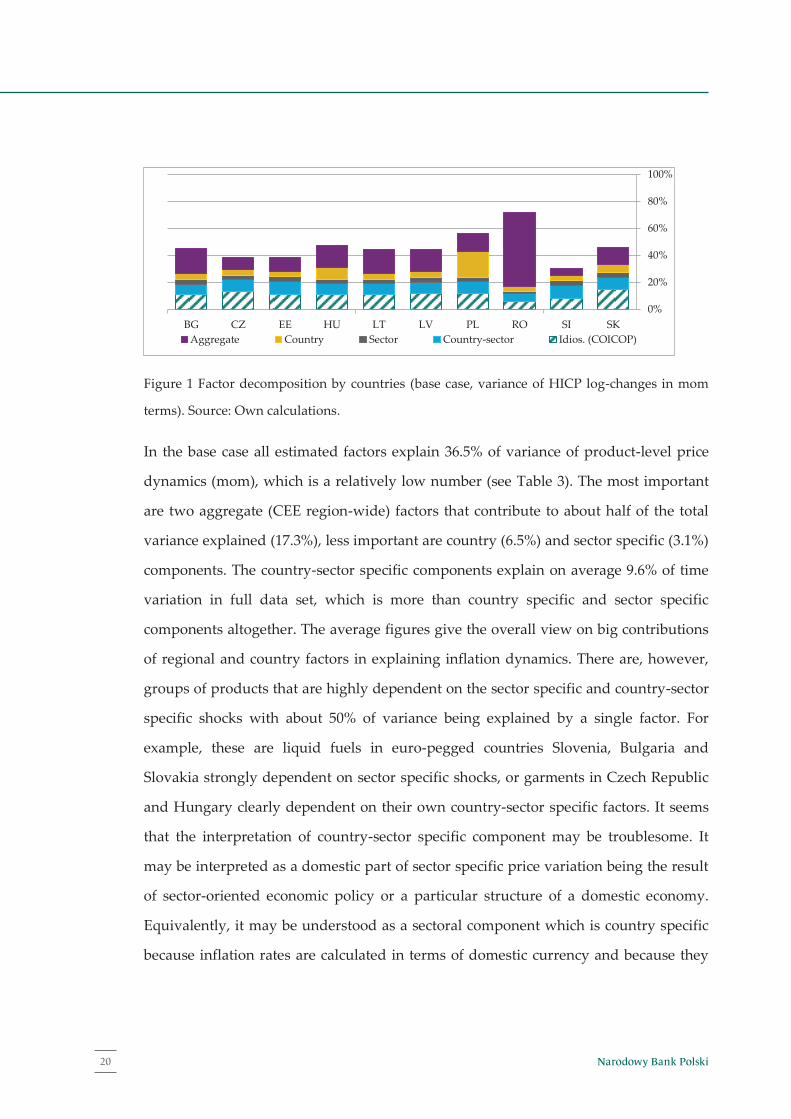
19
Figure 1 Factor decomposition by countries (base case, variance of HICP log-changes in mom
terms). Source: Own calculations.
In the base case all estimated factors explain 36.5% of variance of product-level price
dynamics (mom), which is a relatively low number (see Table 3). The most important
are two aggregate (CEE region-wide) factors that contribute to about half of the total
variance explained (17.3%), less important are country (6.5%) and sector specific (3.1%)
components. The country-sector specific components explain on average 9.6% of time
variation in full data set, which is more than country specific and sector specific
components altogether. The average figures give the overall view on big contributions
of regional and country factors in explaining inflation dynamics. There are, however,
groups of products that are highly dependent on the sector specific and country-sector
specific shocks with about 50% of variance being explained by a single factor. For
example, these are liquid fuels in euro-pegged countries Slovenia, Bulgaria and
Slovakia strongly dependent on sector specific shocks, or garments in Czech Republic
and Hungary clearly dependent on their own country-sector specific factors. It seems
that the interpretation of country-sector specific component may be troublesome. It
may be interpreted as a domestic part of sector specific price variation being the result
of sector-oriented economic policy or a particular structure of a domestic economy.
Equivalently, it may be understood as a sectoral component which is country specific
because inflation rates are calculated in terms of domestic currency and because they
0%
20%
40%
60%
80%
100%
BG CZ EE HU LT LV PL RO SI SKAggregate Country Sector Country-sector Idios. (COICOP)
20
are under the influence of country–wide regulations (like fiscal policy). We will follow
the second interpretation calling sector and country-sector specific components as the
components of sectoral origin. Following this interpretation the overall contribution of
sectoral factors is 13% on average, which is lower than the contribution of CEE region-
wide factors, but it is still a considerable explained part of mom inflation rates.
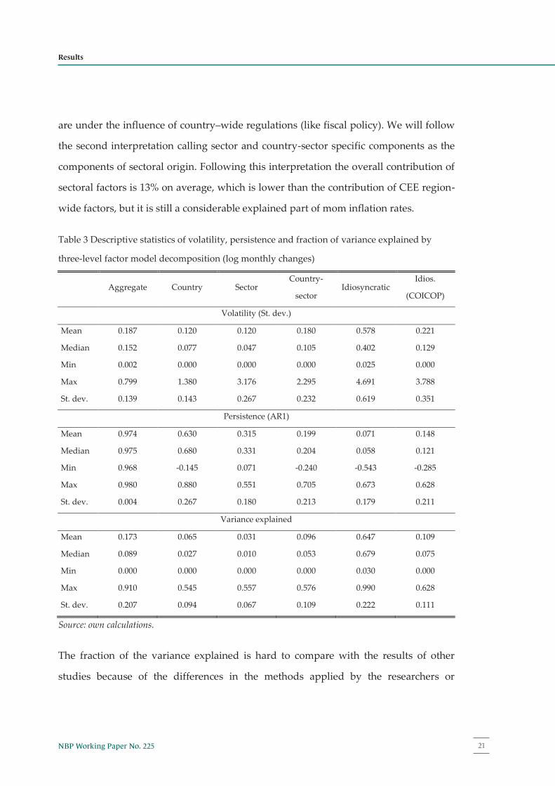
Table 3 Descriptive statistics of volatility, persistence and fraction of variance explained by
three-level factor model decomposition (log monthly changes)
Aggregate Country Sector Country-
sector Idiosyncratic
Idios.
(COICOP)
Volatility (St. dev.)
Mean 0.187 0.120 0.120 0.180 0.578 0.221
Median 0.152 0.077 0.047 0.105 0.402 0.129
Min 0.002 0.000 0.000 0.000 0.025 0.000
Max 0.799 1.380 3.176 2.295 4.691 3.788
St. dev. 0.139 0.143 0.267 0.232 0.619 0.351
Persistence (AR1)
Mean 0.974 0.630 0.315 0.199 0.071 0.148
Median 0.975 0.680 0.331 0.204 0.058 0.121
Min 0.968 -0.145 0.071 -0.240 -0.543 -0.285
Max 0.980 0.880 0.551 0.705 0.673 0.628
St. dev. 0.004 0.267 0.180 0.213 0.179 0.211
Variance explained
Mean 0.173 0.065 0.031 0.096 0.647 0.109
Median 0.089 0.027 0.010 0.053 0.679 0.075
Min 0.000 0.000 0.000 0.000 0.030 0.000
Max 0.910 0.545 0.557 0.576 0.990 0.628
St. dev. 0.207 0.094 0.067 0.109 0.222 0.111
Source: own calculations.
The fraction of the variance explained is hard to compare with the results of other
studies because of the differences in the methods applied by the researchers or
21NBP Working Paper No. 225
Results
19
Figure 1 Factor decomposition by countries (base case, variance of HICP log-changes in mom
terms). Source: Own calculations.
In the base case all estimated factors explain 36.5% of variance of product-level price
dynamics (mom), which is a relatively low number (see Table 3). The most important
are two aggregate (CEE region-wide) factors that contribute to about half of the total
variance explained (17.3%), less important are country (6.5%) and sector specific (3.1%)
components. The country-sector specific components explain on average 9.6% of time
variation in full data set, which is more than country specific and sector specific
components altogether. The average figures give the overall view on big contributions
of regional and country factors in explaining inflation dynamics. There are, however,
groups of products that are highly dependent on the sector specific and country-sector
specific shocks with about 50% of variance being explained by a single factor. For
example, these are liquid fuels in euro-pegged countries Slovenia, Bulgaria and
Slovakia strongly dependent on sector specific shocks, or garments in Czech Republic
and Hungary clearly dependent on their own country-sector specific factors. It seems
that the interpretation of country-sector specific component may be troublesome. It
may be interpreted as a domestic part of sector specific price variation being the result
of sector-oriented economic policy or a particular structure of a domestic economy.
Equivalently, it may be understood as a sectoral component which is country specific
because inflation rates are calculated in terms of domestic currency and because they
0%
20%
40%
60%
80%
100%
BG CZ EE HU LT LV PL RO SI SKAggregate Country Sector Country-sector Idios. (COICOP)
20
are under the influence of country–wide regulations (like fiscal policy). We will follow
the second interpretation calling sector and country-sector specific components as the
components of sectoral origin. Following this interpretation the overall contribution of
sectoral factors is 13% on average, which is lower than the contribution of CEE region-
wide factors, but it is still a considerable explained part of mom inflation rates.
Table 3 Descriptive statistics of volatility, persistence and fraction of variance explained by
three-level factor model decomposition (log monthly changes)
Aggregate Country Sector Country-
sector Idiosyncratic
Idios.
(COICOP)
Volatility (St. dev.)
Mean 0.187 0.120 0.120 0.180 0.578 0.221
Median 0.152 0.077 0.047 0.105 0.402 0.129
Min 0.002 0.000 0.000 0.000 0.025 0.000
Max 0.799 1.380 3.176 2.295 4.691 3.788
St. dev. 0.139 0.143 0.267 0.232 0.619 0.351
Persistence (AR1)
Mean 0.974 0.630 0.315 0.199 0.071 0.148
Median 0.975 0.680 0.331 0.204 0.058 0.121
Min 0.968 -0.145 0.071 -0.240 -0.543 -0.285
Max 0.980 0.880 0.551 0.705 0.673 0.628
St. dev. 0.004 0.267 0.180 0.213 0.179 0.211
Variance explained
Mean 0.173 0.065 0.031 0.096 0.647 0.109
Median 0.089 0.027 0.010 0.053 0.679 0.075
Min 0.000 0.000 0.000 0.000 0.030 0.000
Max 0.910 0.545 0.557 0.576 0.990 0.628
St. dev. 0.207 0.094 0.067 0.109 0.222 0.111
Source: own calculations.
The fraction of the variance explained is hard to compare with the results of other
studies because of the differences in the methods applied by the researchers or
Narodowy Bank Polski22
21
differences in the level of data aggregation. Stavrev (2009) in an analogous data set of
product-level inflation rates across ten CEE countries in the period 1998-2008 finds that
first dynamic (not static) regional CEE-wide factor extracted with generalized dynamic
factor model (GDFM) of Forni et al. (2000) explains about 65% of overall variance in
yoy terms. This result is not directly comparable to our result of 17% for mom price
changes and 32% for yoy changes, as in GDFM specification the explanatory power
stems from the lag polynomial on common factor of an infinite lag order and our
specification with overlapping geographical and sectoral structures is static. In Beck et
al. (2011) the variance explained by common factors in 52 regions of 5 EMU countries is
about 53%, but they apply HICP indices at higher level of sectoral aggregation (11
sectors in their paper compared to 83 four-digit COICOP groups in our sample).
Our decomposition is useful in describing the nature of shocks to consumer price
changes at the product level. The magnitude of CEE region-wide shocks with average
mom volatility estimated at 0.19 pp. seems to be important source of inflation next to
country-sector specific disturbances (0.18 pp.) – see Table 3. Then country and sector
specific factors are characterized with a similar magnitude of volatility in price changes
(0.12 pp.). Although there are 10 different countries and 5 different sectors under
research, the sample is much more heterogeneous in terms of shock decomposition
across sectors than across countries (with a standard deviation of volatility at 0.27 and
0.14 pp., respectively). We also find that despite thorough procedure of data
preparation (including winsorizing) still idiosyncratic shocks play a major role in price
dynamics at the product level with a median of standard deviations at 0.4 pp. per
month.9
9The result does not depend significantly on the number of factors selected at the aggregate level or yoy data used instead of monthly SA indices. The only difference in decomposition of HICP inflation in yoy terms is a bigger fraction of variance explained by CEE-wide factors and bigger volatility of CEE-wide components than volatility of any other common component, except for idiosyncratic one (see Table 8 in Appendix 2).
22
Not only the magnitude of shocks to inflation but also their persistence i.e. for how
long they persist is of big value to the results of shock decomposition. The most
persistent are CEE region-wide shocks. The first-order autocorrelation of the aggregate
component hits the point of 0.97, which means it is almost a non-stationary part of
variation extracted from the full sample. The number of cross-section units in the data
panel guarantees that the results are not spurious but they are still remarkably high.
Also the country components are very persistent on average (with a median AR1
coefficient at 0.68). It is a homogenous result among CEE countries, except for Slovenia,
where the persistence of country specific component is close to 0. The results on
persistence are generally in line with similar studies for core EU countries (Beck et al.
2011), but the degree of persistence is more than three times bigger. In line with many
other studies of inflation at sectoral and product level (e.g. Beck et al. 2011) common
aggregate factors exhibit high persistence, but unlike in other studies common
aggregate components are as volatile as any other components of country or sectoral
origin. From the factor decomposition the only component which is more volatile than
the aggregate one is the idiosyncratic component.
At the end we also extract the part of variance common to price changes at a given
four-digit COICOP group in a full sample of countries. This common component
(Idios. COICOP in Figure 1 and Table 3) explains 1/6 of idiosyncratic price changes
which is a bigger contribution than the contribution of a sector specific component. It is
also the most volatile and non-uniform component of product-level inflation.
CEE region-wide factors
We investigate into the nature of common factors by a correlation analysis with the
most important macroeconomic processes in, both, nominal (consumer prices – HICP
and producer prices – PPI, exchange rates, commodity prices) and real terms
(economic activity indicators: industrial output, unemployment rates, PMIs).
23NBP Working Paper No. 225
Results
21
differences in the level of data aggregation. Stavrev (2009) in an analogous data set of
product-level inflation rates across ten CEE countries in the period 1998-2008 finds that
first dynamic (not static) regional CEE-wide factor extracted with generalized dynamic
factor model (GDFM) of Forni et al. (2000) explains about 65% of overall variance in
yoy terms. This result is not directly comparable to our result of 17% for mom price
changes and 32% for yoy changes, as in GDFM specification the explanatory power
stems from the lag polynomial on common factor of an infinite lag order and our
specification with overlapping geographical and sectoral structures is static. In Beck et
al. (2011) the variance explained by common factors in 52 regions of 5 EMU countries is
about 53%, but they apply HICP indices at higher level of sectoral aggregation (11
sectors in their paper compared to 83 four-digit COICOP groups in our sample).
Our decomposition is useful in describing the nature of shocks to consumer price
changes at the product level. The magnitude of CEE region-wide shocks with average
mom volatility estimated at 0.19 pp. seems to be important source of inflation next to
country-sector specific disturbances (0.18 pp.) – see Table 3. Then country and sector
specific factors are characterized with a similar magnitude of volatility in price changes
(0.12 pp.). Although there are 10 different countries and 5 different sectors under
research, the sample is much more heterogeneous in terms of shock decomposition
across sectors than across countries (with a standard deviation of volatility at 0.27 and
0.14 pp., respectively). We also find that despite thorough procedure of data
preparation (including winsorizing) still idiosyncratic shocks play a major role in price
dynamics at the product level with a median of standard deviations at 0.4 pp. per
month.9
9The result does not depend significantly on the number of factors selected at the aggregate level or yoy data used instead of monthly SA indices. The only difference in decomposition of HICP inflation in yoy terms is a bigger fraction of variance explained by CEE-wide factors and bigger volatility of CEE-wide components than volatility of any other common component, except for idiosyncratic one (see Table 8 in Appendix 2).
22
Not only the magnitude of shocks to inflation but also their persistence i.e. for how
long they persist is of big value to the results of shock decomposition. The most
persistent are CEE region-wide shocks. The first-order autocorrelation of the aggregate
component hits the point of 0.97, which means it is almost a non-stationary part of
variation extracted from the full sample. The number of cross-section units in the data
panel guarantees that the results are not spurious but they are still remarkably high.
Also the country components are very persistent on average (with a median AR1
coefficient at 0.68). It is a homogenous result among CEE countries, except for Slovenia,
where the persistence of country specific component is close to 0. The results on
persistence are generally in line with similar studies for core EU countries (Beck et al.
2011), but the degree of persistence is more than three times bigger. In line with many
other studies of inflation at sectoral and product level (e.g. Beck et al. 2011) common
aggregate factors exhibit high persistence, but unlike in other studies common
aggregate components are as volatile as any other components of country or sectoral
origin. From the factor decomposition the only component which is more volatile than
the aggregate one is the idiosyncratic component.
At the end we also extract the part of variance common to price changes at a given
four-digit COICOP group in a full sample of countries. This common component
(Idios. COICOP in Figure 1 and Table 3) explains 1/6 of idiosyncratic price changes
which is a bigger contribution than the contribution of a sector specific component. It is
also the most volatile and non-uniform component of product-level inflation.
CEE region-wide factors
We investigate into the nature of common factors by a correlation analysis with the
most important macroeconomic processes in, both, nominal (consumer prices – HICP
and producer prices – PPI, exchange rates, commodity prices) and real terms
(economic activity indicators: industrial output, unemployment rates, PMIs).
Narodowy Bank Polski24
23
The results indicate that the first factor may be associated with the disinflationary
processes that occurred in 2000s in some of CEE economies that led to a downturn in
inflation expectations. It can be seen, both, in lowering inflation in such CEE countries
like Bulgaria and Romania10 and in some of HICP components for several CEE
countries. This disinflationary process can be attributed to several factors. One factor is
an inflation targeting strategy which lowers inflation expectations. The other are
structural reforms conducted in the 90., which led to the change in the price setting
behavior of the firms. This process is also attributed to the globalization (Pehnelt 2007).
Its main face in CEE region is a relocation of production to the countries with relatively
lower labor costs, which is visible in the case of such consumption goods as garments,
footwear, equipment for recording, photography, recording media etc. Inflation
dynamics in those HICP components was either negative or in a downward trend. This
phenomenon is pointed out by Allard (2007) who evaluate the effect of the
globalization in Poland. According to this research globalization lowered prices in
Poland by 0.5 to 1 percentage point annually during 1995-2003 (more than in advanced
economies), which was possible by lowering the mark-ups. Moreover, Allard states
that this process will diminish after 2003 in line with the growing openness of the
countries. The shape of the first factor may support the course of globalization process
in CEE countries stated by Allard (2007).
The second factor can be recognized as a price reaction in the CEE countries to the
changes in the global economy, especially euro-area (EA) inflation, what we interpret
as an imported part of the country inflation in the region (see Figure 2). The second
factor fluctuates, similarly like HICP in the euro area, around zero level up to the end
of 2006, then it rises as the global commodity prices picked up and in 2009, with the
10 When eliminating Romania from the sample we would receive similar results – two comparable common factors, but in a reversed order of importance and with slightly lower part of overall variance explained.
24
beginning of the financial crisis, it declines. Subsequently, starting from the beginning
of 2010, it rises again, and from mid-2011 is in a downward trend. Besides, it also
correlates with the unemployment in EA, production in EA and global PMI, therefore
we may state that not only global inflation factors drive inflation in CEE countries, but
also other macroeconomic processes, in particular real business cycle. However, this
reaction occurs mostly via price developments in EA.
Figure 2. First (left panel) and second (right panel) CEE region-wide factor compared to yoy
HICP for the CEE-10 (left panel) and Euro area (right panel)
Country specific factors
Correlations of the country specific factors for most of the countries show that one of
the most important local determinant of inflation is the unemployment in a particular
country, but for Bulgaria, three Baltic countries and Poland it is also the
unemployment rates in the euro area and US. Moreover, this factor is also correlated
with domestic core inflation i.e. HICP net of food and energy. It seems that, as
expected, country specific factors are influenced mostly by the domestic variables,
however external factors are not negligible.
Furthermore, some of the CEE countries like Estonia, Lithuania and Slovakia exhibit
linkages with the global economy, measured by the PMI global index. Interestingly,
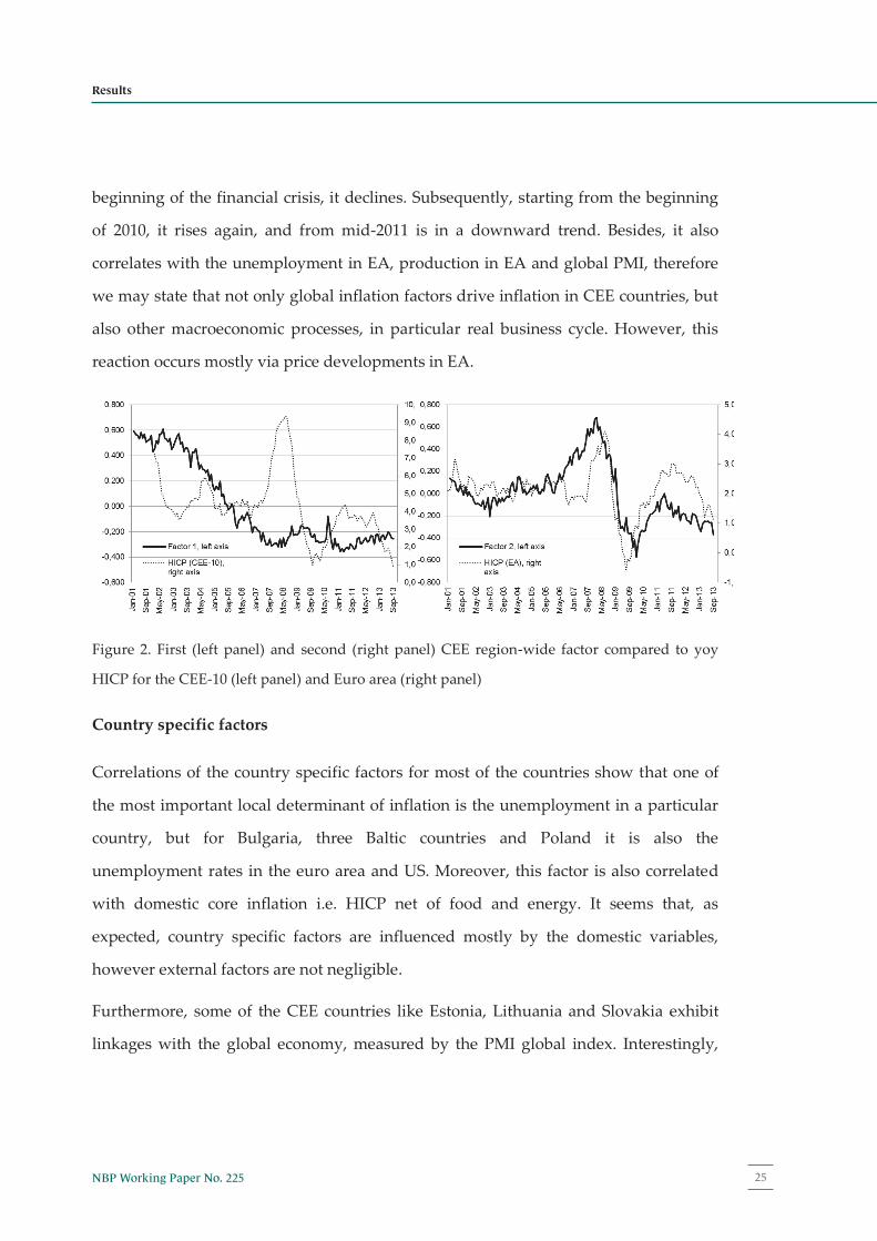
25NBP Working Paper No. 225
Results
23
The results indicate that the first factor may be associated with the disinflationary
processes that occurred in 2000s in some of CEE economies that led to a downturn in
inflation expectations. It can be seen, both, in lowering inflation in such CEE countries
like Bulgaria and Romania10 and in some of HICP components for several CEE
countries. This disinflationary process can be attributed to several factors. One factor is
an inflation targeting strategy which lowers inflation expectations. The other are
structural reforms conducted in the 90., which led to the change in the price setting
behavior of the firms. This process is also attributed to the globalization (Pehnelt 2007).
Its main face in CEE region is a relocation of production to the countries with relatively
lower labor costs, which is visible in the case of such consumption goods as garments,
footwear, equipment for recording, photography, recording media etc. Inflation
dynamics in those HICP components was either negative or in a downward trend. This
phenomenon is pointed out by Allard (2007) who evaluate the effect of the
globalization in Poland. According to this research globalization lowered prices in
Poland by 0.5 to 1 percentage point annually during 1995-2003 (more than in advanced
economies), which was possible by lowering the mark-ups. Moreover, Allard states
that this process will diminish after 2003 in line with the growing openness of the
countries. The shape of the first factor may support the course of globalization process
in CEE countries stated by Allard (2007).
The second factor can be recognized as a price reaction in the CEE countries to the
changes in the global economy, especially euro-area (EA) inflation, what we interpret
as an imported part of the country inflation in the region (see Figure 2). The second
factor fluctuates, similarly like HICP in the euro area, around zero level up to the end
of 2006, then it rises as the global commodity prices picked up and in 2009, with the
10 When eliminating Romania from the sample we would receive similar results – two comparable common factors, but in a reversed order of importance and with slightly lower part of overall variance explained.
24
beginning of the financial crisis, it declines. Subsequently, starting from the beginning
of 2010, it rises again, and from mid-2011 is in a downward trend. Besides, it also
correlates with the unemployment in EA, production in EA and global PMI, therefore
we may state that not only global inflation factors drive inflation in CEE countries, but
also other macroeconomic processes, in particular real business cycle. However, this
reaction occurs mostly via price developments in EA.
Figure 2. First (left panel) and second (right panel) CEE region-wide factor compared to yoy
HICP for the CEE-10 (left panel) and Euro area (right panel)
Country specific factors
Correlations of the country specific factors for most of the countries show that one of
the most important local determinant of inflation is the unemployment in a particular
country, but for Bulgaria, three Baltic countries and Poland it is also the
unemployment rates in the euro area and US. Moreover, this factor is also correlated
with domestic core inflation i.e. HICP net of food and energy. It seems that, as
expected, country specific factors are influenced mostly by the domestic variables,
however external factors are not negligible.
Furthermore, some of the CEE countries like Estonia, Lithuania and Slovakia exhibit
linkages with the global economy, measured by the PMI global index. Interestingly,
Narodowy Bank Polski26
25
Slovakia appears as a country strongly linked with the global commodity market,
especially with the price developments of the energy and industrial commodities. One
possible explanation is that it is a small country which experience quite high inflow of
foreign direct investments. As a matter of fact, Slovakia experienced one of the highest
inflow of the FDI (in relation to the GDP) among the CEE countries.
In general, countries with higher GDP per capita, higher productivity and economy’s
openness have on average higher volatility and lower persistence of the country factor
(which is especially visible in the case of the Baltic countries). This outcome can be
attributed to the fact that prices in those countries are more flexible (are changed more
often than in e.g. in the euro area, compare results for Estonia obtained by Dabušinskas
and Randveer, 2006). For small open economies quick adjustment to changing external
economy is important factor that helps to maintain the competitiveness of the domestic
companies. This higher elasticity of the domestic firms may steam from the lower
menu costs. In contrast, companies in the big countries, especially those with the big
domestic markets like Poland, can afford not to adjust so quickly to changing
environment due to the domestic demand.
Additionally, in our research we check whether exchange rate regime plays a role.
Countries with the fixed/pegged exchange rate (like Baltic countries or SI, BG) exhibit
higher volatility of country specific components, what suggests that floating exchange
rate and independent monetary policy may to some extent act as a shock absorber and
prevent against sharp movements in price indices in the period of global perturbations.
Sector specific factors
Developments of food prices in countries of the CEE region are driven by the changes
of the global commodity prices and also by domestic conditions. On one hand,
growing importance of the world commodity markets and the increasing openness of
the CEE economies causes stronger price reaction to the movements of the commodity
26
prices. On the other hand, recent research on the sensitivity of the HICP components to
the output gap in Poland provide evidence that more than half of food indices react to
the changes in the domestic output gap (see Hałka and Kotłowski, 2013). Similar
observation is valid for other non-durable goods, which include mainly the energy
products. The prices in this sector are strongly determined by the developments of
energy commodity prices (i.e. oil, gas and coal). The factors of second importance are
producer prices (PPI) and unemployment in the euro area. Quite strong correlation
with the PPI may be spurious, because PPI is strongly influenced by changes on the
commodity market. However, the correlation with the economic conditions of the euro
area proves that EA is an important partner for this sector.
The services group, according to the expectations, reveal the highest correlation with
the unemployment, especially with the unemployment in the analyzed countries,
though it is not a strong one. Services are rather a heterogeneous group which consists
of components influenced by strong competition (like communication or insurance
services) or administered to certain extent (like services related to dwellings). Such
components hardly react to changes in external or domestic economy (compare Hałka
and Kotłowski, 2013). Growing competitiveness and price deflation in some markets
are common for the economies in transition.
Surprisingly, there is hardly no influence of the changes in the global or domestic
economic activity on prices of durable and semi-durable goods. It is probably due to
the fact, that HICP components that encompass this groups are goods which prices are
influenced by the globalization process. Moreover, some of these goods are also under
strong impact of the technological developments (e.g. telephone equipment). Both
factors, globalization and technological development, entail lowering of prices no
matter what is the phase of the business cycle.
27NBP Working Paper No. 225
Results
25
Slovakia appears as a country strongly linked with the global commodity market,
especially with the price developments of the energy and industrial commodities. One
possible explanation is that it is a small country which experience quite high inflow of
foreign direct investments. As a matter of fact, Slovakia experienced one of the highest
inflow of the FDI (in relation to the GDP) among the CEE countries.
In general, countries with higher GDP per capita, higher productivity and economy’s
openness have on average higher volatility and lower persistence of the country factor
(which is especially visible in the case of the Baltic countries). This outcome can be
attributed to the fact that prices in those countries are more flexible (are changed more
often than in e.g. in the euro area, compare results for Estonia obtained by Dabušinskas
and Randveer, 2006). For small open economies quick adjustment to changing external
economy is important factor that helps to maintain the competitiveness of the domestic
companies. This higher elasticity of the domestic firms may steam from the lower
menu costs. In contrast, companies in the big countries, especially those with the big
domestic markets like Poland, can afford not to adjust so quickly to changing
environment due to the domestic demand.
Additionally, in our research we check whether exchange rate regime plays a role.
Countries with the fixed/pegged exchange rate (like Baltic countries or SI, BG) exhibit
higher volatility of country specific components, what suggests that floating exchange
rate and independent monetary policy may to some extent act as a shock absorber and
prevent against sharp movements in price indices in the period of global perturbations.
Sector specific factors
Developments of food prices in countries of the CEE region are driven by the changes
of the global commodity prices and also by domestic conditions. On one hand,
growing importance of the world commodity markets and the increasing openness of
the CEE economies causes stronger price reaction to the movements of the commodity
26
prices. On the other hand, recent research on the sensitivity of the HICP components to
the output gap in Poland provide evidence that more than half of food indices react to
the changes in the domestic output gap (see Hałka and Kotłowski, 2013). Similar
observation is valid for other non-durable goods, which include mainly the energy
products. The prices in this sector are strongly determined by the developments of
energy commodity prices (i.e. oil, gas and coal). The factors of second importance are
producer prices (PPI) and unemployment in the euro area. Quite strong correlation
with the PPI may be spurious, because PPI is strongly influenced by changes on the
commodity market. However, the correlation with the economic conditions of the euro
area proves that EA is an important partner for this sector.
The services group, according to the expectations, reveal the highest correlation with
the unemployment, especially with the unemployment in the analyzed countries,
though it is not a strong one. Services are rather a heterogeneous group which consists
of components influenced by strong competition (like communication or insurance
services) or administered to certain extent (like services related to dwellings). Such
components hardly react to changes in external or domestic economy (compare Hałka
and Kotłowski, 2013). Growing competitiveness and price deflation in some markets
are common for the economies in transition.
Surprisingly, there is hardly no influence of the changes in the global or domestic
economic activity on prices of durable and semi-durable goods. It is probably due to
the fact, that HICP components that encompass this groups are goods which prices are
influenced by the globalization process. Moreover, some of these goods are also under
strong impact of the technological developments (e.g. telephone equipment). Both
factors, globalization and technological development, entail lowering of prices no
matter what is the phase of the business cycle.
Narodowy Bank Polski28
Chapter 5
27
5. Conclusions
In this paper we apply a new method of multi-level factor model to decompose the
sources of time variation in a product-level inflation in each of 10 CEE countries. We
decompose the inflation rates into CEE region-wide, sector, country and country-sector
specific components.
We find that two regional factors explain about 17% of variance in monthly price
changes. The contribution of regional component varies considerably between different
countries and sectors. It is the most distinct determinant of inflation in Romania
(explaining 55% of price variability), and the least important for Estonia (10%), the
Czech Republic (8%) and Slovenia (6%). When the sectoral breakdown is concerned,
the CEE-wide component explains on average from 11% of variance in food and non-
durable sector to 24% in services being the most important price determinant in each of
them. Less important are country (6.5%), sector specific (3.1%) and country-sector
specific (9.6%) components. There are however single COICOP groups (liquid fuels,
garments), where the contribution of the two latter sectoral factors exceeds 50% of
variance in mom terms.
We also find the evidence that the regional component is very persistent (0.97 in terms
of AR1) and the country component is quite persistent too (0.68), which is generally in
line with similar studies for core EU countries. On the other hand, the average
standard deviation of aggregate and country-sector specific components (about 0.2 pp.
per month) is about twice as the volatility of country and sector-specific components.
In general, high volatility of macroeconomic components relative to sectoral ones is a
puzzling result in our study, which puts into the question the explanations provided
by the model of rational inattention.
Moreover, our research shows that product-level price changes in CEE countries are
more heterogeneous in terms of shock volatility across five sectors (e.g. services vs.
28
durable goods) than across ten countries. Such outcome may indicate the growing level
of economic integration in CEE region. We find that inflation in different sectors is
driven by very different forces; e.g. inflation in services is determined by
unemployment rate, whereas in durable goods is influenced by the external
inflationary processes such as globalization, level of inflation abroad. It means that
sectoral shocks influence prices dynamics more than country specific shocks and each
sector may react with a different scope and momentum to global disturbances.
The results also indicate that the first CEE-wide factor may be associated with the
disinflationary processes that occurred in CEE countries, whereas the second regional
factor reveals correlations with the global factors, especially commodity prices and
euro area aggregate HICP inflation. Additionally there is a higher volatility of the
country specific factors for countries with fixed exchange rate. Such outcome may
mean that floating exchange rate serves as a shock absorber and hampers the volatility
of the national prices.
As the sector specific factors are concerned prices of food and other non-durable goods
(mostly energy goods) strongly depend on the commodity markets. Prices of services
reveal the highest correlation with the unemployment in the analyzed countries,
though it is not a strong one. Surprisingly, there is hardly no influence of changes in
the global or domestic economic activity on prices of durable and semi-durable goods.
Probably, it is due to the fact, that HICP components that encompass these groups are
influenced by the globalization process, which leads to the price decreases regardless
the phase of the business cycle.
We leave two interesting questions for the further research. The first one is whether
there are some similarities between CEE and euro area countries in terms of product-
level inflation rates and the second is on the stability of this relationship over time.
29NBP Working Paper No. 225
Conclusions
27
5. Conclusions
In this paper we apply a new method of multi-level factor model to decompose the
sources of time variation in a product-level inflation in each of 10 CEE countries. We
decompose the inflation rates into CEE region-wide, sector, country and country-sector
specific components.
We find that two regional factors explain about 17% of variance in monthly price
changes. The contribution of regional component varies considerably between different
countries and sectors. It is the most distinct determinant of inflation in Romania
(explaining 55% of price variability), and the least important for Estonia (10%), the
Czech Republic (8%) and Slovenia (6%). When the sectoral breakdown is concerned,
the CEE-wide component explains on average from 11% of variance in food and non-
durable sector to 24% in services being the most important price determinant in each of
them. Less important are country (6.5%), sector specific (3.1%) and country-sector
specific (9.6%) components. There are however single COICOP groups (liquid fuels,
garments), where the contribution of the two latter sectoral factors exceeds 50% of
variance in mom terms.
We also find the evidence that the regional component is very persistent (0.97 in terms
of AR1) and the country component is quite persistent too (0.68), which is generally in
line with similar studies for core EU countries. On the other hand, the average
standard deviation of aggregate and country-sector specific components (about 0.2 pp.
per month) is about twice as the volatility of country and sector-specific components.
In general, high volatility of macroeconomic components relative to sectoral ones is a
puzzling result in our study, which puts into the question the explanations provided
by the model of rational inattention.
Moreover, our research shows that product-level price changes in CEE countries are
more heterogeneous in terms of shock volatility across five sectors (e.g. services vs.
28
durable goods) than across ten countries. Such outcome may indicate the growing level
of economic integration in CEE region. We find that inflation in different sectors is
driven by very different forces; e.g. inflation in services is determined by
unemployment rate, whereas in durable goods is influenced by the external
inflationary processes such as globalization, level of inflation abroad. It means that
sectoral shocks influence prices dynamics more than country specific shocks and each
sector may react with a different scope and momentum to global disturbances.
The results also indicate that the first CEE-wide factor may be associated with the
disinflationary processes that occurred in CEE countries, whereas the second regional
factor reveals correlations with the global factors, especially commodity prices and
euro area aggregate HICP inflation. Additionally there is a higher volatility of the
country specific factors for countries with fixed exchange rate. Such outcome may
mean that floating exchange rate serves as a shock absorber and hampers the volatility
of the national prices.
As the sector specific factors are concerned prices of food and other non-durable goods
(mostly energy goods) strongly depend on the commodity markets. Prices of services
reveal the highest correlation with the unemployment in the analyzed countries,
though it is not a strong one. Surprisingly, there is hardly no influence of changes in
the global or domestic economic activity on prices of durable and semi-durable goods.
Probably, it is due to the fact, that HICP components that encompass these groups are
influenced by the globalization process, which leads to the price decreases regardless
the phase of the business cycle.
We leave two interesting questions for the further research. The first one is whether
there are some similarities between CEE and euro area countries in terms of product-
level inflation rates and the second is on the stability of this relationship over time.
Narodowy Bank Polski30
References
29
References
Alexová, M., 2012. Inflation drivers in new EU members, Working paper 6/2012 NBS.
Allard, C., 2007. Inflation in Poland: How Much Can Globalization Explain?, IMF WP/07/41.
Altissimo, F., Benigno, P. and Palenzuela, D. R., 2011. Inflation Differentials in a Currency Area: Some Facts and Explanations, Open Economies Review, 22(2), 189-233.
Bai, J. and Ng, S., 2002. Determining the Number of Factors in Approximate Factor Models, 70(1), pp 191-221.
Bai, J. and Ng, S., 2013. Principal components estimation and identification of static factors, Journal of Econometrics 176 (2013), 18–29.
Ball, L. M., 2006. Has Globalization Changed Inflation? NBER Working Paper no. 12687.
Beck, G.W., Hubrich, K. and Marcellino, M., 2006. Regional Inflation Dynamics Within And Across Euro Area Countries And A Comparison With The US, Computing in Economics and Finance 2006 338, Society for Computational Economics.
Beck, G.W., Hubrich, K. and Marcellino, M., 2011. On The Importance Of Sectoral And Regional Shocks For Price-Setting, CEPR Discussion Papers 8357.
Bils, M. and Klenow, P. J., 2004. Some Evidence on the Importance of Sticky Prices, Journal of Political Economy, University of Chicago Press, 112(5), 947-985.
Bogoev, J., Petrevski and G., Sergi, B. S., 2012. Investigating the Link Between Central Bank Independence and Inflation in Central and Eastern Europe, Eastern European Economics, vol. 50, no. 4, pp. 78–96.
Boivin, J., Giannoni, M. P. and Mihov, I., 2009. Sticky Prices and Monetary Policy: Evidence from Disaggregated US Data, American Economic Review, 99(1), 350–384.
Borio, C. E. and Filardo, A. 2007. Globalisation and inflation: New cross-country evidence on the global determinants of domestic inflation, BIS Working Papers 227.
Breitung, J., Eickmeier, S., 2014. Analyzing business and financial cycles using multi-level factor models, Deutsche Bundesbank Discussion Paper 11/2014.
Choueiri, N., Ohnsorge, F. and van Elkan, R., 2008. Inflation Differentials in the EU: A Common (Factors) Approach with Implications for EU8 Euro Adoption Prospects, IMF WP/08/21.
Ciccarelli M. and Mojon B., 2010. Global Inflation, The Review of Economics and Statistics, MIT Press, 92(3), 524-535 (prev. EBC Working Paper 2005 no 537) .
30
Dabušinskas A. and M. Randveer, 2006. Comparison of pricing behaviour of firms in the euro area and Estonia, Bank of Estonia Working Papers 2006-08, Bank of Estonia, revised 10 Dec 2006.
Del Negro, M. and Otrok, C., 2008. Dynamic Factor Models with Time-Varying Parameters: Measuring Changes in International Business Cycles, Federal Reserve Bank of New York Staff Reports no. 326.
Eickmeier, S. and Kühnlenz M., 2013. China‘s role in global inflation dynamics, Discussion Paper Deutsche Bundesbank No 07/2013.
Forni, M., Hallin, M., Lippi, M. and Reichlin, L., 2000. The Generalized Dynamic-Factor Model: Identification And Estimation, The Review of Economics and Statistics, MIT Press, vol. 82(4), pages 540-554.
Hakkio, C. S., 2009. Global Inflation Dynamics, Federal Reserve Bank of Kansas City, Research Working Papers 09-01.
Hałka, A. and Kotłowski, J., 2013. Does domestic output gap matter for inflation in a small open economy?, Eastern European Economics, 52(3), 2014.
Kaufmann, D. and Lein, S.M., 2013. Sticky prices or rational inattention – What can we learn from sectoral price data? European Economic Review, 64, 384-394.
Kose, M. A., Otrok, Ch. and Whiteman, Ch.H., 2003. International Business Cycles: World, Region, and Country-Specific Factors, American Economic Review, 93(4), 1216-1239.
Krusper, B., 2012. The role of external and country specific factors in Hungarian inflation developments, MNB Working Papers 5 2012.
Maćkowiak, B., 2006. How Much of the Macroeconomic Variation in Eastern Europe is Attributable to External Shocks?, Comparative Economic Studies, Palgrave Macmillan, vol. 48(3), 523-544.
Maćkowiak, B., Moench, E. and Wiederholt, M., 2009. Sectoral Price Data and Models of Price Setting, Journal of Monetary Economics, 56, 78–99..
Maćkowiak, B. and Wiederholt, M., 2009. Optimal Sticky Prices under Rational Inattention, American Economic Review 2009, 99(3), 769–803.
Moench, E., Ng S. and Potter S., 2013. Dynamic hierarchical factor models, The Review of Economics and Statistics, 95(5), 1811-1817.
Monacelli, T. and Sala L., 2009. The International Dimension of Inflation: Evidence from Disaggregated Consumer Price Data, Journal of Money, Credit and Banking, Supplement to Vol. 41, No. 1.
Pehnelt, G., 2007. Globalisation and Inflation in OECD Countries, ECIPE Working Paper No. 04/2007.
31NBP Working Paper No. 225
References
29
References
Alexová, M., 2012. Inflation drivers in new EU members, Working paper 6/2012 NBS.
Allard, C., 2007. Inflation in Poland: How Much Can Globalization Explain?, IMF WP/07/41.
Altissimo, F., Benigno, P. and Palenzuela, D. R., 2011. Inflation Differentials in a Currency Area: Some Facts and Explanations, Open Economies Review, 22(2), 189-233.
Bai, J. and Ng, S., 2002. Determining the Number of Factors in Approximate Factor Models, 70(1), pp 191-221.
Bai, J. and Ng, S., 2013. Principal components estimation and identification of static factors, Journal of Econometrics 176 (2013), 18–29.
Ball, L. M., 2006. Has Globalization Changed Inflation? NBER Working Paper no. 12687.
Beck, G.W., Hubrich, K. and Marcellino, M., 2006. Regional Inflation Dynamics Within And Across Euro Area Countries And A Comparison With The US, Computing in Economics and Finance 2006 338, Society for Computational Economics.
Beck, G.W., Hubrich, K. and Marcellino, M., 2011. On The Importance Of Sectoral And Regional Shocks For Price-Setting, CEPR Discussion Papers 8357.
Bils, M. and Klenow, P. J., 2004. Some Evidence on the Importance of Sticky Prices, Journal of Political Economy, University of Chicago Press, 112(5), 947-985.
Bogoev, J., Petrevski and G., Sergi, B. S., 2012. Investigating the Link Between Central Bank Independence and Inflation in Central and Eastern Europe, Eastern European Economics, vol. 50, no. 4, pp. 78–96.
Boivin, J., Giannoni, M. P. and Mihov, I., 2009. Sticky Prices and Monetary Policy: Evidence from Disaggregated US Data, American Economic Review, 99(1), 350–384.
Borio, C. E. and Filardo, A. 2007. Globalisation and inflation: New cross-country evidence on the global determinants of domestic inflation, BIS Working Papers 227.
Breitung, J., Eickmeier, S., 2014. Analyzing business and financial cycles using multi-level factor models, Deutsche Bundesbank Discussion Paper 11/2014.
Choueiri, N., Ohnsorge, F. and van Elkan, R., 2008. Inflation Differentials in the EU: A Common (Factors) Approach with Implications for EU8 Euro Adoption Prospects, IMF WP/08/21.
Ciccarelli M. and Mojon B., 2010. Global Inflation, The Review of Economics and Statistics, MIT Press, 92(3), 524-535 (prev. EBC Working Paper 2005 no 537) .
30
Dabušinskas A. and M. Randveer, 2006. Comparison of pricing behaviour of firms in the euro area and Estonia, Bank of Estonia Working Papers 2006-08, Bank of Estonia, revised 10 Dec 2006.
Del Negro, M. and Otrok, C., 2008. Dynamic Factor Models with Time-Varying Parameters: Measuring Changes in International Business Cycles, Federal Reserve Bank of New York Staff Reports no. 326.
Eickmeier, S. and Kühnlenz M., 2013. China‘s role in global inflation dynamics, Discussion Paper Deutsche Bundesbank No 07/2013.
Forni, M., Hallin, M., Lippi, M. and Reichlin, L., 2000. The Generalized Dynamic-Factor Model: Identification And Estimation, The Review of Economics and Statistics, MIT Press, vol. 82(4), pages 540-554.
Hakkio, C. S., 2009. Global Inflation Dynamics, Federal Reserve Bank of Kansas City, Research Working Papers 09-01.
Hałka, A. and Kotłowski, J., 2013. Does domestic output gap matter for inflation in a small open economy?, Eastern European Economics, 52(3), 2014.
Kaufmann, D. and Lein, S.M., 2013. Sticky prices or rational inattention – What can we learn from sectoral price data? European Economic Review, 64, 384-394.
Kose, M. A., Otrok, Ch. and Whiteman, Ch.H., 2003. International Business Cycles: World, Region, and Country-Specific Factors, American Economic Review, 93(4), 1216-1239.
Krusper, B., 2012. The role of external and country specific factors in Hungarian inflation developments, MNB Working Papers 5 2012.
Maćkowiak, B., 2006. How Much of the Macroeconomic Variation in Eastern Europe is Attributable to External Shocks?, Comparative Economic Studies, Palgrave Macmillan, vol. 48(3), 523-544.
Maćkowiak, B., Moench, E. and Wiederholt, M., 2009. Sectoral Price Data and Models of Price Setting, Journal of Monetary Economics, 56, 78–99..
Maćkowiak, B. and Wiederholt, M., 2009. Optimal Sticky Prices under Rational Inattention, American Economic Review 2009, 99(3), 769–803.
Moench, E., Ng S. and Potter S., 2013. Dynamic hierarchical factor models, The Review of Economics and Statistics, 95(5), 1811-1817.
Monacelli, T. and Sala L., 2009. The International Dimension of Inflation: Evidence from Disaggregated Consumer Price Data, Journal of Money, Credit and Banking, Supplement to Vol. 41, No. 1.
Pehnelt, G., 2007. Globalisation and Inflation in OECD Countries, ECIPE Working Paper No. 04/2007.
Narodowy Bank Polski32
31
Staehr, K., 2010. Income Convergence and Inflation in Central and Eastern Europe Does the Sun Always Rise in the East?, Eastern European Economics, 48 (5), 38–62.
Stavrev, E., 2009. Forces Driving Inflation in the New EU10 Members, IMF WP/09/51.
Stock, J. and Watson, M., 2002. Macroeconomic Forecasting Using Diffusion Indexes, Journal of Business and Economic Statistics 20, 147-162.
32
Appendix 1 Decomposition results of the base case with two aggregate
factors
Table 4 Descriptive statistics of all-item HICP country indices (log monthly changes, SA)
BG CZ EE HU LT LV PL RO SI SK Descriptive statistics (inflation in terms of logarithmic mom changes)
Mean 0.388 0.178 0.330 0.378 0.252 0.402 0.217 0.718 0.290 0.308 Median 0.308 0.153 0.320 0.353 0.199 0.414 0.204 0.557 0.291 0.263 St. dev. 0.556 0.328 0.404 0.501 0.432 0.381 0.252 0.633 0.372 0.401 Skewness 0.637 1.831 0.533 0.506 1.099 -0.031 0.368 1.240 -0.074 1.877 Kurtosis 4.7 12.8 5.8 3.6 5.8 6.1 3.3 4.2 2.9 14.0 AR1 0.341 0.227 0.411 0.595 0.347 0.233 0.401 0.652 0.211 0.280
Source: Own calculations.
Table 5 Volatility, persistence and variance explained by estimated factors, cross-country
breakdown (log monthly changes)
BG CZ EE HU LT LV PL RO SI SK Volatility (St. dev.)
Aggregate 0.221 0.106 0.199 0.157 0.232 0.291 0.092 0.277 0.152 0.148 Country 0.112 0.082 0.154 0.134 0.131 0.145 0.086 0.081 0.161 0.104 Sector 0.162 0.085 0.169 0.090 0.126 0.168 0.071 0.067 0.178 0.101 Country-sector 0.201 0.126 0.217 0.135 0.166 0.228 0.095 0.127 0.256 0.154 Idiosyncratic 0.620 0.436 0.801 0.482 0.648 0.793 0.345 0.367 0.845 0.479 COICOP 0.232 0.189 0.281 0.193 0.253 0.317 0.152 0.133 0.252 0.212
Persistence (AR1) Aggregate 0.973 0.974 0.973 0.975 0.974 0.971 0.976 0.978 0.975 0.975 Country 0.698 0.635 0.621 0.660 0.690 0.592 0.883 0.849 -0.135 0.658 Sector 0.381 0.382 0.381 0.382 0.380 0.380 0.386 0.378 0.374 0.377 Country-sector 0.297 0.260 0.202 0.080 0.092 0.049 0.378 0.523 -0.021 0.367 Idiosyncratic 0.119 0.037 0.024 0.070 0.049 -0.010 0.139 0.234 -0.053 0.095 COICOP 0.153 0.146 0.149 0.148 0.147 0.148 0.151 0.148 0.144 0.148
Variance explained Aggregate 0.183 0.085 0.098 0.161 0.178 0.161 0.134 0.548 0.056 0.125 Country 0.046 0.047 0.040 0.090 0.041 0.044 0.196 0.036 0.037 0.062 Sector 0.037 0.028 0.037 0.027 0.032 0.039 0.029 0.015 0.034 0.032 Country-sector 0.078 0.087 0.095 0.082 0.082 0.079 0.089 0.060 0.100 0.092 Idiosyncratic 0.656 0.753 0.731 0.639 0.665 0.678 0.551 0.340 0.773 0.687 COICOP 0.107 0.134 0.112 0.110 0.110 0.118 0.117 0.056 0.080 0.147
Squared loadings at two aggregate factors Aggregate 1 0.059 0.051 0.023 0.112 0.065 0.020 0.074 0.484 0.031 0.081 Aggregate 2 0.180 0.053 0.104 0.063 0.174 0.208 0.084 0.043 0.032 0.058
Source: Own calculations.
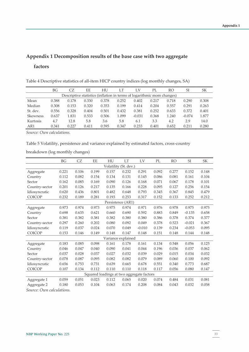
33NBP Working Paper No. 225
Appendix 1
31
Staehr, K., 2010. Income Convergence and Inflation in Central and Eastern Europe Does the Sun Always Rise in the East?, Eastern European Economics, 48 (5), 38–62.
Stavrev, E., 2009. Forces Driving Inflation in the New EU10 Members, IMF WP/09/51.
Stock, J. and Watson, M., 2002. Macroeconomic Forecasting Using Diffusion Indexes, Journal of Business and Economic Statistics 20, 147-162.
32
Appendix 1 Decomposition results of the base case with two aggregate
factors
Table 4 Descriptive statistics of all-item HICP country indices (log monthly changes, SA)
BG CZ EE HU LT LV PL RO SI SK Descriptive statistics (inflation in terms of logarithmic mom changes)
Mean 0.388 0.178 0.330 0.378 0.252 0.402 0.217 0.718 0.290 0.308 Median 0.308 0.153 0.320 0.353 0.199 0.414 0.204 0.557 0.291 0.263 St. dev. 0.556 0.328 0.404 0.501 0.432 0.381 0.252 0.633 0.372 0.401 Skewness 0.637 1.831 0.533 0.506 1.099 -0.031 0.368 1.240 -0.074 1.877 Kurtosis 4.7 12.8 5.8 3.6 5.8 6.1 3.3 4.2 2.9 14.0 AR1 0.341 0.227 0.411 0.595 0.347 0.233 0.401 0.652 0.211 0.280
Source: Own calculations.
Table 5 Volatility, persistence and variance explained by estimated factors, cross-country
breakdown (log monthly changes)
BG CZ EE HU LT LV PL RO SI SK Volatility (St. dev.)
Aggregate 0.221 0.106 0.199 0.157 0.232 0.291 0.092 0.277 0.152 0.148 Country 0.112 0.082 0.154 0.134 0.131 0.145 0.086 0.081 0.161 0.104 Sector 0.162 0.085 0.169 0.090 0.126 0.168 0.071 0.067 0.178 0.101 Country-sector 0.201 0.126 0.217 0.135 0.166 0.228 0.095 0.127 0.256 0.154 Idiosyncratic 0.620 0.436 0.801 0.482 0.648 0.793 0.345 0.367 0.845 0.479 COICOP 0.232 0.189 0.281 0.193 0.253 0.317 0.152 0.133 0.252 0.212
Persistence (AR1) Aggregate 0.973 0.974 0.973 0.975 0.974 0.971 0.976 0.978 0.975 0.975 Country 0.698 0.635 0.621 0.660 0.690 0.592 0.883 0.849 -0.135 0.658 Sector 0.381 0.382 0.381 0.382 0.380 0.380 0.386 0.378 0.374 0.377 Country-sector 0.297 0.260 0.202 0.080 0.092 0.049 0.378 0.523 -0.021 0.367 Idiosyncratic 0.119 0.037 0.024 0.070 0.049 -0.010 0.139 0.234 -0.053 0.095 COICOP 0.153 0.146 0.149 0.148 0.147 0.148 0.151 0.148 0.144 0.148
Variance explained Aggregate 0.183 0.085 0.098 0.161 0.178 0.161 0.134 0.548 0.056 0.125 Country 0.046 0.047 0.040 0.090 0.041 0.044 0.196 0.036 0.037 0.062 Sector 0.037 0.028 0.037 0.027 0.032 0.039 0.029 0.015 0.034 0.032 Country-sector 0.078 0.087 0.095 0.082 0.082 0.079 0.089 0.060 0.100 0.092 Idiosyncratic 0.656 0.753 0.731 0.639 0.665 0.678 0.551 0.340 0.773 0.687 COICOP 0.107 0.134 0.112 0.110 0.110 0.118 0.117 0.056 0.080 0.147
Squared loadings at two aggregate factors Aggregate 1 0.059 0.051 0.023 0.112 0.065 0.020 0.074 0.484 0.031 0.081 Aggregate 2 0.180 0.053 0.104 0.063 0.174 0.208 0.084 0.043 0.032 0.058
Source: Own calculations.
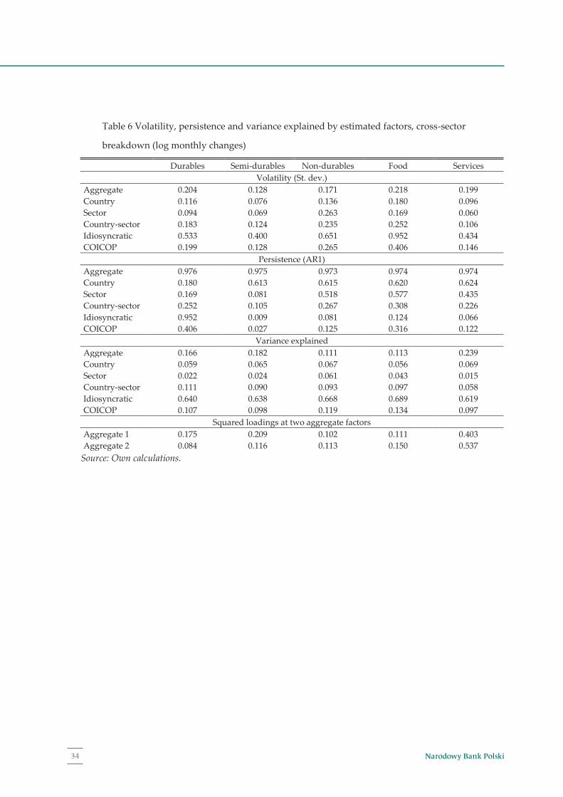
Narodowy Bank Polski34
33
Table 6 Volatility, persistence and variance explained by estimated factors, cross-sector
breakdown (log monthly changes)
Durables Semi-durables Non-durables Food Services Volatility (St. dev.)
Aggregate 0.204 0.128 0.171 0.218 0.199 Country 0.116 0.076 0.136 0.180 0.096 Sector 0.094 0.069 0.263 0.169 0.060 Country-sector 0.183 0.124 0.235 0.252 0.106 Idiosyncratic 0.533 0.400 0.651 0.952 0.434 COICOP 0.199 0.128 0.265 0.406 0.146
Persistence (AR1) Aggregate 0.976 0.975 0.973 0.974 0.974 Country 0.180 0.613 0.615 0.620 0.624 Sector 0.169 0.081 0.518 0.577 0.435 Country-sector 0.252 0.105 0.267 0.308 0.226 Idiosyncratic 0.952 0.009 0.081 0.124 0.066 COICOP 0.406 0.027 0.125 0.316 0.122
Variance explained Aggregate 0.166 0.182 0.111 0.113 0.239 Country 0.059 0.065 0.067 0.056 0.069 Sector 0.022 0.024 0.061 0.043 0.015 Country-sector 0.111 0.090 0.093 0.097 0.058 Idiosyncratic 0.640 0.638 0.668 0.689 0.619 COICOP 0.107 0.098 0.119 0.134 0.097
Squared loadings at two aggregate factors Aggregate 1 0.175 0.209 0.102 0.111 0.403 Aggregate 2 0.084 0.116 0.113 0.150 0.537
Source: Own calculations.
34
Appendix 2 Robustness analysis
Figure 3 Scree plots of correlation matrix in a balanced panel of product-level HICPs
Source: Own calculations
Table 7 Volatility, persistence and fraction of variance explained by components of factor model
decomposition with three aggregate factors (monthly log changes)
Aggregate Country Sector Country-sector
Idiosyncratic COICOP
Volatility (St. dev.) Mean 0.214 0.109 0.129 0.172 0.568 0.215
Median 0.177 0.068 0.043 0.094 0.392 0.123
Min 0.007 0.000 0.000 0.000 0.021 0.000
Max 1.083 1.305 3.390 1.800 4.514 3.474
St. dev. 0.150 0.139 0.293 0.224 0.601 0.331 Persistence (AR1)
Mean 0.960 0.423 0.470 0.190 0.056 0.139
Median 0.968 0.507 0.625 0.208 0.045 0.108
Min 0.907 -0.169 0.157 -0.282 -0.550 -0.302
Max 0.984 0.832 0.629 0.613 0.690 0.657
St. dev. 0.020 0.279 0.194 0.206 0.172 0.195 Variance explained
Mean 0.210 0.041 0.034 0.080 0.630 0.105
Median 0.128 0.020 0.009 0.043 0.661 0.081
Min 0.001 0.000 0.000 0.000 0.024 0.000
Max 0.916 0.310 0.634 0.588 0.989 0.529
St. dev. 0.216 0.052 0.076 0.095 0.221 0.103
Source: Own calculations.
1 2 3 4 5 6 7 8 9 10 11 12 13 14 150
0.02
0.04
0.06
0.08
0.1
0.12Eigenvalues of aggregate factors (mom log changes)
1 2 3 4 5 6 7 8 9 10 11 12 13 14 150
0.05
0.1
0.15
0.2Eigenvalues of aggregate factors (yoy log changes)
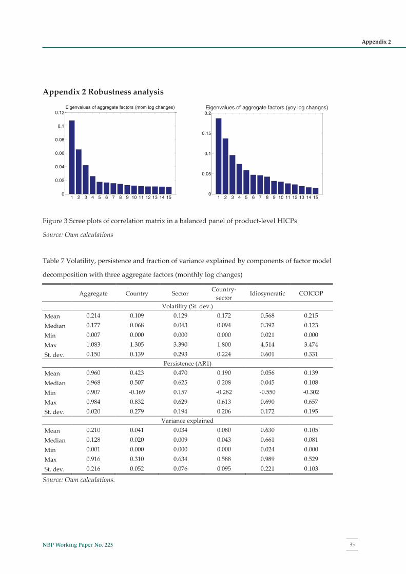
35NBP Working Paper No. 225
Appendix 2
33
Table 6 Volatility, persistence and variance explained by estimated factors, cross-sector
breakdown (log monthly changes)
Durables Semi-durables Non-durables Food Services Volatility (St. dev.)
Aggregate 0.204 0.128 0.171 0.218 0.199 Country 0.116 0.076 0.136 0.180 0.096 Sector 0.094 0.069 0.263 0.169 0.060 Country-sector 0.183 0.124 0.235 0.252 0.106 Idiosyncratic 0.533 0.400 0.651 0.952 0.434 COICOP 0.199 0.128 0.265 0.406 0.146
Persistence (AR1) Aggregate 0.976 0.975 0.973 0.974 0.974 Country 0.180 0.613 0.615 0.620 0.624 Sector 0.169 0.081 0.518 0.577 0.435 Country-sector 0.252 0.105 0.267 0.308 0.226 Idiosyncratic 0.952 0.009 0.081 0.124 0.066 COICOP 0.406 0.027 0.125 0.316 0.122
Variance explained Aggregate 0.166 0.182 0.111 0.113 0.239 Country 0.059 0.065 0.067 0.056 0.069 Sector 0.022 0.024 0.061 0.043 0.015 Country-sector 0.111 0.090 0.093 0.097 0.058 Idiosyncratic 0.640 0.638 0.668 0.689 0.619 COICOP 0.107 0.098 0.119 0.134 0.097
Squared loadings at two aggregate factors Aggregate 1 0.175 0.209 0.102 0.111 0.403 Aggregate 2 0.084 0.116 0.113 0.150 0.537
Source: Own calculations.
34
Appendix 2 Robustness analysis
Figure 3 Scree plots of correlation matrix in a balanced panel of product-level HICPs
Source: Own calculations
Table 7 Volatility, persistence and fraction of variance explained by components of factor model
decomposition with three aggregate factors (monthly log changes)
Aggregate Country Sector Country-sector
Idiosyncratic COICOP
Volatility (St. dev.) Mean 0.214 0.109 0.129 0.172 0.568 0.215
Median 0.177 0.068 0.043 0.094 0.392 0.123
Min 0.007 0.000 0.000 0.000 0.021 0.000
Max 1.083 1.305 3.390 1.800 4.514 3.474
St. dev. 0.150 0.139 0.293 0.224 0.601 0.331 Persistence (AR1)
Mean 0.960 0.423 0.470 0.190 0.056 0.139
Median 0.968 0.507 0.625 0.208 0.045 0.108
Min 0.907 -0.169 0.157 -0.282 -0.550 -0.302
Max 0.984 0.832 0.629 0.613 0.690 0.657
St. dev. 0.020 0.279 0.194 0.206 0.172 0.195 Variance explained
Mean 0.210 0.041 0.034 0.080 0.630 0.105
Median 0.128 0.020 0.009 0.043 0.661 0.081
Min 0.001 0.000 0.000 0.000 0.024 0.000
Max 0.916 0.310 0.634 0.588 0.989 0.529
St. dev. 0.216 0.052 0.076 0.095 0.221 0.103
Source: Own calculations.
1 2 3 4 5 6 7 8 9 10 11 12 13 14 150
0.02
0.04
0.06
0.08
0.1
0.12Eigenvalues of aggregate factors (mom log changes)
1 2 3 4 5 6 7 8 9 10 11 12 13 14 150
0.05
0.1
0.15
0.2Eigenvalues of aggregate factors (yoy log changes)
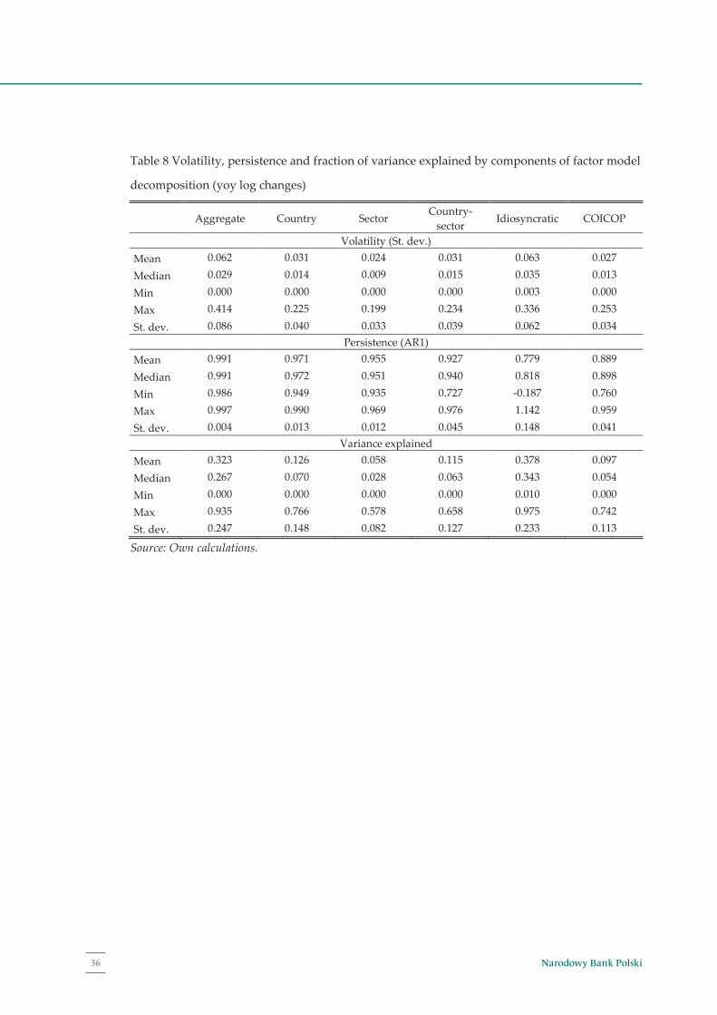
Narodowy Bank Polski36
35
Table 8 Volatility, persistence and fraction of variance explained by components of factor model
decomposition (yoy log changes)
Aggregate Country Sector Country-sector
Idiosyncratic COICOP
Volatility (St. dev.) Mean 0.062 0.031 0.024 0.031 0.063 0.027
Median 0.029 0.014 0.009 0.015 0.035 0.013
Min 0.000 0.000 0.000 0.000 0.003 0.000
Max 0.414 0.225 0.199 0.234 0.336 0.253
St. dev. 0.086 0.040 0.033 0.039 0.062 0.034 Persistence (AR1)
Mean 0.991 0.971 0.955 0.927 0.779 0.889
Median 0.991 0.972 0.951 0.940 0.818 0.898
Min 0.986 0.949 0.935 0.727 -0.187 0.760
Max 0.997 0.990 0.969 0.976 1.142 0.959
St. dev. 0.004 0.013 0.012 0.045 0.148 0.041 Variance explained
Mean 0.323 0.126 0.058 0.115 0.378 0.097
Median 0.267 0.070 0.028 0.063 0.343 0.054
Min 0.000 0.000 0.000 0.000 0.010 0.000
Max 0.935 0.766 0.578 0.658 0.975 0.742
St. dev. 0.247 0.148 0.082 0.127 0.233 0.113
Source: Own calculations.

www.nbp.pl