
type="text/javascript" >
72
Fundamental of Image Processing By Ashis Kr. Dhara 1
-
Upload
ganeshss007 -
Category
Documents
-
view
230 -
download
0
Transcript of type="text/javascript" >
Fundamental of Image Processing
By
Ashis Kr. Dhara
1
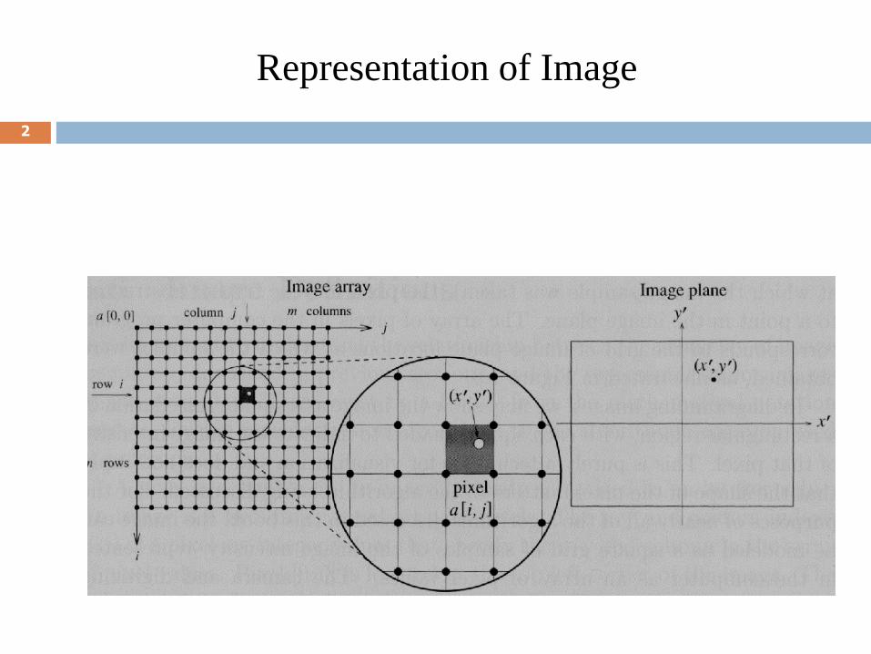
Representation of Image
2

Point Processing
3
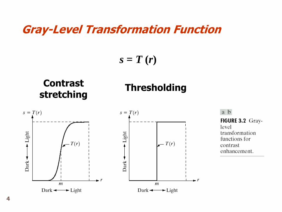
Gray-Level Transformation Function
s = T (r)
Contrast stretching
Thresholding
4
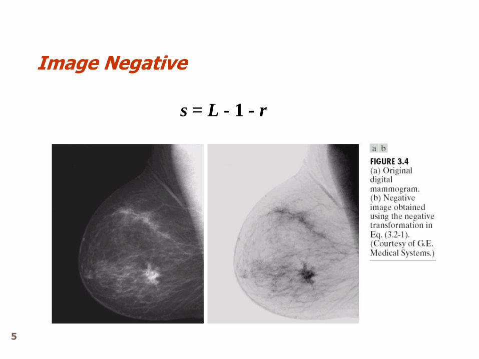
Image Negative
s = L - 1 - r
5
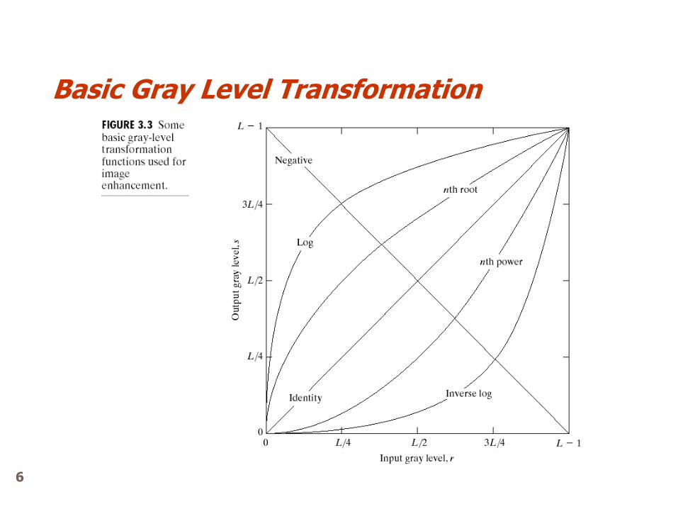
Basic Gray Level Transformation
6
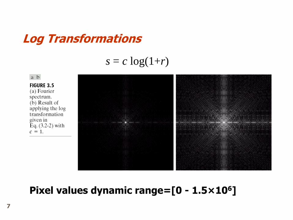
Log Transformations
s = c log(1+r)
Pixel values dynamic range=[0 - 1.5×10⁶]
7
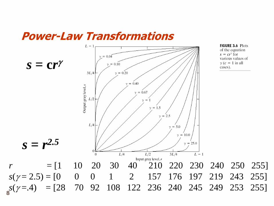
Power-Law Transformations
s = cr
s = r2.5
r = [1 10 20 30 40 210 220 230 240 250 255]
s( = 2.5) = [0 0 0 1 2 157 176 197 219 243 255]
s( =.4) = [28 70 92 108 122 236 240 245 249 253 255] 8
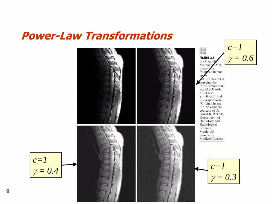
Power-Law Transformations
c=1
= 0.4 c=1
= 0.3
c=1
= 0.6
9
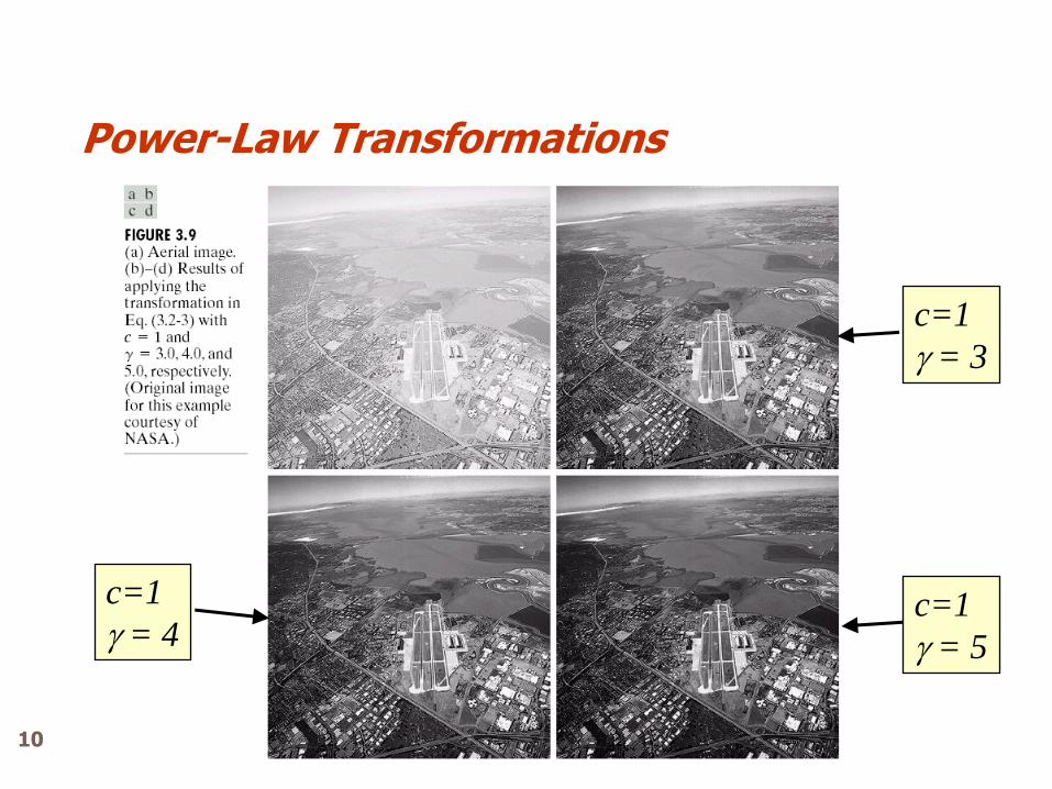
Power-Law Transformations
c=1
= 3
c=1
= 5
c=1
= 4
10
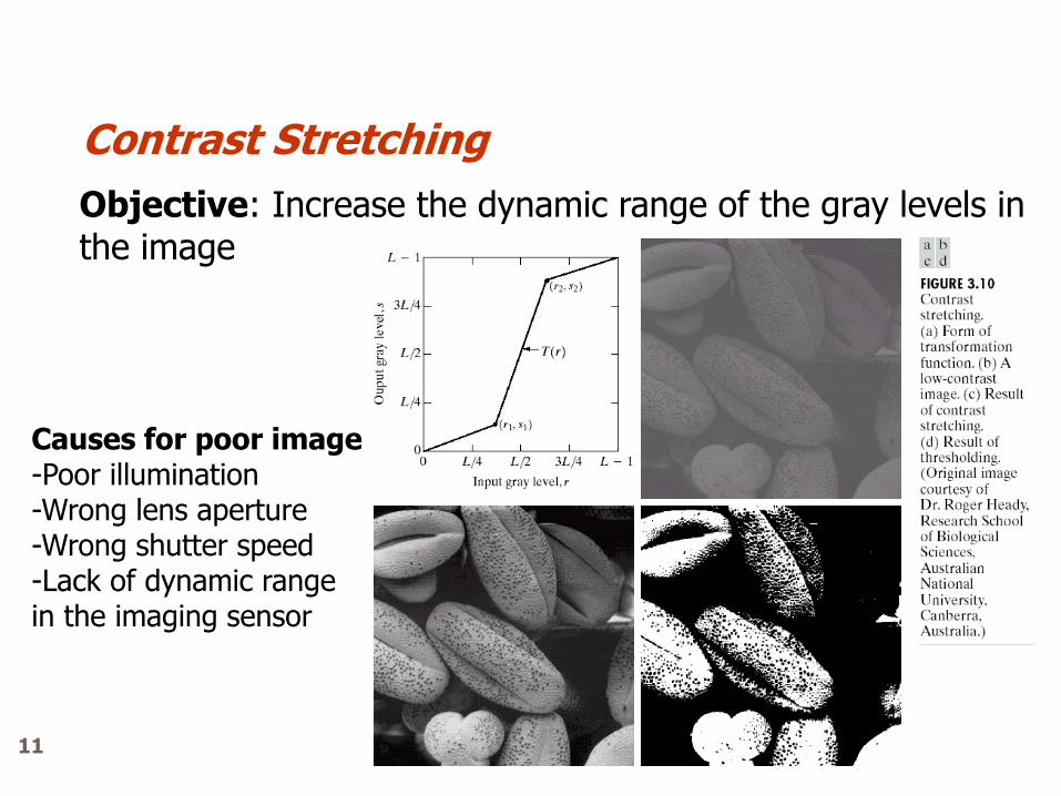
Contrast Stretching
Objective: Increase the dynamic range of the gray levels in the image
Causes for poor image -Poor illumination -Wrong lens aperture -Wrong shutter speed -Lack of dynamic range in the imaging sensor
11
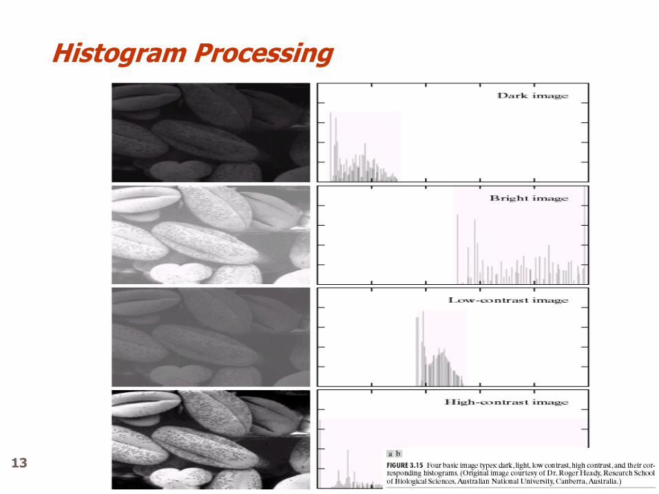
Histogram The histogram of a digital image with gray levels in the range [0, L-1] is a discrete function h(rk) = nk, where rk is the kth gray level and nk is the number of pixels in the image having gray level rk.
Normalized Histogram Dividing each value of the histogram by the total number of pixels in the image, denoted by n. p(rk) = nk /n. Normalized histogram provide useful image statistics.
Histogram Processing
12
Histogram Processing
13
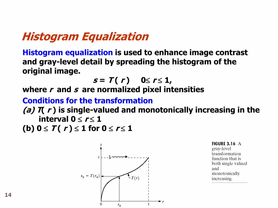
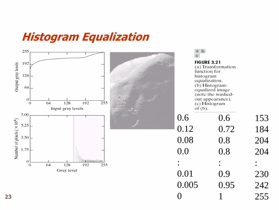
Histogram equalization is used to enhance image contrast and gray-level detail by spreading the histogram of the original image. s = T ( r ) 0 r 1, where r and s are normalized pixel intensities
Conditions for the transformation (a) T( r ) is single-valued and monotonically increasing in the interval 0 r 1 (b) 0 T ( r ) 1 for 0 r 1
1
Histogram Equalization
14
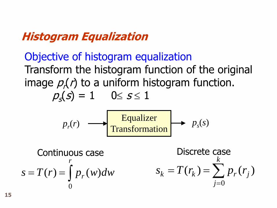
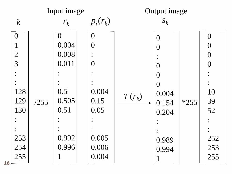
Objective of histogram equalization Transform the histogram function of the original image pr(r) to a uniform histogram function. ps(s) = 1 0 s 1
Equalizer
Transformation pr(r) ps(s)
r
r dwwprTs
0
)()(
k
j
jrkk rprTs0
)()(
Continuous case Discrete case
Histogram Equalization
15
0
1
2
3
:
:
128
129
130
:
:
253
254
255
0
0
:
0
:
:
0.004
0.15
0.05
:
:
0.005
0.006
0.004
pr(rk) k
T (rk)
0
0
:
0
0
0
0.004
0.154
0.204
:
:
0.989
0.994
1
sk
0
0
0
0
:
:
10
39
52
:
:
252
253
255
0
0.004
0.008
0.011
:
:
0.5
0.505
0.51
:
:
0.992
0.996
1
rk
/255 *255
Input image Output image
16
Histogram Equalization
17
Histogram Equalization
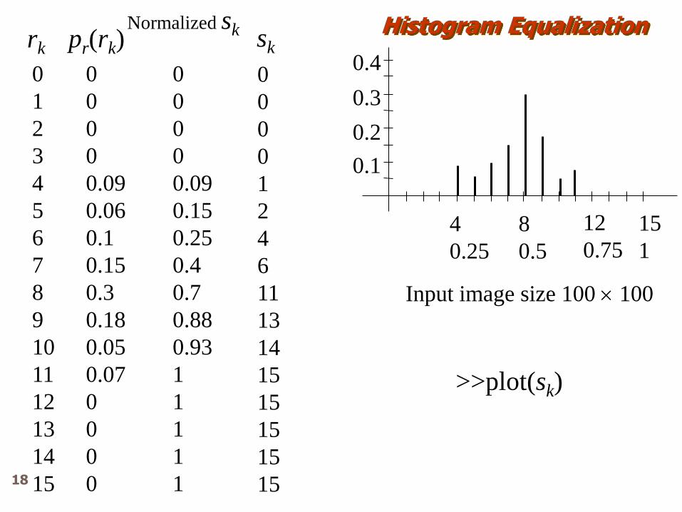
15
1
8
0.5
4
0.25
12
0.75
0.4
0.2
0.3
0.1
0
1
2
3
4
5
6
7
8
9
10
11
12
13
14
15
0
0
0
0
0.09
0.06
0.1
0.15
0.3
0.18
0.05
0.07
0
0
0
0
0
0
0
0
0.09
0.15
0.25
0.4
0.7
0.88
0.93
1
1
1
1
1
rk pr(rk) Normalized sk
0
0
0
0
1
2
4
6
11
13
14
15
15
15
15
15
sk
>>plot(sk)
Input image size 100 100
18
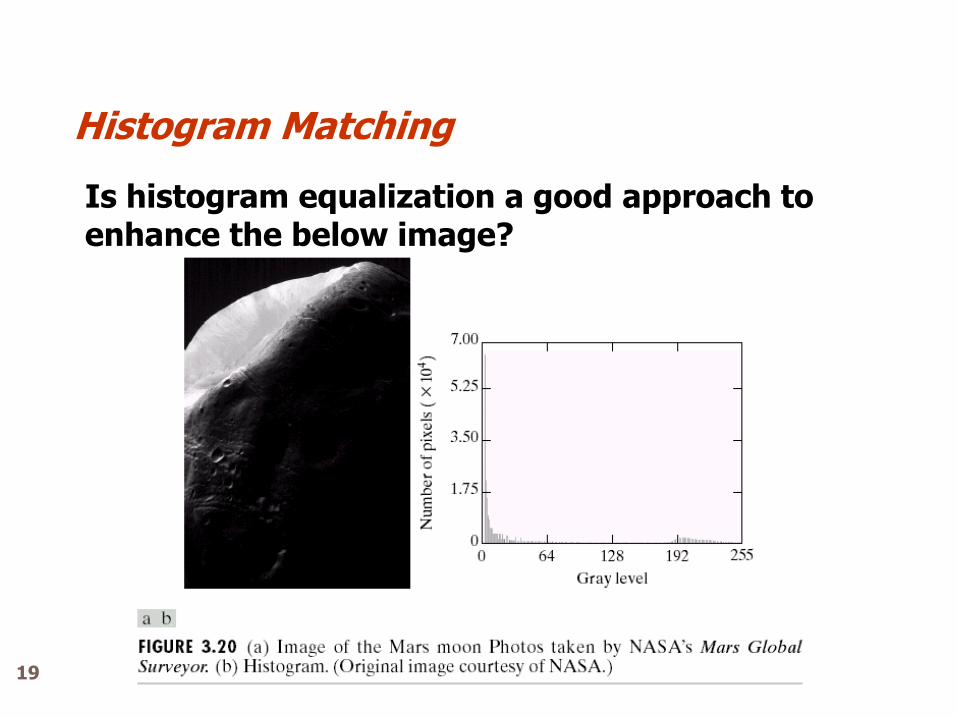
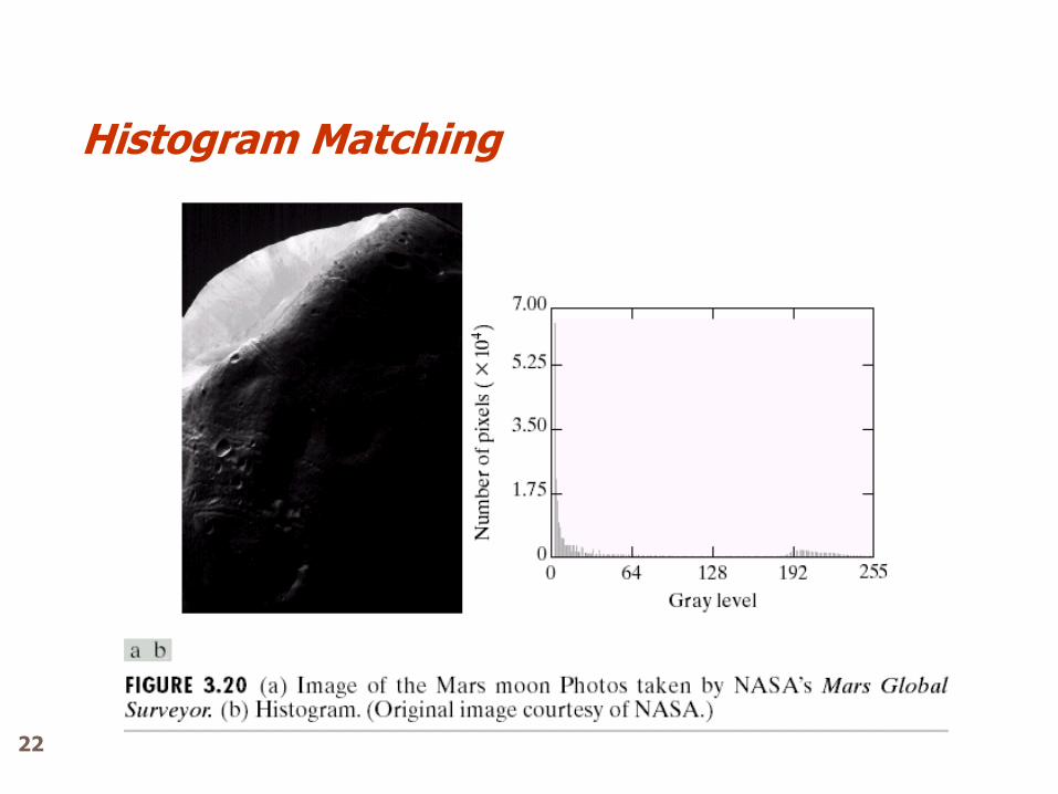
Is histogram equalization a good approach to enhance the below image?
Histogram Matching
19
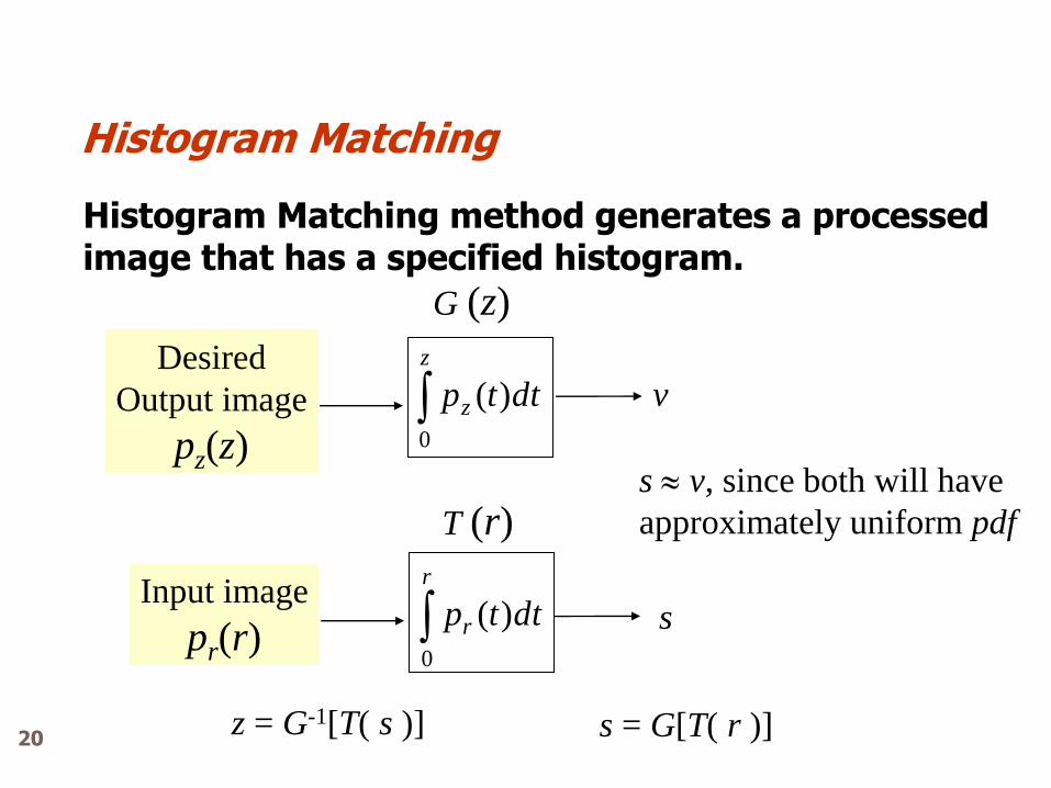
Histogram Matching method generates a processed image that has a specified histogram.
Input image
pr(r)
T (r)
r
r dttp
0
)( s
Desired
Output image
pz(z)
G (z)
z
z dttp
0
)( v
s v, since both will have
approximately uniform pdf
z = G-1[T( s )] s = G[T( r )]
Histogram Matching
20
Histogram Matching
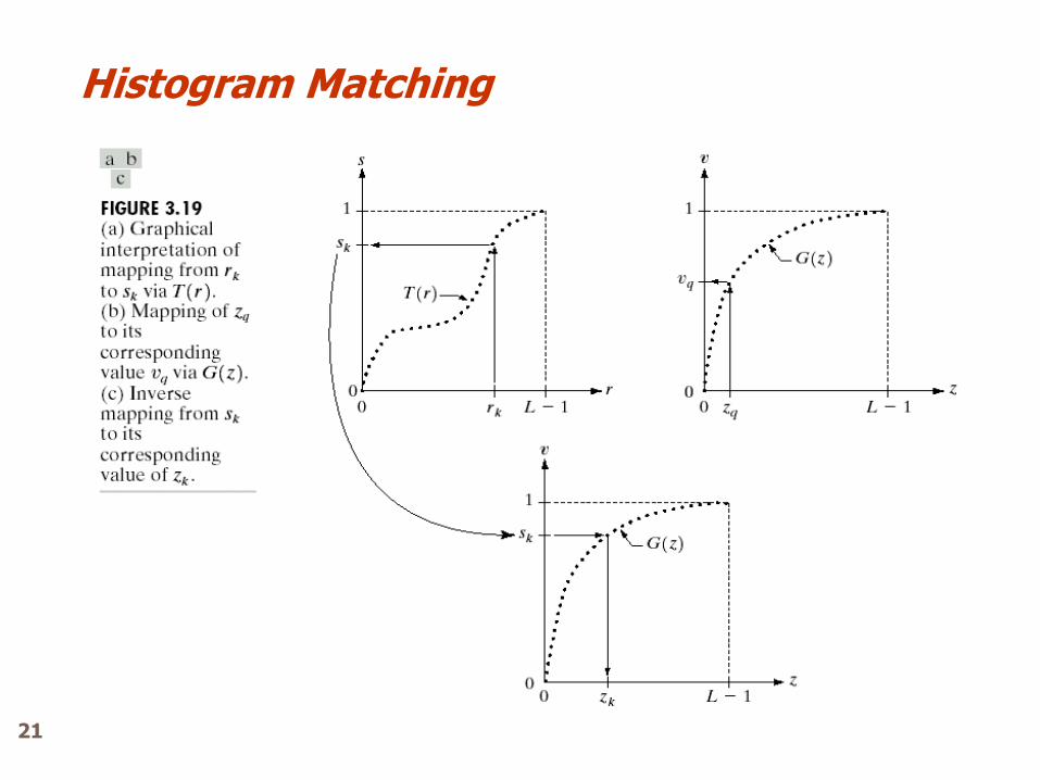
21
Histogram Matching
22
0.6
0.12
0.08
0.0
:
0.01
0.005
0
0.6
0.72
0.8
0.8
:
0.9
0.95
1
153
184
204
204
:
230
242
255
Histogram Equalization
23
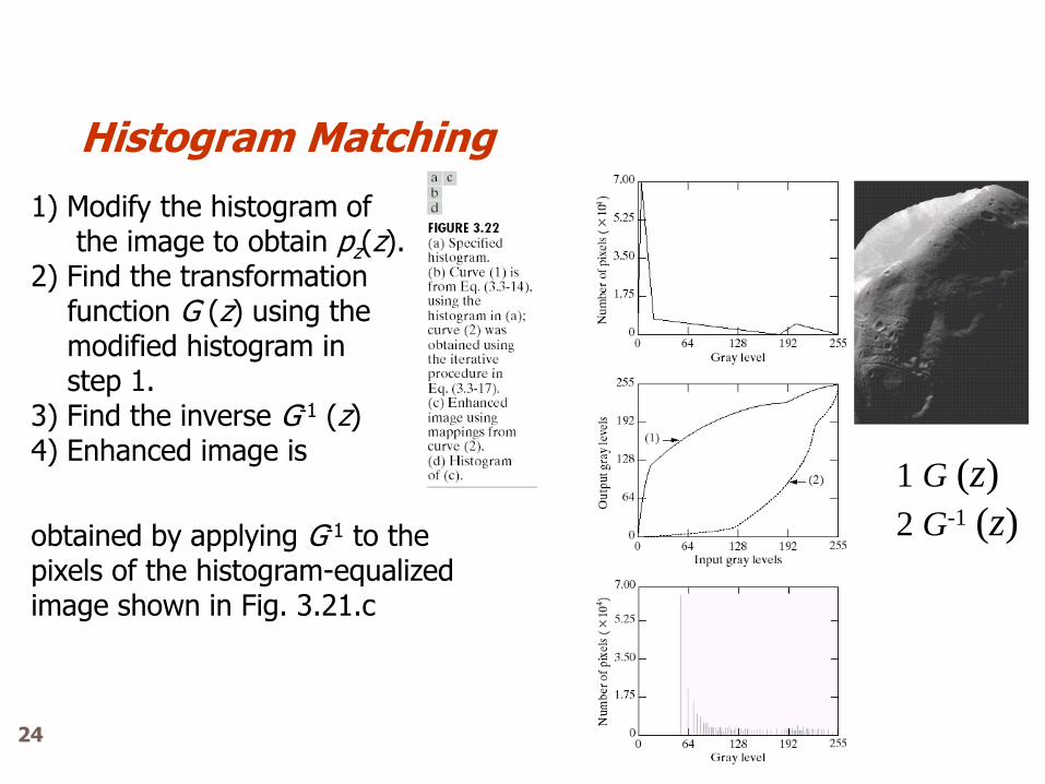
1) Modify the histogram of the image to obtain pz(z). 2) Find the transformation function G (z) using the modified histogram in step 1. 3) Find the inverse G-1 (z) 4) Enhanced image is
obtained by applying G-1 to the pixels of the histogram-equalized image shown in Fig. 3.21.c
1 G (z)
2 G-1 (z)
Histogram Matching
24
Arithmetic/logic operations involving images are performed on a pixel-by-pixel basis between two or more images. Arithmetic Operations Addition, Subtraction, Multiplication, and Division Logic Operations AND, OR, NOT
Enhancement Using Arithmetic/Logic Op.
25

AND
OR
Logic operations are performed on the binary representation of the pixel intensities
Enhancement Using AND and OR Logic Op.
26
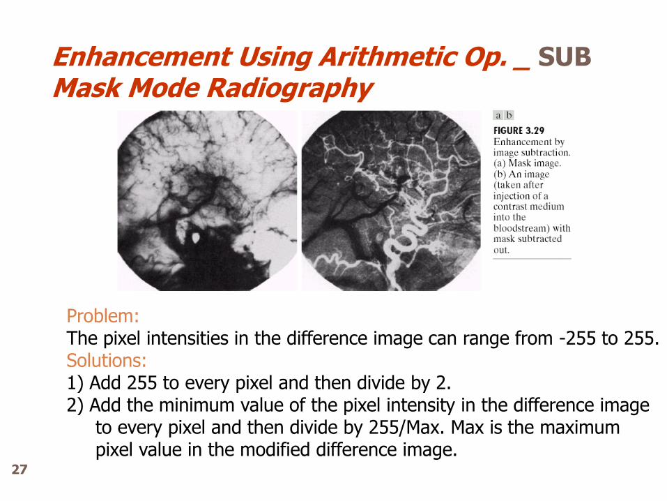
Problem: The pixel intensities in the difference image can range from -255 to 255. Solutions: 1) Add 255 to every pixel and then divide by 2. 2) Add the minimum value of the pixel intensity in the difference image to every pixel and then divide by 255/Max. Max is the maximum pixel value in the modified difference image.
Enhancement Using Arithmetic Op. _ SUB Mask Mode Radiography
27
Spatial Filtering
28
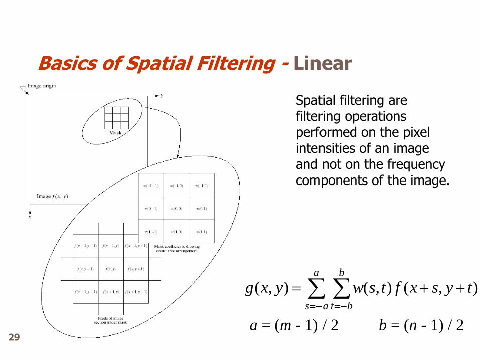
Spatial filtering are filtering operations performed on the pixel intensities of an image and not on the frequency components of the image.
a
as
b
bt
tysxftswyxg ),(),(),(
a = (m - 1) / 2 b = (n - 1) / 2
Basics of Spatial Filtering - Linear
29
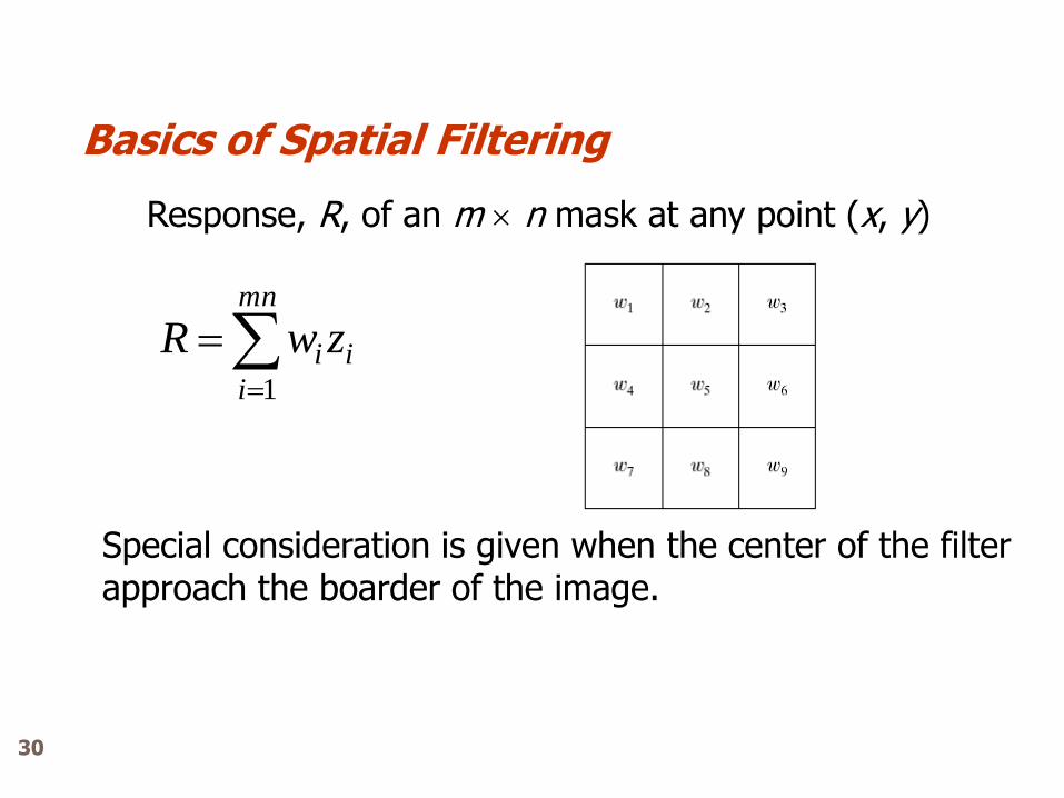
Response, R, of an m n mask at any point (x, y)
mn
i
iizwR1
Special consideration is given when the center of the filter approach the boarder of the image.
Basics of Spatial Filtering
30
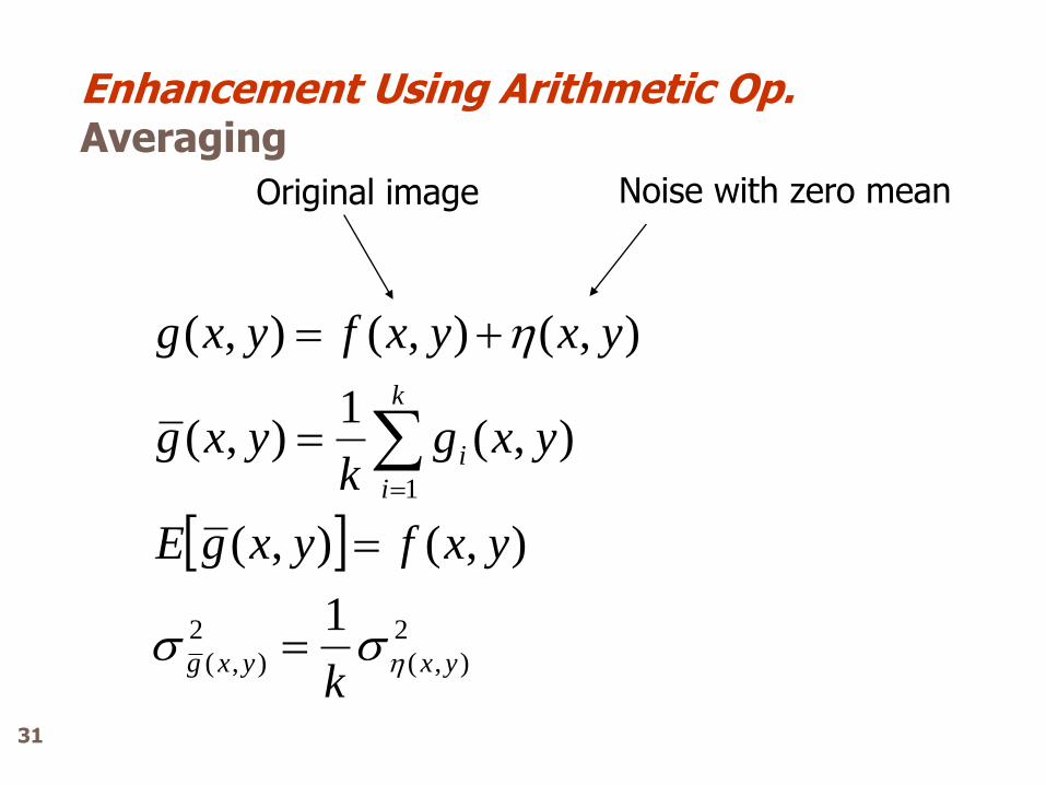
2
),(
2
),(
1
1
),(),(
),(1
),(
),(),(),(
yxyxg
k
i
i
k
yxfyxgE
yxgk
yxg
yxyxfyxg
Original image Noise with zero mean
Enhancement Using Arithmetic Op. Averaging
31
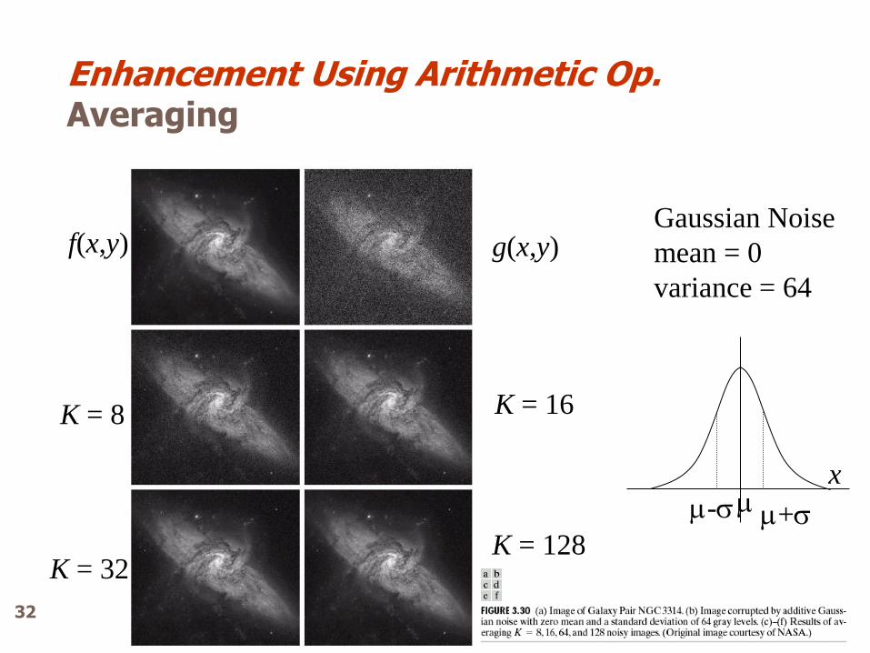
Gaussian Noise
mean = 0
variance = 64
K = 8
K = 32
K = 16
K = 128
f(x,y) g(x,y)
+ -
x
Enhancement Using Arithmetic Op. Averaging
32
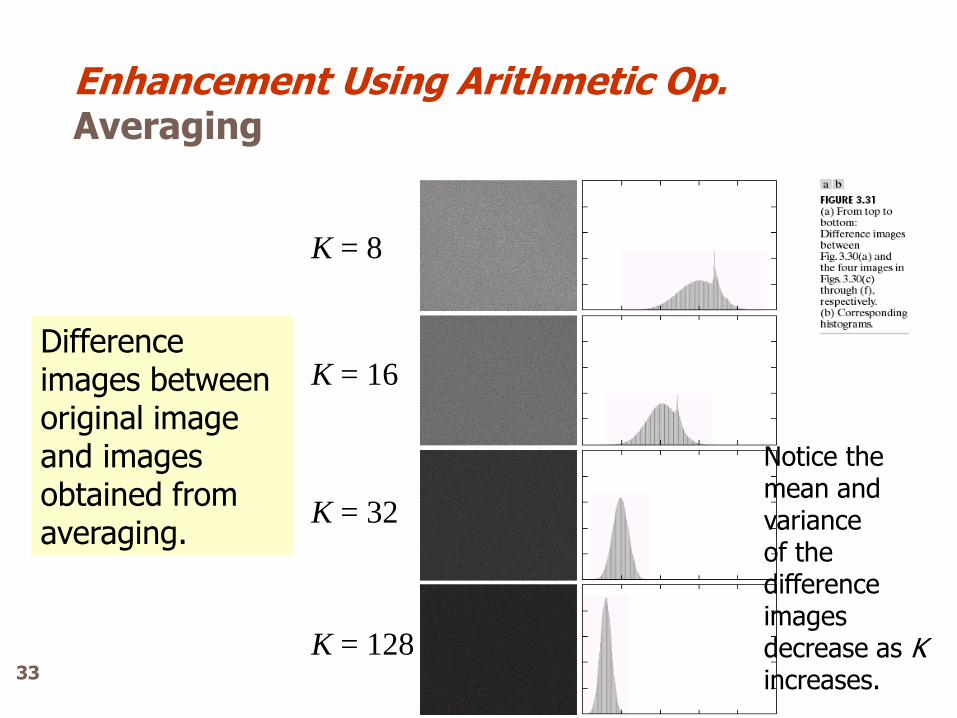
Difference images between original image and images obtained from averaging.
K = 8
K = 16
K = 32
K = 128
Notice the mean and variance of the difference images decrease as K increases.
Enhancement Using Arithmetic Op. Averaging
33
Nonlinear spatial filters operate on neighborhoods, and the mechanics of sliding a mask past an image are the same as was just outlined. In general however, the filtering operation is based conditionally on the values of the pixel in the neighborhood under consideration, and they do not explicitly use coefficients in the sum-of products manner described previously.
Example Computation for the median is a nonlinear operation.
Nonlinear of Spatial Filtering
34
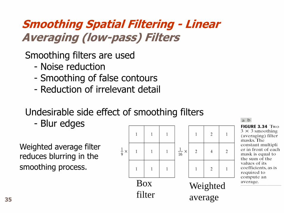
Smoothing filters are used - Noise reduction - Smoothing of false contours - Reduction of irrelevant detail Undesirable side effect of smoothing filters - Blur edges
Weighted
average
Box
filter
Weighted average filter reduces blurring in the
smoothing process.
Smoothing Spatial Filtering - Linear Averaging (low-pass) Filters
35
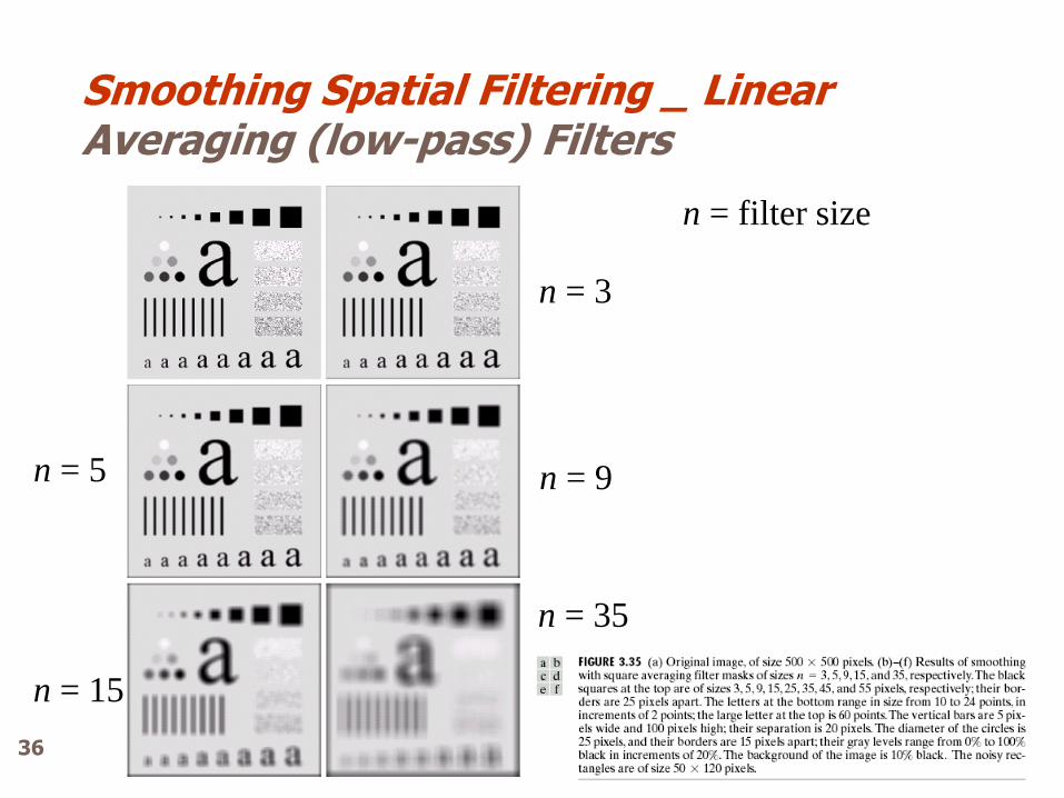
n = filter size
n = 3
n = 5 n = 9
n = 15
n = 35
Smoothing Spatial Filtering _ Linear Averaging (low-pass) Filters
36
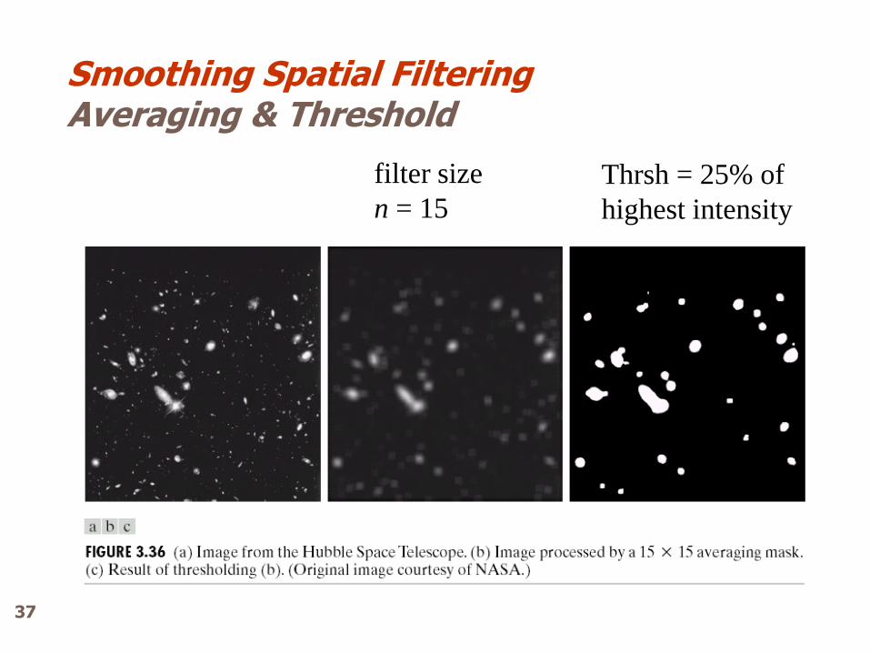
filter size
n = 15
Thrsh = 25% of
highest intensity
Smoothing Spatial Filtering Averaging & Threshold
37
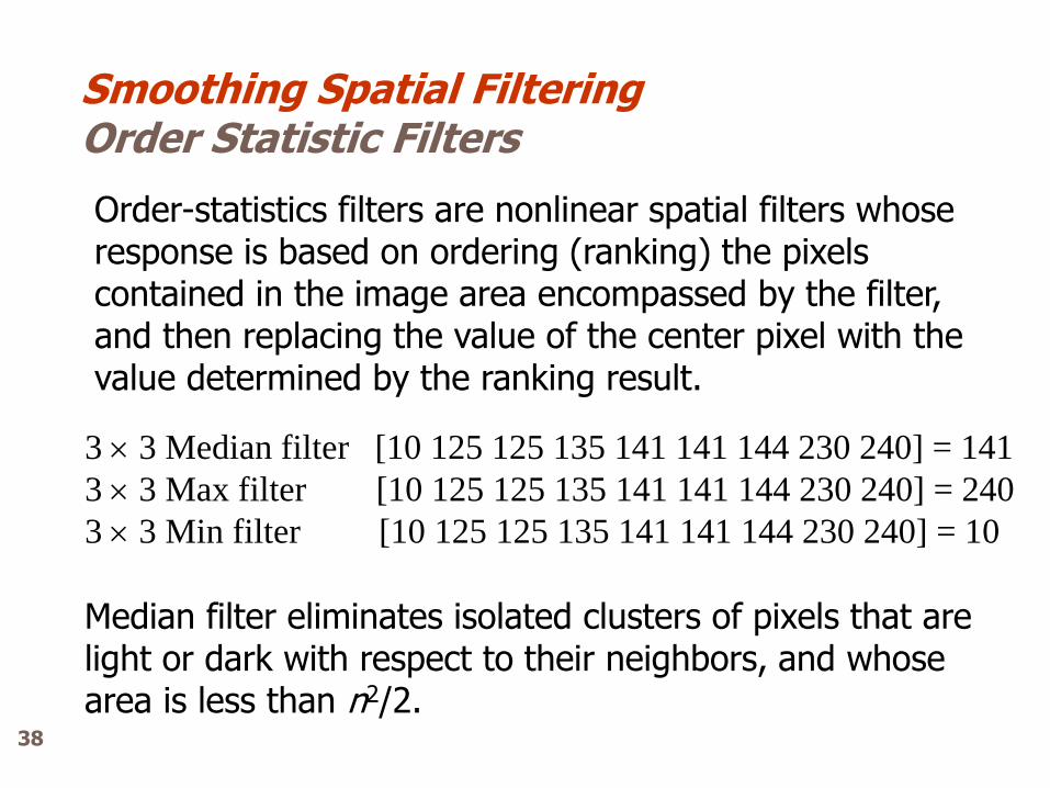
Order-statistics filters are nonlinear spatial filters whose response is based on ordering (ranking) the pixels contained in the image area encompassed by the filter, and then replacing the value of the center pixel with the value determined by the ranking result.
3 3 Median filter [10 125 125 135 141 141 144 230 240] = 141
3 3 Max filter [10 125 125 135 141 141 144 230 240] = 240
3 3 Min filter [10 125 125 135 141 141 144 230 240] = 10
Median filter eliminates isolated clusters of pixels that are light or dark with respect to their neighbors, and whose area is less than n2/2.
Smoothing Spatial Filtering Order Statistic Filters
38
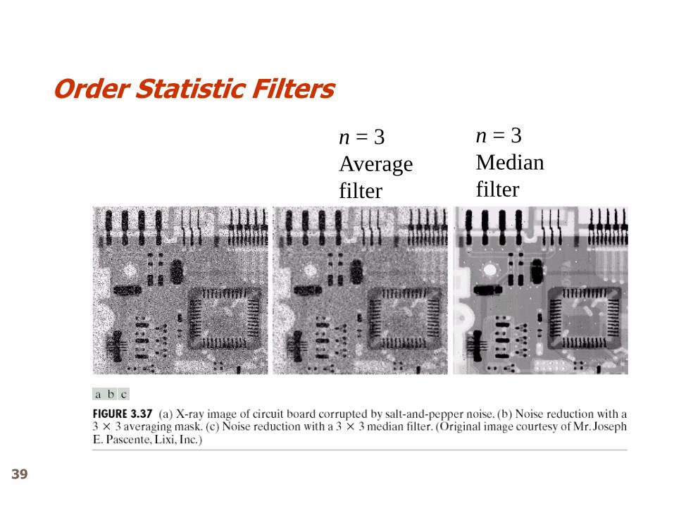
n = 3
Average
filter
n = 3
Median
filter
Order Statistic Filters
39
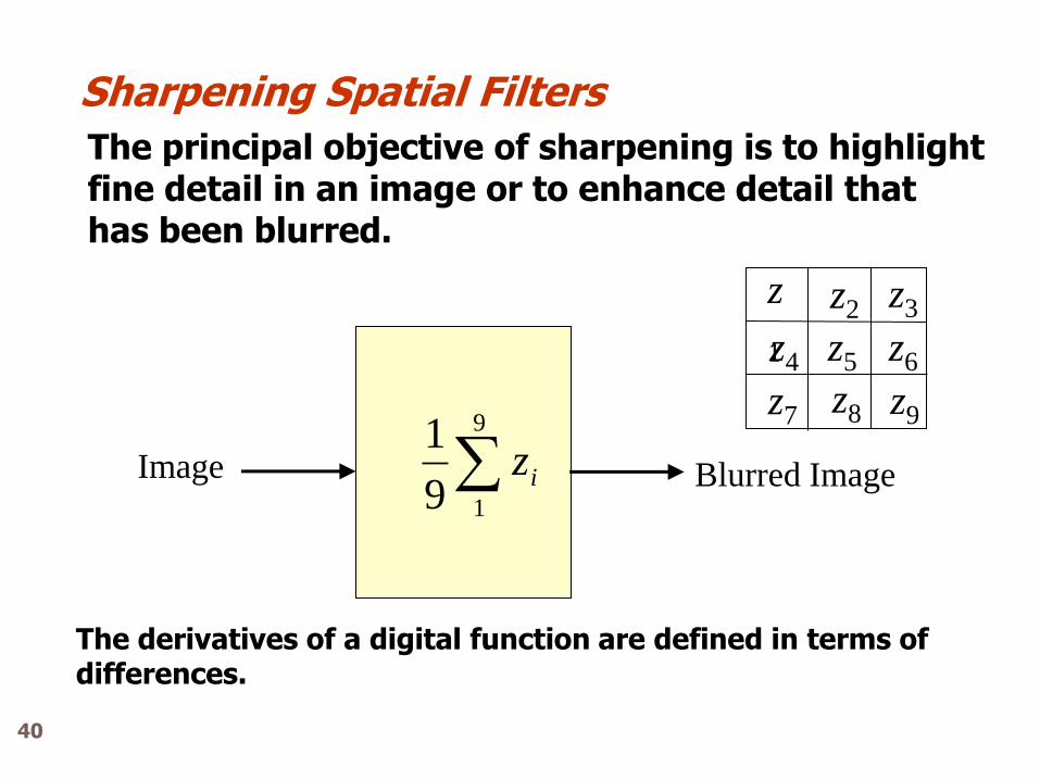
The principal objective of sharpening is to highlight fine detail in an image or to enhance detail that has been blurred.
9
19
1izImage Blurred Image
The derivatives of a digital function are defined in terms of differences.
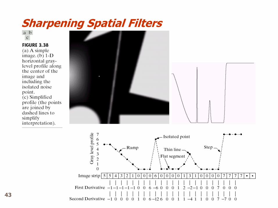
Sharpening Spatial Filters
z
1 z2
z6
z8
z4
z7
z3
z9
z5
40
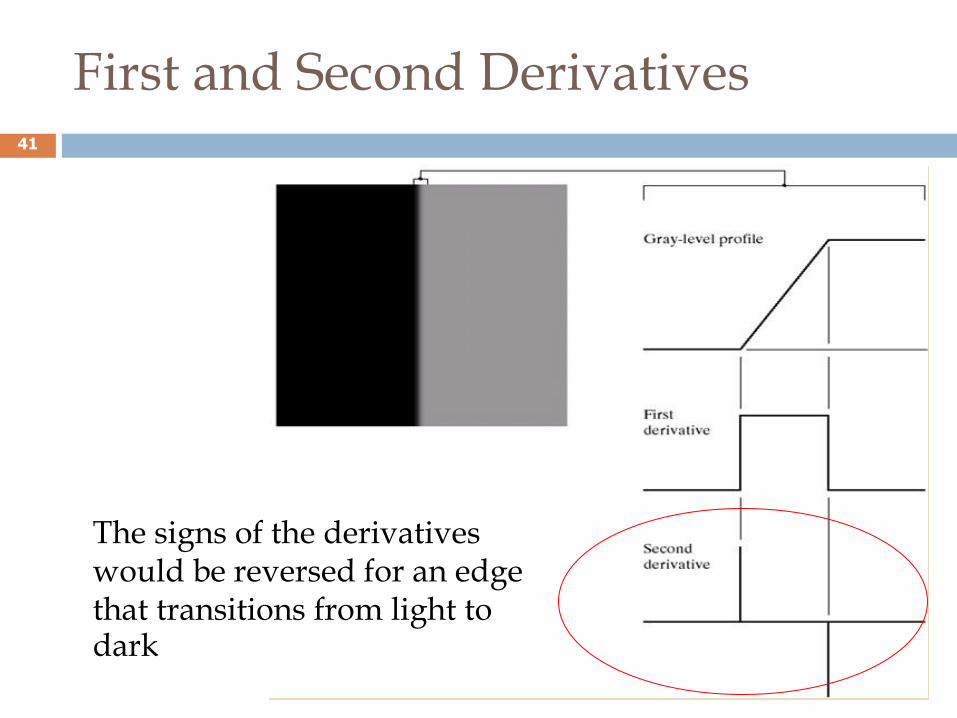
First and Second Derivatives
The signs of the derivatives would be reversed for an edge that transitions from light to dark
41
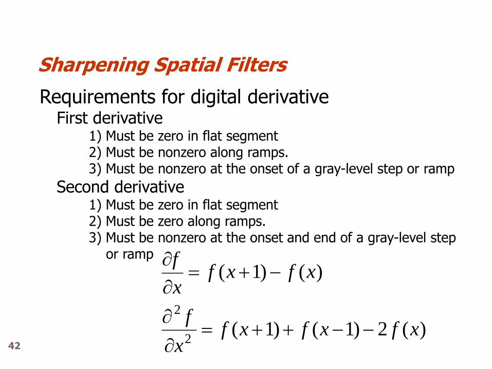
Requirements for digital derivative First derivative 1) Must be zero in flat segment 2) Must be nonzero along ramps. 3) Must be nonzero at the onset of a gray-level step or ramp
Second derivative 1) Must be zero in flat segment 2) Must be zero along ramps. 3) Must be nonzero at the onset and end of a gray-level step or ramp
)(2)1()1(
)()1(
2
2
xfxfxfx
f
xfxfx
f
Sharpening Spatial Filters
42
Sharpening Spatial Filters
43
Comparing the response between first- and second-ordered derivatives: 1) First-order derivative produce thicker edge 2) Second-order derivative have a stronger response to fine detail, such as thin lines and isolated points. 3) First-order derivatives generally have a stronger response to a gray-level step {2 4 15} 4) Second-order derivatives produce a double response at step changes in gray level.
In general the second derivative is better than the first derivative for image enhancement. The principle use of first derivative is for edge extraction.
Sharpening Spatial Filters
44
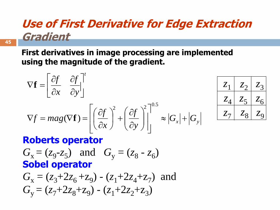
First derivatives in image processing are implemented using the magnitude of the gradient.
yx
t
GGy
f
x
fmagf
y
f
x
f
5.022
)( f
f z1 z2
z6
z8
z4
z7
z3
z9
z5
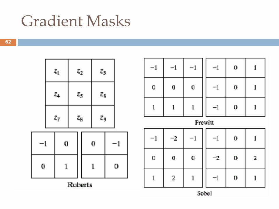
Roberts operator
Gx = (z9-z5) and Gy = (z8 - z6) Sobel operator
Gx = (z3+2z6 +z9) - (z1+2z4+z7) and
Gy = (z7+2z8+z9) - (z1+2z2+z3)
Use of First Derivative for Edge Extraction Gradient
45
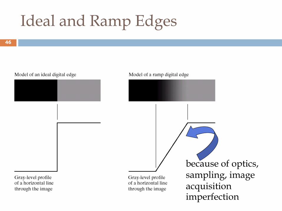
Ideal and Ramp Edges
because of optics, sampling, image acquisition imperfection
46
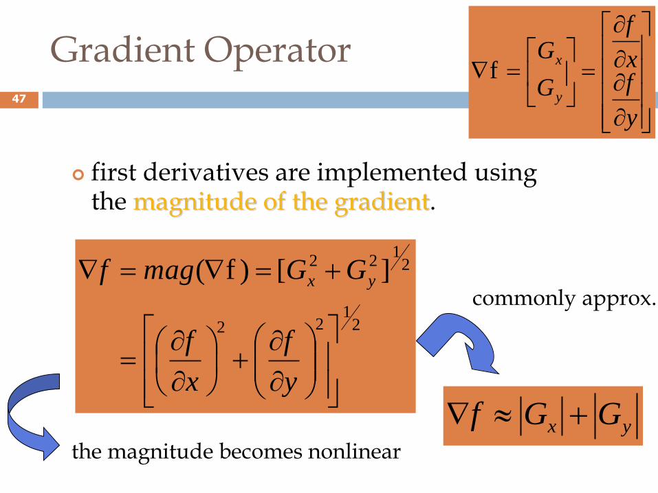
Gradient Operator
first derivatives are implemented using the magnitude of the gradient.
y
fx
f
G
G
y
xf
21
22
21
22 ][)f(
y
f
x
f
GGmagf yx
the magnitude becomes nonlinear yx GGf
commonly approx.
47
2
2
2
22
y
f
x
ff
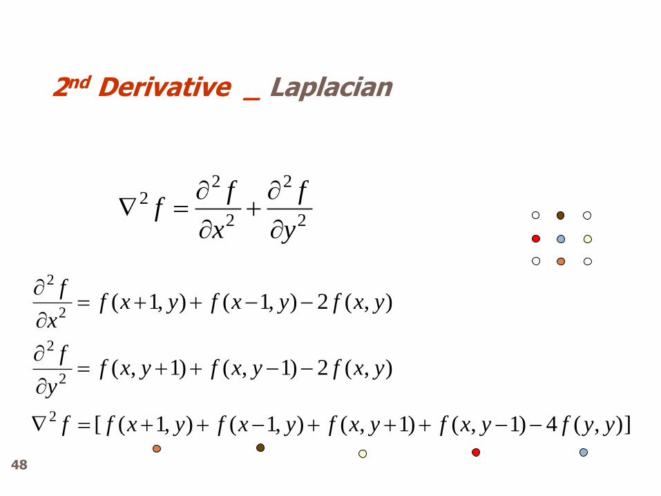
)],(4)1,()1,(),1(),1([
),(2)1,()1,(
),(2),1(),1(
2
2
2
2
2
yyfyxfyxfyxfyxff
yxfyxfyxfy
f
yxfyxfyxfx
f
2nd Derivative _ Laplacian
48
2
2
2
22
y
f
x
ff
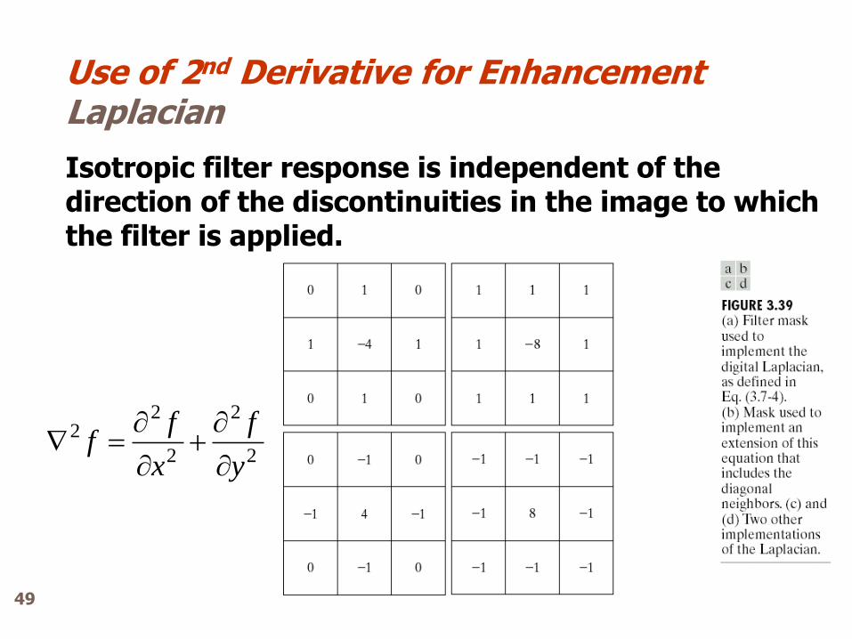
Isotropic filter response is independent of the direction of the discontinuities in the image to which the filter is applied.
Use of 2nd Derivative for Enhancement Laplacian
49
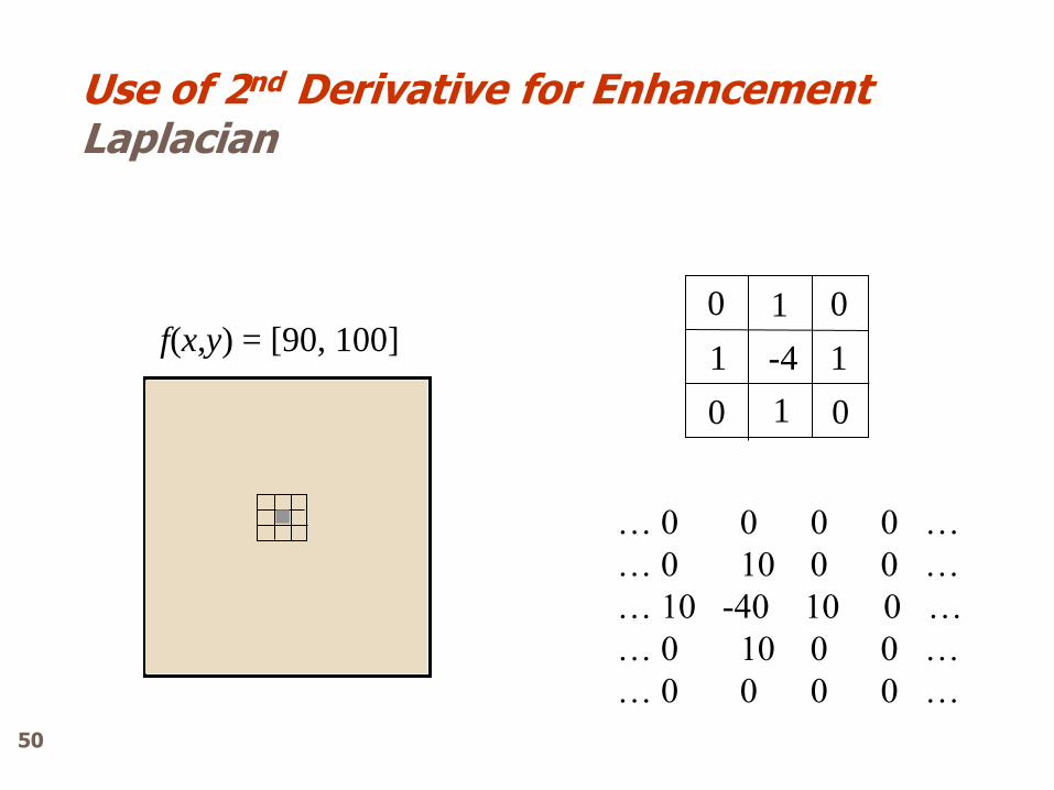
f(x,y) = [90, 100] 0 1
1
1
1
0
0
0
-4
… 0 0 0 0 …
… 0 10 0 0 …
… 10 -40 10 0 …
… 0 10 0 0 …
… 0 0 0 0 …
Use of 2nd Derivative for Enhancement Laplacian
50
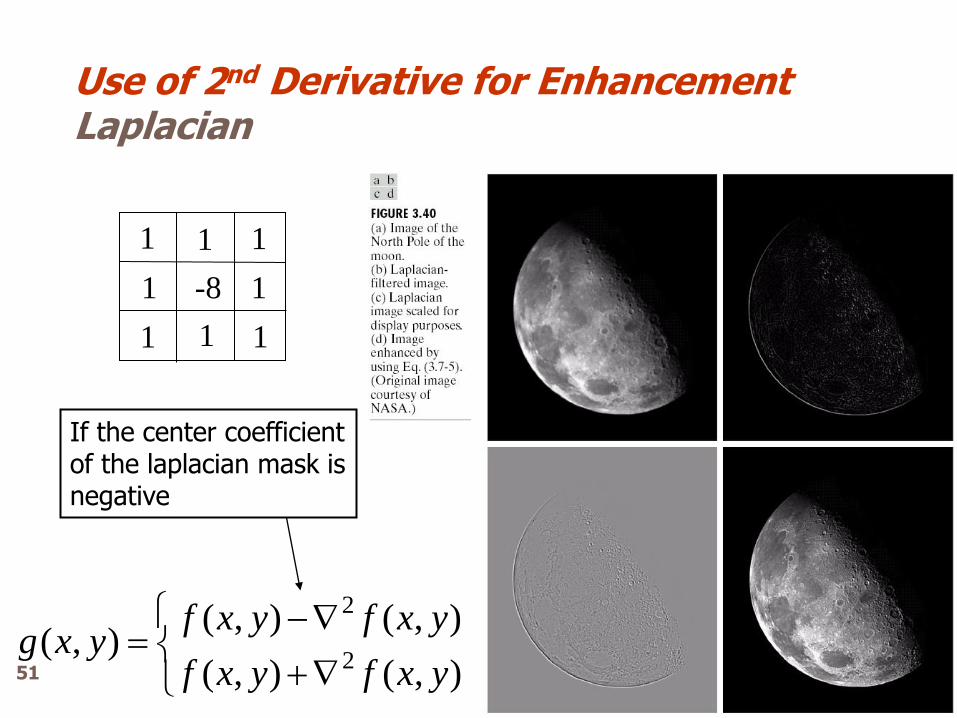
),(),(
),(),(),(
2
2
yxfyxf
yxfyxfyxg
If the center coefficient of the laplacian mask is negative
1 1
1
1
1
1
1
1
-8
Use of 2nd Derivative for Enhancement Laplacian
51
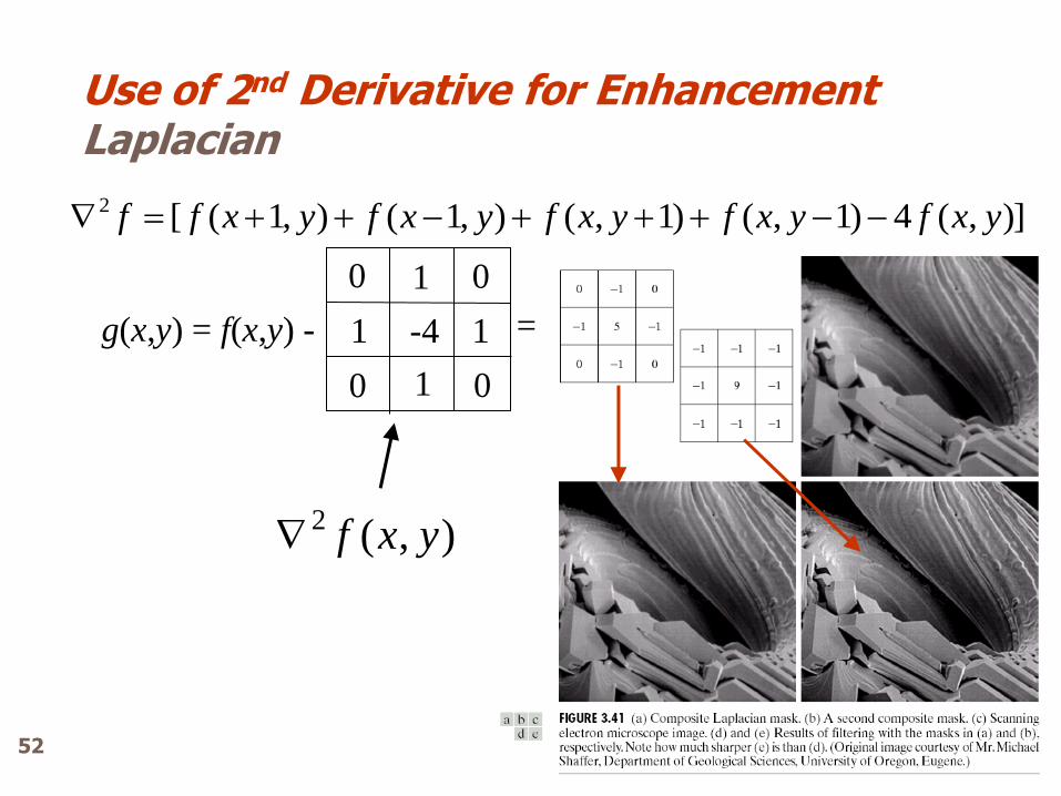
g(x,y) = f(x,y) -
0 1
1
1
1
0
0
0
-4
),(2 yxf
=
)],(4)1,()1,(),1(),1([2 yxfyxfyxfyxfyxff
Use of 2nd Derivative for Enhancement Laplacian
52
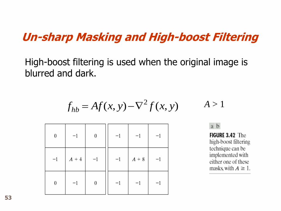
High-boost filtering is used when the original image is blurred and dark.
),(),( 2 yxfyxAffhb A > 1
Un-sharp Masking and High-boost Filtering
53
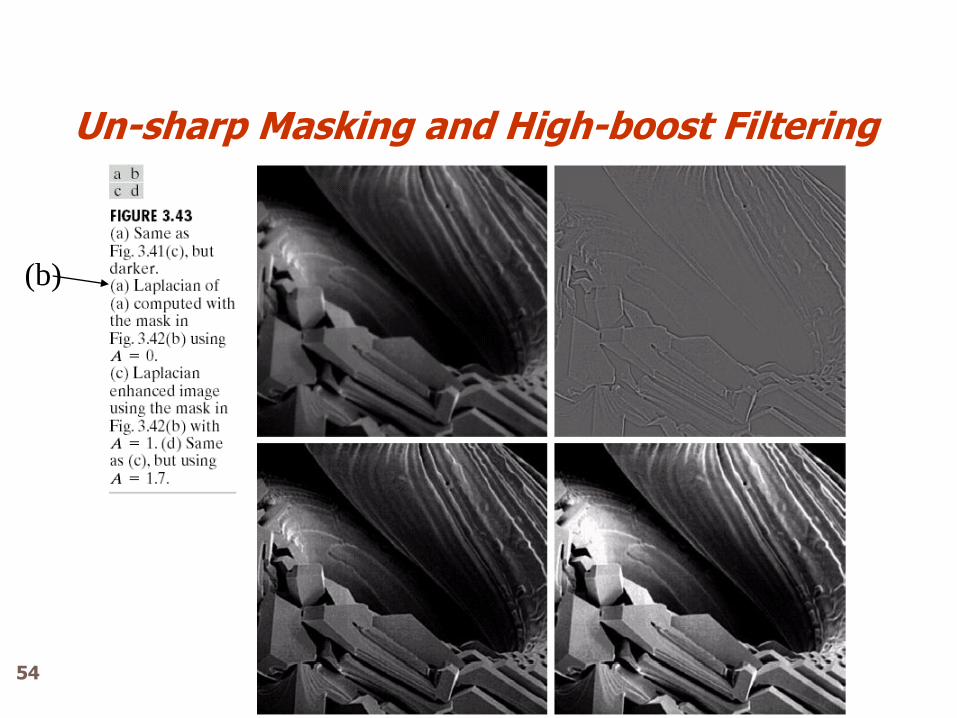
(b)
Un-sharp Masking and High-boost Filtering
54
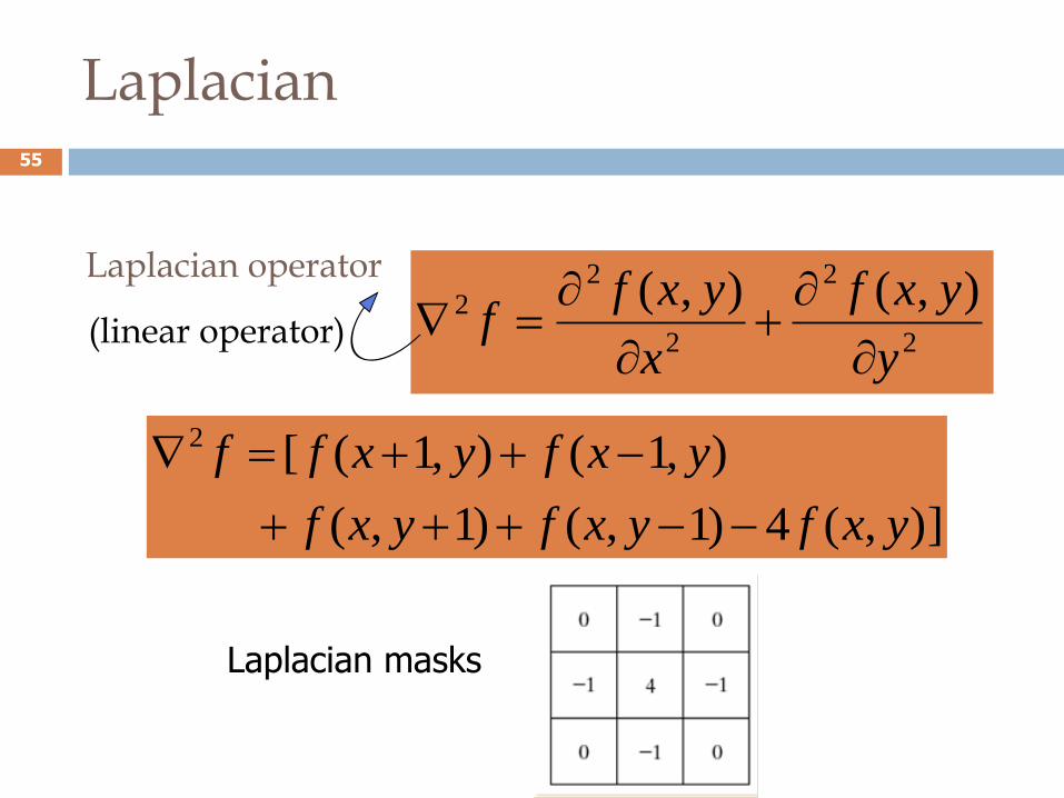
Laplacian
2
2
2
22 ),(),(
y
yxf
x
yxff
(linear operator)
Laplacian operator
)],(4)1,()1,(
),1(),1([2
yxfyxfyxf
yxfyxff
Laplacian masks
55
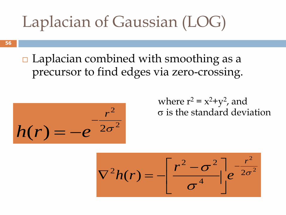
Laplacian of Gaussian (LOG)
Laplacian combined with smoothing as a precursor to find edges via zero-crossing.
2
2
2)(
r
erh
where r2 = x2+y2, and is the standard deviation
2
2
24
222 )(
r
er
rh
56
Edge detection
58
Edge Detection
Edges characterize boundaries of objects in image
A fundamental problem in image processing
Edges are areas with strong intensity contrasts
A jump in intensity from one pixel to the next
Edge detected image
Reduces significantly the amount of data,
Filters out useless information,
Preserves the important structural properties
59
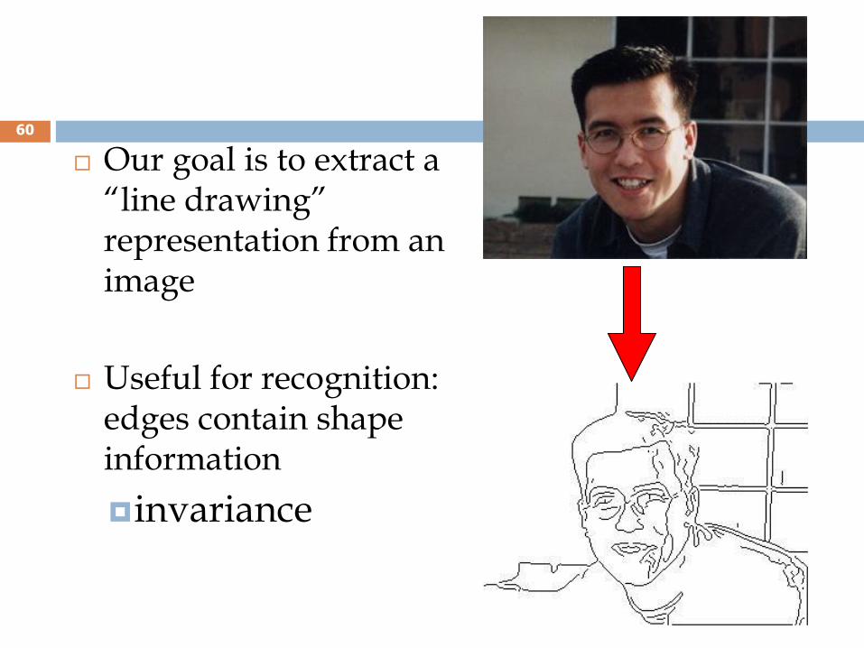
Our goal is to extract a “line drawing” representation from an image
Useful for recognition: edges contain shape information
invariance
60
Need of Edge Detection
Digital artists use it to create image outlines.
The output of an edge detector can be added back to an original image to enhance the edges
Edge detection is often the first step in image segmentation
Edge detection is also used in image registration by alignment of two images that may have been acquired at separate times or from different sensors
61
Gradient Masks
62
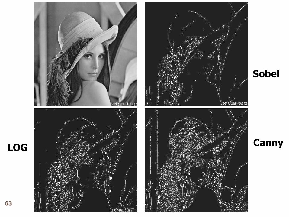
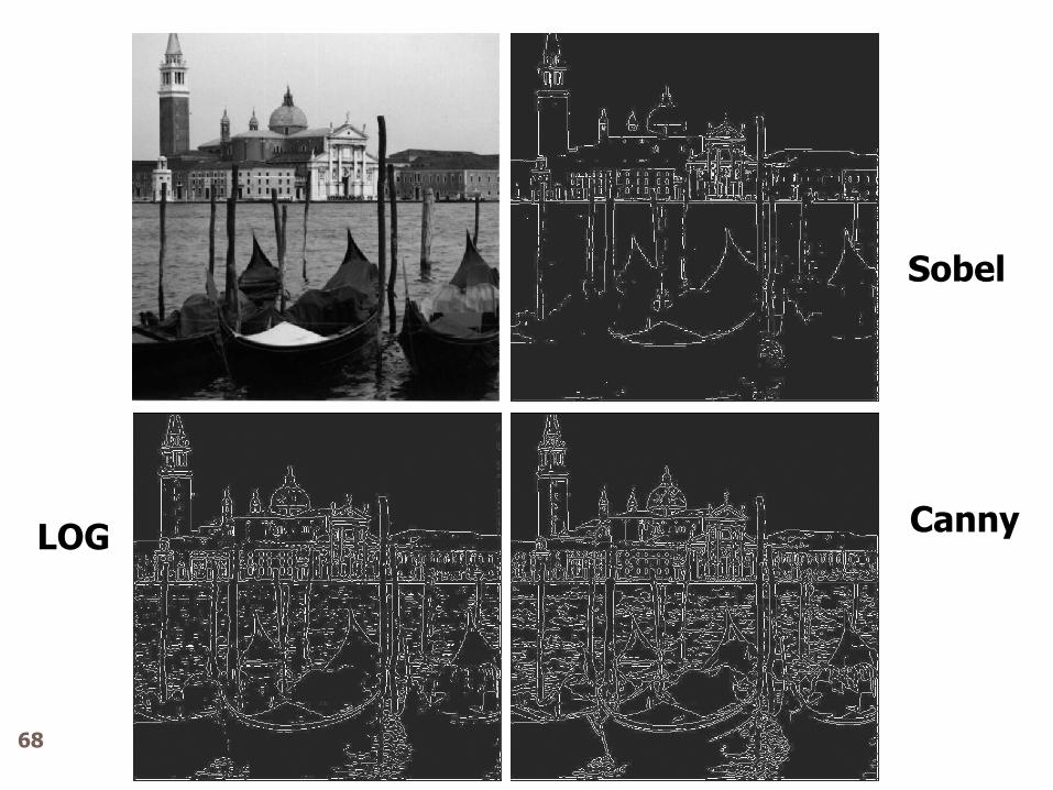
Sobel
Canny LOG
63
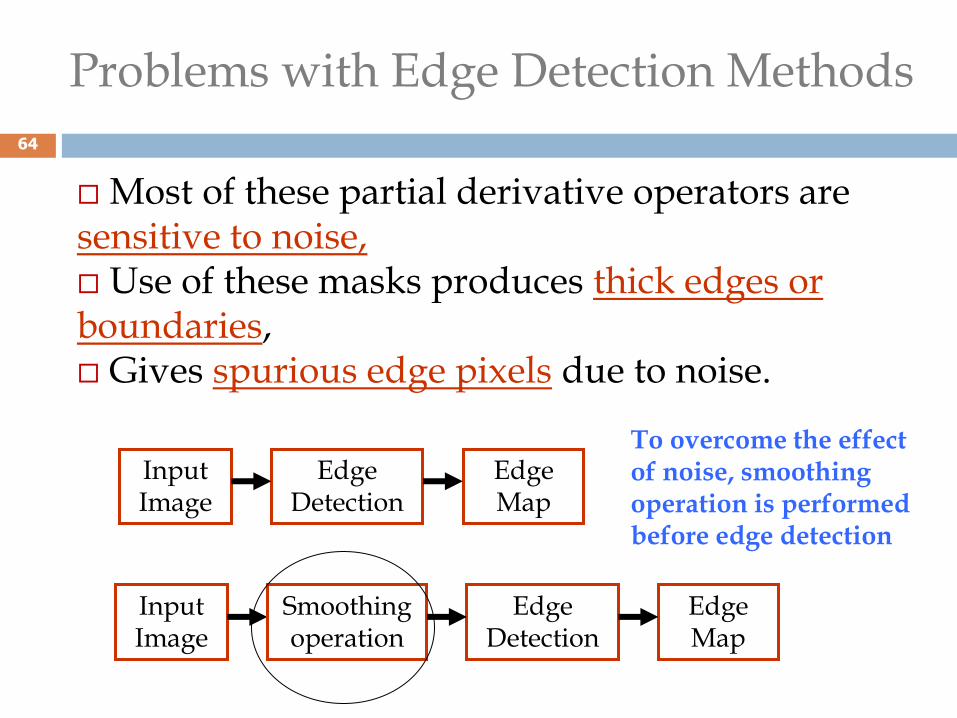
Most of these partial derivative operators are sensitive to noise, Use of these masks produces thick edges or boundaries, Gives spurious edge pixels due to noise.
Problems with Edge Detection Methods
To overcome the effect of noise, smoothing operation is performed before edge detection
Edge Detection
Input Image
Edge Map
Edge Detection
Input Image
Edge Map
Smoothing operation
64
Smoothing based Edge Detection
Two operators which use smoothing
Marr-Hildreth operator
Laplacian of Gaussian function (LOG)
Follows 2-Operations
Smoothing
Applying Laplacian operator
Or generate the combined mask of LOG
Canny Edge Detector
65
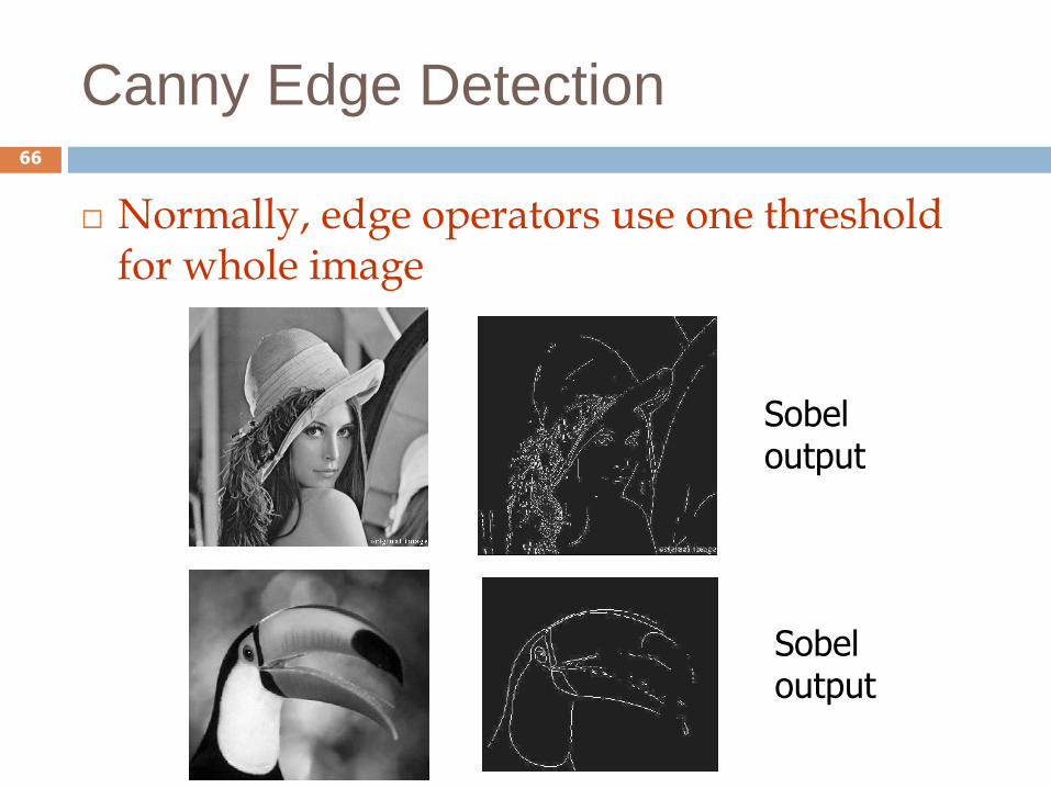
Canny Edge Detection
Normally, edge operators use one threshold for whole image
Sobel output
Sobel output
66
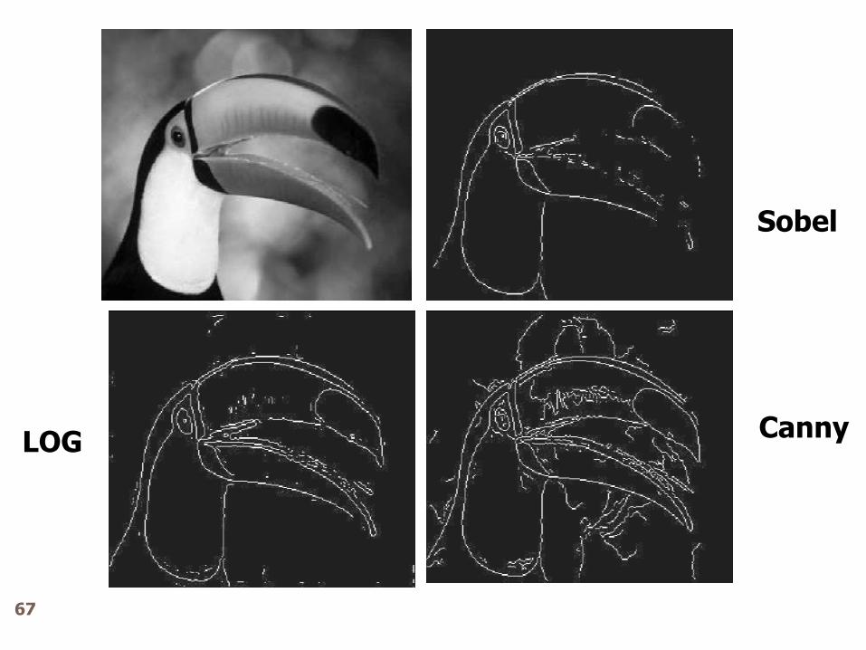
Sobel
Canny LOG
67
Sobel
Canny LOG
68
Canny Edge Detector (J. Canny’
1986):
An "optimal" edge detector means:
Good detection - the algorithm should mark as many real edges in the image as possible.
Good localization - edges marked should be as close as possible to the edge in the real image.
Canny edge detector uses two threshold values to detect weak and strong edges
69

Frequency Domain Filtering
70
2/122
1
0
1
0
)(2
1
0
1
0
)(2
),(),(),(
),(),(
),(1
),(
vuIvuRvuF
evuFyxf
eyxfMN
vuF
M
u
N
v
yN
vx
M
uj
M
x
N
y
N
yv
M
xuj
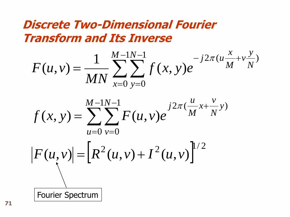
Fourier Spectrum
Discrete Two-Dimensional Fourier Transform and Its Inverse
71
1
0
1
0
),(1
)0,0(M
x
N
y
yxfMN
F
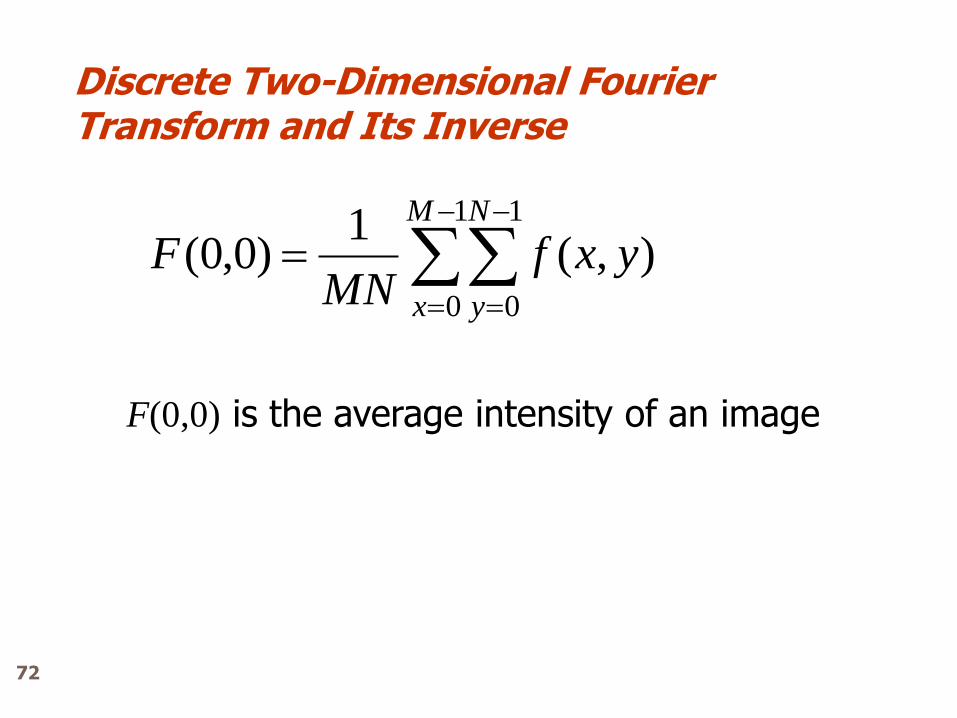
F(0,0) is the average intensity of an image
Discrete Two-Dimensional Fourier Transform and Its Inverse
72
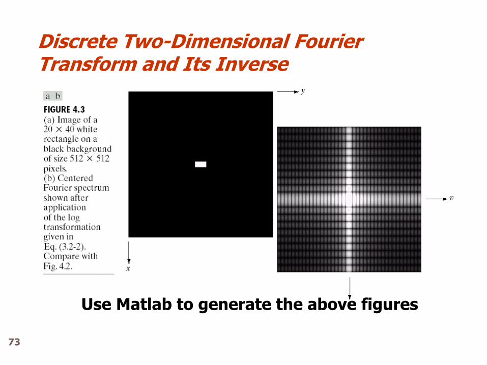
Use Matlab to generate the above figures
Discrete Two-Dimensional Fourier Transform and Its Inverse
73


![Corso Completo Javascript - Grimaldi Group · [unità2] - HTML.IT - Corso Completo JavaScript La nascita di Javascript Il World Wide Web si è sviluppato grazie alla possibilità](https://static.fdocuments.pl/doc/165x107/5ad35d587f8b9a0f198d8d2b/corso-completo-javascript-grimaldi-unit2-htmlit-corso-completo-javascript.jpg)