
AnthropologicAl AnAlysis of ZlotA culture skeletons from ...
Projekt współfinansowany ze środków Unii Europejskiej w ramach Europejskiego Funduszu Społecznego
ROZWÓJ POTENCJAŁU I OFERTY DYDAKTYCZNEJ POLITECHNIKI WROCŁAWSKIEJ
Wrocław University of Technology
Computer Engineering
Krzysztof Brzostowski, Jarosław Drapała
SYSTEMS MODELLING
AND ANALYSIS
Wrocław 2011
Wrocław University of Technology
Computer Engineering
Krzysztof Brzostowski, Jarosław Drapała
SYSTEMS MODELLING
AND ANALYSIS Advanced Technology in Electrical Power Generation
Wrocław 2011

Reviewer
Jerzy Świątek
Project Office
ul. M. Smoluchowskiego 25, room 407
50-372 Wrocław, Poland
Phone: +48 71 320 43 77
Email: [email protected]
Website: www.studia.pwr.wroc.pl

Contents
1. Dynamic Systems Modelling and Analysis ...................................................................................... 5
1.1. Differential Equation ............................................................................................................... 5
1.2. State Vector Description ....................................................................................................... 10
1.3. Transfer Function .................................................................................................................. 16
1.4. Linear Systems Analysis ......................................................................................................... 24
1.5. Nonlinear Systems Analysis ................................................................................................... 28
2. Identification ................................................................................................................................. 32
2.1 Determination of the System Parameters ............................................................................ 33
2.2. The choice of the Best Model: Deterministic Case ............................................................... 40
2.3 Parameter Estimation of the System’s Characteristic ........................................................... 51
2.4 The choice of the Best Model: Probabilistic Case ................................................................. 65
2.5 Example Application of the System Identification for Real Life Problem ............................. 71
Bibliography ........................................................................................................................................... 75
5
1. Dynamic Systems Modelling and Analysis
1.1. Differential Equation
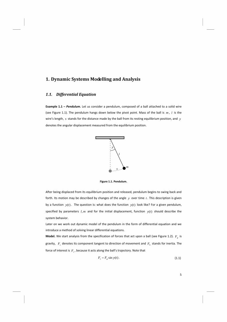
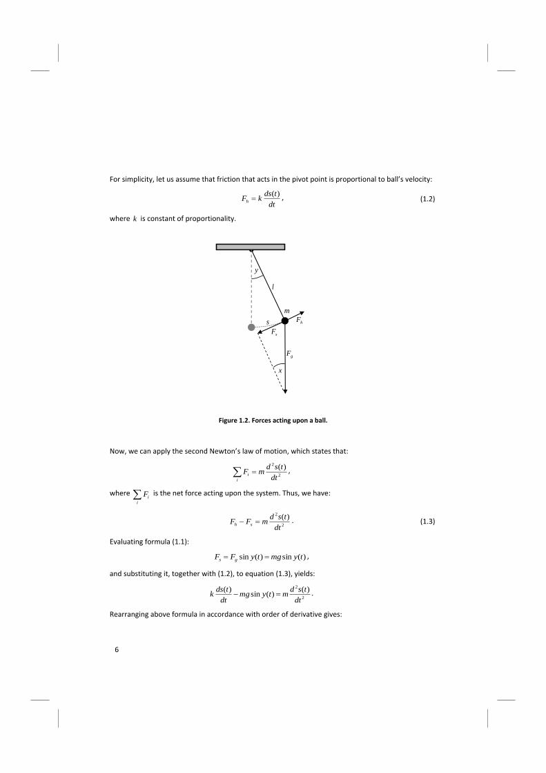
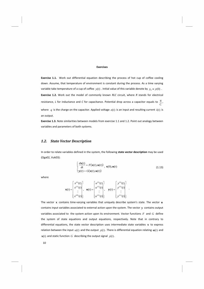
Example 1.1 – Pendulum. Let us consider a pendulum, composed of a ball attached to a solid wire
(see Figure 1.1). The pendulum hangs down below the pivot point. Mass of the ball is m , l is the
wire’s length, s stands for the distance made by the ball from its resting equilibrium position, and y
denotes the angular displacement measured from the equilibrium position.
After being displaced from its equilibrium position and released, pendulum begins to swing back and
forth. Its motion may be described by changes of the angle y over time t . This description is given
by a function )(ty . The question is: what does the function )(ty look like? For a given pendulum,
specified by parameters ml, and for the initial displacement, function )(ty should describe the
system behavior.
Later on we work out dynamic model of the pendulum in the form of differential equation and we
introduce a method of solving linear differential equations.
Model. We start analysis from the specification of forces that act upon a ball (see Figure 1.2). gF is
gravity, sF denotes its component tangent to direction of movement and
hF stands for inertia. The
force of interest is sF , because it acts along the ball’s trajectory. Note that
)(sin tyFF gs . (1.1)
l
m s
y
Figure 1.1. Pendulum.
6
For simplicity, let us assume that friction that acts in the pivot point is proportional to ball’s velocity:
dt
tdskFh
)( , (1.2)
where k is constant of proportionality.
Now, we can apply the second Newton’s law of motion, which states that:
2
2 )(
dt
tsdmF
i
i ,
where i
iF is the net force acting upon the system. Thus, we have:
2
2 )(
dt
tsdmFF sh . (1.3)
Evaluating formula (1.1):
)(sin)(sin tymgtyFF gs ,
and substituting it, together with (1.2), to equation (1.3), yields:
2
2 )()(sin
)(
dt
tsdmtymg
dt
tdsk .
Rearranging above formula in accordance with order of derivative gives:
s
l
m
x
hF
gF
sF
y
Figure 1.2. Forces acting upon a ball.
7
0)(sin)()(
2
2
tygdt
tds
m
k
dt
tsd . (1.4)
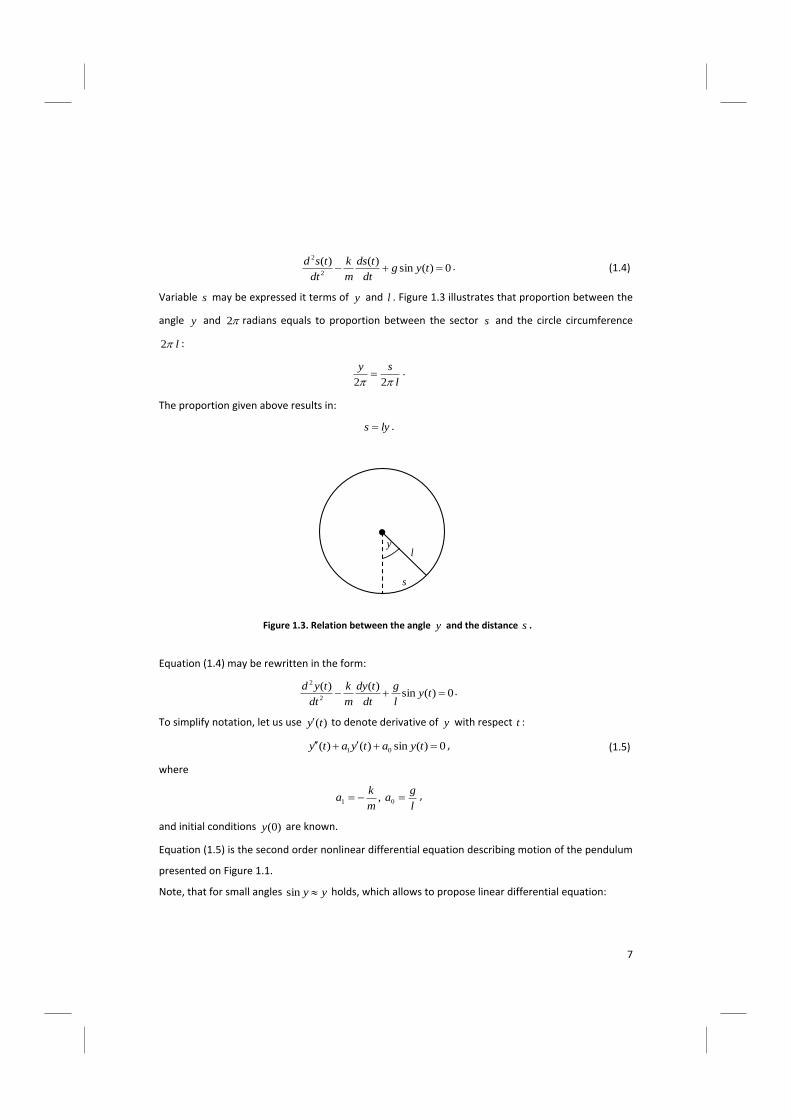
Variable s may be expressed it terms of y and l . Figure 1.3 illustrates that proportion between the
angle y and 2 radians equals to proportion between the sector s and the circle circumference
l2 :
l
sy
22 .
The proportion given above results in:
lys .
Equation (1.4) may be rewritten in the form:
0)(sin)()(
2
2
tyl
g
dt
tdy
m
k
dt
tyd .
To simplify notation, let us use )(ty to denote derivative of y with respect t :
0)(sin)()( 01 tyatyaty , (1.5)
where
l
ga
m
ka 01 , ,
and initial conditions )0(y are known.
Equation (1.5) is the second order nonlinear differential equation describing motion of the pendulum
presented on Figure 1.1.
Note, that for small angles yy sin holds, which allows to propose linear differential equation:
y
l
s
Figure 1.3. Relation between the angle y and the distance s .
8
0)()()( 01 tyatyaty . (1.6)
This equations describes the system behavior only for small displacements from the resting position.
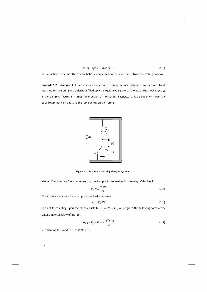
Example 1.2 – Damper. Let us consider a forced mass-spring-damper system, composed of a block
attached to the spring and a dashpot filled up with liquid (see Figure 1.4). Mass of the block is m ,
is the damping factor, k stands for modulus of the spring elasticity, y is displacement from the
equilibrium position and u is the force acting on the spring.
Model. The damping force generated by the dashpot is proportional to velocity of the block:
dt
tdyF
)( . (1.7)
The spring generates a force proportional to displacement:
)(tykFk . (1.8)
The net force acting upon the block equals to kFFtu )( , which gives the following form of the
second Newton’s law of motion:
2
2 )()(
dt
tydmFFtu k
. (1.9)
Substituting (1.7) and (1.8) to (1.9) yields:
m
k
)(tu
)(ty
Figure 1.4. Forced mass-spring-damper system.
9
2
2 )()(
)()(
dt
tydmtky
dt
tdytu ,
and applying )()(
tydt
tdy :
)()()()( tutkytytym .
Dividing both sides by m gives:
)(1
)()()( tum
tym
kty
mty
.
Denoting:
mb
m
ka
ma
1,, 001
,
We obtain the second order differential equation:
)()()()( 001 tubtyatyaty . (1.10)
Compare models (1.6) and (1.10). The first model describes linearized unforced system, but left sides
of equations are identical. For )(0)( ttu both models are identical. Different physical objects have
similar description, which means that variables of both systems are related in the same way.
Therefore, analysis made on the model (1.10) applies for all possible systems that may be described
by this equation. Another example of the system with description (1.10) is RLC circuit. Interpretation
of variables is different, but model remains the same.
In general, differential equation is equation of the form (Bro06, Oga02):
0)(,)(
,,)(
,)(
);(,)(
,,)(
,)(
1
1
1
1
tudt
tdu
dt
tud
dt
tudty
dt
tdy
dt
tyd
dt
tydf
v
v
v
v
m
m
m
m
. (1.11)
Linear differential equation is particular example of the above equation:
,)()()()(
)()()()(
011
1
1
011
1
1
tubdt
tdub
dt
tudb
dt
tudb
tyadt
tdya
dt
tyda
dt
tyd
v
v
vv
v
v
m
m
mm
m
(1.12)
where vm holds.
10
Exercises
Exercise 1.1. Work out differential equation describing the process of hot cup of coffee cooling
down. Assume, that temperature of environment is constant during the process. As a time varying
variable take temperature of a cup of coffee )(ty . Initial value of this variable denote by )0(0 yy .
Exercise 1.2. Work out the model of commonly known RLC circuit, where R stands for electrical
resistance, L for inductance and C for capacitance. Potential drop across a capacitor equals to C
q ,
where q is the charge on the capacitor. Applied voltage )(te is an input and resulting current )(ti is
an output.
Exercise 1.3. Note similarities between models from exercise 1.1 and 1.2. Point out analogy between
variables and parameters of both systems.
1.2. State Vector Description
In order to relate variables defined in the system, the following state vector description may be used
(Oga02, Vuk03):
)(),()(
)(),()(
ttGt
ttFdt
td
uxy
uxx
, )(),0( tux (1.13)
where
)(
)(
)(
)(,
)(
)(
)(
)(,
)(
)(
)(
)(
)(
)2(
)1(
)(
)2(
)1(
)(
)2(
)1(
ty
ty
ty
t
tu
tu
tu
t
tx
tx
tx
t
LSR
yux .
The vector x contains time-varying variables that uniquely describe system’s state. The vector u
contains input variables associated to external action upon the system. The vector y contains output
variables associated to the system action upon its environment. Vector functions F and G define
the system of state equations and output equations, respectively. Note that in contrary to
differential equations, the state vector description uses intermediate state variables x to express
relation between the input )(tu and the output )(ty . There is differential equation relating )(tu and
)(tx and static function G describing the output signal )(ty .
11
State equations have form:
)(,),(),();(,),(),()(
)(,),(),();(,),(),()(
)(,),(),();(,),(),()(
)()2()1()()2()1()(
)()2()1()()2()1(
2
)2(
)()2()1()()2()1(
1
)1(
tutututxtxtxfdt
tdx
tutututxtxtxfdt
tdx
tutututxtxtxfdt
tdx
SR
R
R
SR
SR
,
and output equations have form:
)(,),(),();(,),(),()(
)(,),(),();(,),(),()(
)(,),(),();(,),(),()(
)()2()1()()2()1()(
)()2()1()()2()1(
2
)2(
)()2()1()()2()1(
1
)1(
tutututxtxtxgty
tutututxtxtxgty
tutututxtxtxgty
SR
L
L
SR
SR
.
Linear system is described by a particular form of state vector description (1.13):
)()()(
)()()(
ttt
ttdt
td
DuCxy
BuAxx
, (1.14)
where DCBA ,,, are matrices of the form: SLRLSRRR RRRR DCBA ,,, .
Example 1.3 – Damper. Let us take differential equation (1.10) describing behavior of the forced
spring-mass-damper system. In order to describe it by state vector description, we introduce two
state variables:
dt
tdxtx
txtx
)()(
)()(
)2(
)1(
.
Variable )1(x stands for displacement and )2(x is velocity. These two time varying variables give full
information about the current state of the system. Now, we work out state vector description on the
basis of differential equation (1.10). It is required to find formulas for dt
tdx )()1(
and dt
tdx )()2(
as
relations involving )1(x , )2(x and system parameters. The first formula is a consequence of state
variable definition:
12
)()()( )2(
)1(
txdt
tdx
dt
tdx .
The second formula is derived from (1.10):
)()()()(
0
)1(
0
)1(
1
)2(
tubtxadt
tdxa
dt
tdx ,
which gives:
)()()()(
0
)2(
1
)1(
0
)2(
tubtxatxadt
tdx .
As the output we decide to take )()( )1()1( txty .
Eventually, we obtain state vector description in the form:
)()(
)(1
)()()(
)()(
)1(
)2()1()2(
)2()1(
txty
tum
txm
txm
k
dt
tdx
txdt
tdx
. (1.15)
Equivalent matrix representation has the form:
)(01)(
)(1
0)(
10)(
tt
tum
tmmkdt
td
xy
xx
. (1.16)
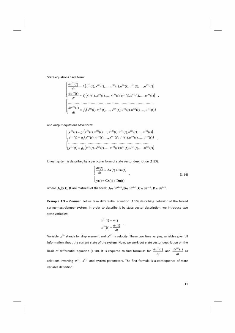
Example 1.4 – State vector description and SIMULINK. On the basis of state vector description it is
easy to implement the system model in SIMULINK environment, which is a part of MATLAB software.
Implementation of state vector (1.15) is illustrated in Figure 1.5.
The model is composed of pre-defined building blocks representing mathematical operations. Blocks
labeled by s
1 are integrators and they integrate input value over time, beginning from the initial
value, up to the total simulation time. Initial values are set up in the block’s parameters window.
Outputs of these two blocks are values of )()1( tx and )()2( tx at the time t solved numerically by
Runge-Kutty method (Bro06). Another blocks allow to define constant parameters: square blocks
with no inputs give constant value as output (‘m’ is 2m ), triangle blocks are constant gains (‘k’ is
1.1k and ‘mu’ is 2.1 ).
13
There are also blocks that do summation, division, and multiplication (the ‘product’ block). The
‘clock’ block returns current time t . The group of blocks on the bottom left implement input signal
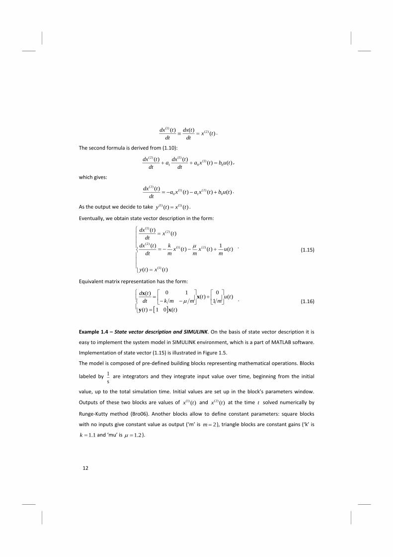
tetu t sin)( 1.0 . Output signals )()1( tx and )()2( tx are illustrated in Figure 1.6.
Figure 1.5. SIMULINK implementation of a forced mass-spring-damper system model.
Figure 1.6. Solution of the model for initial conditions 0)0(,3)0( )2()1( xx .
Another view on the solution is given on the so called phase plane (see Figure 1.7) where axis stand
for state variables.
14
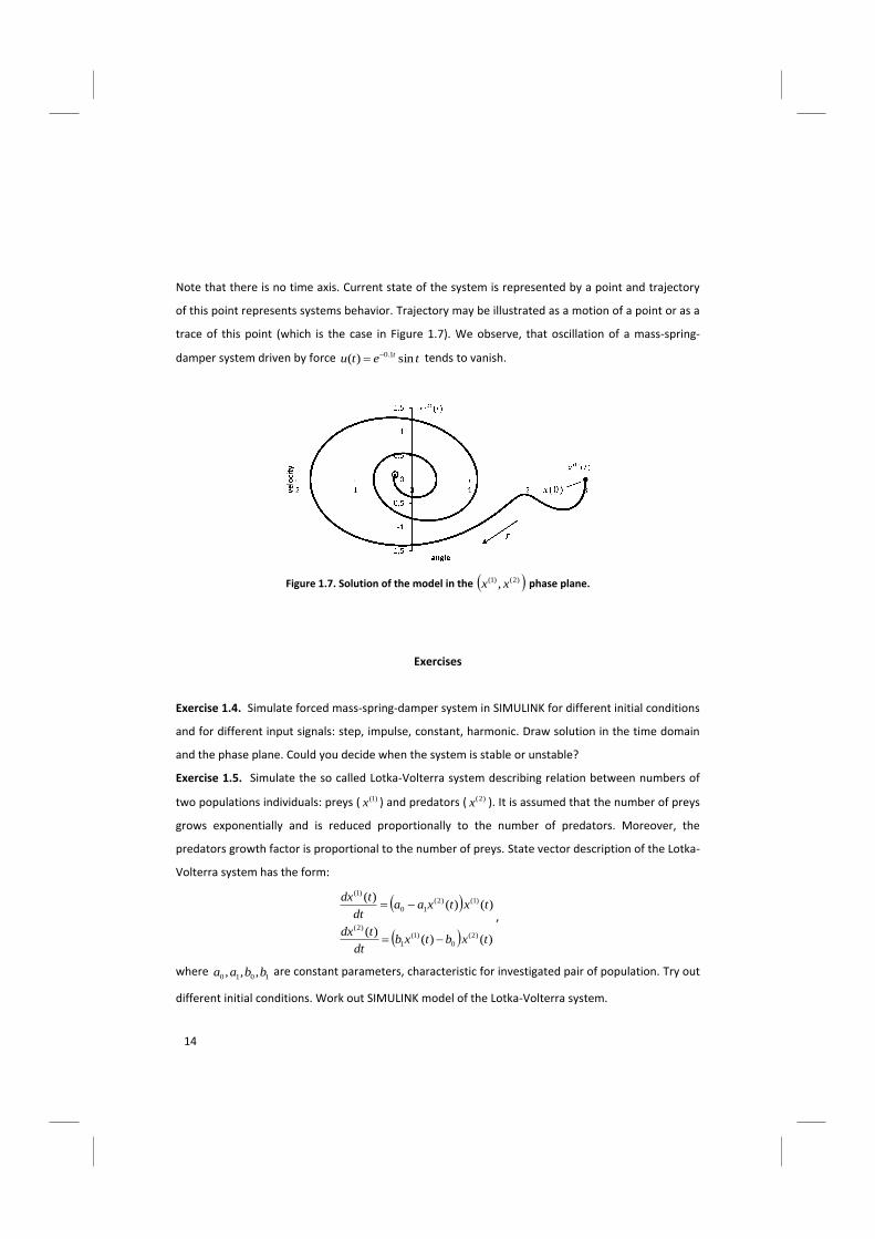
Note that there is no time axis. Current state of the system is represented by a point and trajectory
of this point represents systems behavior. Trajectory may be illustrated as a motion of a point or as a
trace of this point (which is the case in Figure 1.7). We observe, that oscillation of a mass-spring-
damper system driven by force tetu t sin)( 1.0 tends to vanish.
Figure 1.7. Solution of the model in the )2()1( , xx phase plane.
Exercises
Exercise 1.4. Simulate forced mass-spring-damper system in SIMULINK for different initial conditions
and for different input signals: step, impulse, constant, harmonic. Draw solution in the time domain
and the phase plane. Could you decide when the system is stable or unstable?
Exercise 1.5. Simulate the so called Lotka-Volterra system describing relation between numbers of
two populations individuals: preys ( )1(x ) and predators ( )2(x ). It is assumed that the number of preys
grows exponentially and is reduced proportionally to the number of predators. Moreover, the
predators growth factor is proportional to the number of preys. State vector description of the Lotka-
Volterra system has the form:
)()()(
)()()(
)2(
0
)1(
1
)2(
)1()2(
10
)1(
txbtxbdt
tdx
txtxaadt
tdx
,
where 1010 ,,, bbaa are constant parameters, characteristic for investigated pair of population. Try out
different initial conditions. Work out SIMULINK model of the Lotka-Volterra system.
15
For different values of parameters and initial conditions analyze its behavior on the time domain and
the phase plane. Does the system have any equilibrium states?
Exercise 1.6. Simulate the human heart dynamics using the Zeeman model of the form:
btxdt
tdx
txtxtaxdt
tdx
)()(
)()()()(
)1()2(
3)1()2()1()1(
,
where )1(x denotes length of heart’s muscle fibers, )2(x is electrochemical stimulus’ strength, a
stands for effect of blood pressure and parameter b determines position of the equilibrium point.
Implement Zeeman model in SIMULINK. Analyze its behavior in the time domain and on the phase
plane, trying different initial conditions. Can you observe the so called limit cycle? Simulate the
system for different values of parameter a : 0a , small value of 0a , high value of 0a , and
different values of parameter b : 3ab and 3ab . On the ba, parameters plane draw
areas where the system is stable and unstable.
Exercise 1.7. A simplified model of the weather behavior proposed by Lorenz has the form:
)()(
)()(
)()()(
)3()2()1()3(
)3()1()2()1()2(
)1()2()1(
txxxdt
tdx
xxxtxdt
tdx
txtxdt
tdx
,
where )1(x is velocity of the air ascendance, )2(x is the difference between ascendant and
descendant air columns temperatures, )3(x is a measure of deviation of )()2( tx over time from
linearity, ,, are constant parameters. Work out SIMULINK model of the Lorenz system taking:
38,28,10 . Analyze its behavior in the time domain and on the phase plane. How to
visualize three dimensional trajectory covered by the system? Compare two trajectories with slightly
different initial positions. Do they stay close to each other as long as time goes by? Try also to
analyze the system with 170,145 .
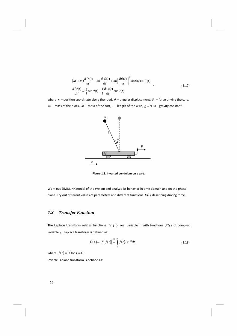
Exercise 1.8. Work out state vector description for inverted pendulum on a cart (see Figure 1.8),
described by following set of differential equations:
16
)(cos)(1
)(sin)(
)()(sin)()()(
2
2
2
2
2
2
2
2
2
tdt
txd
lt
l
g
dt
td
tFtdt
tdml
dt
tdml
dt
txdmM
, (1.17)
where x – position coordinate along the road, – angular displacement, F – force driving the cart,
m – mass of the block, M – mass of the cart, l – length of the wire, 81.9g – gravity constant.
Work out SIMULINK model of the system and analyze its behavior in time domain and on the phase
plane. Try out different values of parameters and different functions )(tF describing driving force.
1.3. Transfer Function
The Laplace transform relates functions )(tf of real variable t with functions )(sF of complex
variable s . Laplace transform is defined as:
o
stdtetftfsFdf
L , (1.18)
where 0tf for 0t .
Inverse Laplace transform is defined as:
F
l
m
x
M
Figure 1.8. Inverted pendulum on a cart.
17
jc
jc
stdsesFj
sFtf2
1df1L . (1.19)
Example 1.5 – Working out Laplace transform using definition. Let us evaluate Laplace transform for
function atetf , where Ra is constant parameter. Following definition (1.19), we obtain:
.11
1
)(0)(
0
)(
0
)()()(
asasast
ast
o
ast
o
ast
o
stat
o
statat
eeas
eas
eas
dtedtedtedteee
L
Solution exists only if real part of )( as is greater than 0 , which holds if as Re . Then we have:
asas
eeas
asas
1
1011 )(0)( .
Eventually we obtain:
as
eat
1L .
For functions commonly used in systems analysis mathematicians worked out Laplace transform and
put results in tables, such as Table 1.1. Instead of performing integration, we may read out the
transform directly from the table. Note, that we may also read the table backwards, i.e. for given
function )(sF the table gives original function )(tf . The question arises: how to work out Laplace
transform of more sophisticated functions, that are not found in the Laplace transforms table?
In order to do this, properties of Laplace transform may be applied.
Laplace transform properties. Laplace transform has following properties:
Property 1. Linearity: sFasFatfatfatfatfa 221122112211 LLL ,
where R21, aa are constant parameters.
Linearity property is a direct consequence of integral property.
18
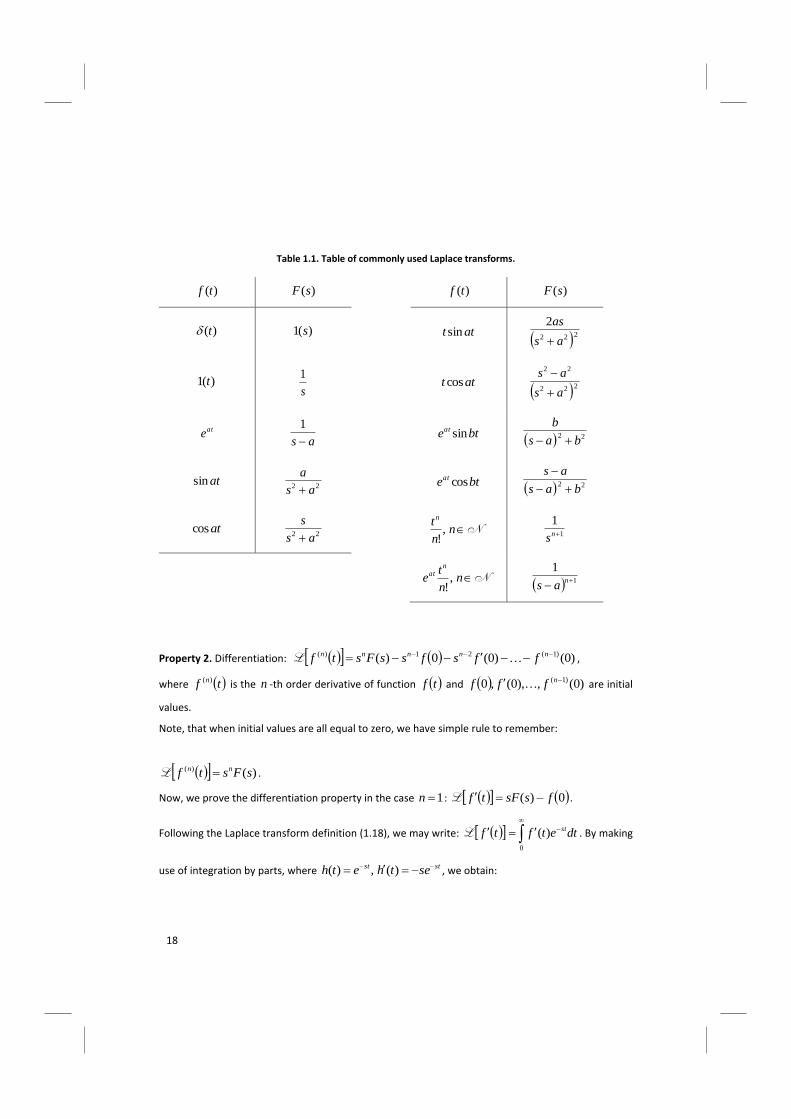
Table 1.1. Table of commonly used Laplace transforms.
)(tf )(sF )(tf )(sF
)(t )(1 s att sin 222
2
as
as
)(1 t s
1 attcos
222
22
as
as
ate as
1 bteat sin 22
bas
b
atsin 22 as
a
bteat cos 22
bas
as
atcos 22 as
s
Nn
n
tn
,!
1
1ns
Nnn
te
nat ,
!
1
1
n
as
Property 2. Differentiation: )0()0(0)( )1(21)( nnnnn ffsfssFstf L ,
where tf n)( is the n -th order derivative of function tf and )0(,),0(,0 )1( nfff are initial
values.
Note, that when initial values are all equal to zero, we have simple rule to remember:
)()( sFstf nn L .
Now, we prove the differentiation property in the case 1n : 0)( fssFtf L .
Following the Laplace transform definition (1.18), we may write:
0
)( dtetftf stL . By making
use of integration by parts, where stst setheth )(,)( , we obtain:
19
00
0
0
0
)()()()()()()( dtsetfetfdtthtfthtfdtetf ststst .
Assuming 0Re s gives: )0()()()0()(0
0 fssFdtetfsefetf stss
.
Property 3. Integration: )(1
sFs
df
t
o
L .
Recall, that in SIMULINK the integration block is labeled by s
1.
Property 4. Multiplication of a function by t : )(sFds
dttf L .
Now, we present short proof of the property above:
ttfdtettfdttftedttfeds
ddtetf
ds
dtf
ds
d stststst LL
0000
)()()()( .
Property 5. Division of a function by t :
s
dssFt
tf)(L .
Now, we present short proof of the property above:
.)()(
10)(
1)()()(
0
0000
t
tfdte
t
tf
dtet
tfdtet
tfdtdsetfdsdtetfdstf
st
st
s
st
s
st
s
st
s
L
L
Property 6. Multiplication of a function by ate : asFtfeat L .
Property 7. Change of time scale:
a
sF
aatf
1L , where 0a .
Now, we prove the property above. Following the Laplace transform definition (1.18), we may write:
20
0
)( dteatfatf stL . Taking atx we obtain:
a
sF
adxexf
aa
xdexf
xa
s
a
xs 1
)(1
)(00
.
Property 8. Delay: )(1 0
00 sFettttfst
L .
Now, we prove the delay property. Following the Laplace transform definition (1.18), we may write:
0
0
0
0000 11t
stst dtettfdtettttfttttfL . Taking 0tt we obtain:
)()( 00000
000
)(sFetfedefedeefdtef
ststsstststs
L
.
Property 9. Convolution:
)()()()()()()()( 2121
0
2121 sFsFtftfdftftftf
t
LLLL ,
where )()( 21 tftf is convolution of functions )(1 tf and )(2 tf .
Now, we prove the convolution property. At the beginning note, that 0)(1)(1 ttf holds for
t , which was assumed while defining Laplace transform (1.18). Following the Laplace transform
definition (1.18), we may write:
0
21
0
21 )()(1)()()( dfttfdftf
t
. Then:
0 0
21
0
21
0
21 )()(1)()()(1)()()( dtdfttfedfttfdftf st
t
LL .
Substituting t and changing the order of integration gives:
).()()()()()(
)()()()()()()()(
2121
0
2
0
1
0
2
0
)(
1
0
2
0
21
0
21
sFsFtftfdefdef
dfdefdfdteftatfdftf
ss
sst
t
LL
L
Example 1.6 – Using table of Laplace transforms. Work out Laplace transform of function
42sin53)( 2 tetf t .
With use of linearity property no. 1 together with table 1, we write:
21
.4
4
10
2
314
4
25
2
13142sin5342sin53
22
22
sssssstete tt
LLLL
Let us consider linear system with zero initial conditions, where dynamic relation between input
)(tu and output )(ty is described by differential equation (1.12):
.)()()()(
)()()()(
011
1
1
011
1
1
tubdt
tdub
dt
tudb
dt
tudb
tyadt
tdya
dt
tyda
dt
tyd
v
v
vv
v
v
m
m
mm
m
(1.20)
To transform both sides of this equation:
)()()()()()()()( 01
)1(
1
)(
01
)1(
1
)( tubtubtubtubtyatyatyaty v
v
v
v
m
m
m
LL .
Applying linearity property yields:
.)()()()(
)()()()(
01
)1(
1
)(
01
)1(
1
)(
tubtubtubtub
tyatyatyaty
v
v
v
v
m
m
m
LLLL
LLLL
Applying differentiation property no. 2, with zero initial values assumed, gives:
).()()()()()()()( 01
1
101
1
1 sUbssUbsUsbsUsbsYassYasYsasYs v
v
v
v
m
m
m
Pulling )(sY and )(sU before the bracket gives:
.)()( 01
1
101
1
1 bsbsbsbsUasasassY v
v
v
v
m
m
m
The transfer function )(sK of linear system with zero initial conditions is the ratio between Laplace
transform of the system output and the system input:
1
0
0
01
1
1
01
1
1
)(
)()(
m
i
i
i
m
v
i
i
i
m
m
m
v
v
v
vdf
sas
sb
asasas
bsbsbsb
sU
sYsK
. (1.21)
Example 1.7 – Evaluation of transfer function from differential equation. A linear system is
described by differential equation:
tu
dt
tduty
dt
tdy
dt
tyd223
2
2
. (1.22)
Passing both sides by Laplace transform gives:
)(2)()(2)(3)(2 sUssUsYssYsYs .
Pulling )(sY and )(sU before the bracket gives:
22
2)(23)( 2 ssUsssY .
Rearranging above equation gives transfer function:
)(23
2
)(
)(2
sKss
s
sU
sY
. (1.23)
Note, that description (1.23) makes sense for the system (1.22) only for zero initial conditions.
Example 1.8 – Evaluation of differential equation from transfer function. A linear system is
described by following transfer function:
1
1)(
ssK . (1.24)
We ask about differential equation describing the system:
1
1
)(
)(
ssU
sY .
Cross multiplication gives:
)(1)( sUssY ,
which is
)()()( sUsYssY .
Now we may deduce original difference equation:
)()()(
tutydt
tdy . (1.25)
Let us take a closer look at solution (1.23) of example 1.7:
1
1
)1)(2(
2
23
2)(
2
sss
s
ss
ssK .
We observe that two different differential equations (1.22) and (1.25) have the same transfer
function. Transfer function loses some information about the system. Differential equation is more
accurate description, however, transfer function is more convenient. When dealing with complex
systems, that are composed of many input-output dynamic elements, it is easy to work out the
complex system model on the basis of its elements transfer functions.
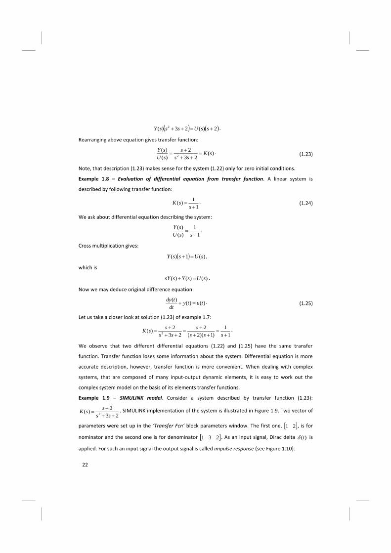
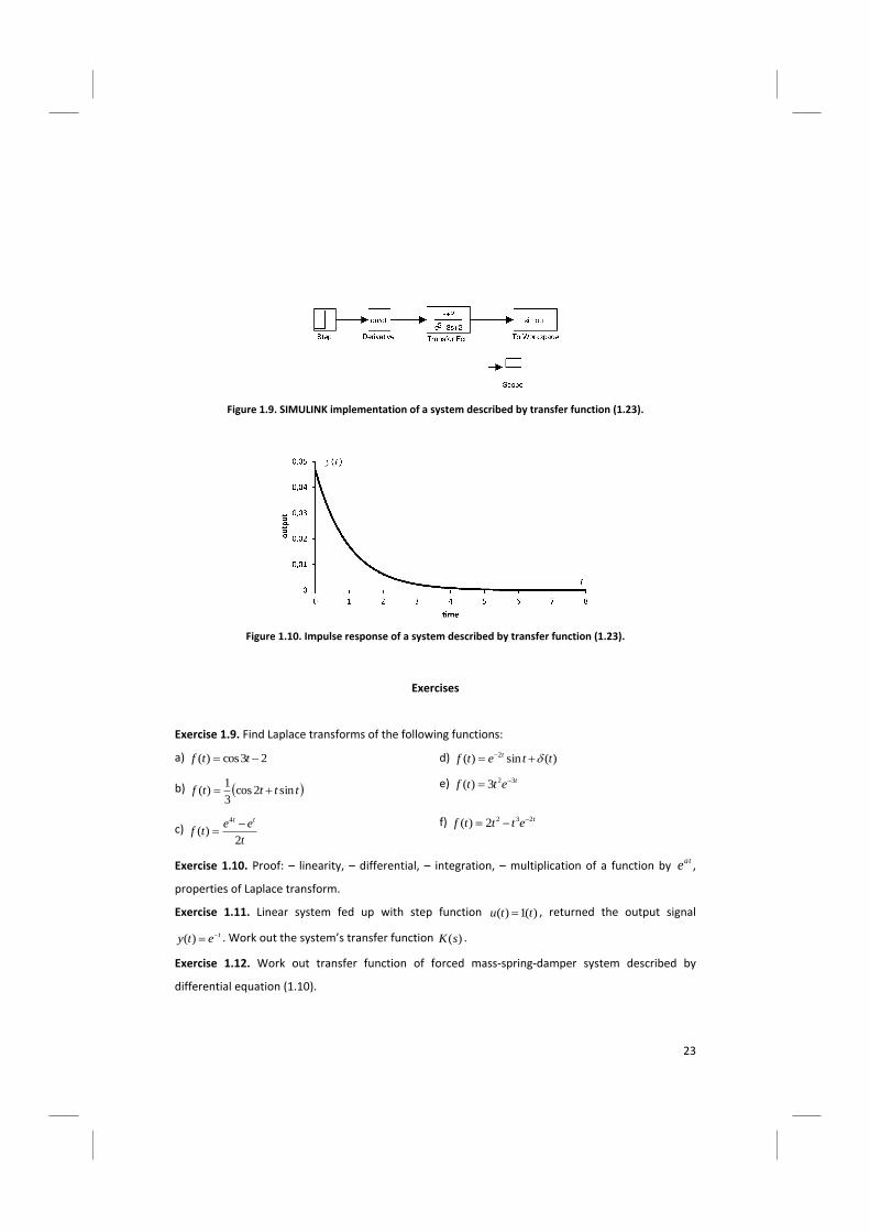
Example 1.9 – SIMULINK model. Consider a system described by transfer function (1.23):
23
2)(
2
ss
ssK . SIMULINK implementation of the system is illustrated in Figure 1.9. Two vector of
parameters were set up in the ‘Transfer Fcn’ block parameters window. The first one, 21 , is for
nominator and the second one is for denominator 231 . As an input signal, Dirac delta )(t is
applied. For such an input signal the output signal is called impulse response (see Figure 1.10).
23
Figure 1.9. SIMULINK implementation of a system described by transfer function (1.23).
Figure 1.10. Impulse response of a system described by transfer function (1.23).
Exercises
Exercise 1.9. Find Laplace transforms of the following functions:
a) 23cos)( ttf d) )(sin)( 2 ttetf t
b) ttttf sin2cos3
1)( e) tettf 323)(
c) t
eetf
tt
2)(
4
f) tetttf 2322)(
Exercise 1.10. Proof: – linearity, – differential, – integration, – multiplication of a function by ate ,
properties of Laplace transform.
Exercise 1.11. Linear system fed up with step function )(1)( ttu , returned the output signal
tety )( . Work out the system’s transfer function )(sK .
Exercise 1.12. Work out transfer function of forced mass-spring-damper system described by
differential equation (1.10).
24
Exercise 1.13. With use of SIMULINK implement models of systems described by transfer functions
(1.23), (1.24) and differential equations (1.22), (1.25). Compare their responses for different input
signals. What do you observe?
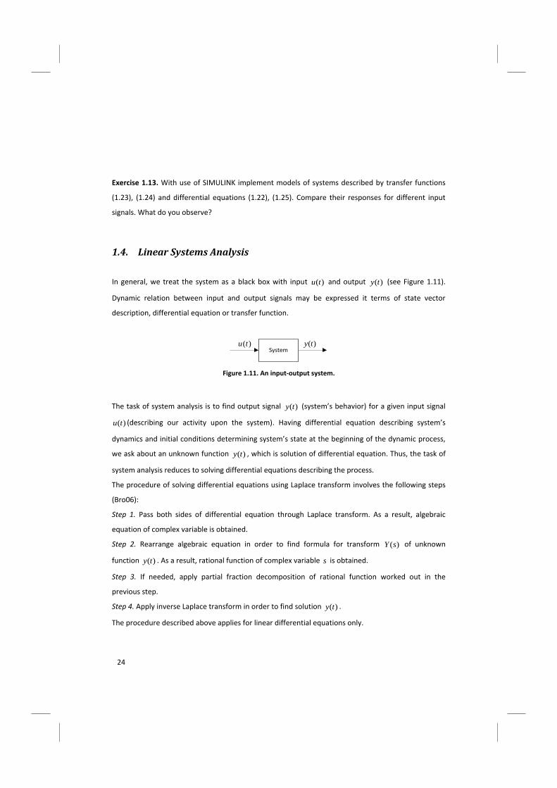
1.4. Linear Systems Analysis
In general, we treat the system as a black box with input )(tu and output )(ty (see Figure 1.11).
Dynamic relation between input and output signals may be expressed it terms of state vector
description, differential equation or transfer function.
System)(tu )(ty
Figure 1.11. An input-output system.
The task of system analysis is to find output signal )(ty (system’s behavior) for a given input signal
)(tu (describing our activity upon the system). Having differential equation describing system’s
dynamics and initial conditions determining system’s state at the beginning of the dynamic process,
we ask about an unknown function )(ty , which is solution of differential equation. Thus, the task of
system analysis reduces to solving differential equations describing the process.
The procedure of solving differential equations using Laplace transform involves the following steps
(Bro06):
Step 1. Pass both sides of differential equation through Laplace transform. As a result, algebraic
equation of complex variable is obtained.
Step 2. Rearrange algebraic equation in order to find formula for transform )(sY of unknown
function )(ty . As a result, rational function of complex variable s is obtained.
Step 3. If needed, apply partial fraction decomposition of rational function worked out in the
previous step.
Step 4. Apply inverse Laplace transform in order to find solution )(ty .
The procedure described above applies for linear differential equations only.
25
Example 1.10 – Solving linear differential equation.
Let us consider an input-output system described by following differential equation:
)()()(
2
2
tutydt
tyd .
Let us analyze the systems’ behavior activated by input signal ttu 2cos)( from zero initial
conditions: 0)0(
)0( dt
dyy . What does the output signal )(ty look like?
The problem reduces to solving unknown function )(ty from differential equation:
ttydt
tyd2cos)(
)(2
2
. (1.26)
At first, we pass both sides of the equation above by Laplace transform:
ttydt
tyd2cos)(
)(2
2
LL
.
Applying linearity property yields:
ttydt
tyd2cos)(
)(2
2
LLL
.
Using differentiation property for the left side and Laplace transform table for the right side gives
algebraic equation:
22
2
2)(
)0()0()(
s
ssY
dt
dysysYs .
Since all initial conditions are zero, we have:
22
2
2)()(
s
ssYsYs .
Taking )(sY before the bracket gives:
4
1)(2
2
s
sssY .
We obtain rational function:
)1)(4()(
22
ss
ssY ,
which partial fraction decomposition has the following form:
14)1)(4()(
2222
s
DCs
s
BAs
ss
ssY , (1.27)
26
where DCBA ,,, are coefficients to be determined in such a way, that equation above holds true. To
determine values of these coefficients, let us multiple both sides by denominator )1)(4( 22 ss :
41 22 sDCssBAss .
Brackets multiplication gives:
DDsCsCsBBsAsAss 44 2323 .
After elements of the same order are joined:
DBsCAsDBsCAs 4423 .
The equation above holds still if and only if the system of equations:
)d(04
)c(14
)b(0
)a(0
DB
CA
DB
CA
holds true. By subtraction of equation )a( from )c( and equation )b( from )d( :
)b()d(03
)a()c(13
D
C
we find that 0D and 31C . Then, from )b( we find that 0B and from )a( we have
31A . Going back to expression (1.27), we may write its form after partial fraction
decomposition:
13
1
43
1
)1)(4()(
2222
s
s
s
s
ss
ssY .
Now, it is easy to apply inverse Laplace transform:
13
1
23
1
13
1
43
1)()(
2
1
22
1
22
11
s
s
s
s
s
s
s
ssYty LLLL .
Eventually, using Laplace transforms table backwards, we obtain solution of differential equation
(1.26):
ttty cos3
12cos
3
1)( . (1.28)
As a result of analysis we found that considered system, driven by the signal ttu 2cos)( from the
zero state, responds with the signal ttty cos312cos31)( .
27
Exercises
Exercise 1.14. Work out numerical solution of differential equation (1.26) and compare it with the
exact one (1.28).
Exercise 1.15. Solve following differential equations:
a) ttydt
tydsin)(4
)(2
2
,
zero initial conditions
g) tetydt
tdy
dt
tyd
dt
tyd 6)()(
3)(
3)(
2
2
3
3
zero initial conditions
b) tdt
tyd
dt
tydcos
)()(3
3
4
4
,
zero initial conditions
h) ttydt
tdy
dt
tydsin
2
1)(14
)(9
)(2
2
,
1)0(
,0)0( dt
dyy
c) 2)()(
2 2 ttydt
tdy ,
4)0( y
i) tetydt
tdy
dt
tyd 3
2
2
4)(2)(
3)(
,
6)0(
,2)0( dt
dyy
d) tttydt
tyd3cos10sin3)(4
)(2
2
,
3)0(
,2)0( dt
dyy
j) tettydt
tdy
dt
tyd
dt
tyd 2
2
2
3
3
)()(
3)(
3)(
,
3)0(
,2)0(
,1)0(2
2
dt
yd
dt
dyy
e) tetydt
tdy
dt
tyd 2
2
2
3)(5)(
2)( ,
1)0(
,1)0( dt
dyy
k) 33)()( 2
2
2
ttetydt
tyd t ,
1)0(
,1)0( dt
dyy
f) )()(
3)(4)()(
2
2
tudt
tduty
dt
tdy
dt
tyd
zero initial conditions
Exercise 1.16. Try to solve differential equation 3
3
2
2 )()(
)(
dt
tudty
dt
tyd for zero initial conditions. Use
analytical method and numerical (in SIMULINK). Do you find anything wrong about this equation?
Exercise 1.17. Work out step response )(1)( ttu of linear system described by the transfer function
1
1)(
ssK .
28
Exercise 1.18. Work out impulse and step responses of a system described by differential equation:
)()()(
2)(
2
2
tutydt
tdy
dt
tyd .
1.5. Nonlinear Systems Analysis
Analysis of nonlinear systems is more challenging problem, due to limited possibilities of solving
nonlinear differential equations. There are some analytical methods, but for most nonlinear
equations that arise in practice only numerical solutions may be obtained. However, it is possible to
work out linear approximation of nonlinear system around a given state (usually called set point).
Usually set point is chosen as an equilibrium state of interest. Results of linearized system analysis
also apply for original nonlinear system in the neighborhood of a set point. For example, the stability
of nonlinear system may be stated on the basis of its linear approximation around a set point of
interest. Control algorithms may be designed for linearized systems and they should perform well as
long as the systems’ state stays close to the set point. If the systems goes far away from the chosen
set point , it should be linearized once again for different set point.
One of the simplest linearization procedure (Vuk03), based on the Taylor’s expansion, is given below.
Let us consider nonlinear system with the state vector description:
)(),()(
)(),()(
ttGt
ttFdt
td
uxy
uxx
. (1.29)
Nonlinear functions GF , are vector functions of the form:
)(),(
)(),(
)(),(
,,
)(),(
)(),(
)(),(
)(),(2
1
2
1
ttg
ttg
ttg
G
ttf
ttf
ttf
ttF
RR ux
ux
ux
ux
ux
ux
ux
ux
.
Let us denote a set point of interest by:
)(
)1(
)(
)1(
S
R
u
u
x
x
u
x .
29
Linear approximation of the system (1.29) has the general form:
)()()(
)()()(
ttt
ttdt
td
DuCxy
BuAxx
, (1.30)
where DCBA ,,, are matrices containing constant number determined using the following
definitions:
uuxx
uuxxx
A
)()1(
)(
1
)1(
1
R
RR
R
x
f
x
f
x
f
x
f
F
, (1.31)
uuxx
uuxxu
B
)()1(
)(
1
)1(
1
S
RR
S
u
f
u
f
u
f
u
f
F
, (1.32)
uuxx
uuxxx
C
)()1(
)(
1
)1(
1
R
LL
R
x
g
x
g
x
g
x
g
G
, (1.33)
uuxx
uuxxu
D
)()1(
)(
1
)1(
1
S
LL
S
u
g
u
g
u
g
u
g
G
. (1.34)
Example 1.11 – Linearization of state vector description.
Let us take a system described by the following state vector description:
)()()(
)(2)(sin)(2)(
)()()()()(3)(
)1(
)1()()1()2(
22)2()2()1()2()1(
)2(
tutxty
tutxetxdt
tdx
tutxtxtxtxdt
tdx
tx (1.35)
State vector for the system above has two dimensions:
,)(
)()(
)2(
)1(
tx
txtx , and )()( tut u .
30
Functions GF , also have two dimensions:
)(),()(),(,)(),(
)(),()(),(
2
1ttgttG
ttf
ttfttF uxux
ux
uxux
,
where functions gff ,, 21 are:
)()()(),(
)(2)(sin)(2)(),(
)()()()()(3)(),(
)1(
)1()()1(
2
22)2()2()1()2(
1
)2(
tutxttg
tutxetxttf
tutxtxtxtxttf
tx
ux
ux
ux
.
Matrices introduced in (1.30) have the form given by (1.31)-(1.34):
uuxx
uuxx
uuxx
uuxx
DCBA
u
g
x
g
x
g
u
f
u
f
x
f
x
f
x
f
x
f
,,,)2()1(
2
1
)2(
2
)1(
2
)2(
1
)1(
1
. (1.36)
Components of these matrices are evaluated as:
)()2(
)1(
1 tuxx
f
, )(2)(3 )2()1(
)2(
1 txtxx
f
,
)(cos2 )1()(
)1(
2)2(
txex
f tx
, )(sin )1()(
)2(
2)2(
txex
f tx
,
)(21 tuu
f
, 22
u
f,
1)1(
x
g, 0
)2(
x
g, 1
u
g.
Introducing the formulas above to (1.36), we obtain description of linearized systems:
)()(01)(
)(2
)(2)(
)(sin)(cos2
)(2)(3)()()1()()1()(
)2()1()2(
)2()2(
ttt
ttu
ttxetxe
txtxtx
dt
tdtxtx
uxy
uxx
uuxx
uuxx . (1.37)
As an example, we chose the set point as the zero vector:
0
0
0)2(
)1(
u
x
x
.
31
For this particular point the system (1.37) has the form:
)()(01)(
)(2
0)(
01
30)(
ttt
ttdt
td
uxy
uxx
.
Exercises
Exercise 1.19. Linearize the system below:
2)2()1(
)1()1()2(
2)2(2)1(
)2()1(
1)()()()(
)(1)()(
)(sin)()()(1
)()(
tutxtxty
txtuxdt
tdx
tututxtx
tx
dt
tdx
around the zero set point:
0
0
0)2(
)1(
u
x
x
.
Exercise 1.20.
Linearize the state vector description of inverted pendulum, obtained when solving exercise 1.8
around the unstable equilibrium position (zero angle of displacement and zero angular velocity).
When the system is more sensitive to control actions and disturbances: for long or for short
pendulum?
32
2. Identification
Identification is the term describing mathematical tools and algorithms to build models of real
systems from measured data. These models are significant in many disciplines. They can be used to
formulate both new research and engineering problems. The models are useful for system analysis,
to get better understanding of the real systems (Bub80, Nel01).
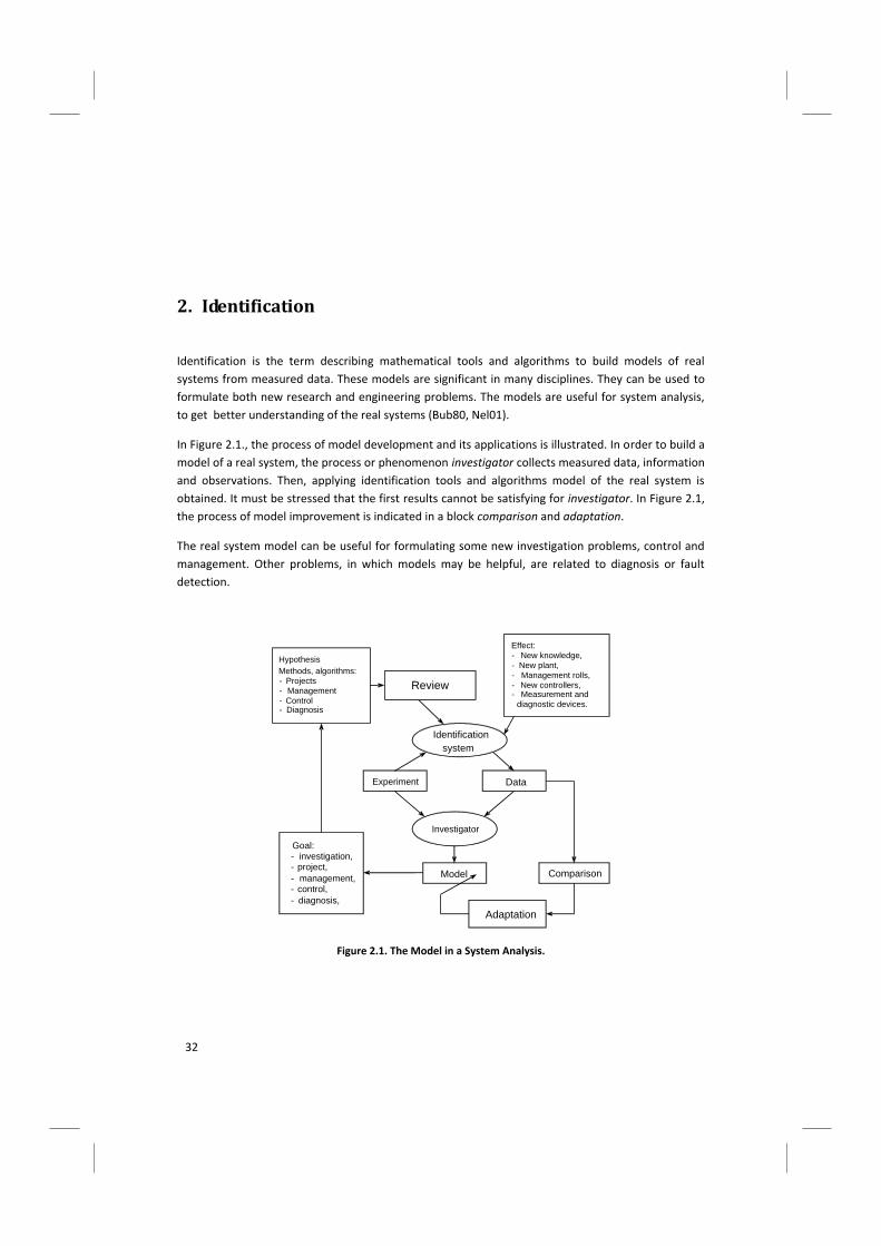
In Figure 2.1., the process of model development and its applications is illustrated. In order to build a
model of a real system, the process or phenomenon investigator collects measured data, information
and observations. Then, applying identification tools and algorithms model of the real system is
obtained. It must be stressed that the first results cannot be satisfying for investigator. In Figure 2.1,
the process of model improvement is indicated in a block comparison and adaptation.
The real system model can be useful for formulating some new investigation problems, control and
management. Other problems, in which models may be helpful, are related to diagnosis or fault
detection.
Hypothesis
Methods, algorithms:
- Projects
- Management
- Control- Diagnosis
Review
Effect:
- New knowledge,
- New plant,
- Management rolls,
- New controllers,- Measurement and
diagnostic devices.
Identification
system
Experiment Data
Investigator
Model Comparison
Adaptation
Goal:- investigation,- project,
- management,- control,
- diagnosis,
Figure 2.1. The Model in a System Analysis.
33
As the result of findings mentioned above problems, we have obtained some hypothesis and
methods for new control, management and diagnosis algorithms. After verification of acquired
outcomes, we have some new knowledge on investigated real systems. Developed control and
management algorithms are applied in a design process of new controllers and management systems
(Figure 2.1).
2.1 Determination of the System Parameters
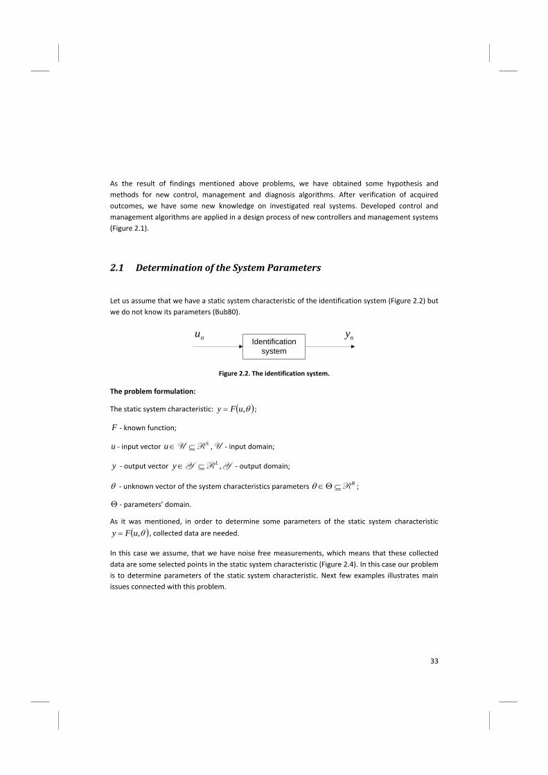
Let us assume that we have a static system characteristic of the identification system (Figure 2.2) but
we do not know its parameters (Bub80).
Identification
system
nu ny
Figure 2.2. The identification system.
The problem formulation:
The static system characteristic: ,uFy ;
F - known function;
u - input vector Su RU ,U - input domain;
y - output vector Ly RY ,Y - output domain;
- unknown vector of the system characteristics parameters RR ;
- parameters’ domain.
As it was mentioned, in order to determine some parameters of the static system characteristic
,uFy , collected data are needed.
In this case we assume, that we have noise free measurements, which means that these collected
data are some selected points in the static system characteristic (Figure 2.4). In this case our problem
is to determine parameters of the static system characteristic. Next few examples illustrates main
issues connected with this problem.
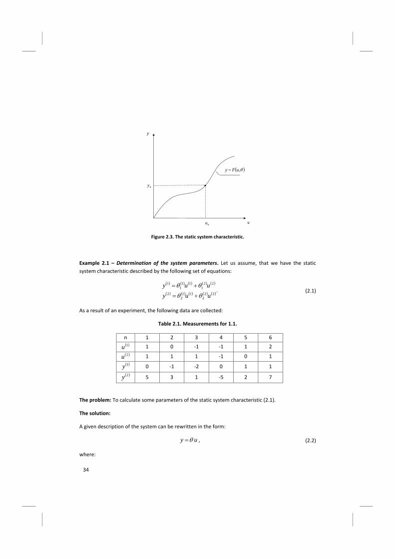
34
y
ny
u
,uFy
nu
Figure 2.3. The static system characteristic.
Example 2.1 – Determination of the system parameters. Let us assume, that we have the static
system characteristic described by the following set of equations:
22
2
11
2
2
22
1
11
1
1
uuy
uuy
. (2.1)
As a result of an experiment, the following data are collected:
Table 2.1. Measurements for 1.1.
n 1 2 3 4 5 6 1u 1 0 -1 -1 1 2
2u 1 1 1 -1 0 1
1y 0 -1 -2 0 1 1
2y 5 3 1 -5 2 7
The problem: To calculate some parameters of the static system characteristic (2.1).
The solution:
A given description of the system can be rewritten in the form:
uy , (2.2)
where:
35
2
1
u
uu ,
2
1
y
yy ,
2
2
1
2
2
1
1
1
. (2.3)
In the first step we have to decide, how many measurements are needed to solve the given
problem. As we know, to calculate unknown parameters of the static system characteristic (2.1),
following condition must be fulfilled:
RLN , (2.4)
where:
N - number of measurements;
L - dimensionality of the output vector;
R - dimensionality of unknown vector of parameters for the static system characteristic.
Because, in our example, 2L , 4R , it means that the minimal number of measurements, which
are needed to solve the problem, is 2N .
In the next step we have to select N = 2 measurements from the table 2.1, which fulfills identification
conditions. It means that for matrix of input measurements NU we must obtain:
0det NU . (2.5)
Let us choose from table 2.1 measurement 1n and 4n . Matrix NU has form:
11
11NU . (2.6)
The identification condition can be verified in the following way:
011
11det
NU . (2.7)
The obtained result means that for selected measurements ( 1n and 4n ) it is not possible to
find the solution: a proposed sequence does not form identifiable sequence.
Let us try with a new set of measurements: 2n and 5n . Determinant of NU is as follows:
101
10det
NU . (2.8)
Because 0det NU means that we have found identifiable sequence, it can possible determine a
set of parameters of static system’s characteristic (2.1).
In the next step we have to determine identification algorithm, to calculate unknown parameters of a
given characteristic (2.1).
36
Let us rewrite an equation (2.2), taking into account that 2N :
22 UY , (2.9)
where:
212 yyY , 212 uuU , (2.10)
and
1
2
1
2
21
1
1
1
1 ,y
yy
y
yy ,
1
2
1
2
21
1
1
1
1 ,u
uu
u
uu . (2.11)
In order to determine , we have to solve the matrix equation (2.9): 1
22
1
22
UUUY . (2.12)
Finally, the algorithm to determine vector of parameters has the form: 1
22
UY . (2.13)
Now, we can substitute in (2.13) measurements 2n and 5n . As the result, the following matrix
equations are obtained: 1
01
10
23
11
, (2.14)
and then we can get this solution:
32
11
01
10
23
11
01
10
23
111
. (2.15)
Verification of the solution:
Let us choose 1n and 6n . We can verify obtained results substituting in matrix 2U (2.9) data
1n , 6n and check that the determined values of the output are the same, as in the table 2.1:
75
10
11
21
32
112Y . (2.16)
It is easy to notice that the same results will be obtained for other measurements set, providing that
they form identifiable sequence.
Example 2.2 – Determination of the system’s parameter. Let us assume that we have some static
system characteristic described by following equation:
2321 uuy . (2.17)
37
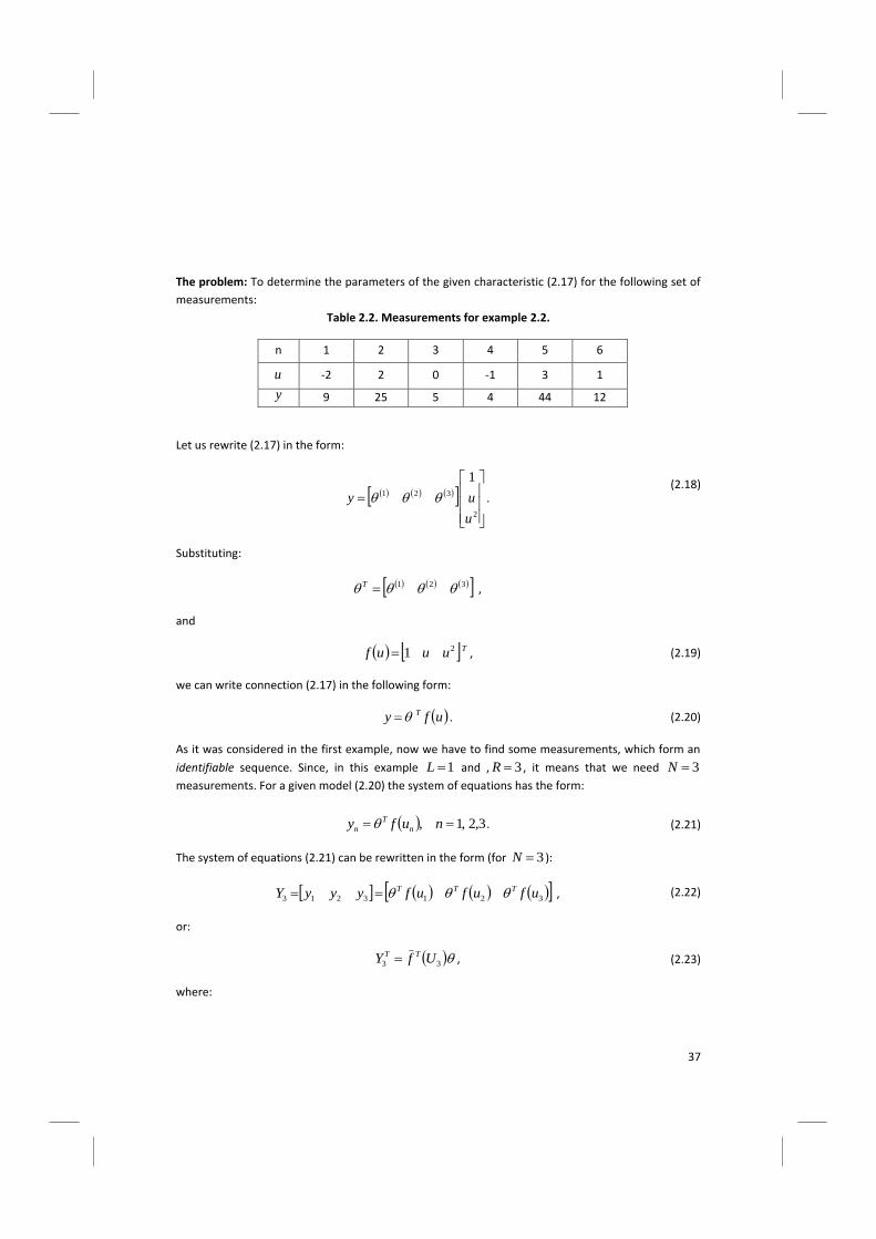
The problem: To determine the parameters of the given characteristic (2.17) for the following set of
measurements:
Table 2.2. Measurements for example 2.2.
n 1 2 3 4 5 6
u -2 2 0 -1 3 1
y 9 25 5 4 44 12
Let us rewrite (2.17) in the form:
2
321
1
u
uy .
(2.18)
Substituting:
321 T ,
and
Tuuuf 21 ,
(2.19)
we can write connection (2.17) in the following form:
ufy T .
(2.20)
As it was considered in the first example, now we have to find some measurements, which form an
identifiable sequence. Since, in this example 1L and , 3R , it means that we need 3N
measurements. For a given model (2.20) the system of equations has the form:
3,2,1, nufy n
T
n . (2.21)
The system of equations (2.21) can be rewritten in the form (for 3N ):
3213213 ufufufyyyY TTT , (2.22)
or:
33 UfY TT , (2.23)
where:
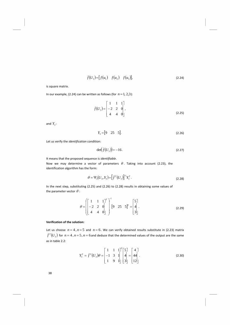
38
3213 ufufufUf , (2.24)
is square matrix.
In our example, (2.24) can be written as follows (for 3,2,1n ):
044
022
111
3Uf ,
(2.25)
and 3Y :
52593 Y . (2.26)
Let us verify the identification condition:
16det 3 Uf . (2.27)
It means that the proposed sequence is identifiable.
Now we may determine a vector of parameters . Taking into account (2.23), the
identification algorithm has the form:
TT YUfYU 3
1
3333 ,
.
(2.28)
In the next step, substituting (2.25) and (2.26) to (2.28) results in obtaining some values of
the parameter vector :
3
4
5
5259
044
022
1111
T
T
.
(2.29)
Verification of the solution:
Let us choose 4n , 5n and 6n . We can verify obtained results substitute in (2.23) matrix
3Uf T for 4n , 5n , 6n and deduce that the determined values of the output are the same
as in table 2.2:
12
44
4
3
4
5
191
131
111
33
T
TT UfY . (2.30)
39
It is easy to notice that the same results will be obtained for other measurements set, provided that
they form the identifiable sequence.
Exercises
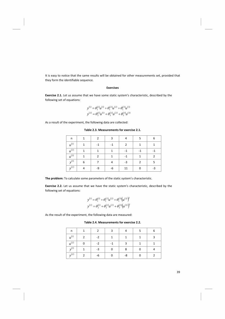
Exercise 2.1. Let us assume that we have some static system’s characteristic, described by the
following set of equations:
33
2
22
2
11
2
2
33
1
22
1
11
1
1
uuuy
uuuy
As a result of the experiment, the following data are collected:
Table 2.3. Measurements for exercise 2.1.
n 1 2 3 4 5 6
1u 1 -1 -1 2 1 1
2u 1 1 1 -1 -1 -1
3u 1 2 1 -1 1 2
1y 6 7 4 -3 2 5
2y 4 -9 -6 11 0 -3
The problem: To calculate some parameters of the static system’s characteristic.
Exercise 2.2. Let us assume that we have the static system’s characteristic, described by the
following set of equations:
233
2
22
2
1
2
2
233
1
22
1
1
1
1
uuy
uuy
As the result of the experiment, the following data are measured:
Table 2.4. Measurements for exercise 2.2.
n 1 2 3 4 5 6
1u 2 -2 1 1 1 3
2u 0 -2 -1 3 1 1
1y 1 -3 0 8 0 4
2y 2 -6 0 -8 0 2
40
The problem: To calculate some parameters of the static system’s characteristic.
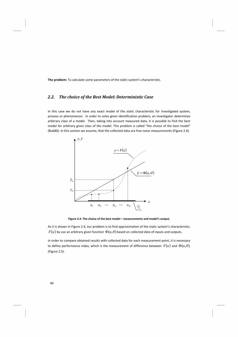
2.2. The choice of the Best Model: Deterministic Case
In this case we do not have any exact model of the static characteristic for investigated system,
process or phenomenon. In order to solve given identification problem, an investigator determines
arbitrary class of a model. Then, taking into account measured data, it is possible to find the best
model for arbitrary given class of the model. This problem is called “the choice of the best model”
(Bub80). In this section we assume, that the collected data are free noise measurements (Figure 2.4).
ny
u
yy,
uFy
ny
,uy
uD 1u 2u nu Nu … …
Figure 2.4. The choice of the best model – measurements and model’s output.
As it is shown in Figure 2.4, our problem is to find approximation of the static system’s characteristic,
uF by use an arbitrary given function ),( u based on collected data of inputs and outputs.
In order to compare obtained results with collected data for each measurement point, it is necessary
to define performance index, which is the measurement of difference between uF and ),( u
(Figure 2.5).
41
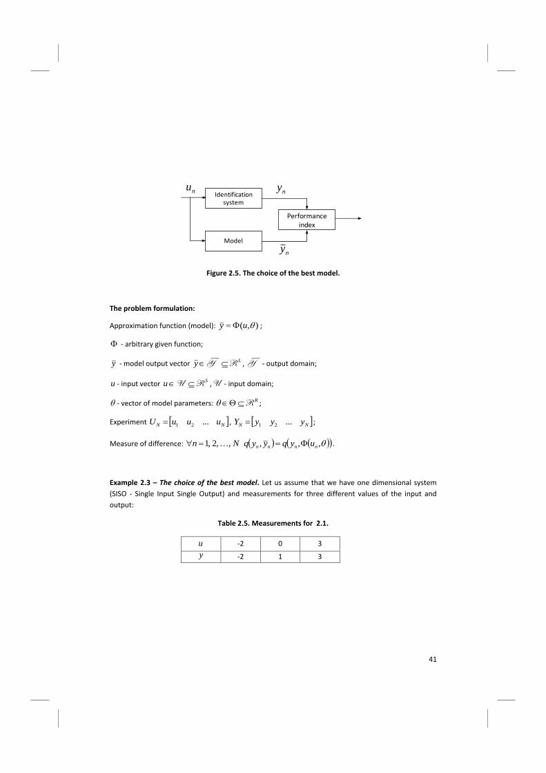
Identificationsystem
Model
Performance index
nynu
ny
Figure 2.5. The choice of the best model.
The problem formulation:
Approximation function (model): ),( uy ;
- arbitrary given function;
y - model output vector Ly RY , Y - output domain;
u - input vector Su RU ,U - input domain;
- vector of model parameters: RR ;
Experiment NN uuuU ...21 , NN yyyY ...21 ;
Measure of difference: Nn ,,2,1 ,,, nnnn uyqyyq .
Example 2.3 – The choice of the best model. Let us assume that we have one dimensional system
(SISO - Single Input Single Output) and measurements for three different values of the input and
output:
Table 2.5. Measurements for 2.1.
u -2 0 3
y -2 1 3
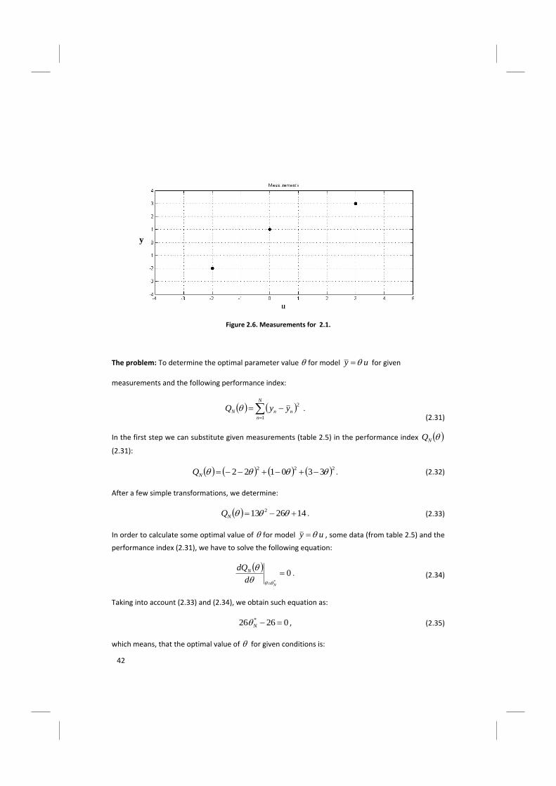
42
Figure 2.6. Measurements for 2.1.
The problem: To determine the optimal parameter value for model uy for given
measurements and the following performance index:
N
n
nnN yyQ1
2 .
(2.31)
In the first step we can substitute given measurements (table 2.5) in the performance index NQ
(2.31):
222330122 NQ . (2.32)
After a few simple transformations, we determine:
142613 2 NQ . (2.33)
In order to calculate some optimal value of for model uy , some data (from table 2.5) and the
performance index (2.31), we have to solve the following equation:
0
*
N
d
dQN
. (2.34)
Taking into account (2.33) and (2.34), we obtain such equation as:
02626 * N , (2.35)
which means, that the optimal value of for given conditions is:
y
43
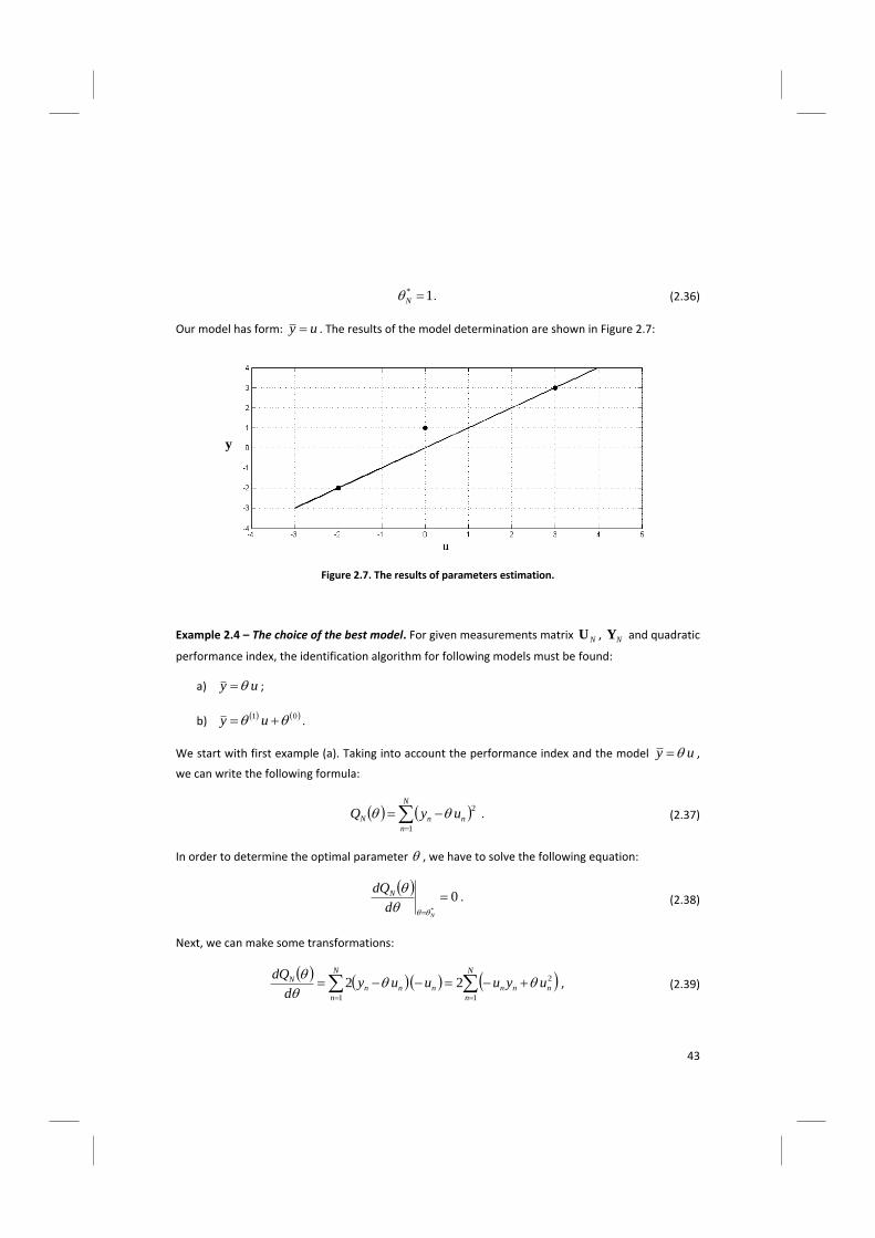
1* N . (2.36)
Our model has form: uy . The results of the model determination are shown in Figure 2.7:
Figure 2.7. The results of parameters estimation.
Example 2.4 – The choice of the best model. For given measurements matrix NU , NY and quadratic
performance index, the identification algorithm for following models must be found:
a) uy ;
b) 01 uy .
We start with first example (a). Taking into account the performance index and the model uy ,
we can write the following formula:
N
n
nnN uyQ1
2 . (2.37)
In order to determine the optimal parameter , we have to solve the following equation:
0
*
N
d
dQN
. (2.38)
Next, we can make some transformations:
N
n
nnnn
N
n
nnN uyuuuy
d
dQ
1
2
1
22
, (2.39)
y
44
and then
021
2*
N
n
nNnn uyu ,
(2.40)
01
2*
1
N
n
nN
N
n
nn uyu , (2.41)
N
n
nn
N
n
nN yuu11
2* . (2.42)
Finally, the algorithm to calculate the optimal value of parameter has a form:
N
n
n
N
n
nn
N
u
yu
1
2
1* . (2.43)
Let us now consider the same problem of calculating some optimal values of the parameters vector,
but for the second model (b) 01 uy . All conditions remain the same. The performance
index for this problem has the form:
N
n
nn
N
n
nnN uyuyQ1
201
1
201 . (2.44)
In this example the performance index depends on two variables i.e.: 0 and 1 . It means that we
have to solve the set of equations which fulfills the following condition:
20* N
Q . (2.45)
We can rewrite it as:
00*
0
N
Q
, (2.46)
01*
1
N
Q
. (2.47)
Taking into account equations (2.44) and (2.45), we can determine such derivatives for
variable 0 :
45
N
n
nn
N
n
nn uyuyQ
1
01
1
01
0212
, (2.48)
and 1 :
N
n
nnnn
N
n
nnn uuyuuuyQ
1
021
1
01
122
.
(2.49)
Now, we focus on the equation (2.48):
021
0*1*
N
n
NnNn uy ,
(2.50)
01
1*
1
0*
1
N
n
nN
N
n
N
N
n
n uy , (2.51)
011
1*
1
0*
1
N
n
nN
N
n
N
N
n
n uy , (2.52)
N
n
n
N
n
nNN yuN11
1*0* , (2.53)
N
n
n
N
n
nNN yN
uN 11
1*0* 11 , (2.54)
and (2.49):
021
0*21*
N
n
nNnNnn uuyu ,
(2.55)
01
21*
1
0*
1
N
n
nN
N
n
nN
N
n
nn uuyu ,
(2.56)
46
N
n
nn
N
n
nN
N
n
nN yuuu11
21*
1
0* . (2.57)
For sake of simplicity, let us substitute:
N
n
nuN
u1
1ˆ and
N
n
nyN
y1
1ˆ . Now, we can rewrite some
connections between (2.54) and (2.57) in the form:
yuNNˆˆ1*0* , (2.58)
N
n
nn
N
n
nNN yuN
uN
u11
21*0* 11ˆ .
(2.59)
From (2.58) we can determine:
uy NNˆˆ 1*0* . (2.60)
Substituting (2.60) in (2.59) we obtain:
N
n
nn
N
n
nNN yuN
uN
uuy11
21*1* 11ˆˆˆ ,
(2.61)
and then
N
n
nn
N
n
nNN yuN
uN
uuy11
21*21* 11ˆˆˆ .
(2.62)
We can rewrite (2.61) in the form:
N
n
nn
N
n
nN yuN
uyuuN 1
2
1
21* 1ˆˆˆ
1 ,
(2.63)
and finally:
2
1
2
11*
ˆ1
ˆˆ1
uuN
uyyuN
N
n
n
N
n
nn
N
.
(2.64)
Let us summarize our calculations determining the algorithm to estimate two-dimensional variable
, i.e.:
47
uy NNˆˆ 1*0* , (2.65)
2
1
2
10*
ˆ1
ˆˆ1
uuN
uyyuN
N
n
n
N
n
nn
N
.
(2.66)
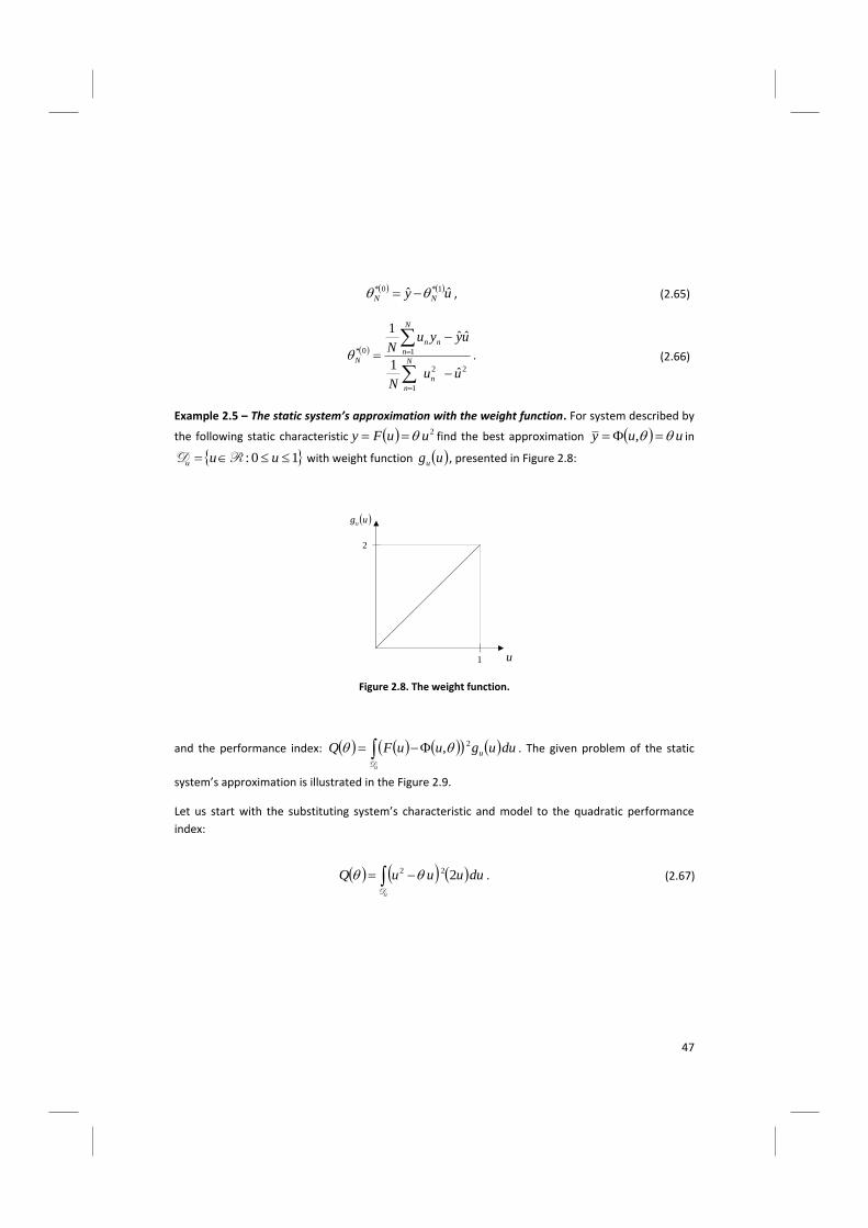
Example 2.5 – The static system’s approximation with the weight function. For system described by
the following static characteristic 2uuFy find the best approximation uuy , in
10: uuu RD with weight function ugu , presented in Figure 2.8:
ugu
u
2
1
Figure 2.8. The weight function.
and the performance index: duuguuFQ
u
u D
2, . The given problem of the static
system’s approximation is illustrated in the Figure 2.9.
Let us start with the substituting system’s characteristic and model to the quadratic performance
index:
u
duuuuQD
222 .
(2.67)
48
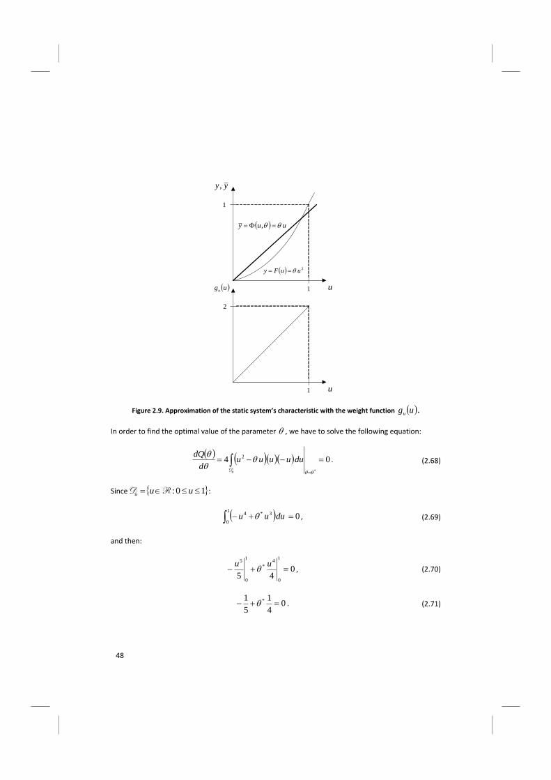
yy ,
u
1
1
2uuFy
uuy ,
ugu
u
2
1
Figure 2.9. Approximation of the static system’s characteristic with the weight function ugu .
In order to find the optimal value of the parameter , we have to solve the following equation:
04*
2
u
duuuuud
dQ
D
. (2.68)
Since 10: uuu RD :
01
0
3*4 duuu , (2.69)
and then:
045
1
0
4*
1
0
5
uu
, (2.70)
04
1
5
1 * . (2.71)
49
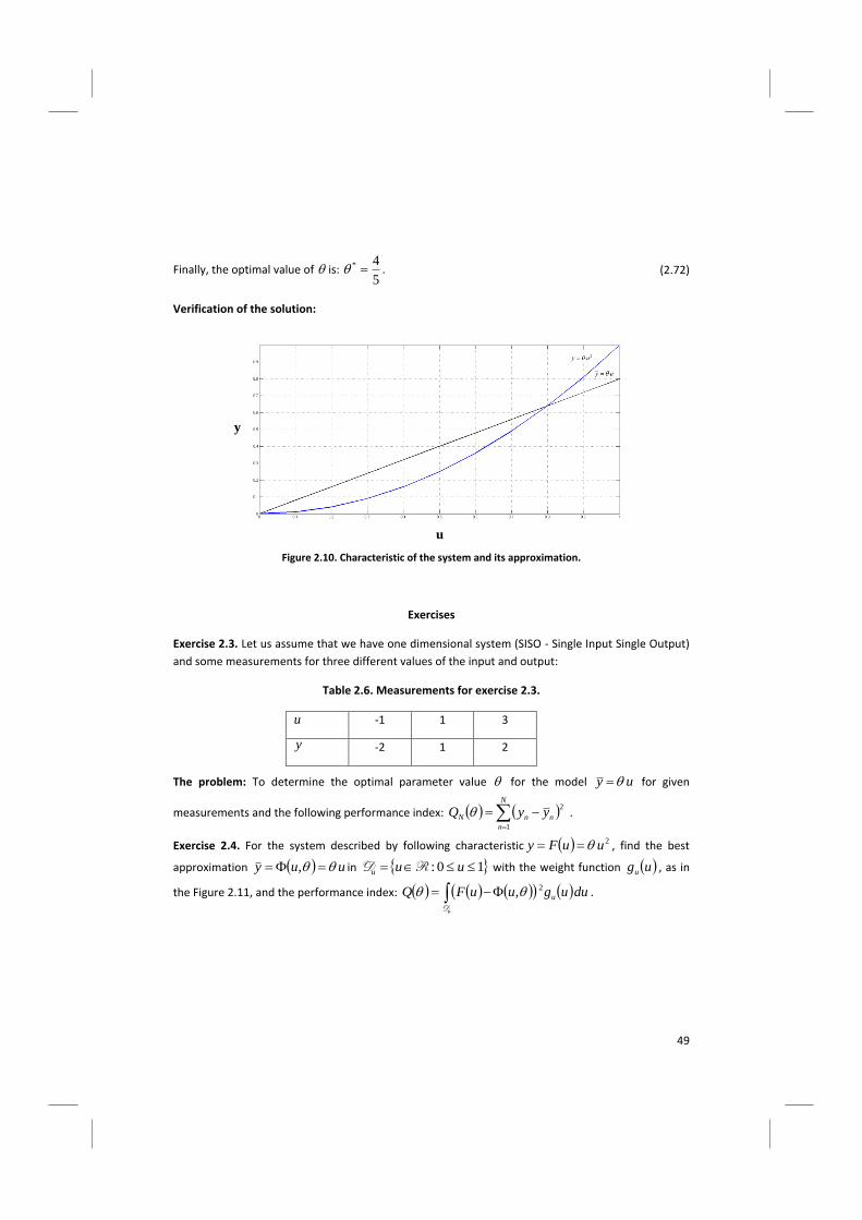
Finally, the optimal value of is: 5
4* . (2.72)
Verification of the solution:
Figure 2.10. Characteristic of the system and its approximation.
Exercises
Exercise 2.3. Let us assume that we have one dimensional system (SISO - Single Input Single Output)
and some measurements for three different values of the input and output:
Table 2.6. Measurements for exercise 2.3.
u -1 1 3
y -2 1 2
The problem: To determine the optimal parameter value for the model uy for given
measurements and the following performance index:
N
n
nnN yyQ1
2 .
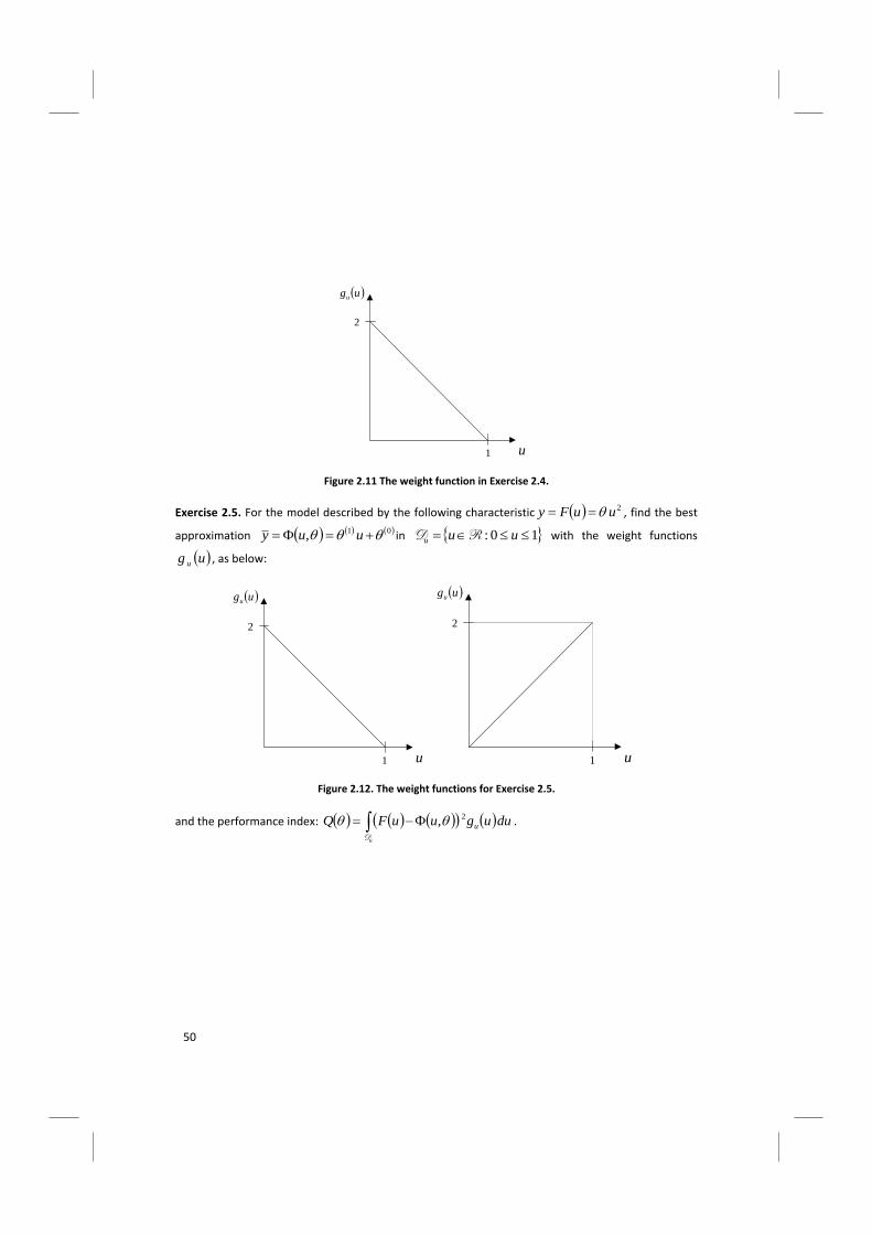
Exercise 2.4. For the system described by following characteristic 2uuFy , find the best
approximation uuy , in 10: uuu RD with the weight function ugu , as in
the Figure 2.11, and the performance index: duuguuFQ
u
u D
2, .
y
u
50
ugu
u
2
1
Figure 2.11 The weight function in Exercise 2.4.
Exercise 2.5. For the model described by the following characteristic 2uuFy , find the best
approximation 01, uuy in 10: uuu RD with the weight functions
ug u , as below:
ugu
u
2
1
ugu
u
2
1
Figure 2.12. The weight functions for Exercise 2.5.
and the performance index: duuguuFQ
u
u D
2, .
51
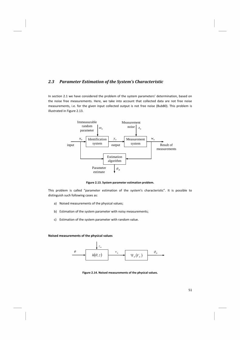
2.3 Parameter Estimation of the System’s Characteristic
In section 2.1 we have considered the problem of the system parameters’ determination, based on
the noise free measurements. Here, we take into account that collected data are not free noise
measurements, i.e. for the given input collected output is not free noise (Bub80). This problem is
illustrated in Figure 2.13.
Immeasurable random
parameter
input
output
Measurement
noise
Result of
measurements
Parameter
estimate
Identification
system
nu ny Measurement
system
nz
nw
Estimation
algorithm
N
n
Figure 2.13. System parameter estimation problem.
This problem is called “parameter estimation of the system’s characteristic”. It is possible to
distinguish such following cases as:
a) Noised measurements of the physical values;
b) Estimation of the system parameter with noisy measurements;
c) Estimation of the system parameter with random value.
Noised measurements of the physical values
Figure 2.14. Noised measurements of the physical values.
52
The problem formulation:
Measurement noise:
nz – value of random variable z from space Z ;
zf z – probability density function;
– observed vector of parameters, value of random variable , RR ;
f – probability density function;
Measurements: NN vvvV 21 .
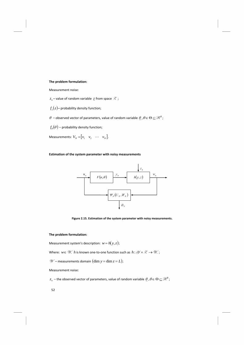
Estimation of the system parameter with noisy measurements
Figure 2.15. Estimation of the system parameter with noisy measurements.
The problem formulation:
Measurement system’s description: zyhw , ;
Where: W,w h is known one-to-one function such as W,ZY :h ;
W – measurements domain Lzy dimdim ;
Measurement noise:
nz – the observed vector of parameters, value of random variable , RR ;
53
f – value of random variable f from space Z ;
zf z – probability density function;
Measurements: NNNN wwwWuuuU 2121 , .
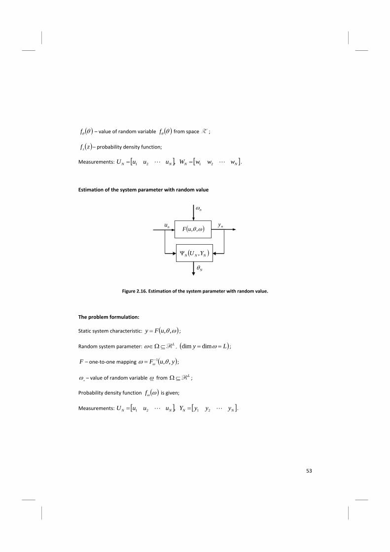
Estimation of the system parameter with random value
N
,,uF nu
n
ny
NNN YU ,
Figure 2.16. Estimation of the system parameter with random value.
The problem formulation:
Static system characteristic: ,,uFy ;
Random system parameter: LyL dimdim,R ;
F – one-to-one mapping yuF ,,1 ;
n – value of random variable from LR ;
Probability density function f is given;
Measurements: NNNN yyyYuuuU 2121 , .
54
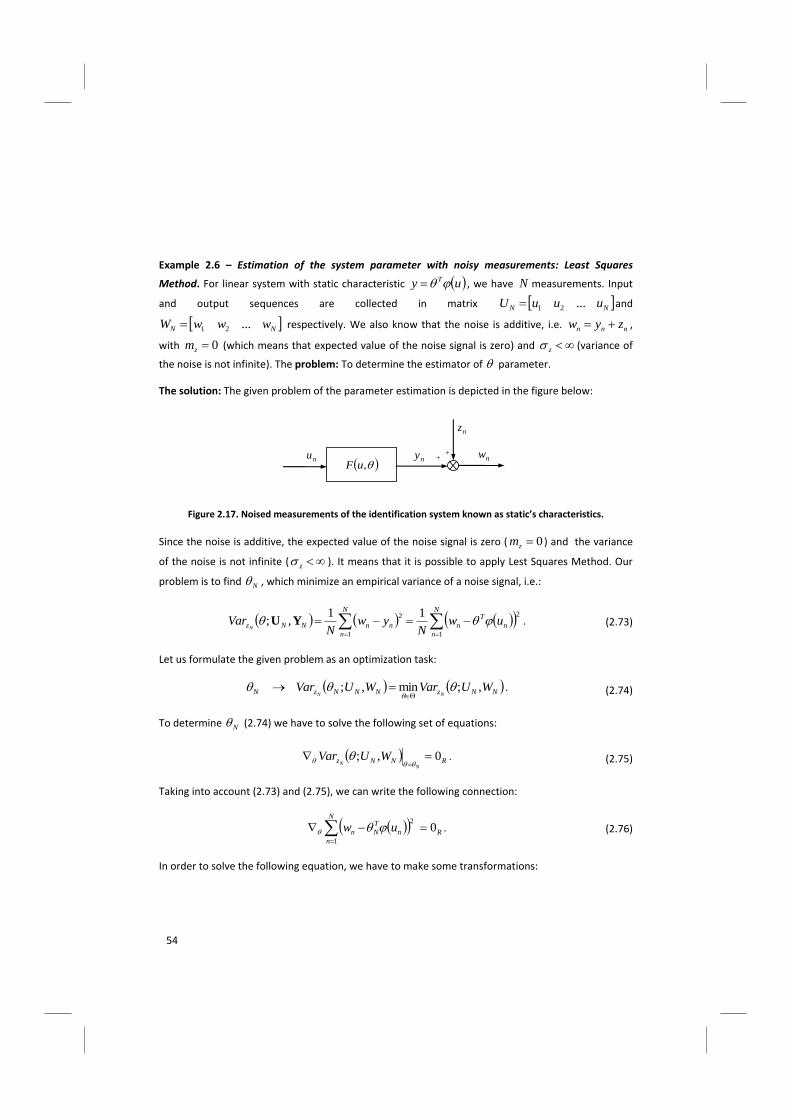
Example 2.6 – Estimation of the system parameter with noisy measurements: Least Squares
Method. For linear system with static characteristic uy T , we have N measurements. Input
and output sequences are collected in matrix NN uuuU ...21 and
NN wwwW ...21 respectively. We also know that the noise is additive, i.e. nnn zyw ,
with 0zm (which means that expected value of the noise signal is zero) and z (variance of
the noise is not infinite). The problem: To determine the estimator of parameter.
The solution: The given problem of the parameter estimation is depicted in the figure below:
,uF
nu ny
nz
nw
Figure 2.17. Noised measurements of the identification system known as static’s characteristics.
Since the noise is additive, the expected value of the noise signal is zero ( 0zm ) and the variance
of the noise is not infinite ( z ). It means that it is possible to apply Lest Squares Method. Our
problem is to find N , which minimize an empirical variance of a noise signal, i.e.:
N
n
n
T
n
N
n
nnNNz uwN
ywN
VarN
1
2
1
2 11,; YU . (2.73)
Let us formulate the given problem as an optimization task:
NNzNNNzN WUVarWUVarNN
,;min,;
. (2.74)
To determine N (2.74) we have to solve the following set of equations:
RNNzN
NWUVar 0,;
. (2.75)
Taking into account (2.73) and (2.75), we can write the following connection:
R
N
n
n
T
Nn uw 01
2
. (2.76)
In order to solve the following equation, we have to make some transformations:
55
R
N
n
nn
T
Nn uuw 021
, (2.77)
we can simplify our connection:
R
N
n
T
n
T
Nn
N
n
nn uuuw 011
, (2.78)
R
N
n
N
T
nn
N
n
nn uuuw 011
, (2.79)
R
N
n
N
T
nn
N
n
nn uuuw 011
. (2.80)
Finally, an algorithm to determine N has form:
N
n
nn
N
n
T
nnN uwuu1
1
1
. (2.81)
Example 2.7 – Estimation of the system parameter with noisy measurements: Maximum Likelihood
Method. For fixed sequence of inputs Nuuu ,...,, 21 and for linear system with characteristic uy ,
it was collected following sequence of noised outputs Nwww ,...,, 21 . The problem: to determine the
estimator of parameter for the additive noise ( nnn zyw ) and probability density function
2
2
2exp
2
1
z
zz
mzzf
.
The solution: A given problem of the parameter estimation is illustrated in Figure 2.17.
Since these following assumptions are fulfilled:
a) The measurement system is described by nnn zyw ,which is one-to-one invertible
function,
b) Probability density function for zf z is given,
it is possible to apply Maximum Likelihood Method.
At the beginning, let us denote a measurement system nnn zyw as:
nnn zyhw , . (2.82)
56
In order to build the likelihood function, we need to determine ,nw wf ,which is probability
density function of w variable. Because the function describes the influence of noise,
( nnn zyw ) is one-to-one invertible function, we can find unknown connection from the
following equations:
hnnzznw Jwyhfwf ,, 1 , (2.83)
where hJ is Jacobi matrix of inverse transformation and 1
zh is inverse function with respect to z .
In our example, function nnz wyh ,1 is equal:
nnnnz ywwyh ,1 . (2.84)
Now, we can determine Jacobi hJ matrix by using the following formula:
1
,1
nnnnz
h ywdw
d
w
wyhJ . (2.85)
The likelihood function has the form:
N
n
hnnzz
N
n
nwNNN JwyhfwfUWL1
1
1
,,,; . (2.86)
Because 1hJ and uy , we can rewrite (2.86) as below:
N
n
nnzzNNN wuhfUWL1
1 ,,; . (2.87)
In order to find the optimal value of the parameter for the connection (2.87), we have to formulate
and then solve an optimization problem. In our example, the optimization task can be formulated as
follows:
NNNNNNN UWLUWL ,;max,;
. (2.88)
Taking into account given probability density function for zf z , we can rewrite (2.88) as:
N
n z
znn
z
NNN
muwUWL
12
2
2exp
2
1,;
. (2.89)
57
Let us now rewrite (2.89) in the form:
N
n z
znn
z
NNN
muwUWL
12
2
2exp
2
1,;
. (2.90)
It is possible to write (2.90) in the form:
N
n z
znn
z
NNN
muwUWL
12
2
2exp
2
1,;
. (2.90)
To find the estimated value of , we need to consider only a part of connection(2.90). Let us denote:
N
n z
znn muw
12
2
2
. (2.91)
Let us formulate the following optimization problem:
0
Nd
d
. (2.92)
Substituting (2.91) in (2.92), we obtain:
0
212
2
N
n z
znNn muw
d
d
d
d
. (2.93)
In the next few steps, we will determine an algorithm to find the optimal value of :
02
1
1
2
2
N
n
znNn
z
muwd
d
, (2.94)
02
2
12
N
n
nznNn
z
umuw
, (2.95)
01
11
2
12
N
n
nz
N
n
nNn
N
n
n
z
umuuw
. (2.96)
Since 2
z is constant:
N
n
nzn
N
n
n
N
n
nN umuwu111
2 . (2.97)
58
Finally, the formula to determine the optimal value of N has the form:
N
n
n
n
N
n
zn
N
n
n
N
n
nzn
N
n
n
N
u
umw
u
umuw
1
2
1
1
2
11 . (2.98)
Example 2.8 – Estimation of the system’s parameter with noisy measurements: Bayesian Method.
For linear system uy it was obtained N measurements, i.e. for input sequence Nuuu ,...,, 21
output sequence Nwww ,...,, 21 was collected. It is assumed that the noise is additive ( nnn zyw )
and probability density function is Gaussian, which means 0zm and variance 0z . The
problem: to determine the estimator of parameter for following loss function
,L and probability density function for parameter population described by
2
2
2exp
2
1
mf .
The solution: The given problem of the parameter estimation is illustrated in Figure 2.17.
To solve the problem by use of Bayesian method, we have to start with the verification that following
conditions for this method are fulfilled:
a) Measurement system is described by nnn zyw which is one-to-one invertible function;
b) Probability density functions for zf z and f are given;
c) Loss function is defined i.e.: ,L , where is Dirac delta function.
Since ,L , the condition risk has form:
NNN WfdWfWr
, . (2.99)
For (2.99) we can formulate an optimization problem:
NNNN WfWf
max , (2.100)
such as
N
n
hnnzz
N
n
hnNnzzN JwuFhffJwuFhff1
1
1
1 ,,max,,
. (2.101)
59
In this example the noise is additive i.e.: nnn zyw . Let us denote it as follows:
nnnnn zyzyhw , . (2.102)
Because nnn zyhw , is one-to-one invertible function, we can find:
nnzn wyhz ,1 . (2.103)
which 1
zh is an inverse function with respect to z .
Substituting nn uy in (2.102), we have obtained:
nnnnzn uwwuhz ,1 . (2.104)
Let us now determine Jacobi matrix:
1
,1
nnnnz
h uwdw
d
w
wuhJ
. (2.105)
Taking into account above calculations (2.102 – 2.105), we can determine probability density
function of the observed value nw wf i.e.:
1
2exp
2
1,
2
2
1
z
nn
z
hnnzznw
uwJwuhfwf
, (2.106)
and rewrite the connection(2.101):
N
n z
nn
z
N
n
hnnzz
uwm
JwuFhff
12
2
2
2
1
1
2exp
2
1
2exp
2
1
,,
, (2.107)
which is a posteriori of probability density function.
Let us rearrange the formula (2.107):
N
n z
nn
N
z
N
n
hnnzz
uwm
JwuFhff
12
2
2
2
1
1
22exp
2
1
2
1
,,
. (2.108)
60
In order to find value of N ,we have to maximize the following part of (2.108) the equation:
N
n z
nn uwm
12
2
2
2
22
, (2.109)
which means that we have to solve the following equation:
0
N
d
d
. (2.110)
Substituting (2.109) in (2.110):
0
22 12
2
2
2
N
N
n z
nn uwm
d
d
d
d
. (2.111)
Then, we obtain an algorithm to determine the value of N :
0
22
2
2
122
N
n z
nnNnN uuwm
. (2.112)
We can simplify this equation (2.112):
0
12
2
2
N
n z
nNnnN uuwm
, (2.113)
muwu
N
n
nn
z
N
n
n
z
N 21
21
2
22
1111
, (2.114)
N
n
n
z
N
n
nn
zN
u
muw
1
2
22
21
2
11
11
. (2.115)
Finally:
N
n
n
z
N
n
nn
z
N
u
uwm
1
2
2
1
2
1
. (2.116)
61
Discussion of the results:
1. N is a small number, z - some poor quality measurements and mN .
2. N , z - some good quality measurements and
N
n
n
N
n
nn
N
u
uw
1
2
1 .
Example 2.9 – Estimation of the system parameter with noisy measurements: Maximum Likelihood
Method. Parameter of the system was measured with some noise. Probability density function of
the noise is described by
020
022
1
z
zz
zf z . It is known that the noise is additive, which
means that nn zv for .2,1n The measurements of noised value of the parameter are
11 v and 22 v . The problem: determination of the parameter estimator for given
measurements and probability density function.
The solution:
In the first step we have to decide which method can be applied in this example. Let us calculate
mean value of variable z :
3
2
62
221
0
2
30
2
2
0
2
20
2
0
2
zz
dzz
zdzzz
dzzzfm zz
. (2.117)
Mean value of z is not equal 0. We are limited to methods such as Maximum Likelihood Method
(MLM). Let us check some conditions for MLM:
d) Measurement system is described by nn zv which is one-to-one invertible function;
e) Probability density function for zf z is given.
Let us denote nn zv in general form:
nn zhv , . (2.118)
Next, we have to calculate the probability density function ,vfv of observed variable v . To end
it, we can apply the following formula:
62
hzzv Jvhfvf ,, 1 , (2.119)
where hJ is Jacobi matrix of the inverse transformation.
In our example ,vfv has form:
hnzv Jvfvf , . (2.120)
Jacobi matrix can be determined using the following formula:
1
,1
nz
h vdv
d
v
vhJ . (2.121)
Finally, we can write the probability density function of ,vfv as:
nzv vfvf , . (2.122)
Taking into account the probability density function of zf z , which is given, we can rewrite the
formula (2.122) in the form:
otherwise0
02for2
1,
nn
v
vnv
vf . (2.123)
Now we rewrite (2.123) in the form:
otherwise0
2for2
1, nn
n
v
vvnv
vf
. (2.124)
The maximum likelihood function has form:
,,,,1
1
1
N
n
hnzz
N
n
nvNN JvhfvfVL (2.125)
where NN vvvV ...21 . For our example formula (2.125) can be written as:
otherwise0
22for2
12
1, 2211
21 vvvvvv
VL NN
. (2.126)
Taking into account 11 v and 22 v , we can rewrite (2.126):
63
otherwise0
222211for2
21
2
11
,
NN VL . (2.127)
Let us rewrite (2.127) in the form:
otherwise0
32for2
222
3
,
NN VL . (2.128)
After a few simple transformations we obtain:
otherwise0
32for34
7
4,
2
NN VL . (2.129)
Now, we can formulate an optimization problem:
,max, NNNNNN VLVL
. (2.130)
In order to find N ,we have to solve the following equation:
0
,
Nd
VdL NN
. (2.131)
Substituting (2.129) in (2.131) we obtain:
034
7
4
2
N
d
d
. (2.132)
Before we solve the problem (2.132), we have to take into account that it is the optimization
problem with some inequality constraints (2.129). Let us solve the problem graphically. The
likelihood function, for example, is shown in Figure 2.18. It can be seen that this is a quadratic
function, which has the minimal value (without taking constraints into account):
2
7
04
7
2
N
N
. (2.132)
It is worth stressing that the considered function is convex and monotonic decreasing at the left on
the minimal point and monotonic increasing at the right side on minimal point (Figure 2.18).
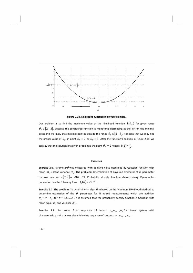
64
L
2
12 L
03 L
Figure 2.18. Likelihood function in solved example.
Our problem is to find the maximum value of the likelihood function NL for given range
32N . Because the considered function is monotonic decreasing at the left on the minimal
point and we know that minimal point is outside the range 32N , it means that we may find
the proper value of N in point 2N or 3N . After the function’s analysis in Figure 2.18, we
can say that the solution of a given problem is the point 2N where 2
12 L .
Exercises
Exercise 2.6. Parameter was measured with additive noise described by Gaussian function with
mean 0zm and variance z . The problem: determination of Bayesian estimator of parameter
for loss function ,L . Probability density function characterising parameter
population has the following form: ef .
Exercise 2.7. The problem: To determine an algorithm based on the Maximum Likelihood Method, to
determine estimation of the parameter for N noised measurements which are additive:
nn zv , for Nn ,...,2,1 . It is assumed that the probability density function is Gaussian with
mean equal zm and variance z .
Exercise 2.8. For some fixed sequence of inputs Nuuu ,...,, 21 for linear system with
characteristic uy ,it was given following sequence of outputs Nwww ,...,, 21 .
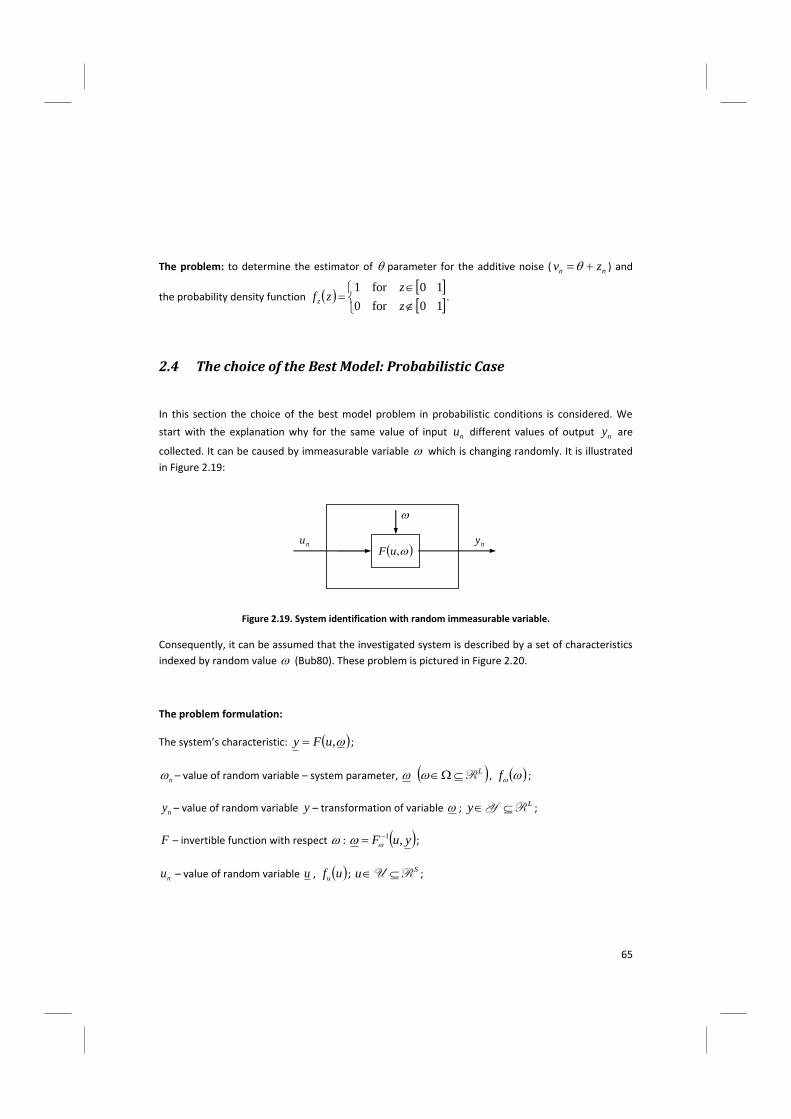
65
The problem: to determine the estimator of parameter for the additive noise ( nn zv ) and
the probability density function
10for0
10for1
z
zzf z .
2.4 The choice of the Best Model: Probabilistic Case
In this section the choice of the best model problem in probabilistic conditions is considered. We
start with the explanation why for the same value of input nu different values of output ny are
collected. It can be caused by immeasurable variable which is changing randomly. It is illustrated
in Figure 2.19:
,uF nu ny
Figure 2.19. System identification with random immeasurable variable.
Consequently, it can be assumed that the investigated system is described by a set of characteristics
indexed by random value (Bub80). These problem is pictured in Figure 2.20.
The problem formulation:
The system’s characteristic: ,uFy ;
n – value of random variable – system parameter, LR , f ;
ny – value of random variable y – transformation of variable ; Ly RY ;
F – invertible function with respect : yuF ,1 ;
nu – value of random variable u , ufu ; Su RU ;
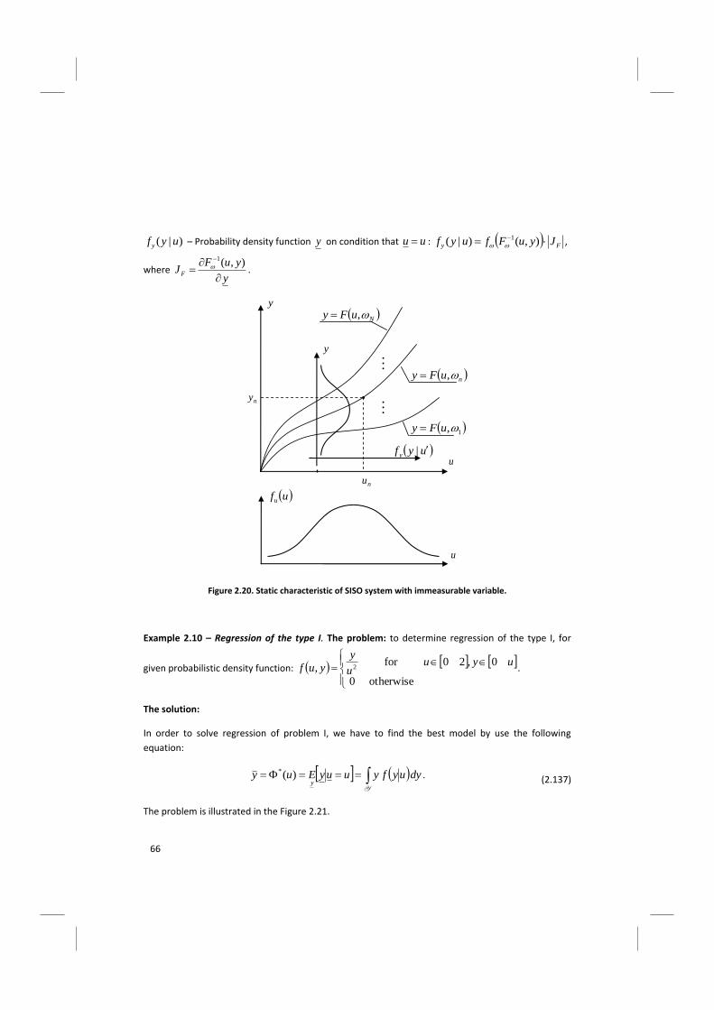
66
)|( uyf y – Probability density function y on condition that uu : Fy JyuFfuyf ),()|( 1
,
where y
yuFJF
),(1
.
Figure 2.20. Static characteristic of SISO system with immeasurable variable.
Example 2.10 – Regression of the type I. The problem: to determine regression of the type I, for
given probabilistic density function:
otherwise0
0,20for, 2
uyuu
y
yuf .
The solution:
In order to solve regression of problem I, we have to find the best model by use the following
equation:
dyuyfyuuyEuyy
Y
)(* . (2.137)
The problem is illustrated in the Figure 2.21.
ufu
u
u
y
NuFy ,
nu
ny
nuFy ,
1,uFy
y
uyf y|
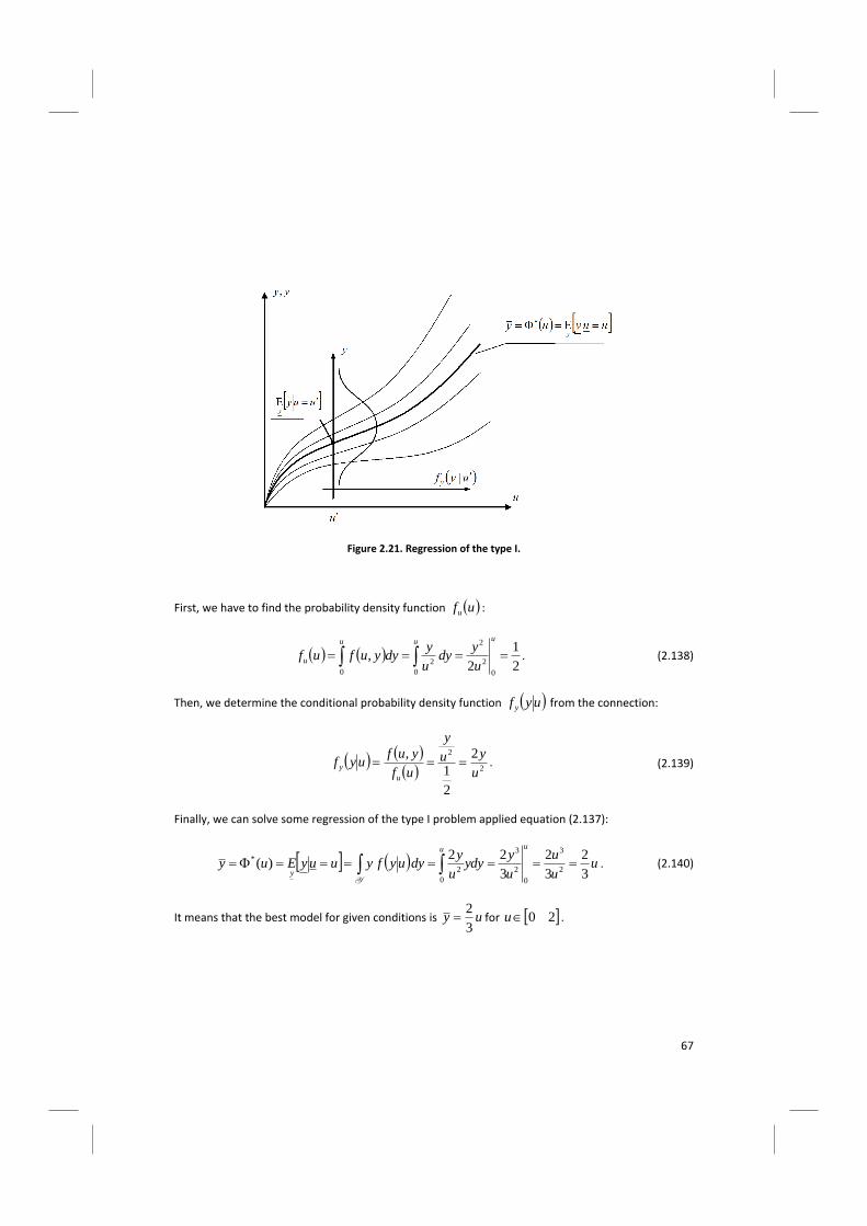
67
Figure 2.21. Regression of the type I.
First, we have to find the probability density function ufu :
2
1
2,
0
2
2
0
2
0
uuu
uu
ydy
u
ydyyufuf . (2.138)
Then, we determine the conditional probability density function uyf y from the connection:
2
2 2
2
1
,
u
yu
y
uf
yufuyf
u
y . (2.139)
Finally, we can solve some regression of the type I problem applied equation (2.137):
uu
u
u
yydy
u
ydyuyfyuuyEuy
uu
y 3
2
3
2
3
22)(
2
3
0
2
3
0
2
* Y
. (2.140)
It means that the best model for given conditions is uy3
2 for 20u .
68
Example 2.11 – Regression of the type II. The problem: to determine regression of the type II for
given conditional probability density function:
otherwise0
0,20for,
2
3uyu
u
y
yuf .
Assume: model 01, uuy and the quadratic performance index
dudyyufuyQ ,,2
UY
.
The solution:
Taking:
ufuyfyuf uy |, , (2.141)
we can rewrite proposed quadratic performance index as:
U
duufuyfuyQ uy |,2
. (2.142)
In order to find an optimal value of the ,we have to solve the following optimization problem (see
lecture 10):
U
duufuuQ u
2* ,minmin
. (2.143)
We have to start with solving regression of the type I problem u* . To be patterned on
calculations from example 2.10, first we have to find the probability density function:
22
,
222
0
3
2
0
3
0
u
u
ydy
u
ydyyufuf
uuu
u . (2.144)
Then, the conditional probability density function (see 2.141) must be determined:
4
3 2
2
,
u
y
uu
y
uf
yufuyf
u
y , (2.145)
and
2
4
6
0
4
3
0
4
*
3
2
3
2
3
22)(
22
uu
u
u
yydy
u
ydyuyfyuuyEuy
uu
y
Y
. (2.146)
69
Then, we can rewrite the performance index Q in the form:
U
duufuuQ u
2
2 ,3
2 . (2.147)
Taking into account, that 2
uufu and 01, uu , we can rewrite (2.147) in the form:
U
duu
uuQ23
22
012 . (2.148)
In order to solve the optimization problem (2.147) we have to consider the following system of
equations:
20* Q . (2.149)
Substituting (2.148) in (2.149) and taking into account that 20: uu RU , we obtain:
2
2
0
2
012 023
2
1*1
0*0
du
uuuQ . (2.150)
In order to find the optimal value of parameters vector , we have to solve the following set of
equations (2.150):
0
3
2
2
12
013
2
2
12
2
0
0*1*2
1
2
0
0*1*2
0
duuuuuQ
duuuuQ
. (2.151)
After a few transformations, we obtain the following equations:
0
3
22
0
0*21*3
duuuu , (2.152)
And
70
0
3
22
0
20*31*4
duuuu . (2.153)
Let us now focus on a connection (2.152):
0
2343
2
03
2
2
0
20*
2
0
31*
2
0
4
2
0
0*21*3
uuu
duuuu
.
(2.154)
Then, we obtain:
1*0*
3
4
3
4 . (2.155)
In the next step, we determine 1* from the equation (2.153):
0
3453
22
0
30*
2
0
41*
2
0
5
uuu
, (2.156)
and then we obtain:
0*1*
3
2
15
16 . (2.157)
Finally, taking (2.155) and (2.157), we obtain such optimal values of parameters vector as:
5
8,
5
4 1*0* . (2.158)
It means, that the best model as regression of the type II for given system is 5
4
5
8, uuy .
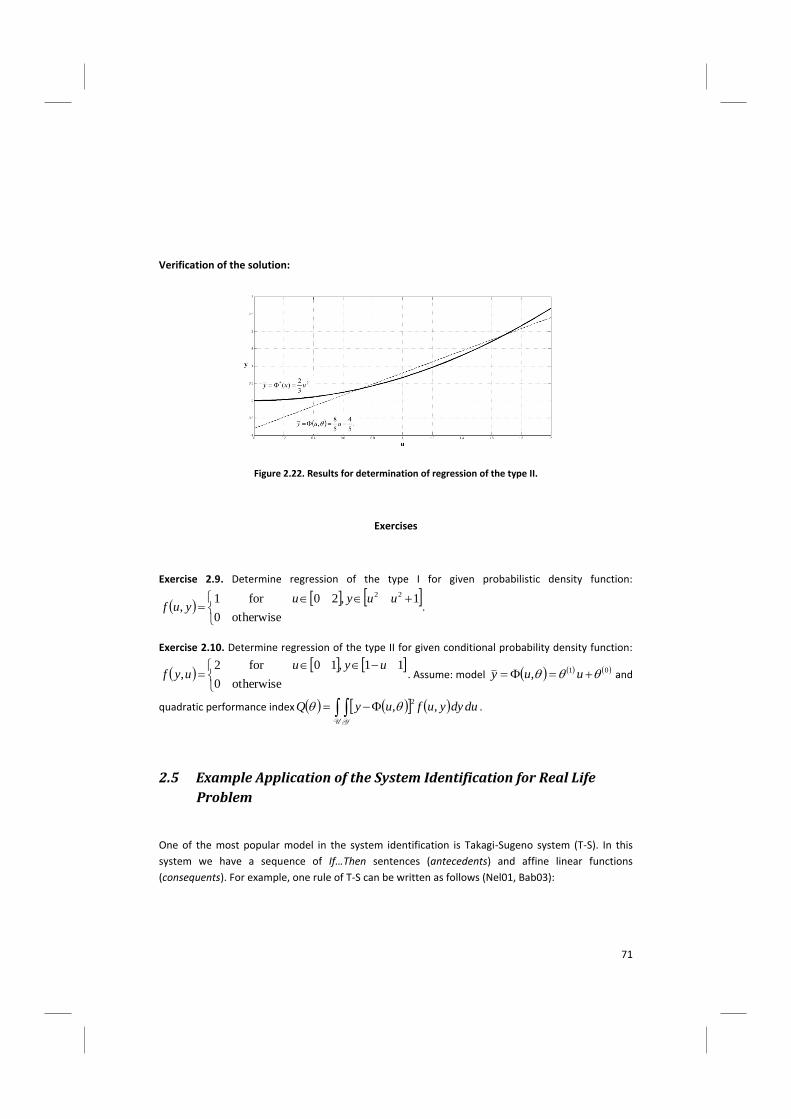
71
Verification of the solution:
Figure 2.22. Results for determination of regression of the type II.
Exercises
Exercise 2.9. Determine regression of the type I for given probabilistic density function:
otherwise0
1,20for1,
22 uuyuyuf .
Exercise 2.10. Determine regression of the type II for given conditional probability density function:
otherwise0
11,10for2,
uyuuyf . Assume: model 01, uuy and
quadratic performance index dudyyufuyQ ,,2
UY
.
2.5 Example Application of the System Identification for Real Life
Problem
One of the most popular model in the system identification is Takagi-Sugeno system (T-S). In this
system we have a sequence of If…Then sentences (antecedents) and affine linear functions
(consequents). For example, one rule of T-S can be written as follows (Nel01, Bab03):
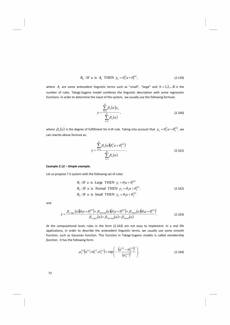
72
0 THEN is IF: k
T
kkkk uyAuR , (2.159)
where iA are some antecedent linguistic terms such as “small”, “large” and Kk ,...2,1 is the
number of rules. Takagi-Sugeno model combines the linguistic description with some regression
functions. In order to determine the input of the system, we usually use the following formula:
K
k
k
K
k
kk
u
yu
y
1
1
, (2.160)
where uk is the degree of fulfillment for k-th rule. Taking into account that 0
k
T
kk uy , we
can rewrite above formula as:
K
k
k
K
k
k
T
kk
u
uu
y
1
1
0
. (2.161)
Example 2.12 – Simple example.
Let us propose T-S system with the following set of rules:
0
3333
0
2222
0
1111
THEN mall is IF:
THEN ormal is IF:
THEN arge is IF:
uySuR
uyNuR
uyLuR
. (2.162)
and
uuu
uuuuuuy
SmallNormaleL
SmallNormaleL
arg
0
13
0
12
0
11arg. (2.163)
At the computational level, rules in the form (2.163) are not easy to implement. In a real life
applications, in order to describe the antecedent linguistic terms, we usually use some smooth
function, such as Gaussian function. This function in Takagi-Sugeno models is called membership
function. It has the following form:
2
2
exp,;s
k
s
k
ss
k
s
k
ss
k
mumu
, (2.164)
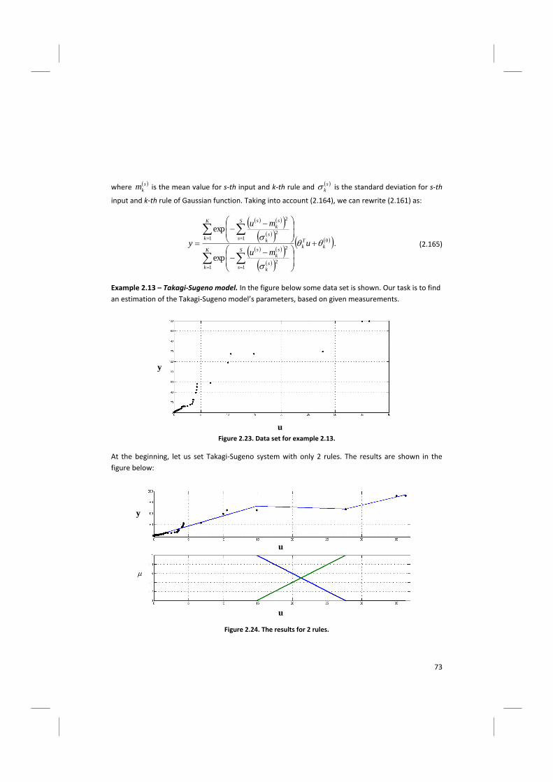
73
where s
km is the mean value for s-th input and k-th rule and s
k is the standard deviation for s-th
input and k-th rule of Gaussian function. Taking into account (2.164), we can rewrite (2.161) as:
0
1 12
2
1 12
2
exp
exp
k
T
kK
k
S
ss
k
s
k
s
K
k
S
ss
k
s
k
s
umu
mu
y
. (2.165)
Example 2.13 – Takagi-Sugeno model. In the figure below some data set is shown. Our task is to find
an estimation of the Takagi-Sugeno model’s parameters, based on given measurements.
Figure 2.23. Data set for example 2.13.
At the beginning, let us set Takagi-Sugeno system with only 2 rules. The results are shown in the
figure below:
Figure 2.24. The results for 2 rules.
y
u
y
u
u
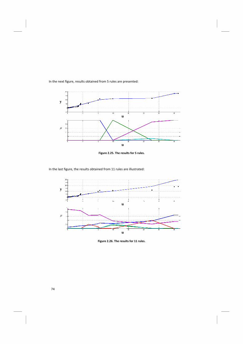
74
In the next figure, results obtained from 5 rules are presented:
Figure 2.25. The results for 5 rules.
In the last figure, the results obtained from 11 rules are illustrated:
Figure 2.26. The results for 11 rules.
y
u
u
y
u
u

75
Bibliography
[Bab03] BABUSKA R., VERBRUGGEN H. ,Neuro-fuzzy methods for nonlinear system identification,
Annual Reviews in Control 27, 2003, pp. 73–85.
[Bis07] BISHOP C.M. ,Pattern Recognition and Machine Learning, Springer 2007.
[Bub80] BUBNICKI Z. ,Identification of Control Plants, PWN-Elsevier, Warszawa-Amsterdam-Oxford-
New York 1980.
*Bro06+ BRONSON R., COSTA G.B. ,Differential equations, Schaum’s Outline Series, McGraw-Hill
Companies, Inc. 2006.
[Che07] CHERKASSKY V., MULIER F. ,Learning form data: concepts, theory, and methods, Wiley, New
Jersey 2007.
[Eyk74] EYKHOFF P. ,System Identification, Parameter and State Estimation, Wiley, New York-London-Sydney 1974.
[Lju99] LJUNG L. ,System identification: Theory for the user, Prince Hall, Englewood Cliffs, New Jersey 1999.
[Nel01] NELLES O. ,Nonlinear system identification. From classical approach to neural networks and fuzzy models, Springer, Berlin, Heidelberg, New York 2001.
[Oga02] OGATA K. ,Modern control engineering, Upper Saddle River, Prentice Hall 2002.
[Vuk03] VUKIC Z., KULJACA L., DONLAGIC D., TESNJAK S., Nonlinear Control Systems, Marcel Dekker, Inc. 2003.
[Świa09+