157

����������������� � �� �������� �� ����� �� ����

http://dx.doi.org/10.7494/drill.2017.34.1.157

Radosław Budzowski*, Damian Janiga*,Robert Czarnota*, Paweł Wojnarowski*

HYDRAULIC FRACTURING OPTIMIZATION FRAMEWORKBASED ON PKN AND CINCO–LEY METHODS**

1. INTRODUCTION

In an era of decreasing number of discoveries of conventional hydrocarbon reser-

voirs, in the global oil and gas industry we can observe growing interest in unconven-tional resources. Conducting effective production from this type of reservoirs is associat-

ed with carrying out the intensification processes of production, among which hydraulic

fracturing is the most popular. Several technological parameters are crucial in caseof process effectiveness. The shape of the fracture is difficult to predict due to the local

inhomogeneity of the reservoir. In the development projects of unconventional resources,

characterized by the presence of significant contrasts of reservoir parameters, the geo-metry of the fracture can be successfully described by simplified mathematical models,

and evaluate the effectiveness of fracturing can be based on analytical methods [13].

Production intensification treatments significantly effect on the physical properties ofthe near well zone, thereby increasing the productivity of the well. The effectiveness

of such treatments can be assessed by analyzing the basic production parameters and

compare the production capacity before and after treatment. Methods of determinationof the effectiveness of the stimulation treatment include analytical and numerical

methods [14]. Numerical methods required high quality and quantity data, therefore

simple analytical methods like Cinco–Lay equivalent skin calculation can be successfulused. Until the 90s of the twentieth century, 2D models were used in modeling of hydraulic

* AGH University of Science and Technology, Faculty of Drilling, Oil and Gas, Krakow, Poland** Paper prepared within the statutory research program of the Faculty of Drilling, Oil and Gas,

AGH University of Science and Technology No. 11.11.190.555

158

fracturing. Currently, specialists are increasingly using 3D models, which, due to its com-plexity, are more difficult to use. Therefore, the 2D models are still used, while beingsimple and in many cases a sufficient approximation of the actual geometry of the frac-ture [2]. In order to describe the geometry of the fracture, PKN model was used [9, 10].This model assumes a constant fracture height, regardless of the distance from the axis ofthe wellbore. The fracture width is a function of the distance from the horizontal axis,and adopts an elliptical outline. The maximum opening of the fracture occurs at theinjection site fracturing fluid. The fracture width in the section plane is proportionalto the net pressure which is defined as the pressure in the fracture decreased by the valueof the stresses directed perpendicularly to the plane of the fracture. This model is used insituations where the length of the wing of the fracture is much higher than its height [6].This paper concerns the various optimization methods, which allows the selection ofappropriate parameters of fracturing technology in terms of maximizing the net valueof the project. Optimization is a very important engineering tool that allows to achievebetter results of hydraulic fracturing at relatively low cost. Optimization algorithm wasdeveloped based on two-dimensional PKN model and analytical method for assessingthe effectiveness of Cinco–Lay.

2. MATHEMATICAL MODELOF HYDRAULIC FRACTURING EFFECTIVENESS

In case of high contrast of vertical stress in reservoir, fracture geometry can be suc-cessfully described by simplifying Perkins and Kern model. PKN model like other 2D’sassumes constant fracture height in reservoir. The net pressure in fracture defined asdifference between pressure in fracture and reservoir stress in perpendicular fracturedirection and is given by [1]:

[ ]

13 4

432 '

MPainet f

f

Q Ep x

h

⎛ ⎞⋅μ ⋅ ⋅⎜ ⎟= ⋅⎜ ⎟π ⋅⎝ ⎠

(1)

where:pnet – net pressure [MPa],

xf – length of the wing of fracture [m],Qi – injection rate corresponding to one side of the fracture [m3/s],E′ – plane strain modulus [MPa],hf – height of the fracture [m],μ – viscosity of fracturing fluid [Pa·s].

159

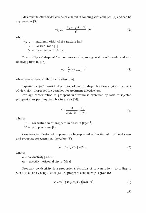
Maximum fracture width can be calculated in coupling with equation (1) and can beexpressed as [3]:

( ) [ ],max1

mnet ff

p hw

G

⋅ ⋅ − ν= (2)

where:wf,max – maximum width of the fracture [m],

ν – Poisson ratio [–],G – shear modulus [MPa].

Due to elliptical shape of fracture cross section, average width can be estimated withfollowing formula [13]:

[ ],max m4f fw wπ= ⋅ (3)

where wf – average width of the fracture [m].

Equations (1)–(3) provide description of fracture shape, but from engineering pointof view, flow properties are curtailed for treatment effectiveness.

Average concentration of proppant in fracture is expressed by ratio of injectedproppant mass per simplified fracture area [14]:

2kg

2 mf f

MC

x h⎡ ⎤= ⎢ ⎥⋅ ⋅ ⎣ ⎦

(4)

where:C – concentration of proppant in fracture [kg/m2],M – proppant mass [kg].

Conductivity of selected proppant can be expressed as function of horizontal stressand proppant concentration, therefore [3]:

( ) [ ], mD mhf Cω = σ ⋅ (5)

where:ω – conductivity [mD·m],σh – effective horizontal stress [MPa].

Proppant conductivity is a proportional function of concentration. According toSun J. et al. and Zhang J. et al [12, 15] proppant conductivity is given by:

( ) ( )[ ], mD mb h bC Cω = α ⋅ϖ σ ⋅ (6)

160

Coefficient of proportionality is equal to ratio between given concentration (C) andbase concentration (Cb) which is used to determine proppant conductivity in horizontalstress range. Proppant conductivity curves for different concentration (Cb, 0.5Cb and 2Cb)are presented in Figure 1.

Fig. 1. Proppant conductivity vs. stress

The relationship between conductivity and permeability of proppant [3]:

[ ] mDff

kwω= (7)

where kf – permeability of the fracture [mD].

The permeability of the fracture allows to calculate the dimensionless fracture con-ductivity [3]:

[ ] –f ffD

f

k wc

k x

⋅=

⋅(8)

where:cfD – dimensionless fracture conductivity [–],

k – permeability of the reservoir [mD].

Using the analytical methodology of Cinco–Lay, we can estimate the value of theequivalent skin effect after fracturing treatment using following formula [3]:

[ ]2

2 31.65 0.328 0.11

ln –1 0.18 0.064 0.005

wf

f

r u us

x u u u

⎛ ⎞ − ⋅ + ⋅= +⎜ ⎟⎜ ⎟ + ⋅ + ⋅ + ⋅⎝ ⎠(9)

�

�

�

�

�

�

161

where:rw – well radius [m],sf – equivalent skin effect [–].

( ) [ ]ln –fDu c= (10)

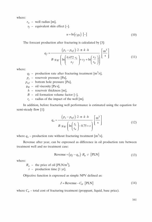
The forecast production after fracturing is calculated by [3]:

( ) 32 m

s0.472ln ln

z wff

feR f

f w

p p k hq

xrB s

x r

− ⋅ ⋅ π ⋅ ⋅ ⎡ ⎤= ⎢ ⎥

⎢ ⎥⎛ ⎞⎛ ⎞ ⎣ ⎦⎛ ⎞⋅⎜ ⎟⋅μ ⋅ + +⎜ ⎟ ⎜ ⎟⎜ ⎟⎜ ⎟⎝ ⎠⎝ ⎠⎝ ⎠

(11)

where:qf – production rate after fracturing treatment [m3/s],pz – reservoir pressure [Pa],

pwf – bottom hole pressure [Pa],μR – oil viscosity [Pa·s],

h – reservoir thickness [m],B – oil formation volume factor [–],re – radius of the impact of the well [m].

In addition, before fracturing well performance is estimated using the equation forsemi-steady flow [1]:

( ) 32 m

sln 0.75

z wfo

eR

w

p p k hq

rB s

r

− ⋅ ⋅ π ⋅ ⋅ ⎡ ⎤= ⎢ ⎥

⎢ ⎥⎛ ⎞⎛ ⎞ ⎣ ⎦⋅μ ⋅ − +⎜ ⎟⎜ ⎟⎜ ⎟⎝ ⎠⎝ ⎠

(12)

where qo – production rate without fracturing treatment [m3/s].

Revenue after year, can be expressed as difference in oil production rate betweentreatment well and no treatment case:

( ) [ ]Revenue PLNf o oq q R t= − ⋅ ⋅ (13)

where:Ro – the price of oil [PLN/m3],

t – production time [1 yr].

Objective function is expressed as simple NPV defined as:

[ ]Revenue PLNtrJ C= − (14)

where Ctr – total cost of fracturing treatment (proppant, liquid, base price).

162

Optimization problem involves maximization function J by changing decision vari-able: fracture half length (xf) and proppant mass (M) with respect of specific contrast:

* 2max(Revenue (u) ( )), trJ C u u= − ∈ℜ (15)

Tfu x M⎡ ⎤= ⎣ ⎦ (16)

With respect to constraints of solution space:

min maxf f fx x x≤ ≤ (17)

min maxM M M≤ ≤ (18)

3. OPTIMIZATION METHODS

Optimization method for presented engineering problem based on two populationtype algorithms, which mimic nature mechanism principles and concepts. First one baseson wolf pack haunting mechanism – grey wolf optimizer, and the second one mimicswarm intelligence – particle swarm optimization. Due to analytical form of relationbetween variables and objective function, gradient optimization is used. Gradientmethods are a directional search, where direction of updating variables depends onobjection function gradient with respect to variables. The main disadvantage of gradientalgorithm is its local search aspect. In case of non-smooth objective function, gra-dient methods converge to nearest start point local optimum. Therefore global optimiza-tion methods like GWO or PSO are used to evaluate optimal fracture design parameters.All of proposed algorithms were implemented in Matlab software.

Grey wolf optimizer – GWO

GWO algorithm was developed by Mirjalili [7]) inspiring by grey wolves pack. Algo-rithm based on leadership hierarchy and hunting mechanism of wolves in nature. Similarto nature equivalent algorithm base on four types of possible solution:

– alpha – which is the best solution.– beta and delta – the second and third best solution,– gamma – the rest of possible solutions.

Possible solutions (alpha, beta, delta and gamma) change position in search spacewith very strict haunting rules, detailed in Muro [8]. Firstly tracking, chasing andapproaching the prey. Secondly pursuit, encircling and harassing the prey until it stopsmoving and the last step is attack the prey. Detailed mathematical description of GWOalgorithm was presented in origin paper [7].

163

Particle swarm optimization – PSO

The PSO algorithm is a based stochastic optimization procedure developed byKennedy and Eberhardt [4]. The algorithm mimics the social behaviors exhibitedby swarms of animals. In the PSO algorithm, a point in the research space is calleda particle. The collection of particles in a given iteration is referred as the swarm.PSO algorithm is used for problems where objective function is non-smooth, discon-tinuous and non-differentiable with non-linearity related parameters [5]. Change ofparticle position in space of optimization problem is updated with respect of inertia,cognitive and social component. The inertia component provides a degree of continuityin particle velocity from one iteration to the next, while the cognitive component causesthe particle move towards its own previous best position. The social component movesthe particle towards the best particle in its neighborhood. These tree component performdifferent role in optimization. The inertia components enable a broad explorationof search space, while cognitive and social components narrow search towards the pro-mising solution found up to the current iteration. The main advantages of PSO are:intensiveness to scaling design variables, simple implementation, ease parallelism, deriv-ative free and efficient global search. Authors tested possibility of implementation PSOalgorithm to solve complex engineering problem related to well placement and control tomaximize CO2 trapping, where detailed description of algorithm can be found [11].

Gradient optimization

Gradient optimization using in this paper based on Newton method which includehessian of objective function to improve solution. Gradient of objective function can becalculated analytically or numerically depending on problem type. Subject of numericalcalculations need an additional function evaluation.

4. CASE STUDY

For case study following engineering problem was stated: The wellbore W-1 piercedsandstone layer located at a depth of 3100 m. The thickness of the hydrocarbon-bearingrock is 15 m. These sandstones have Poisson ratio equal to 0.27, the Young’s modulusis 8.5 GPa and permeability 5mD. Average formation pressure is 24 MPa, and a bottomhole pressure 22 MPa. Skin effect before the treatment is equal to 10. The viscosityof the oil is 5 cP, and the volume ratio of oil 1.101. The radius of the impact of wellis 1000 m, and the wellbore radius is 0.2 m. The company performing hydraulic frac-turing has pumped storage units with a capacity of 0.2 m3/s. During the procedure,it is planned to create the fracture with a height of 15 m. Leak off coefficient is equal0.0002 m/s0.5.

164

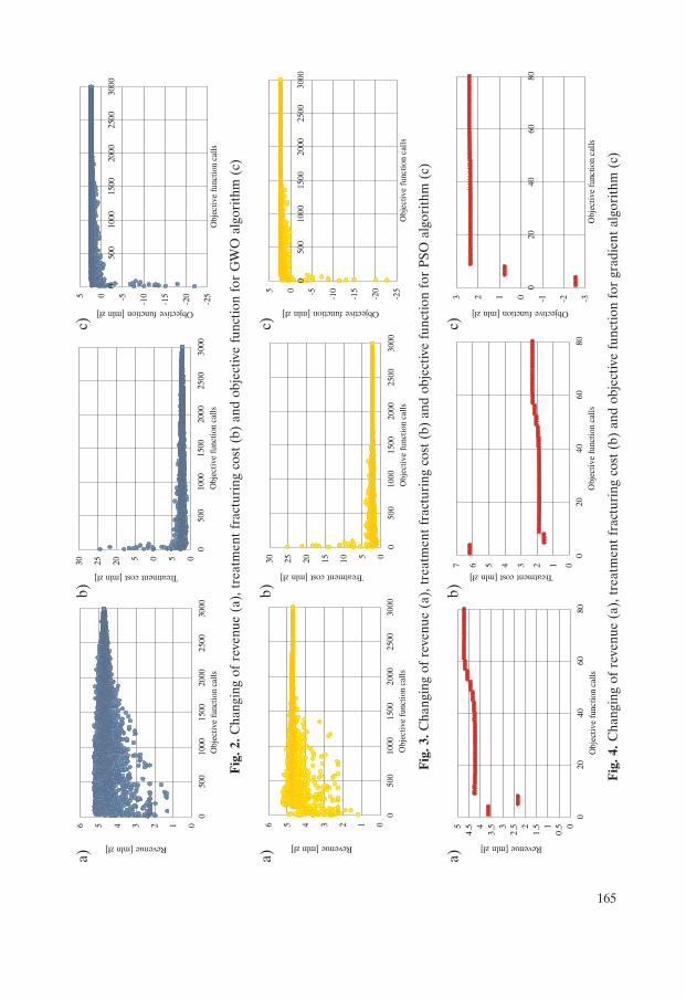
For population algorithm (GWO and PSO) 30 generation per 10 individual simula-tions were performed to converge. Stopping criteria for gradient algorithm were metwhen function gradient decreased to zero. Results of optimization in case of lengthof fracture wing and proppant mass are presented in table 1. The results of the optimiza-tion using GWO, PSO and gradient method are similar. The difference in the fracturewing length is about 3 cm. This value can be neglected, because the actual length of thefracture depends on the stress distribution in the reservoir and engineer is not able toestimate the fracture length with such precision. According to Table 1, GWO methodyielded the greatest value of the fracture length: 175.5125. The values obtainedby the PSO and gradient methods are almost identical (the difference below 1 cm).The similarity of these two methods is even more pronounced when we look at the valuesof the proppant weight. Both methods yielded results about 116 886 kg (difference belowthan 1 kg). The mass of proppant in the GWO method is equal to 11 7009.2 kg. The differ-ence is noticeable – approximately 125 kg. Using the expert knowledge fracture wouldhave 112 m of length and service would use 180 000 kg of proppant material. Changingof revenue, treatment cost and objective function value are presented in Figures 2–4,for GWO, PSO and gradient algorithm respectively.

Table 1

Optimal fracture design parameters and comparison with expert knowledge

During optimization using GWO and PSO methods 3000 calls were conducted.Referring to Figure 2 and 3, it can be observed, that after about 1500 calls revenue andtreatment cost in PSO method are beginning to stabilize at a certain level. In the GWOmethod, substantially to the last calls fluctuations in values are observed – this is particu-larly evident looking at the first graph (Fig. 2). The PSO method is characterized bya smaller values dispersion during operation of the algorithm. Graphs for gradientmethod look differently. It should be note that in this method only 80 calls were used.After 10 calls value of the objective function started stabilization (Fig. 5). It is worthto mention, that on the graphs with treatment cost, value dispersion ranges from 0 to25 million PLN (GWO and PSO optimization methods). Using gradient method weobserved this dispersion from 1.5 to 6.1 million PLN.

GWO PSO Gradient Expert

knowledge

xf [m] 175.5125 175.4907 175.4895 112

M [kg] 117 009.2 116 885.4 116 886.2 180 000

165

Fig

. 4. C

hang

ing

of r

even

ue (

a), t

reat

men

t fr

actu

ring

cos

t (b

) an

d ob

ject

ive

func

tion

for

grad

ient

alg

orith

m (

c)

Fig

. 2. C

hang

ing

of r

even

ue (

a), t

reat

men

t fr

actu

ring

cos

t (b

) an

d ob

ject

ive

func

tion

for

GW

O a

lgor

ithm

(c)

Fig

. 3. C

hang

ing

of r

even

ue (

a), t

reat

men

t fr

actu

ring

cos

t (b

) an

d ob

ject

ive

func

tion

for

PSO

alg

orith

m (

c)

Revenue [mln zł]

Treatment cost [mln zł]

Objective function [mln zł]

Revenue [mln zł]

Treatment cost [mln zł]

Objective function [mln zł]

Revenue [mln zł]

Treatment cost [mln zł]

Objective function [mln zł]

a)b)

c)

a)b)

c)

a)b)

c)

166

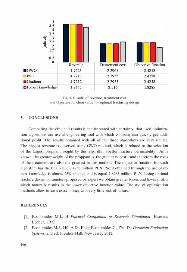
Fig. 5. Results of revenue, treatment costand objective function value for optimal fracturing design

5. CONCLUSIONS

Comparing the obtained results it can be stated with certainty, that used optimiza-tion algorithms are useful engineering tool with which company can quickly get addi-tional profit. The results obtained with all of the three algorithms are very similar.The biggest revenue is observed using GWO method, which is related to the selectionof the largest proppant weight by this algorithm (better fracture permeability). As isknown, the greater weight of the proppant is, the greater is cost – and therefore the costsof the treatment are also the greatest in this method. The objective function for eachalgorithm has the final value 2.4258 million PLN. Profit obtained through the use of ex-pert knowledge is almost 25� smaller and is equal 1.8285 million PLN. Using optimalfracture design parameters proposed by expert we obtain greater losses and lower profitswhich naturally results in the lower objective function value. The use of optimizationmethods allow to earn extra money with very little risk of failure.

REFERENCES

[1] Economides M.J.: A Practical Companion to Reservoir Stimulation. Elsevier,Leoben, 1992.

[2] Economides M.J., Hill A.D., Ehlig-Economides C., Zhu D.: Petroleum ProductionSystems, 2nd ed. Prentice Hall, New Jersey 2012.

167

[3] Economides M.J., Nolte K.G.: Reservoir Stimulation, 3rd ed. John Wiley & Sons,New York 2000.

[4] Eberhart R., Kennedy J.: A new optimizer using particle swarm theory, in: MicroMachine and Human Science, MHS ’95, Proceedings of the Sixth InternationalSymposium on, 1995, pp. 39–43.

[5] Floreano D., Mattiussi C.: Bio-inspired artificial intelligence: theories, methods, andtechnologies. MIT Press, 2008.

[6] Guo B., Lyons W.C., Ghalambor A.: Petroleum Production Engineering. ElsevierScience & Technology Books, 2007.

[7] Mirjalili S., Mirjalili S.M., Lewis A.: Grey Wolf Optimizer. Advances in Engi-neering Software, 69, 2014, pp. 46–61, ISSN 0965-9978.

[8] Muro C., Escobedo R., Spector L., Coppinger R.: Wolf-pack (Canis lupus) huntingstrategies emerge from simple rules in computational simulations. Behavioural Pro-cesses, 88 (3), 2011, pp. 192–197, ISSN 0376-6357.

[9] Nordgen R.P.: Propagation of a vertical hydraulic fracture. SPE Journal, August1972.

[10] Perkins T.K., Kern L.R.: Widths of Hydraulic Fractures. JPT, September 1961.[11] Stopa J., Janiga D., Wojnarowski P., Czarnota R.: Optimization of well placement

and control to maximize CO2 trapping during geologic sequestration. AGH Drilling,Oil, Gas, vol. 33, No. 1, 2016, pp. 93–104.

[12] Sun J., Gamboa E.S., Schechter D., Rui Z.: An integrated workflow for characte-rization and simulation of complex fracture networks utilizing microseismic and hori-zontal core data. Journal of Natural Gas Science and Engineering, 34, 2016,pp. 1347–1360.

[13] Valko P., Economides M.J.: Hydraulic Fracture Mechanics. John Wiley & Sons,New York 1997.

[14] Wojnarowski P.: Metody modelowania i oceny efektywności zabiegów szczelinowaniahydraulicznego skał złożowych w odwiertach naftowych. Wydawnictwa AGH, Kra-ków 2013.

[15] Zhang J., Kamenov A., Zhu D., Hill A.D.: Laboratory Measurement of HydraulicFracture Conductivities in the Barnett Shale. International Petroleum TechnologyConference, Texas A&M University, 2013.