CER

N-T

HES

IS-2

018-

110

//20

18

na kierunku Fizyka Technicznaw specjalnosci Fizyka i Technika Jadrowa

Optimalisation of track reconstruction using vertex detector in theNA61/SHINE experiment

Wojciech BrylinskiNumer albumu 261553

opiekundr inz. Dariusz Tefelski

opiekun zewnetrznydr hab. Paweł Staszel

WARSZAWA 2018

Acknowledgements

I would like to express enormous gratitude to my Supervisors: Dariusz Tefelski and Paweł Staszel,for the constant support and for guiding me through the whole analysis. Thanks to you, I reallyenjoyed working on this thesis. Thank you!

I also wish to thank very much all the people from the NA61/SHINE Collaboration. I had manyopportunities to spend a wonderful time in the experiment, meeting very interesting scientists andhaving many discussions – not only about physics.

I am thankful to the NA61/SHINE group at the Faculty of Physics, Warsaw University ofTechnology, especially to Katarzyna Grebieszkow for creating warm and family atmosphere in thegroup. Special thanks to the NA61/SHINE DCS group: Tobiasz Czopowicz and Bartosz Maksiak(thanks to you I joined the NA61/SHINE experiment!). It is a fantastic experience to have even asmall input to the Detector Control System.

Finally, I would like to express my gratitude to all my friends which I met during the studies; Rafał,Monika, Justyna, Ewa, Maciek and many others. With many of you I spent a great time while beingat CERN.

Last but not least, I would like to thank my family; my parents and my brothers: Piotr, Krzysztofand Łukasz. Especially, I wish to thank my brother and best friend – Paweł Brylinski with whom I wasliving for three years of my studies and who unfortunately passed away in May 2016. I dedicate thiswork to him.

Abstract

Title of the thesis: Optimalisation of track reconstruction using vertex detector in theNA61/SHINE experiment

The main result of this thesis shows the first direct measurement of open charm hadrons (D0 andD0) in the collisions of nuclei at the top energy of Super Proton Synchrotron (SPS). It was obtainedfrom the data collected by the NA61/SHINE experiment and is the final result of the feasibility studiesof new NA61/SHINE physics programme. The programme of charm measurements was motivatedby the following questions:◾ What is the mechanism of open charm production?◾ How does the onset of deconfinement impact open charm production?◾ How does the formation of quark-gluon plasma impact J/ψ production?To answer these questions, one need to know the mean number of charm quark pairs ⟨cc⟩ producedin a full phase space in heavy-ion collisions. Up to now, such a data does not exist and NA61/SHINEstarted the corresponding measurements in December 2016. Because of very short lifetime of opencharm hadrons, a micro vertex detector is needed to perform the measurement. In December 2016,the Small-Acceptance Vertex Detector (SAVD) was installed and the first data for Pb+Pb collisionsat 150A GeV/c were collected. The Vertex Detector will be upgraded during the Long Shutdown 2 atCERN (2019-2020).

The first step of the data analysis was reconstruction. Two algorithms implemented as a part ofthis thesis were used: the algorithm of silicon sensors alignment and the algorithm of VD-TPC trackmatching. The geometry corrections were calculated in a way to minimise the distances betweenclusters and fitted tracks. The data collected without magnetic field were used, because then clusterscreated by one particle should lie on the straight line. The final corrections improved the spatialclusters resolution up to 20%. The track matching was done using the method via interpolation. Atfirst the tracks were refitted to primary vertex reconstructed by Vertex Detector (for primary tracks)or to VD cluster from second station (for secondary tracks) and then interpolated to VD stations inorder to collect the matching clusters.

The implemented algorithms were tested on the analysis of K0s signal. The signal was

successfully observed but the analysis showed the calibration problem of a part of the collectedcollisions. Thus, for the final analysis only properly calibrated data were used. As the most importantresult, the invariant mass distribution of reconstructed secondary tracks was obtained, assuming thepion and kaon masses. It shows the indication of D0 and D0 signal reconstructed from the decaychannel: D0

→ π++K−. This result allowed to validate the measurement concept and confirmed that

NA61/SHINE is able to measure open charm hadrons.

Keywords:CERN, NA61/SHINE, quark-gluon plasma, vertex detector, open charm

(podpis opiekuna naukowego) (podpis dyplomanta)

Streszczenie

Tytuł pracy: Optymalizacja rekonstrukcji sladów czastek z wykorzystaniem detektorawierzchołka w eksperymencie NA61/SHINE

Głównym wynikiem ponizszej pracy magisterskiej jest pierwszy bezposredni pomiar otwartegopowabu (D0 i D0) w zderzeniach ciezkich jonów przy energiach akceleratora Super ProtonSynchrotron (SPS) w osrodku CERN. Został on uzyskany z analizy danych zebranych przezeksperyment NA61/SHINE i stanowi koncowy wynik studium wykonalnosci przyszłego programufizycznego tegoz eksperymentu. Nowy program fizyczny motywowany jest trzema głównymipytaniami:◾ Jaki jest mechanizm produkcji otwartego powabu?◾ Jak efekt uwolnienia kwarków wpływa na produkcje otwartego powabu?◾ Jak wytworzenie plazmy kwarkowo-gluonowej wpływa na produkcje mezonów J/ψ?Aby udzielic odpowiedzi na powyzsze pytania, niezbedna jest znajomosc sredniej krotnosci parpowabnych kwarków ⟨cc⟩ produkowanych w pełnej przestrzeni fazowej, w zderzeniach ciezkichjonów. Dotychczas takie dane nie były dostepne. Ze wzgledu na bardzo krótki czas zycia hadronówz otwartym powabem, do ich pomiaru niezbedny jest precyzyjny detektor wierzchołka. W grudniu2016 zainstalowano detektor wierzchołka małej akceptancji (Small-Acceptance Vertex Detector –SAVD) i przy jego pomocy zebrano pierwsze dane dla zderzen Pb+Pb przy pedzie wiazki 150AGeV/c.

Pierwszym etapem analizy zebranych danych jest rekonstrukcja. W tym celu wykorzystano 2algorytmy zaimplementowane w ramach omawianej pracy; algorytm pozycjonowania krzemowychsensorów oraz algorytm łaczenia sladów czastek zrekonstruowanych przy pomocy detektorawierzchołka ze sladami z innych poddetektorów spektrometru NA61/SHINE. Korekcje na połozeniasensorów, obliczono minimalizujac odległosci miedzy zrekonstruowanymi sladami oraz zebranymiklastrami. Po zastosowaniu korekcji, rozdzielczosc połozenia klastrów polepszyła sie do 20%. Dołaczenia zrekonstruowanych sladów wykorzystano metode bazujaca na interpolacji. W pierwszymetapie slad jest ponownie dopasowywany uwzgledniajac połozenie wierzchołka zrekonstruowanegoz detektora wierzchołka (w przypadku sladów pierwotnych) lub połozenie klastra z drugiej stacjidetektora wierzchołka (dla sladów wtórnych). Nastepnie slad jest interpolowany do pozostałychstacji, gdzie dobierane sa pasujace klastry.

Zaimplementowane algorytmy przetestowano na analizie sygnału z rozpadu K0s. Odpowiedni

sygnał został zaobserwowany. Analiza wykazała jednak problemy z kalibracja czesci zebranychdanych. Dlatego, do koncowej analizy wykorzystano tylko dane poprawnie skalibrowane. Jakonajwazniejszy wynik pracy, otrzymano rozkład masy niezmienniczej zrekonstruowanych sladówwtórnych, zakładajac mase pionu i kaonu. Na rozkładzie widoczny jest wyrazny sygnał z rozpadumezonów D0 i D0. Otrzymany wynik potwierdza koncept samego pomiaru, jak równiez zdolnosceksperymentu NA61/SHINE do analizy produkcji otwartego powabu, co jest głównym celemeksperymentu po 2020 roku.

Słowa kluczowe:CERN, NA61/SHINE, plazma kwarkowo-gluonowa, detektor wierzchołka, otwarty powab

(podpis opiekuna naukowego) (podpis dyplomanta)

Oswiadczenie o samodzielnosci wykonania pracy

Wojciech Brylinski

261553Fizyka Techniczna

Oswiadczenie

Swiadomy odpowiedzialnosci karnej za składanie fałszywych zeznan oswiadczam, zeniniejsza praca dyplomowa została napisana przeze mnie samodzielnie, pod opiekakierujacego praca dyplomowa.Jednoczesnie oswiadczam, ze:

◾ niniejsza praca dyplomowa nie narusza praw autorskich w rozumieniu ustawy z dnia 4 lutego 1994roku o prawie autorskim i prawach pokrewnych (Dz.U. z 2006 r. Nr 90, poz. 631 z pózn. zm.) orazdóbr osobistych chronionych prawem cywilnym,

◾ niniejsza praca dyplomowa nie zawiera danych i informacji, które uzyskałem/-am w sposóbniedozwolony,

◾ niniejsza praca dyplomowa nie była wczesniej podstawa zadnej innej urzedowej proceduryzwiazanej z nadawaniem dyplomów lub tytułów zawodowych,

◾ wszystkie informacje umieszczone w niniejszej pracy, uzyskane ze zródeł pisanych ielektronicznych, zostały udokumentowane w wykazie literatury odpowiednimi odnosnikami,

◾ znam regulacje prawne Politechniki Warszawskiej w sprawie zarzadzania prawami autorskimi iprawami pokrewnymi, prawami własnosci przemysłowej oraz zasadami komercjalizacji.

Oswiadczam, ze tresc pracy dyplomowej w wersji drukowanej, tresc pracy dyplomowej zawartej nanosniku elektronicznym (płycie kompaktowej) oraz tresc pracy dyplomowej w module APD systemuUSOS sa identyczne.

Warszawa, dnia 02.08.2018 (podpis dyplomanta)

Oswiadczenie o udzieleniu Uczelni licencji do pracy

Wojciech Brylinski

261553Fizyka Techniczna

Oswiadczam, ze zachowujac moje prawa autorskie udzielam Politechnice Warszawskiejnieograniczonej w czasie, nieodpłatnej licencji wyłacznej do korzystania z przedstawionejdokumentacji pracy dyplomowej w zakresie jej publicznego udostepniania irozpowszechniania w wersji drukowanej i elektronicznej*.

Warszawa, dnia 02.08.2018 (podpis dyplomanta)

∗Na podstawie Ustawy z dnia 27 lipca 2005 r. Prawo o szkolnictwie wyzszym (Dz.U. 2005 nr 164 poz. 1365) Art. 239. oraz

Ustawy z dnia 4 lutego 1994 r. o prawie autorskim i prawach pokrewnych (Dz.U. z 2000 r. Nr 80, poz. 904, z pózn. zm.)

Art. 15a. "Uczelni w rozumieniu przepisów o szkolnictwie wyzszym przysługuje pierwszenstwo w opublikowaniu pracy

dyplomowej studenta. Jezeli uczelnia nie opublikowała pracy dyplomowej w ciagu 6 miesiecy od jej obrony, student, który

ja przygotował, moze ja opublikowac, chyba ze praca dyplomowa jest czescia utworu zbiorowego."

Contents

1 Introduction and motivation 13

2 Heavy-Ion Physics 132.1 Standard Model . . . . . . . . . . . . . . . . . . . . . . . . . . . . . . . . . . . . . . . . . 132.2 Quark-gluon plasma . . . . . . . . . . . . . . . . . . . . . . . . . . . . . . . . . . . . . . 162.3 Phase diagram of strongly interacting matter . . . . . . . . . . . . . . . . . . . . . . . . 17

3 NA61/SHINE experiment and charm measurement 193.1 Current physics programme . . . . . . . . . . . . . . . . . . . . . . . . . . . . . . . . . . 19

3.1.1 Two-dimensional scan of phase diagram . . . . . . . . . . . . . . . . . . . . . . 193.2 Motivation of open charm measurements . . . . . . . . . . . . . . . . . . . . . . . . . . 21

3.2.1 Mechanism of charm production . . . . . . . . . . . . . . . . . . . . . . . . . . . 213.2.2 Charm yield as the signal of deconfinement . . . . . . . . . . . . . . . . . . . . 223.2.3 J/ψ suppression as the signal of deconfinement . . . . . . . . . . . . . . . . . . 23

3.3 Idea of open charm measurements . . . . . . . . . . . . . . . . . . . . . . . . . . . . . . 253.4 NA61/SHINE detector . . . . . . . . . . . . . . . . . . . . . . . . . . . . . . . . . . . . . 27

3.4.1 Small-Acceptance Vertex Detector . . . . . . . . . . . . . . . . . . . . . . . . . . 283.5 NA61/SHINE beyond 2020 . . . . . . . . . . . . . . . . . . . . . . . . . . . . . . . . . . . 29

3.5.1 NA61/SHINE detector upgrades . . . . . . . . . . . . . . . . . . . . . . . . . . . 293.5.2 NA61/SHINE Vertex Detector . . . . . . . . . . . . . . . . . . . . . . . . . . . . . 30

4 Data reconstruction 324.1 Vertex Detector alignment . . . . . . . . . . . . . . . . . . . . . . . . . . . . . . . . . . . 32

4.1.1 Example results . . . . . . . . . . . . . . . . . . . . . . . . . . . . . . . . . . . . . 354.2 VD-TPC track matching via interpolation . . . . . . . . . . . . . . . . . . . . . . . . . . . 36

4.2.1 Refitting TPC track to VD primary vertex . . . . . . . . . . . . . . . . . . . . . . 364.2.2 Track interpolation to VD stations and cluster collection . . . . . . . . . . . . . . 374.2.3 Refitting TPC track to VD clusters . . . . . . . . . . . . . . . . . . . . . . . . . . 384.2.4 Secondary tracks interpolation to VD stations and cluster collection . . . . . . 39

5 Data analysis 405.1 K0

s test signal . . . . . . . . . . . . . . . . . . . . . . . . . . . . . . . . . . . . . . . . . . . 405.2 D0 signal . . . . . . . . . . . . . . . . . . . . . . . . . . . . . . . . . . . . . . . . . . . . . 42

5.2.1 Track cuts . . . . . . . . . . . . . . . . . . . . . . . . . . . . . . . . . . . . . . . . 425.2.2 Invariant mass distributions . . . . . . . . . . . . . . . . . . . . . . . . . . . . . . 445.2.3 Comparison with different method . . . . . . . . . . . . . . . . . . . . . . . . . . 44

6 Conclusions 47

Bibliography 49

List of Figures 53

1. Introduction and motivation

The aim of the work described in this thesis was to find the first indication of D0 and D0

signal in heavy-ion collisions at the Super Proton Synchrotron (SPS) energies from the directmeasurement using new NA61/SHINE Small-Acceptance Vertex Detector. This is the crucial aspectof the feasibility studies of future physics programme of NA61/SHINE. As a part of this thesis, twoalgorithms used for the data reconstruction were implemented; the algorithm of silicon sensorsalignment and the algorithm of VD-TPC track matching via interpolation. Both algorithms weretested on data collected in December 2016 for Pb+Pb collisions at 150A GeV/c. The analysis ofreconstructed data was also prepared and the final result of invariant mass distribution showingD0 and D0 peak was obtained. The result confirms that NA61/SHINE is able to perform the directmeasurement of open charm hadrons, what is the main goal of the new physics programme of theexperiment.

Section 2 describes the basics of Heavy-Ion Physics. At first, the Standard Model is brieflyintroduced. Then purpose of the studies of heavy-ion collisions is discussed. Section 3 introducesthe NA61/SHINE experiment as well as the method of charm measurement. At the beginning,the current physics programme of NA61/SHINE is discussed and then the motivation of futurephysics programme – open charm measurements – is described. In this section also theNA61/SHINE detector is presented as well as the future plans for the upgrades. In Section 4the data reconstruction chain algorithms, which were implemented as a part of this analysis, aredescribed. Section 5 presents the final analysis and results. Finally, the conclusions are presentedin Section 6.

2. Heavy-Ion Physics

2.1 Standard Model

The Standard Model (SM) [1] is the quantum field theory of elementary particles and interactionsbetween them. It was developed in 20th century by the physicists from around the world. Manypredictions obtained from SM were confirmed experimentally. However, the Standard Model is not acomplete theory. Firstly, it does not include the gravitational interaction. Secondly, in SM neutrinosare massless whereas there is an evidence of their mixing. It also does not include the dark matterand dark energy. Moreover, it has at least 19 free parameters which values are not predicted andhas to be measured (for example the particle masses). Nevertheless, it is the most general andadvanced theory ever created.

The Standard Model assumes the existence of 12 elementary particles (quarks and leptons)with half-integer spin – so called fermions, which together with their anti-particles compose thewhole known matter in the Universe. The interactions between particles are carried by bosons – the

13

2.1 Standard Model

particles with integer spin. SM explains three out of four elementary interactions: strong, weak andelectromagnetic. The overall picture of all particles together with their mass, electric charge and spinis presented in Figure 1.

The group of fermions consists of quarks and leptons. There are six flavors of quarks (up, down,charm, strange, top, bottom) and six leptons (electron, electron neutrino, muon, muon neutrino,tau, tau neutrino). All fermions are divided into three families, each containing two quarks and twoleptons. Particles from the first family build the whole stable matter in our Universe. Each quarkcarries color charge (red, green, blue or anti-red, anti-green, anti-blue for anti-quarks) and onlycolor-neutral hadrons (particles build out of quarks) can be observed. Hadrons build out of threequarks are called baryons (qqq) or anti-baryons (qqq) and out of two quarks are called mesons (qq).

The group of bosons include gauge and scalar bosons. According to the Standard Model, thefollowing gauge bosons exist:◾ gluon – the carrier of strong interactions,◾ Z0, W+, W− – responsible for weak interactions,◾ photon – carrier of the electromagnetic interaction.The summary of fundamental interactions is presented in Figure 2. The only fundamental scalarboson predicted by SM is Higgs boson. It is responsible for the masses of all particles. The existenceof Higgs boson was confirmed by ATLAS and CMS experiments at CERN in 2012.

uup

2.2 MeV2/31/2 c

charm

1.27 GeV2/31/2 t

top

173 GeV 2/31/2

ddown

4.7 MeV-1/31/2 s

strange

96 MeV

1/2-1/3 b

bottom

4.2 GeV

1/2-1/3

νeelectronneutrino

<2 eV01/2 νμ

<0.19 MeV01/2 ντ

tauneutrino

<18.2 MeV 01/2

eelectron

0.511 MeV-11/2 μ

muon

105.7 MeV

1/2-1 τ

tau

1.777 GeV

1/2-1

γphoton

0 01

ggluon

0

10

Z91.2 GeV01

weakforce

W80.4 GeV

1±1

weakforce

mass →

spin →charge →

Qua

rks

Lept

ons

I II III

name →

Bosons(forces)

muonneutrino

Fermions(matter)

HHiggs

125 GeV00

0

±

0

Figure 1: The table of all elementary particles included in the Standard Model. Figure from Ref. [2].

14

2.1 Standard Model

Figure 2: The summary of fundamental interactions. Figure from Ref. [3].

The very important part of the Standard Model is Quantum Chromodynamics (QCD) whichdescribes the nature of strong interactions. It assumes the existence of color – additional stateof freedom. It is the analogical property to the electric charge in Quantum Electrodynamics(QED) theory. However, in contrast to photons – carriers of electromagnetic interactions which areelectrically neutral – gluons carry color charge. This fact causes that the force of strong interactionsincrease with the distance between particles. This is the reason why quarks can not exist as freeparticles. When trying to separate two quarks, at some point the provided energy is so high that it ismore beneficial from the energetic point of view to create another pair of quark and anti-quark. Thiseffect is called confinement and is schematically presented in Figure 3. The only way to observequasi-free quarks is to squeeze them and make the distances between them extremely small.Then the quarks interact very weakly and start behaving like free particles. Such an effect is calledasymptotic freedom.

Figure 3: The schematic picture of confinement effect. Figure from Ref. [4].

15

2.2 Quark-gluon plasma

2.2 Quark-gluon plasma

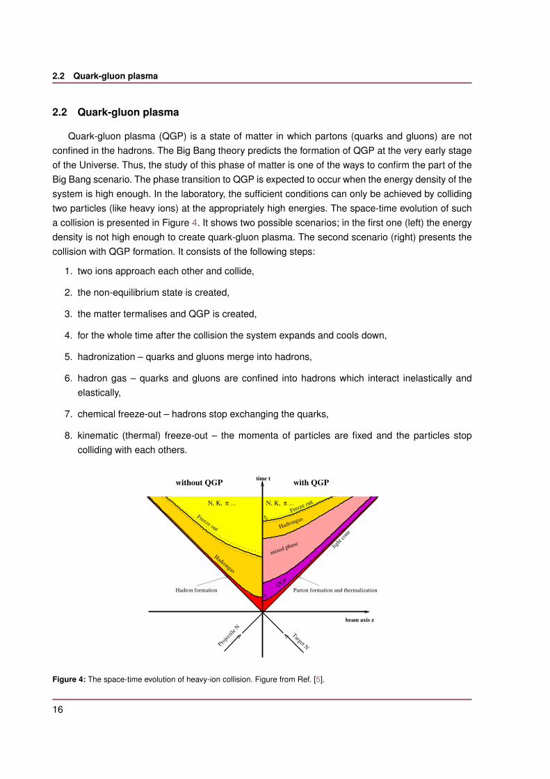
Quark-gluon plasma (QGP) is a state of matter in which partons (quarks and gluons) are notconfined in the hadrons. The Big Bang theory predicts the formation of QGP at the very early stageof the Universe. Thus, the study of this phase of matter is one of the ways to confirm the part of theBig Bang scenario. The phase transition to QGP is expected to occur when the energy density of thesystem is high enough. In the laboratory, the sufficient conditions can only be achieved by collidingtwo particles (like heavy ions) at the appropriately high energies. The space-time evolution of sucha collision is presented in Figure 4. It shows two possible scenarios; in the first one (left) the energydensity is not high enough to create quark-gluon plasma. The second scenario (right) presents thecollision with QGP formation. It consists of the following steps:

1. two ions approach each other and collide,

2. the non-equilibrium state is created,

3. the matter termalises and QGP is created,

4. for the whole time after the collision the system expands and cools down,

5. hadronization – quarks and gluons merge into hadrons,

6. hadron gas – quarks and gluons are confined into hadrons which interact inelastically andelastically,

7. chemical freeze-out – hadrons stop exchanging the quarks,

8. kinematic (thermal) freeze-out – the momenta of particles are fixed and the particles stopcolliding with each others.

beam axis z

Target NProje

ctile

N

light

con

e

without QGP with QGPtime t

Hadrongas

mixed phase

Hadrongas

Freeze out

Hadron formation Parton formation and thermalization

N, K, π ...

Freeze out

N, K, π ...

QGP

τ0

τf

Figure 4: The space-time evolution of heavy-ion collision. Figure from Ref. [5].

16

2.3 Phase diagram of strongly interacting matter

The study of quark-gluon plasma properties is the main motivation of all experiments dedicated forhigh energy heavy-ion collisions. However, such experiments are technically able to register onlythe particles after the hadronization (and freezout) state. It is not possible to measure QGP directlydue to its extremely high temperature, density and very short lifetime. Nevertheless, QGP can bestudied by analysing some observables which are poorly sensitive to the hadronization – so-calledQGP signatures. The most popular are:◾ strangeness enhancement [6] – strangeness is a property of particles expressed as a quantum

number. In heavy-ion collisions stragness is measured by strange hadrons. In quark-gluon plasmaand hadron gas (HG) the carriers of strangeness are different; in QGP strangeness is carriedby strange and anti-strange quarks while for HG the lightest strange hadrons are kaons. Thus,to produce the pair of strange carriers (due to strangeness conservation in strong interactionsthe s quark production must be associated with s quark production) in HG we need more energy(2Mkaon ≈ 2 ⋅500 MeV, 2ms ≈ 2 ⋅100 MeV). Moreover, comparing to the temperature of the phasetransition (Tc ≈ 150 MeV at µB = 0), strange quarks are light particles while kaons are heavy. Allof these properties makes strangeness the perfect variable sensitive to the phase transition fromhadron gas to quark-gluon plasma. Namely, the strangeness production should be increased inQGP scenario.

◾ jet quenching [7] – jets are the collimated streams of particles. Due to the conservation laws theyare usually produced in di-jet structures – as two jets moving in the opposite directions. When di-jetis produced at the surface of QGP volume, one of jets (near-side) propagates normally, whereasthe second one (away-side) propagates through the QGP and because of interactions with densemedium is quenched.

◾ charmonia suppression [8] (see Section 3.2.3) – charmonia are the bound states of charm andanti-charm quarks. The lightest one is the J/ψ meson. When quark-gluon plasma is created, thestrong interactions between produced c and c quarks are screened by quark-gluon soup. Thus,it is less probable for the pair of charm quarks to stay bound and the charmonia production isexpected to be suppressed.

◾ elliptic flow [9, 10] – the fluid-like expansion of dense matter created right after the collision. Themore central collision, the more symmetrically the matter flows. In non-central collisions, the initialspatial anisotropy transfers into the pressure gradients which cause the anisotropic flow and thusthe anisotropy in the momentum space. It can be studied by measuring the Fourier coefficientsin the momentum distribution. The elliptic flow is measured by the second Fourier coefficient –v2 variable. If the energy density of the collision is high enough, v2 scales with the number ofconstituent quarks. This means that, the matter flows at the level of quarks and gluons what isthreated as quark-gluon plasma signature.

2.3 Phase diagram of strongly interacting matter

The existing phases of strongly interacting matter (SIM) can be visualized on the phasediagram. It presents which phase is expected under the defined conditions. The phase diagram

17

2.3 Phase diagram of strongly interacting matter

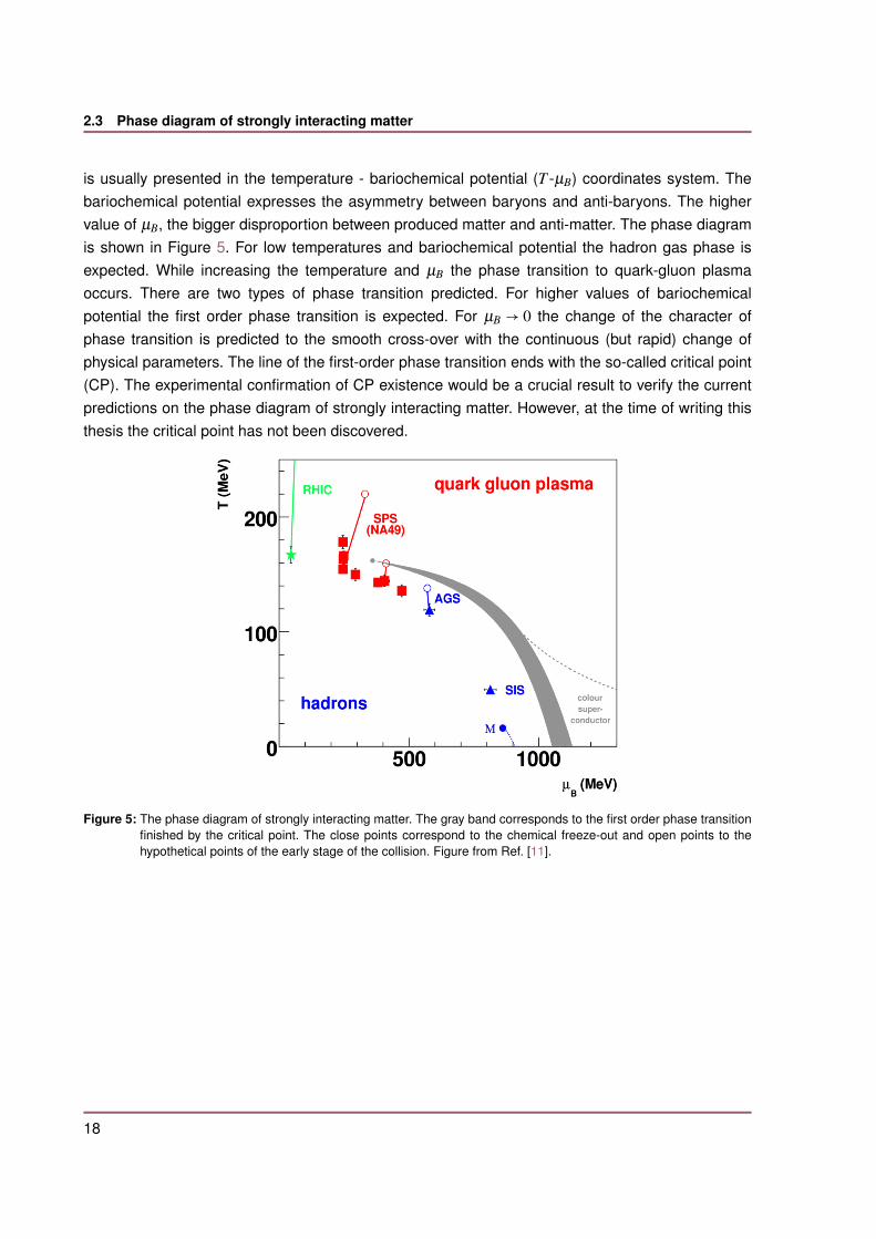
is usually presented in the temperature - bariochemical potential (T -µB) coordinates system. Thebariochemical potential expresses the asymmetry between baryons and anti-baryons. The highervalue of µB, the bigger disproportion between produced matter and anti-matter. The phase diagramis shown in Figure 5. For low temperatures and bariochemical potential the hadron gas phase isexpected. While increasing the temperature and µB the phase transition to quark-gluon plasmaoccurs. There are two types of phase transition predicted. For higher values of bariochemicalpotential the first order phase transition is expected. For µB → 0 the change of the character ofphase transition is predicted to the smooth cross-over with the continuous (but rapid) change ofphysical parameters. The line of the first-order phase transition ends with the so-called critical point(CP). The experimental confirmation of CP existence would be a crucial result to verify the currentpredictions on the phase diagram of strongly interacting matter. However, at the time of writing thisthesis the critical point has not been discovered.

Figure 5: The phase diagram of strongly interacting matter. The gray band corresponds to the first order phase transitionfinished by the critical point. The close points correspond to the chemical freeze-out and open points to thehypothetical points of the early stage of the collision. Figure from Ref. [11].

18

3. NA61/SHINE experiment and charm measurement

SPS Heavy Ion and Neutrino Experiment (SHINE) [12, 13] is a fixed-target experiment operatingat the Super Proton Synchrotron (SPS) at the European Organization for Nuclear Research (CERN).The experiment is dedicated to explore the phase diagram of strongly interacting matter. It is the nextexperiment after NA49 [14] from which SHINE inherited most of the subdetectors. The NA61/SHINEcollaboration consists of 137 physicists from 27 institutions from 12 countries.

3.1 Current physics programme

The physics program of the NA61/SHINE experiment is focused on the following goals:◾ search for the critical point of strongly interacting matter phase diagram,◾ study of the properties of the onset of deconfinement 1,◾ reference measurements for neutrino T2K and Fermilab programme,◾ reference measurements for the Pierre Auger Observatory and KASCADE cosmic-ray

experiments.

3.1.1 Two-dimensional scan of phase diagram

The main physics motivation of the NA61/SHINE experiment is to study the properties of thephase transition between hadronic matter and quark-gluon plasma. Within this program the collisionsof different systems (p+p, p+Pb, Be+Be, Ar+Sc, Xe+La, Pb+Pb) at wide range of beam momenta(13A – 150/158A GeV/c) are registered. Recently, in 2017, Xe+La collisions were recorded. Theoverall summary of collected and planned data is presented in Figure 6.

13 20 30 40 75 150

]c GeV/Abeam momentum [

p+p

p+Pb

Be+Be

Ar+Sc

Xe+La

Pb+Pb

Pb+Pb

colli

ding

nuc

lei

2009/10/11

2012/14/16/17

2011/12/13

2015

2017

182016/

2021-2024

Figure 6: The schematic picture presenting the data collected within system size – beam momentum scan performed byNA61/SHINE. Figure from Ref. [15].

1minimal conditions (for example minimal energy) for which QGP can be created

19

3.1 Current physics programme

The presented system size – beam momentum scan allows to cover the large area on thephase diagram of strongly interacting matter (see Section 2.3), where the critical point is expected.According to one of the QCD lattice calculations (the calculations performed on the discretespace-time lattice) the temperature and bariochemical potential at the critical point are: TCP

= 162±2MeV, µ

CPB = 360±40 MeV [16]. Figure 7 presents the expected (NA61) and measured (NA49) points

of chemical freeze-out on the phase diagram for NA49 and NA61 data. After collecting the data,NA61/SHINE collaboration performs the analyses looking for the signatures of critical point andstudying the phase transition from HG to QGP.

(MeV)B

µ200 300 400 500 600

T (

MeV

)

100

120

140

160

180

200

NA49

p+p

C+CSi+Si

Pb+Pb

NA61 collected data

NA61 future data

p+p

Be+Be

Ar+ScXe+LaPb+Pb

150A GeV/c 13A GeV/c

Figure 7: The coverage of the phase diagram of strongly interacting matter by NA61/SHINE data. Figure from Ref. [15].

20

3.2 Motivation of open charm measurements

3.2 Motivation of open charm measurements

Recently, the physics programme of the NA61/SHINE experiment was extended by themeasurement of open charm hadrons (hadrons composed by one charm or anti-charm quark andlight quarks/anti-quarks) at the CERN SPS energies. It was motivated by three main questions:◾ What is the mechanism of open charm production?◾ How does the onset of deconfinement impact open charm production?◾ How does the formation of quark-gluon plasma impact J/ψ production?In order to answer all of these three questions, the mean multiplicity of charm quarks ⟨cc⟩ producedin a full phase space in heavy-ion collisions has to be known. Up to now, the corresponding datadoes not exist. The acceptance of the NA61/SHINE detector is large enough to extrapolate themeasurements to the full phase space with relatively small uncertainties. This unique feature makesNA61/SHINE the only experiment which is able to perform such a measurement in the near future.In Sections 3.2.1, 3.2.2 and 3.2.3 the questions listed above, which motivate such studies, areillustrated on the examples.

3.2.1 Mechanism of charm production

In Figure 8 the predictions of different models on the mean multiplicity of charm quark pairs ⟨cc⟩produced in central Pb+Pb collisions at 158A GeV/c are presented. The main conclusion from theplot is that the predictions differ by about two orders of magnitude. These very different models couldcoexist up to now because of lack of the experimental data. Therefore, the precise measurement of⟨cc⟩ will narrow the spectrum of theoretical predictions and thus will allow to better understand thecharm quarks and hadrons production mechanism.

Figure 8: Mean multiplicities of charm quark pairs produced in a full phase-space in central Pb+Pb collisions at 158AGeV/c calculated within statistical models (green bars): the Hadron Resonance Gas model (HRG) [17], theStatistical Quark Coalescence model [17] and the Statistical Model of the Early Stage (SMES) [18] as well asdynamical models (blue bars): the Hadron String Dynamics (HSD) model [19, 20], a pQCD-inspired model [21,22] and the Dynamical Quark Coalescence model [23]. Figure from Ref. [24].

21

3.2 Motivation of open charm measurements

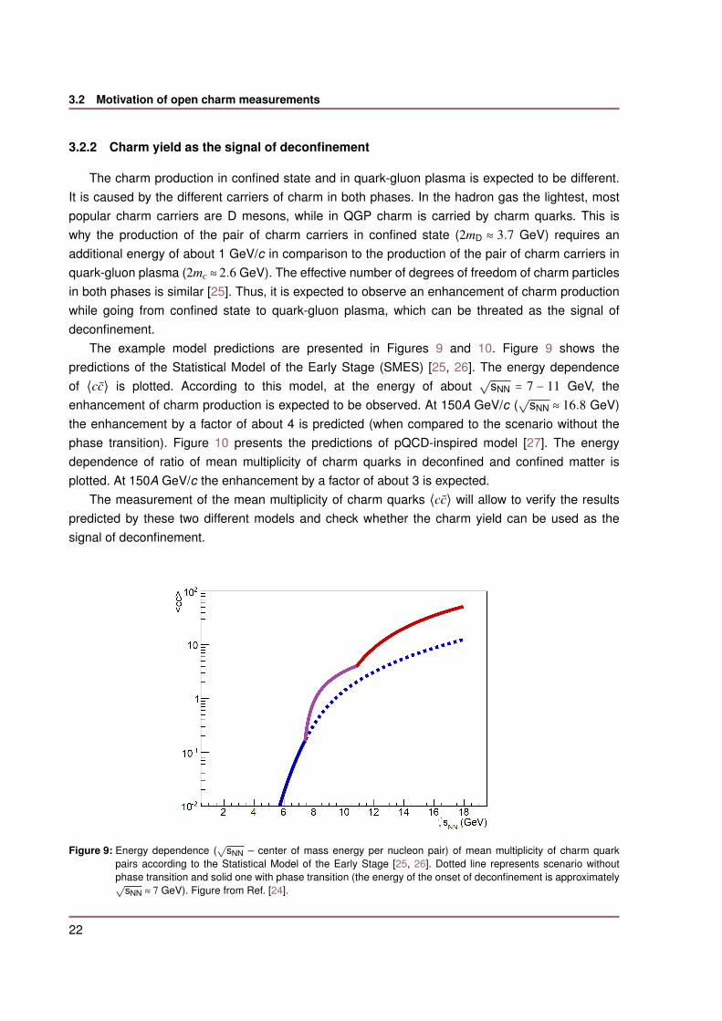
3.2.2 Charm yield as the signal of deconfinement

The charm production in confined state and in quark-gluon plasma is expected to be different.It is caused by the different carriers of charm in both phases. In the hadron gas the lightest, mostpopular charm carriers are D mesons, while in QGP charm is carried by charm quarks. This iswhy the production of the pair of charm carriers in confined state (2mD ≈ 3.7 GeV) requires anadditional energy of about 1 GeV/c in comparison to the production of the pair of charm carriers inquark-gluon plasma (2mc ≈ 2.6 GeV). The effective number of degrees of freedom of charm particlesin both phases is similar [25]. Thus, it is expected to observe an enhancement of charm productionwhile going from confined state to quark-gluon plasma, which can be threated as the signal ofdeconfinement.

The example model predictions are presented in Figures 9 and 10. Figure 9 shows thepredictions of the Statistical Model of the Early Stage (SMES) [25, 26]. The energy dependenceof ⟨cc⟩ is plotted. According to this model, at the energy of about

√sNN = 7 − 11 GeV, the

enhancement of charm production is expected to be observed. At 150A GeV/c (√

sNN ≈ 16.8 GeV)the enhancement by a factor of about 4 is predicted (when compared to the scenario without thephase transition). Figure 10 presents the predictions of pQCD-inspired model [27]. The energydependence of ratio of mean multiplicity of charm quarks in deconfined and confined matter isplotted. At 150A GeV/c the enhancement by a factor of about 3 is expected.

The measurement of the mean multiplicity of charm quarks ⟨cc⟩ will allow to verify the resultspredicted by these two different models and check whether the charm yield can be used as thesignal of deconfinement.

Figure 9: Energy dependence (√

sNN – center of mass energy per nucleon pair) of mean multiplicity of charm quarkpairs according to the Statistical Model of the Early Stage [25, 26]. Dotted line represents scenario withoutphase transition and solid one with phase transition (the energy of the onset of deconfinement is approximately√

sNN ≈ 7 GeV). Figure from Ref. [24].

22

3.2 Motivation of open charm measurements

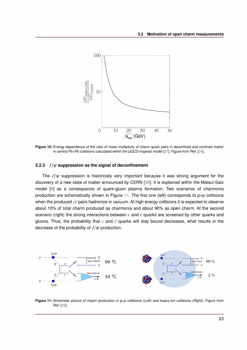
Figure 10: Energy dependence of the ratio of mean multiplicity of charm quark pairs in deconfined and confined matterin central Pb+Pb collisions calculated within the pQCD-inspired model [27]. Figure from Ref. [24].

3.2.3 J/ψ suppression as the signal of deconfinement

The J/ψ suppression is historically very important because it was strong argument for thediscovery of a new state of matter announced by CERN [28]. It is explained within the Matsui-Satzmodel [8] as a consequence of quark-gluon plasma formation. Two scenarios of charmoniaproduction are schematically shown in Figure 11. The first one (left) corresponds to p+p collisionswhen the produced cc pairs hadronize in vacuum. At high energy collisions it is expected to observeabout 10% of total charm produced as charmonia and about 90% as open charm. At the secondscenario (right) the strong interactions between c and c quarks are screened by other quarks andgluons. Thus, the probability that c and c quarks will stay bound decreases, what results in thedecrease of the probability of J/ψ production.

Figure 11: Schematic picture of charm production in p+p collisions (Left) and heavy-ion collisions (Right). Figure fromRef. [29].

23

3.2 Motivation of open charm measurements

The probability of J/ψ production is given by the following formula:

P(cc→ J/ψ) ≡⟨J/ψ⟩⟨cc⟩

≡

σJ/ψσcc

, (1)

where ⟨...⟩ represents mean multiplicities and σ – corresponding cross-sections. Thus, in order tocalculate the probability of a cc pair hadronizing to J/ψ , the data on the mean multiplicity of bothJ/ψ and cc in a full phase space is required. The J/ψ yields were precisely measured by other SPSexperiments (NA38 [30], NA50 [31], NA60 [32]), while ⟨cc⟩ was not measured before – NA61/SHINEstarted the corresponding measurements in 2016.Up to now, in order to analyse very rich J/ψ measurements, the assumption that the mean multiplicityof cc quarks is proportional to the mean multiplicity of Drell-Yan 2 pairs was used [8, 31]:

⟨cc⟩ ∼ ⟨DY ⟩. (2)

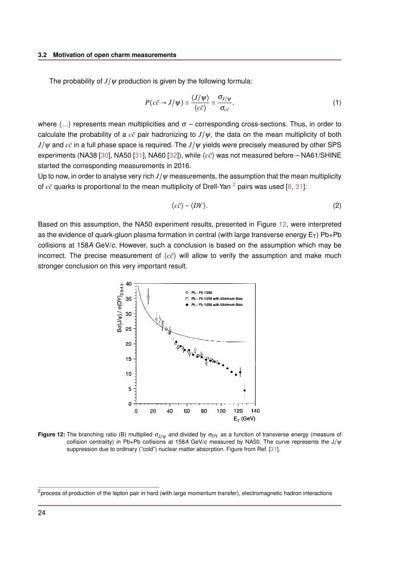
Based on this assumption, the NA50 experiment results, presented in Figure 12, were interpretedas the evidence of quark-gluon plasma formation in central (with large transverse energy ET) Pb+Pbcollisions at 158A GeV/c. However, such a conclusion is based on the assumption which may beincorrect. The precise measurement of ⟨cc⟩ will allow to verify the assumption and make muchstronger conclusion on this very important result.

Figure 12: The branching ratio (B) multiplied σJ/ψ and divided by σDY as a function of transverse energy (measure ofcollision centrality) in Pb+Pb collisions at 158A GeV/c measured by NA50. The curve represents the J/ψsuppression due to ordinary (”cold”) nuclear matter absorption. Figure from Ref. [31].

2process of production of the lepton pair in hard (with large momentum transfer), electromagnetic hadron interactions

24

3.3 Idea of open charm measurements

3.3 Idea of open charm measurements

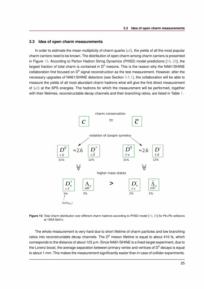
In order to estimate the mean multiplicity of charm quarks ⟨cc⟩, the yields of all the most popularcharm carriers need to be known. The distribution of open charm among charm carriers is presentedin Figure 13. According to Parton Hadron String Dynamics (PHSD) model predictions [19, 20], thelargest fraction of total charm is contained in D0 mesons. This is the reason why the NA61/SHINEcollaboration first focused on D0 signal reconstruction as the test measurement. However, after thenecessary upgrades of NA61/SHINE detectors (see Section 3.5.1), the collaboration will be able tomeasure the yields of all most abundant charm hadrons what will give the first direct measurementof ⟨cc⟩ at the SPS energies. The hadrons for which the measurement will be performed, togetherwith their lifetimes, reconstructable decay channels and their branching ratios, are listed in Table 1.

charm conservation

c = c

violation of izospin symetry

Dc u

0 ≈2.6 Dc d

+ Dc u

0≈2.6 D

c d

-

higher mass states

Dc s

s+ Λ

udcc > D

c ss- Λ

u d cc

≫ ≫

¯

31% 12% 31% 12%

5% 3% 2% 5%

⟨n⟩/⟨nALL⟩

Figure 13: Total charm distribution over different charm hadrons according to PHSD model [19, 20] for Pb+Pb collisionsat 158A GeV/c.

The whole measurement is very hard due to short lifetime of charm particles and low branchingratios into reconstructable decay channels. The D0 meson lifetime is equal to about 410 fs, whichcorresponds to the distance of about 123 µm. Since NA61/SHINE is a fixed-target experiment, due tothe Lorenz boost, the average separation between primary vertex and vertices of D0 decays is equalto about 1 mm. This makes the measurement significantly easier than in case of collider experiments.

25

3.3 Idea of open charm measurements

Table 1: The most frequently produced charm hadrons: their mass, mean lifetime multiplied by the speed of light and thedecay channel (with its branching ratio BR) best suited for measurements are shown. Numerical values are takenfrom Ref. [33].

Hadron Mass [MeV] cτ [µm] Decay channel BR

D0 1864.83 ± 0.05 123 π++K− 3.89%

D+ 1869.65 ± 0.05 312 π++π++K− 9.22%

D+S 1968.34 ± 0.07 150 π++K−+K+ 5.50%

Λc 2286.46 ± 0.14 60 p+π++K− 5.00%

However, additional tracking device (Vertex Detector) is needed to be able to distinguish betweenprimary and the decay vertices of D0 mesons. The schematic idea of D0 measurement is presentedin Figure 14.

Primary beam: ions at 150A GeV/c

Target

SecondaryVertex

PrimaryVertex

𝐾

𝜋

𝜋

𝐾

4.9 cm

Station 2

Station 1

𝐷0

0.1 cm

Figure 14: The schematic picture showing the idea behind D0 meson measurement. Figure from Ref. [24].

26

3.4 NA61/SHINE detector

3.4 NA61/SHINE detector

The NA61/SHINE detector is a multi-purpose spectrometer optimised to study hadron productionin different types of collisions: p+p, h+A (hadron+nucleus), A+A (nucleus+nucleus). The schematicpicture of the detector is presented in Figure 15. The main subdetectors of the whole setup are TimeProjection Chambers. Two of them (Vertex-TPCs, VTPCs) located in the magnetic field togetherwith two large volume Main-TPCs (MTPCs) are main tracking devices. There are also smallerTPCs: GAP-TPC and 3 Forward-TPCs (FTPCs) located along the beam axis. Such a setup givesan excellent capabilities in charged particles momenta measurement and allows for the particleidentification complimented by the information from the Time-of-Flight (ToF) detectors. The lastdetector on the beamline is Projectile Spectator Detector (PSD), which measures the energy ofspectators – non-interaction nucleons. This information is used to determine the centrality in A+Acollisions. Beam particles are measured by an array of beam detectors. They are used for thetrajectory measurement as well as the identification of primary (from SPS) and secondary (fromfragmentation) hadrons and ions. The signal from these detectors is also used for triggering thedata acquisition. In 2016, the whole spectrometer was upgraded by adding Vertex Detector (SAVD)which is described in details in Section 3.4.1.

~13 m

ToF-L

ToF-R

ToF-F

MTPC-R

MTPC-L

VTPC-2VTPC-1

Vertex magnets

Target

GAPTPC

Beam

S4 S5

S2S1

BPD-1 BPD-2 BPD-3

V1 V1V0THCCEDAR

z

x

y

p

SAVD

FTPC-1

FTPC-2/3

PSD

Figure 15: The schematic picture of the NA61/SHINE detector. Figure from Ref. [15].

27

3.4 NA61/SHINE detector

3.4.1 Small-Acceptance Vertex Detector

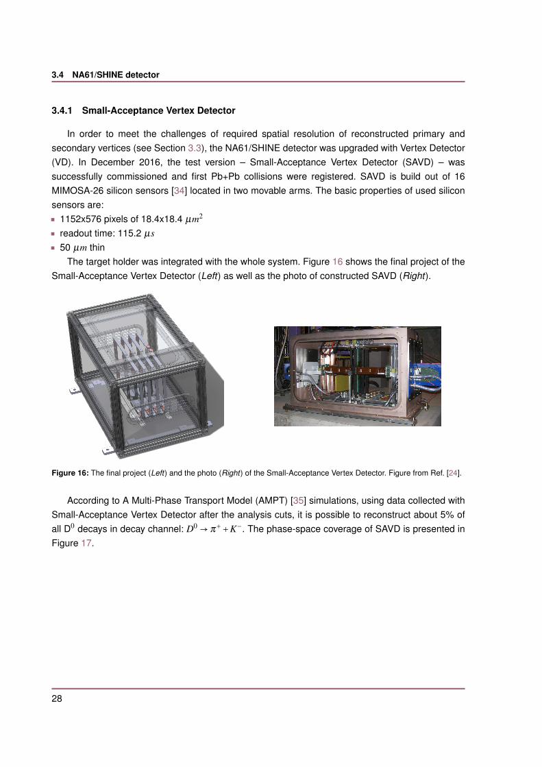
In order to meet the challenges of required spatial resolution of reconstructed primary andsecondary vertices (see Section 3.3), the NA61/SHINE detector was upgraded with Vertex Detector(VD). In December 2016, the test version – Small-Acceptance Vertex Detector (SAVD) – wassuccessfully commissioned and first Pb+Pb collisions were registered. SAVD is build out of 16MIMOSA-26 silicon sensors [34] located in two movable arms. The basic properties of used siliconsensors are:◾ 1152x576 pixels of 18.4x18.4 µm2

◾ readout time: 115.2 µs◾ 50 µm thin

The target holder was integrated with the whole system. Figure 16 shows the final project of theSmall-Acceptance Vertex Detector (Left) as well as the photo of constructed SAVD (Right).

Figure 16: The final project (Left) and the photo (Right) of the Small-Acceptance Vertex Detector. Figure from Ref. [24].

According to A Multi-Phase Transport Model (AMPT) [35] simulations, using data collected withSmall-Acceptance Vertex Detector after the analysis cuts, it is possible to reconstruct about 5% ofall D0 decays in decay channel: D0

→ π++K−. The phase-space coverage of SAVD is presented in

Figure 17.

28

3.5 NA61/SHINE beyond 2020

Figure 17: Transverse momentum (momentum in plane perpendicular to beam axis) and rapidity (y = 12 ln E+pL

E−pL, where: E

– energy, pL = pz – momentum along z axis; yCM – rapidity calculated in center-of-mass frame) distributions

of D0 + D0 mesons produced in central Pb+Pb collisions at 150A GeV/c simulated within the AMPT model

and corresponding to 3 ⋅106 events. Left : Results for all produced D0 + D0 mesons. Right : results for D0 + D0

mesons fulfilling the following criteria: decay D0→ π

++K− and D0 → π

−+K+, both decay products registered

by the SAVD, passing background suppression and quality cuts [36]. Figure from Ref. [24].

3.5 NA61/SHINE beyond 2020

Although the feasibility studies on charm were already performed, the precise measurementsof charm hadrons production at the SPS energies are expected to be done in 2022-2024. For thispurpose, during the Long Shutdown 2 at CERN (2019-2020), the NA61/SHINE detector will besignificantly upgraded [24]. The plans of the upgrade are presented in Section 3.5.1. From the pointof view of charm physics programme, the most important upgrade concerns the NA61/SHINE VertexDetector. This upgrade is discussed in Section 3.5.2.

3.5.1 NA61/SHINE detector upgrades

During the Long Shutdown 2 at CERN (2019-2020), the NA61/SHINE spectrometer is plannedto be upgraded [24]. Most of the upgrades are dedicated to the charm physics programme whichrequires the increase of the phase-space coverage of Vertex Detector and the tenfold increase ofdata taking rate to about 1 kHz. To obtain the required goals, the following is planned to be done:◾ construction of new NA61/SHINE Vertex Detector,◾ replacement of TPC read-out electronics,◾ preparing new data acquisition and trigger system,◾ update of Projectile Spectator Detector.Additionally, new Time-of-Flight detectors will be constructed to improve the particle identification inmid-rapidity (central region of rapidity).The overall picture of all upgrades is presented in Figure 18.

29

3.5 NA61/SHINE beyond 2020

Figure 18: Summary picture of all upgrade plans of the NA61/SHINE detector. Figure from Ref. [24].

3.5.2 NA61/SHINE Vertex Detector

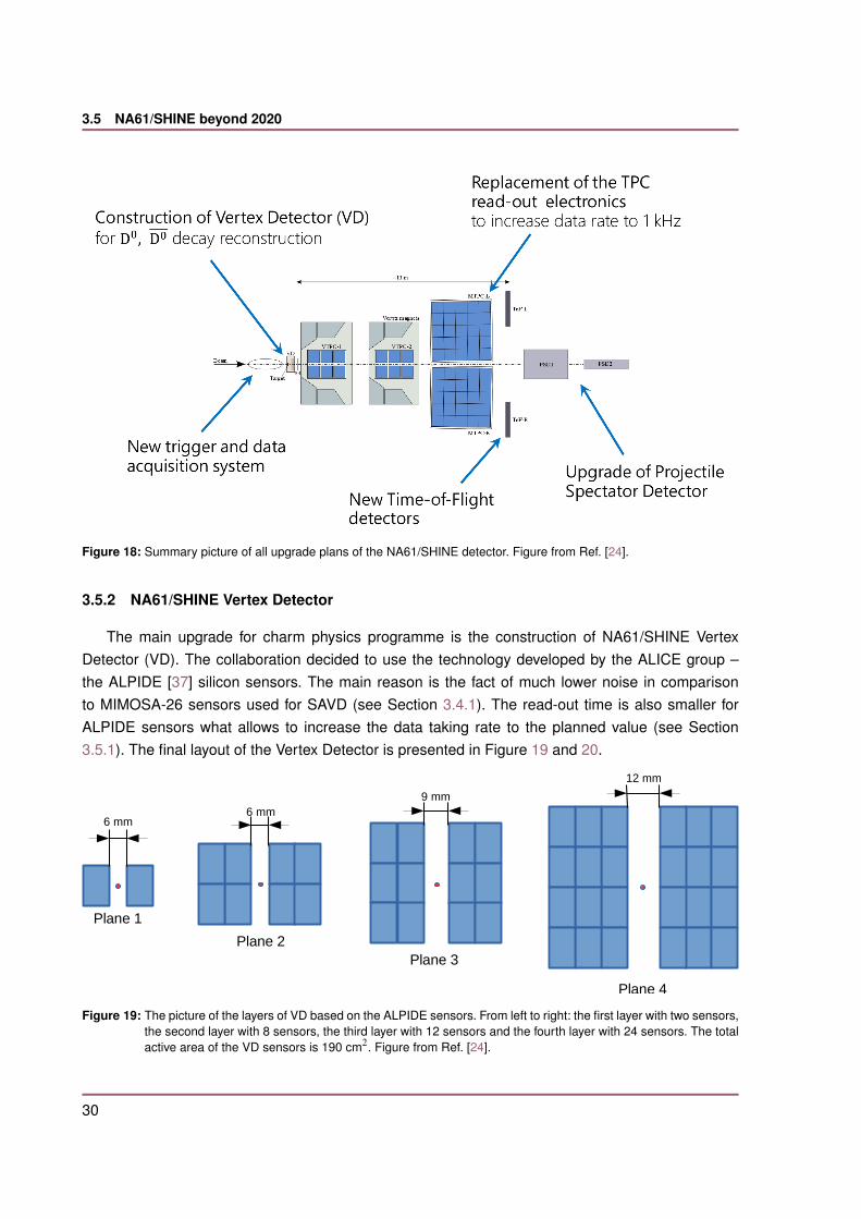
The main upgrade for charm physics programme is the construction of NA61/SHINE VertexDetector (VD). The collaboration decided to use the technology developed by the ALICE group –the ALPIDE [37] silicon sensors. The main reason is the fact of much lower noise in comparisonto MIMOSA-26 sensors used for SAVD (see Section 3.4.1). The read-out time is also smaller forALPIDE sensors what allows to increase the data taking rate to the planned value (see Section3.5.1). The final layout of the Vertex Detector is presented in Figure 19 and 20.

Plane 1

Plane 2Plane 3

Plane 4

6 mm6 mm

9 mm

12 mm

Figure 19: The picture of the layers of VD based on the ALPIDE sensors. From left to right: the first layer with two sensors,the second layer with 8 sensors, the third layer with 12 sensors and the fourth layer with 24 sensors. The totalactive area of the VD sensors is 190 cm2. Figure from Ref. [24].

30

3.5 NA61/SHINE beyond 2020

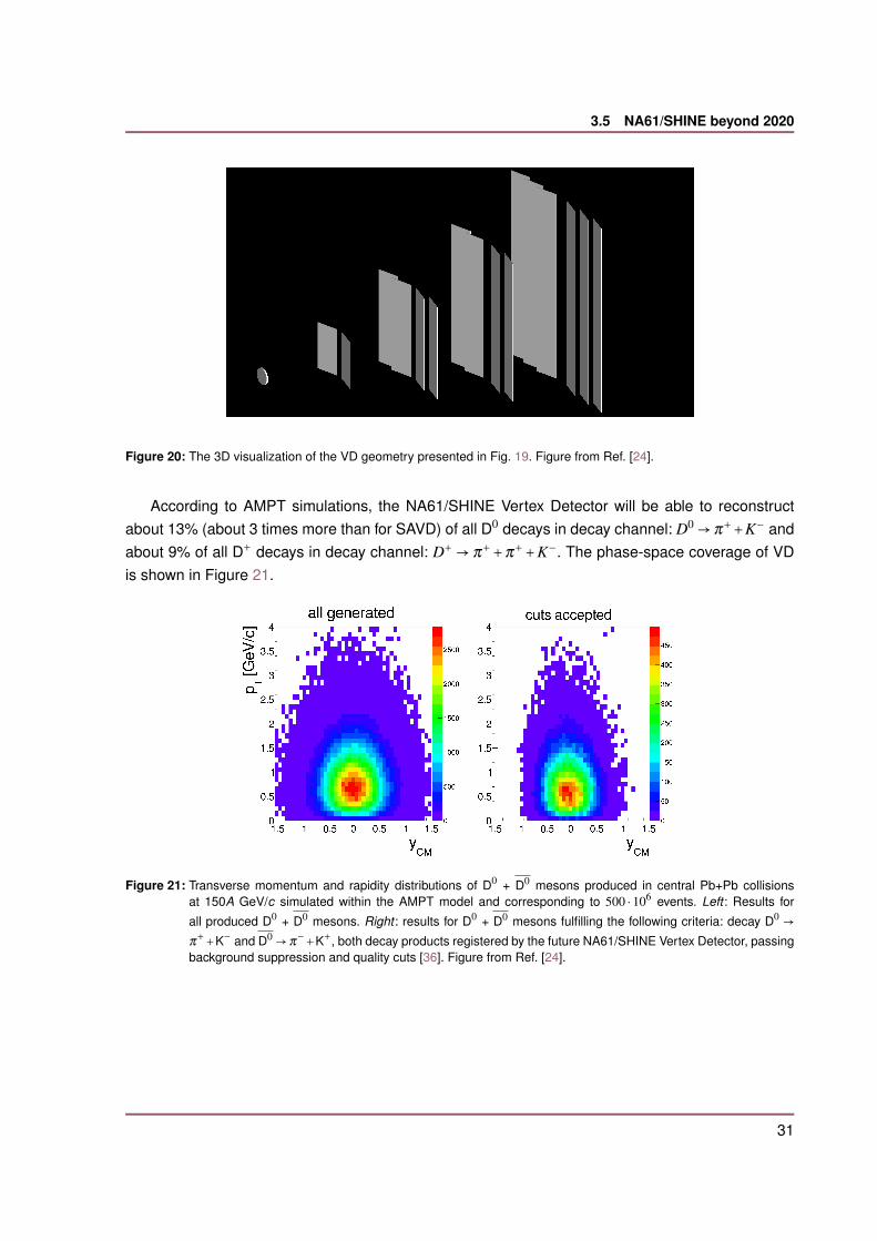
Figure 20: The 3D visualization of the VD geometry presented in Fig. 19. Figure from Ref. [24].

According to AMPT simulations, the NA61/SHINE Vertex Detector will be able to reconstructabout 13% (about 3 times more than for SAVD) of all D0 decays in decay channel: D0

→ π++K− and

about 9% of all D+ decays in decay channel: D+ → π++π++K−. The phase-space coverage of VD

is shown in Figure 21.

Figure 21: Transverse momentum and rapidity distributions of D0 + D0 mesons produced in central Pb+Pb collisionsat 150A GeV/c simulated within the AMPT model and corresponding to 500 ⋅ 106 events. Left : Results for

all produced D0 + D0 mesons. Right : results for D0 + D0 mesons fulfilling the following criteria: decay D0→

π++K− and D0→ π

−+K+, both decay products registered by the future NA61/SHINE Vertex Detector, passing

background suppression and quality cuts [36]. Figure from Ref. [24].

31

4. Data reconstruction

This thesis has a significant input to the reconstruction chain used for the data collected bySmall-Acceptance Vertex Detector (see Section 3.4.1). The whole data reconstruction includes thefollowing steps:◾ geometry tuning,◾ track finding,◾ primary vertex reconstruction,◾ SAVD-TPC track matching,As a part of this thesis the algorithms for geometry tuning and VD-TPC track matching wereimplemented. These algorithms are described in Sections 4.1 and 4.2, respectively. Both algorithmswere tested on Pb+Pb collisions at 150A GeV/c registered in December 2016 using SAVD, howeverthey can be easily adapted for the future measurements which will be done using upgradedNA61/SHINE Vertex Detector (see Section 3.5.2). The track finding was performed using thecombinatorial method by checking the colinearity of all possible combinations of clusters fromdifferent stations. Primary vertex was reconstructed by averaging the positions of the pointscorresponding to the Distance of Closest Approach (DCA – the smallest distance) between pairsof tracks.

4.1 Vertex Detector alignment

In order to optimise the spatial resolution of registered particles hits, the position of all sensorshas to be known with very high precision. It would be impossible to measure the position of allsensors precisely enough before every data taking period. Even after opening and closing the armsof VD for beam tuning, the geometry is slightly changed. Thus, the only reasonable solution wasto prepare the algorithm which calculates the required geometry corrections and apply them forthe collected data. For this purpose the data registered without the magnetic field were used. Evenbefore the geometry tuning it was possible to reconstruct the tracks candidates, but the efficiencywas very poor. Such a reconstructed tracks candidates were used for the silicon sensors alignment.For the proper geometry, hits produced by one particle, should lie on the same straight line. In orderto estimate the collinearity of 3 hits the ”dev” variable was introduced:

devx =x1+x3

2−x2 (3)

devy =y1+y3

2−y2 (4)

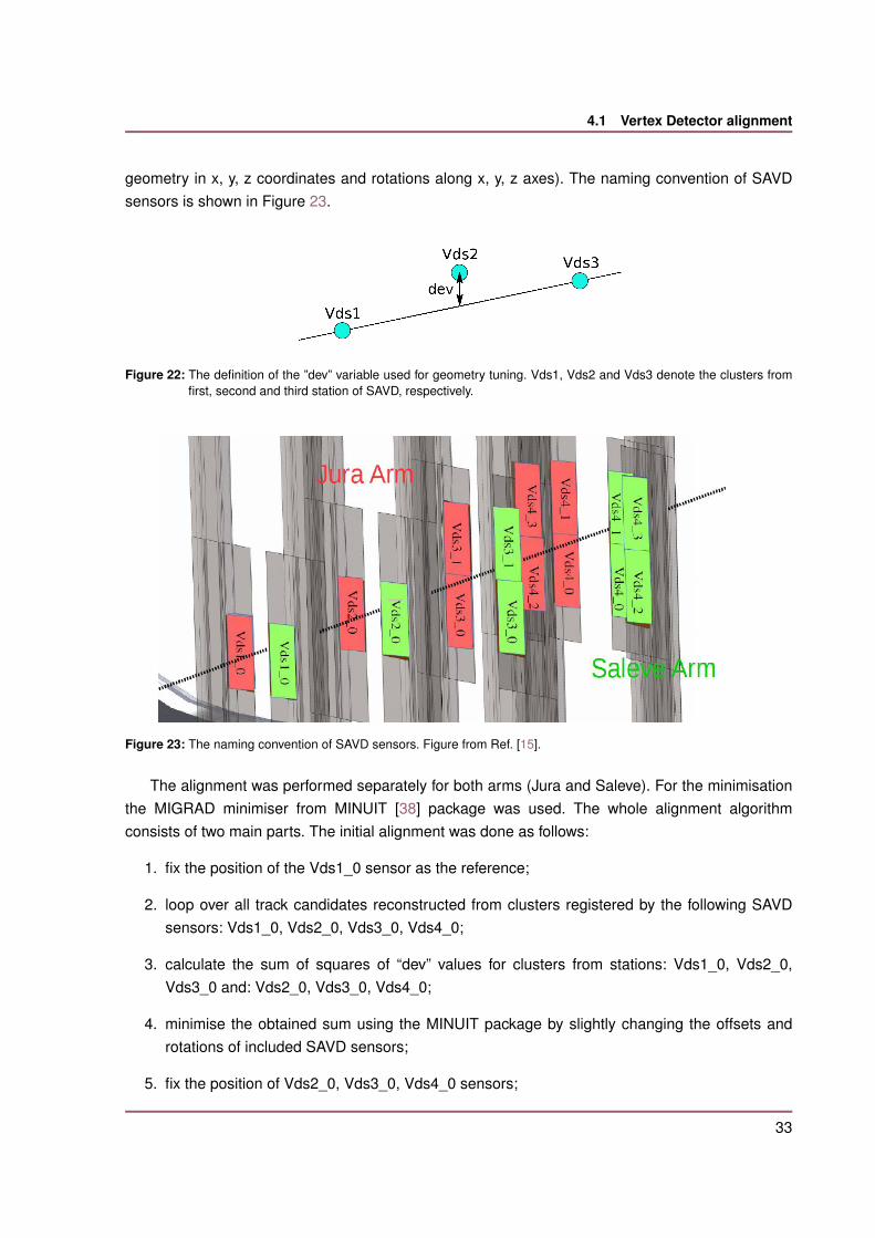
where x1, x2, x3 and y1, y2, y3 correspond to the cluster x and y position on the first, second and thirdstation accordingly. The meaning of ”dev” variable is presented in Figure 22. For proper geometry,the distribution of ”dev” for reconstructed tracks should present a narrow peak centered at zero.Thus, the algorithm of alignment should find a minimal value of the sum of squares of ”dev” valuesby changing the position of sensors (each sensor has 6 degrees of freedom: offsets from the nominal

32

4.1 Vertex Detector alignment

geometry in x, y, z coordinates and rotations along x, y, z axes). The naming convention of SAVDsensors is shown in Figure 23.

Figure 22: The definition of the ”dev” variable used for geometry tuning. Vds1, Vds2 and Vds3 denote the clusters fromfirst, second and third station of SAVD, respectively.

Figure 23: The naming convention of SAVD sensors. Figure from Ref. [15].

The alignment was performed separately for both arms (Jura and Saleve). For the minimisationthe MIGRAD minimiser from MINUIT [38] package was used. The whole alignment algorithmconsists of two main parts. The initial alignment was done as follows:

1. fix the position of the Vds1_0 sensor as the reference;

2. loop over all track candidates reconstructed from clusters registered by the following SAVDsensors: Vds1_0, Vds2_0, Vds3_0, Vds4_0;

3. calculate the sum of squares of “dev” values for clusters from stations: Vds1_0, Vds2_0,Vds3_0 and: Vds2_0, Vds3_0, Vds4_0;

4. minimise the obtained sum using the MINUIT package by slightly changing the offsets androtations of included SAVD sensors;

5. fix the position of Vds2_0, Vds3_0, Vds4_0 sensors;

33

4.1 Vertex Detector alignment

6. do the same minimisation for track candidates reconstructed from clusters registered by thefollowing SAVD sensors: Vds1_0, Vds2_0, Vds3_1, Vds4_1;

7. fix the position of Vds3_1, Vds4_1;

8. do the analogous minimisation for track candidates reconstructed from clusters from SAVDsensors: Vds1_0, Vds2_0, Vds3_0, Vds4_2 and fix the position of the Vds4_2 sensor;

9. do the analogous minimisation for track candidates reconstructed from clusters from SAVDsensors: Vds1_0, Vds2_0, Vds3_1, Vds4_3 and fix the position of the Vds4_3 sensor.

The final alignment was done for all sensors simultaneously. Instead of ”dev” variable, thedistributions of residuals between fitted tracks and clusters were used. This part consists of thefollowing steps:

1. loop over all track candidates and create the distributions of residuals between refitted tracksand clusters;

2. minimize the sum of estimators of mean and standard deviation values for all the createddistributions using the MINUIT package by changing the offsets and rotations of SAVDsensors.

In order to estimate the improvement of the spatial clusters resolution after geometry tuning, thedistributions of residuals between fitted tracks and clusters for all the sensors (newGeometry )were compared with the same distributions obtained before the geometry tuning (oldGeometry ).The Pb+Pb collisions at 150A GeV/c registered in December 2016 were analysed. The Gaussianfunctions were fitted to all the distributions and the standard deviation (σ ) values were used tocalculate the improvement factor from the following formula:

improvement =σoldGeometry−σnewGeometry

σoldGeometry⋅100% (5)

The sigma value (σ ) corresponds to the spatial resolution of clusters position, so the improvementfactor shows improvement of spatial clusters resolution after final geometry tuning. The averagevalues of improvement factors for both arms are shown in Table 2. The example comparison of thedistributions of residuals for data before and after geometry tuning is presented in Figure 24.

Sensors used for track reconstructionImprovement FactorSaleve Jura

Vds1_0, Vds2_0, Vds3_0, Vds4_0 20.23% 19.31%Vds1_0, Vds2_0, Vds3_1, Vds4_1 20.24% 13.05%Vds1_0, Vds2_0, Vds3_0, Vds4_2 1.07% –Vds1_0, Vds2_0, Vds3_1, Vds4_3 19.77% 3.82%

Table 2: Average values of improvement factors calculated from Formula (5). The Vds4_2 sensor from Jura arm was notworking properly and that is why there were no tracks reconstructed using this sensor.

34

4.1 Vertex Detector alignment

resX_Vds2_down1 [mm]0.02− 0.015− 0.01− 0.005− 0 0.005 0.01 0.015 0.02

coun

ts

0

50

100

150

200

250

300

350

400

450

500

before geometry tuningafter geometry tuning

resY_Vds4_down1 [mm]0.03− 0.02− 0.01− 0 0.01 0.02 0.03

coun

ts

0

50

100

150

200

250before geometry tuningafter geometry tuning

Figure 24: Left : The distribution of x residuals between fitted tracks and hits registered by the Vds2_0 sensor in theJura arm. The improvement factor, calculated from Formula (5), is 20%. Right : The distribution of y residualsbetween fitted tracks and hits registered by the Vds4_0 sensor in the Saleve arm. The improvement factor,calculated from Formula (5), is 22%. Distributions before and after final geometry tuning are shown by blueand red histograms, respectively.

4.1.1 Example results

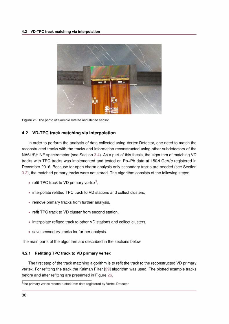
Some of the geometry corrections, calculated in the way described in Section 4.1, hadunexpectedly big values. The example results for one of the sensors from Jura fourth station arelisted below:◾ rotations along x, y, z axes:◻ rotX = -0.01 (0.6o)◻ rotY = 0.01 (0.6o)◻ rotZ = -0.049 (2.8o)

◾ offsets from nominal geometry in x, y, z:◻ offsetX = 2.1 mm◻ offsetY = 1.1 mm◻ offsetZ = 0.5 mm

The photo of this sensor is presented in Figure 25. After opening SAVD for some service work, itturned out that the sensors were indeed shifted and rotated by such big values. It was caused bya problem with phase changing material (with changing temperature) which was used to glue thesensors to the ladders. This result confirms the validity of the implemented alignment algorithm.

35

4.2 VD-TPC track matching via interpolation

Figure 25: The photo of example rotated and shifted sensor.

4.2 VD-TPC track matching via interpolation

In order to perform the analysis of data collected using Vertex Detector, one need to match thereconstructed tracks with the tracks and information reconstructed using other subdetectors of theNA61/SHINE spectrometer (see Section 3.4). As a part of this thesis, the algorithm of matching VDtracks with TPC tracks was implemented and tested on Pb+Pb data at 150A GeV/c registered inDecember 2016. Because for open charm analysis only secondary tracks are needed (see Section3.3), the matched primary tracks were not stored. The algorithm consists of the following steps:

◾ refit TPC track to VD primary vertex3,

◾ interpolate refitted TPC track to VD stations and collect clusters,

◾ remove primary tracks from further analysis,

◾ refit TPC track to VD cluster from second station,

◾ interpolate refitted track to other VD stations and collect clusters,

◾ save secondary tracks for further analysis.

The main parts of the algorithm are described in the sections below.

4.2.1 Refitting TPC track to VD primary vertex

The first step of the track matching algorithm is to refit the track to the reconstructed VD primaryvertex. For refitting the track the Kalman Filter [39] algorithm was used. The plotted example tracksbefore and after refitting are presented in Figure 26.

3the primary vertex reconstructed from data registered by Vertex Detector

36

4.2 VD-TPC track matching via interpolation

z [cm]650− 600− 550− 500− 450− 400− 350−

x [c

m]

5−

0

5

10

15

20

25

30

VD primary vertexTPC clusterstrack

z [cm]650− 600− 550− 500− 450− 400− 350−

x [c

m]

5−

0

5

10

15

20

25

30

VD primary vertexTPC clusterstrack

Figure 26: Left : Track before refitting to VD primary vertex. The vertexing precision (the uncertainty of reconstructedvertices position) from TPC reconstruction is on the order of cm. Right : Track after refitting to VD primaryvertex. On both plots the coordinates system is as introduced in Figure 15.

4.2.2 Track interpolation to VD stations and cluster collection

As the second step, the tracks refitted to VD primary vertex were interpolated to all VD stationsin order to collect the matching clusters. For every station the distribution of the distances betweeninterpolated tracks and all VD clusters were created. The comparison of such a distribution for tracksbefore (left) and after (right) refitting to VD primary vertex is presented in Figure 27. The right pictureshows huge combinatorial background with the correlation peak from matched tracks and clusters.For each sensor, the correlation peak was fitted with Gaussian function and the standard deviationvalue (σ ) was used for the matching cut for primary tracks. If the distance between interpolated trackand cluster is smaller than 2σ , the cluster is accepted as matched. The 2σ cut was used in order tomake sure that only primary tracks were matched in this step. Finally, the track was accepted as theprimary track if at least one VD cluster was matched. The example of primary track is illustrated inFigure 28.

37

4.2 VD-TPC track matching via interpolation

Y_VDclusters - Y_interpolatedTrack [cm]0.4− 0.3− 0.2− 0.1− 0 0.1 0.2 0.3 0.4

coun

ts

22000

24000

26000

28000

30000

32000

Y_VDclusters - Y_interpolatedTrack [cm]0.4− 0.3− 0.2− 0.1− 0 0.1 0.2 0.3 0.4

coun

ts

16000

18000

20000

22000

24000

Figure 27: The distributions of the distances between interpolated tracks and all VD clusters from first station before (Left)and after (Right) refitting to VD primary vertex. It shows that in order to see the correlation between matchingtracks and clusters, the first step of the algorithm (see Section 4.2.1) is needed.

z [cm]650− 600− 550− 500− 450− 400− 350−

x [c

m]

5−

0

5

10

15

20

25

30

VD primary vertexVD clustersTPC clusterstrack

Figure 28: The matched VD clusters to TPC track.

4.2.3 Refitting TPC track to VD clusters

After removing the primary tracks, the matching algorithm for secondary tracks was performed.In the first step, each track is combined with all VD clusters from the second station. The exampletrack before and after refitting is illustrated in Figure 29.

38

4.2 VD-TPC track matching via interpolation

z [cm]650− 600− 550− 500− 450− 400− 350−

x [c

m]

10−

5−

0

5

10

15

20

VD primary vertexVD cluster from 2nd stationTPC clusterstrack

z [cm]650− 600− 550− 500− 450− 400− 350−

x [c

m]

10−

5−

0

5

10

15

20

VD primary vertexVD cluster from 2nd stationTPC clusterstrack

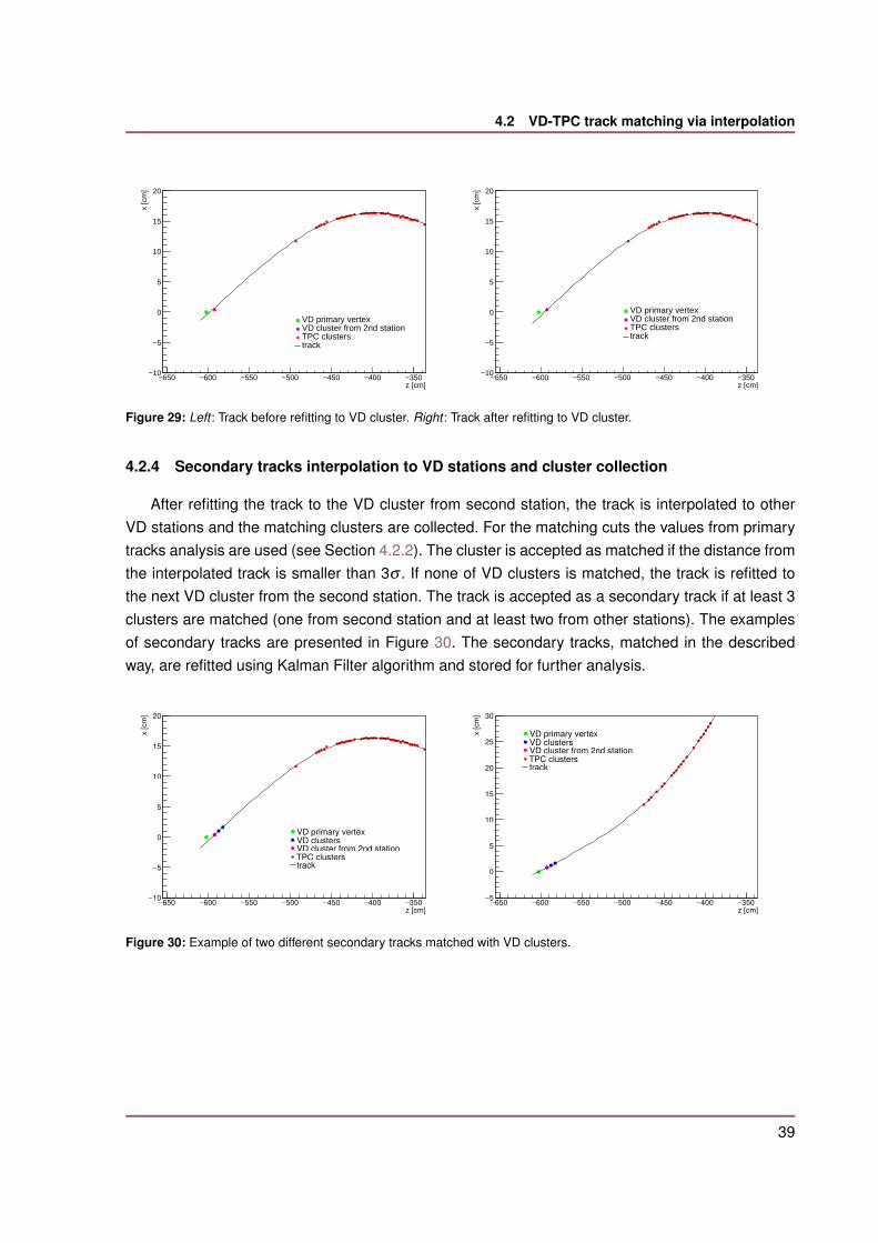
Figure 29: Left : Track before refitting to VD cluster. Right : Track after refitting to VD cluster.

4.2.4 Secondary tracks interpolation to VD stations and cluster collection

After refitting the track to the VD cluster from second station, the track is interpolated to otherVD stations and the matching clusters are collected. For the matching cuts the values from primarytracks analysis are used (see Section 4.2.2). The cluster is accepted as matched if the distance fromthe interpolated track is smaller than 3σ . If none of VD clusters is matched, the track is refitted tothe next VD cluster from the second station. The track is accepted as a secondary track if at least 3clusters are matched (one from second station and at least two from other stations). The examplesof secondary tracks are presented in Figure 30. The secondary tracks, matched in the describedway, are refitted using Kalman Filter algorithm and stored for further analysis.

z [cm]650− 600− 550− 500− 450− 400− 350−

x [c

m]

10−

5−

0

5

10

15

20

VD primary vertexVD clustersVD cluster from 2nd stationTPC clusterstrack

z [cm]650− 600− 550− 500− 450− 400− 350−

x [c

m]

5−

0

5

10

15

20

25

30

VD primary vertexVD clustersVD cluster from 2nd stationTPC clusterstrack

Figure 30: Example of two different secondary tracks matched with VD clusters.

39

5. Data analysis

In order to test the implemented reconstruction algorithms (see Section 4) the analysis of K0s

signal was performed. It is described in details in Section 5.1. Section 5.2 presents the D0+D0 signalreconstruction which is the most important result of this thesis. Both analyses were performed onPb+Pb collisions at 150A GeV/c registered in December 2016.

5.1 K0s test signal

The most popular decay channel of K0s

4 particles is the decay into two pions (K0s → π

++π−) with

the branching ratio of 69,2%. Thus, in order to reconstruct the K0s signal, all the secondary tracks

reconstructed as described in Section 4.2.3 and 4.2.4 were grouped into pairs. For each pair theinvariant mass of parent particle was calculated assuming the pion mass of both daughter particlesand put into the histogram. The invariant mass was calculated from the following formula:

Minv =√

(E1+E2)2−(p1+p2)2 (6)

where: Minv – invariant mass, E1, E2 – energy of first and second particle, p1, p2 – momentum of firstand second particle. The secondary vertex was calculated as the point of closest approach betweentracks. In order to reduce the combinatorial background, the cuts on the following variables wereapplied:◾ longitudinal position of the track pair vertex relative to primary vertex: Vz > 0 µm,◾ parent particle impact parameter (the distance between mother particle track and primary vertex):

D < 400 µmThe value of second cut was based on D0 analysis (see Section 5.2.1). The example distribution (forabout 140k events) of reconstructed invariant mass with K0

s peak is presented in Figure 31.

]2[GeV/cππM0.47 0.48 0.49 0.5 0.51 0.52 0.53

coun

ts

80

100

120

140

160

180

200

220

240

σK0s=1.25 ± 0.44 MeVyield= 85

Figure 31: The reconstructed signal of K0s particle. The black line corresponds to the K0

s mass taken from Ref. [33].

4Quark content: ds+sd√2

, mass: 497.611±0.013 MeV, lifetime: (0.8954±0.0004) ⋅10−10 s [33]

40

5.1 K0s test signal

From the data analysis it was observed, that the whole statistics can be divided into two samples:◾ sample 1 (runs: 27256 - 27355) – with poor quality of K0

s signal,◾ sample 2 (runs: 27384 - 27452) – with good quality of K0

s signal.For data from sample 1 the signal can be visible only for the collisions which were taken at the endof this sample data taking. The comparison of results from both samples is presented in Figure 32.One can observe that the signals from different samples are not centered at the same mass. Thisshift is caused by the lack of final calibration of the data. It was found that between the registrationof the data from both samples, there was a ten-hours break in the data taking. From this fact, onemay conclude that something was changing in time during the data taking and was not correctedyet. This is why for the final analysis of D0 signal only collisions from the second sample were used(about 140k events).

]2 [GeV/cππM0.47 0.48 0.49 0.5 0.51 0.52 0.53

coun

ts

0

2

4

6

8

10

12

14

16

18

20

22

24

]2 [GeV/cππM0.47 0.48 0.49 0.5 0.51 0.52 0.53

coun

ts

80

100

120

140

160

180

200

220

240

]2[GeV/cππM0.48 0.485 0.49 0.495 0.5 0.505 0.51 0.515 0.52

coun

ts

100

120

140

160

180

200

220

240

0.485 0.49 0.495 0.5 0.505 0.51 0.515

first sample

second sample

Figure 32: Top Left : K0s signal obtained from first sample. Top Right : K0

s signal obtained from second sample. Bottom:The comparison of K0

s signal obtained from different samples of data. Data from first sample were scaled byeye. The black line corresponds to the K0

s mass taken from Ref. [33].

41

5.2 D0 signal

5.2 D0 signal

The idea of D0 measurement is described in Section 3.3. The analysis was performed usingthe Pb+Pb data at 150A GeV/c registered in December 2016, reconstructed using the algorithmsdiscussed in Section 4. In order to reduce the background the track cuts described in Section 5.2.1were applied. The final result is presented in Section 5.2.2.

5.2.1 Track cuts

The cut values were taken from Ref. [40]. These cuts are based on the simulation and are chosento maximise the signal to noise ratio (SNR) for reconstructed D0 peak. The values are presented inFigure 33 by the dashed vertical lines, together with the distributions of the variables for which thecuts were applied:◾ pT – transverse momentum – the momentum of daughter particle in the plane perpendicular to

the beam axis,◾ d – daughter particle impact parameter – the distance between the track and primary vertex,◾ Vz – longitudinal position of the track pair vertex relative to primary vertex,◾ dp – mother particle impact parameter.For experimental data the procedure of choosing the cut values is not finished yet. Thecorresponding distributions for experimental data are shown in Figure 34. Comparing the plots tothe distributions presented in Figure 33, one may see that most of the primary tracks were removedfrom the analysis by the reconstruction algorithm (see Section 4). There are less tracks with smallvalues of particle impact parameter (d). Also the peak in Vz distribution, which comes from primarytracks is significantly smaller. Based on presented plots, different cut values close to the values fromsimulation were tested and final cuts were selected as follows:◾ transverse momentum: pT > 0.42 GeV/c,◾ track impact parameter: d > 42 µm,◾ longitudinal position of the secondary vertex (reconstructed from track pair) relative to primary

vertex: Vz > 450 µm,◾ parent particle impact parameter: dp < 400 µm.

42

5.2 D0 signal

Figure 33: The distribution of the cuts variables from the simulation (AMPT model, Pb+Pb at 150A GeV/c) for D0+D0

signal (red) and background (blue). The background distributions were obtained using all the tracks (primaryand secondary). Figure from Ref. [40].

[GeV/c]T

p0 0.5 1 1.5 2 2.5 3 3.5

coun

ts

1

10

210

310

410

510

610

710

[cm]d0 0.01 0.02 0.03 0.04 0.05 0.06 0.07

coun

ts

1

10

210

310

410

510

610

710

[cm]ZV0.6− 0.4− 0.2− 0 0.2 0.4 0.6 0.8

coun

ts

1

10

210

310

410

510

[cm]Pd0 0.01 0.02 0.03 0.04 0.05 0.06 0.07 0.08

coun

ts

1

10

210

310

410

510

Figure 34: The distribution of the cuts variables from the reconstructed data.

43

5.2 D0 signal

5.2.2 Invariant mass distributions

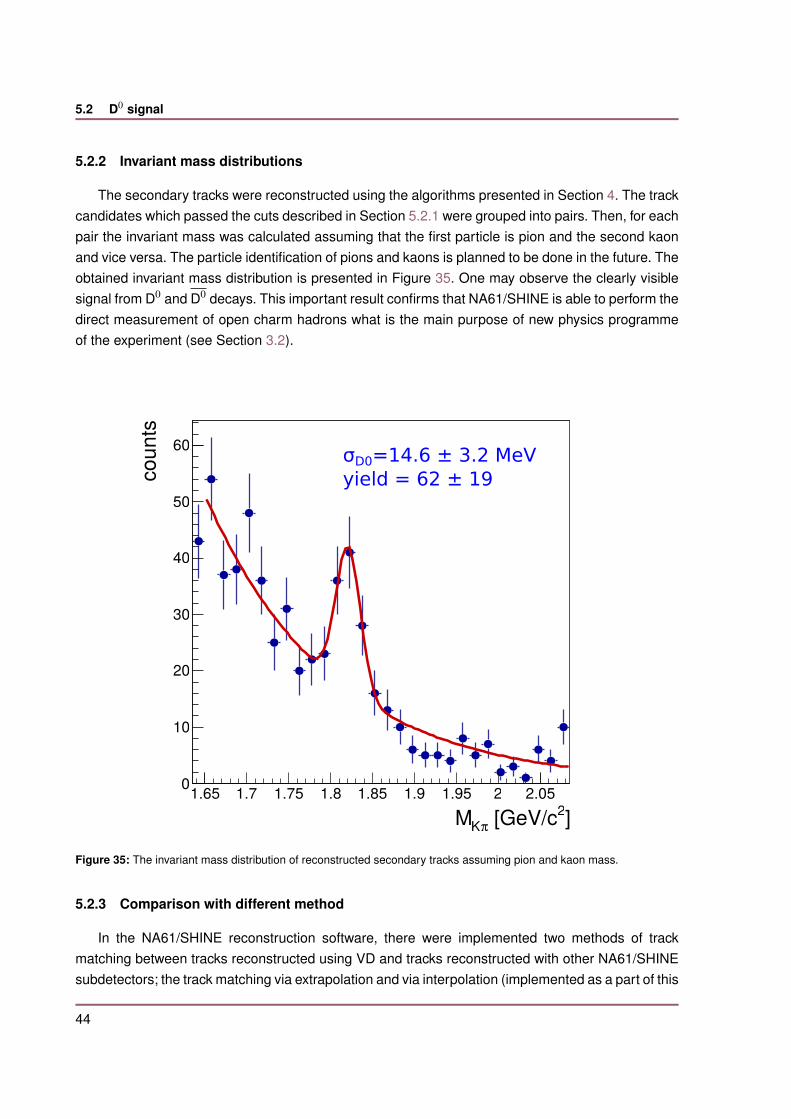
The secondary tracks were reconstructed using the algorithms presented in Section 4. The trackcandidates which passed the cuts described in Section 5.2.1 were grouped into pairs. Then, for eachpair the invariant mass was calculated assuming that the first particle is pion and the second kaonand vice versa. The particle identification of pions and kaons is planned to be done in the future. Theobtained invariant mass distribution is presented in Figure 35. One may observe the clearly visiblesignal from D0 and D0 decays. This important result confirms that NA61/SHINE is able to perform thedirect measurement of open charm hadrons what is the main purpose of new physics programmeof the experiment (see Section 3.2).

]2[GeV/cπKM1.65 1.7 1.75 1.8 1.85 1.9 1.95 2 2.05

coun

ts

0

10

20

30

40

50

60σD0=14.6 ± 3.2 MeVyield = 62 ± 19

Figure 35: The invariant mass distribution of reconstructed secondary tracks assuming pion and kaon mass.

5.2.3 Comparison with different method

In the NA61/SHINE reconstruction software, there were implemented two methods of trackmatching between tracks reconstructed using VD and tracks reconstructed with other NA61/SHINEsubdetectors; the track matching via extrapolation and via interpolation (implemented as a part of this

44

5.2 D0 signal

thesis, see Section 4.2). In the first method, the VD and TPC tracks were extrapolated to the commonplane (VTPC-1 front surface) and the matching tracks were found [40]. Using this method also D0

and D0 signal was observed. The comparison of the final signal obtained from both methods ispresented in Figure 36. Comparing these methods, one may conclude that the interpolation methodnot only confirmed the obtained D0 and D0 signal, but also improved the signal resolution by a factorof about 3.

]2[GeV/cπKM1.65 1.7 1.75 1.8 1.85 1.9 1.95 2 2.05

coun

ts

0

10

20

30

40

50

60σD0=14.6 ± 3.2 MeVyield = 62 ± 19

Figure 36: The invariant mass distribution of reconstructed secondary tracks assuming pion and kaon mass obtainedfrom track matching via extrapolation [40] (Left) and via interpolation (Right).

45

6. Conclusions

This thesis has a significant input to the feasibility studies of new physics programme of theNA61/SHINE experiment. The programme is motivated by three main questions:◾ What is the mechanism of open charm production?◾ How does the onset of deconfinement impact open charm production?◾ How does the formation of quark-gluon plasma impact J/ψ production?In order to answer these questions, the knowledge of mean multiplicity of charm quark pairs ⟨cc⟩produced in a full phase space in heavy-ion collisions is needed. The measurement of the mostpopular charm mesons (D0, D0, D+, D−) is enough to estimate the mean multiplicity of charmquark pairs. However, due to very short lifetime of these mesons, their measurement requiresa micro vertex detector. In December 2016, the NA61/SHINE spectrometer was upgraded by aSmall-Acceptance version of Vertex Detector and first pilot data for Pb+Pb collisions at 150A GeV/cwere registered.

The first part of the work described in this thesis was to implement two algorithms used indata reconstruction. The first was the algorithm of the silicon sensors alignment. For this purposethe data taken without magnetic field were used. The geometry corrections were found by theminimisation of the distances between fitted track and collected clusters. The final results improvedthe clusters spatial resolution up to 20%. The second algorithm was the track matching betweendata reconstructed with SAVD and data from other subdetectors. The algorithm of matching viainterpolation was used. At first, tracks are refitted to VD primary vertex (for primary tracks) or VDclusters from defined station (for secondary tracks) and then interpolated to other VD stations andthe matching clusters are collected. Finally, the whole track is refitted using Kalman Filter.

After the data reconstruction, the analysis of K0s signal was performed to test the implemented

algorithms. The signal was successfully observed. The analysis also showed the problem with datacalibration, thus only the second half of collected statistics, which gave better results, was used forthe final analysis.

The main aim of this work was to observe the first indication of D0 and D0 signal in collisionsof nuclei at the SPS energies. The proper analysis was performed and the distribution of invariantmass of pairs of reconstructed secondary tracks was calculated. The final result shows the clearlyvisible signal of D0 and D0 decays. It is the first direct measurement of open charm hadrons inheavy-ion collisions at the SPS energies. However, the statistics is not enough to make some firstconclusions on the charm production cross-section. The performed test measurement confirms, thatusing the new Vertex Detector, the NA61/SHINE experiment is able to reconstruct the signal fromopen charm hadrons decays and thus to perform high statistics studies on open charm productionin heavy-ion collisions. The implemented algorithms and data analysis software will be also used forhigh statistics data which will be collected in the future.

47

BIBLIOGRAPHY

Bibliography

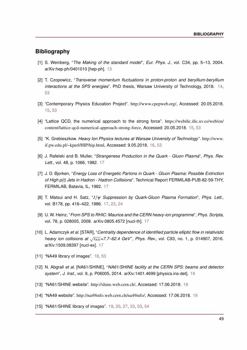
[1] S. Weinberg, “The Making of the standard model”, Eur. Phys. J., vol. C34, pp. 5–13, 2004.arXiv:hep-ph/0401010 [hep-ph]. 13

[2] T. Czopowicz, “Transverse momentum fluctuations in proton-proton and beryllium-berylliuminteractions at the SPS energies”. PhD thesis, Warsaw University of Technology, 2018. 14,53

[3] “Contemporary Physics Education Project”. http://www.cpepweb.org/, Accessed: 20.05.2018.15, 53

[4] “Lattice QCD, the numerical approach to the strong force”. https://webific.ific.uv.es/web/en/content/lattice-qcd-numerical-approach-strong-force, Accessed: 20.05.2018. 15, 53

[5] “K. Grebieszkow. Heavy Ion Physics lectures at Warsaw University of Technology ”. http://www.if.pw.edu.pl/~kperl/HIP/hip.html, Accessed: 9.05.2018. 16, 53

[6] J. Rafelski and B. Muller, “Strangeness Production in the Quark - Gluon Plasma”, Phys. Rev.Lett., vol. 48, p. 1066, 1982. 17

[7] J. D. Bjorken, “Energy Loss of Energetic Partons in Quark - Gluon Plasma: Possible Extinctionof High p(t) Jets in Hadron - Hadron Collisions”. Technical Report FERMILAB-PUB-82-59-THY,FERMILAB, Batavia, IL, 1982. 17

[8] T. Matsui and H. Satz, “J/ψ Suppression by Quark-Gluon Plasma Formation”, Phys. Lett.,vol. B178, pp. 416–422, 1986. 17, 23, 24

[9] U. W. Heinz, “From SPS to RHIC: Maurice and the CERN heavy-ion programme”, Phys. Scripta,vol. 78, p. 028005, 2008. arXiv:0805.4572 [nucl-th]. 17

[10] L. Adamczyk et al. [STAR], “Centrality dependence of identified particle elliptic flow in relativisticheavy ion collisions at

√sNN=7.7–62.4 GeV ”, Phys. Rev., vol. C93, no. 1, p. 014907, 2016.

arXiv:1509.08397 [nucl-ex]. 17

[11] “NA49 library of images”. 18, 53

[12] N. Abgrall et al. [NA61/SHINE], “NA61/SHINE facility at the CERN SPS: beams and detectorsystem”, J. Inst., vol. 9, p. P06005, 2014. arXiv:1401.4699 [physics.ins-det]. 19

[13] “NA61/SHINE website”. http://shine.web.cern.ch/, Accessed: 17.06.2018. 19

[14] “NA49 website”. http://na49info.web.cern.ch/na49info/, Accessed: 17.06.2018. 19

[15] “NA61/SHINE library of images”. 19, 20, 27, 33, 53, 54

49

BIBLIOGRAPHY

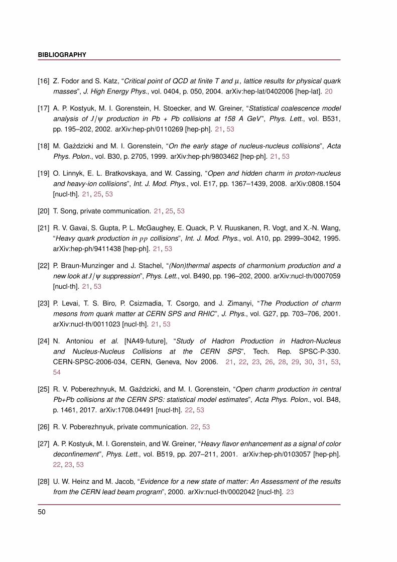
[16] Z. Fodor and S. Katz, “Critical point of QCD at finite T and µ , lattice results for physical quarkmasses”, J. High Energy Phys., vol. 0404, p. 050, 2004. arXiv:hep-lat/0402006 [hep-lat]. 20

[17] A. P. Kostyuk, M. I. Gorenstein, H. Stoecker, and W. Greiner, “Statistical coalescence modelanalysis of J/ψ production in Pb + Pb collisions at 158 A GeV ”, Phys. Lett., vol. B531,pp. 195–202, 2002. arXiv:hep-ph/0110269 [hep-ph]. 21, 53

[18] M. Gazdzicki and M. I. Gorenstein, “On the early stage of nucleus-nucleus collisions”, ActaPhys. Polon., vol. B30, p. 2705, 1999. arXiv:hep-ph/9803462 [hep-ph]. 21, 53

[19] O. Linnyk, E. L. Bratkovskaya, and W. Cassing, “Open and hidden charm in proton-nucleusand heavy-ion collisions”, Int. J. Mod. Phys., vol. E17, pp. 1367–1439, 2008. arXiv:0808.1504[nucl-th]. 21, 25, 53

[20] T. Song, private communication. 21, 25, 53

[21] R. V. Gavai, S. Gupta, P. L. McGaughey, E. Quack, P. V. Ruuskanen, R. Vogt, and X.-N. Wang,“Heavy quark production in pp collisions”, Int. J. Mod. Phys., vol. A10, pp. 2999–3042, 1995.arXiv:hep-ph/9411438 [hep-ph]. 21, 53

[22] P. Braun-Munzinger and J. Stachel, “(Non)thermal aspects of charmonium production and anew look at J/ψ suppression”, Phys. Lett., vol. B490, pp. 196–202, 2000. arXiv:nucl-th/0007059[nucl-th]. 21, 53

[23] P. Levai, T. S. Biro, P. Csizmadia, T. Csorgo, and J. Zimanyi, “The Production of charmmesons from quark matter at CERN SPS and RHIC”, J. Phys., vol. G27, pp. 703–706, 2001.arXiv:nucl-th/0011023 [nucl-th]. 21, 53

[24] N. Antoniou et al. [NA49-future], “Study of Hadron Production in Hadron-Nucleusand Nucleus-Nucleus Collisions at the CERN SPS”, Tech. Rep. SPSC-P-330.CERN-SPSC-2006-034, CERN, Geneva, Nov 2006. 21, 22, 23, 26, 28, 29, 30, 31, 53,54

[25] R. V. Poberezhnyuk, M. Gazdzicki, and M. I. Gorenstein, “Open charm production in centralPb+Pb collisions at the CERN SPS: statistical model estimates”, Acta Phys. Polon., vol. B48,p. 1461, 2017. arXiv:1708.04491 [nucl-th]. 22, 53

[26] R. V. Poberezhnyuk, private communication. 22, 53

[27] A. P. Kostyuk, M. I. Gorenstein, and W. Greiner, “Heavy flavor enhancement as a signal of colordeconfinement”, Phys. Lett., vol. B519, pp. 207–211, 2001. arXiv:hep-ph/0103057 [hep-ph].22, 23, 53

[28] U. W. Heinz and M. Jacob, “Evidence for a new state of matter: An Assessment of the resultsfrom the CERN lead beam program”, 2000. arXiv:nucl-th/0002042 [nucl-th]. 23

50

BIBLIOGRAPHY

[29] H. Satz, “Calibrating the In-Medium Behavior of Quarkonia”, Adv. High Energy Phys., vol. 2013,p. 242918, 2013. 23, 53

[30] M. C. Abreu et al. [NA50, NA38], “Dimuon and charm production in nucleus-nucleus collisionsat the CERN SPS”, Eur. Phys. J., vol. C14, pp. 443–455, 2000. 24

[31] M. C. Abreu et al. [NA50], “Evidence for deconfinement of quarks and gluons from the J/ψsuppression pattern measured in Pb + Pb collisions at the CERN SPS”, Phys. Lett., vol. B477,pp. 28–36, 2000. 24, 53

[32] R. Arnaldi et al. [NA60], “J/ψ production in indium-indium collisions at 158-GeV/nucleon”, Phys.Rev. Lett., vol. 99, p. 132302, 2007. 24

[33] C. Patrignani et al. [Particle Data Group], “The Review of Particle Physics (2017)”. http://pdg.lbl.gov/, Accessed: 18.06.2018. 26, 40, 41, 55

[34] “MIMOSA26 User Manual”. http://www.iphc.cnrs.fr/IMG/pdf/M26_UserManual_light.pdf,Accessed: 17.06.2018. 28

[35] Z.-W. Lin et al., “A Multi-phase transport model for relativistic heavy ion collisions”, Phys. Rev.,vol. C72, p. 064901, 2005. 28

[36] A. Aduszkiewicz et al. [NA61/SHINE], “Beam momentum scan with Pb+Pb collisions”, Tech.Rep. CERN-SPSC-2015-038. SPSC-P-330-ADD-8, CERN, Geneva, Oct 2015. 29, 31, 54

[37] M. Mager [ALICE], “ALPIDE, the Monolithic Active Pixel Sensor for the ALICE ITS upgrade”,Nucl. Instrum. Meth., vol. A824, pp. 434–438, 2016. 30

[38] F. James and M. Winkler, “MINUIT User’s Guide”. http://seal.web.cern.ch/seal/documents/minuit/mnusersguide.pdf, 2004. 33

[39] R. Fruhwirth, “Application of Kalman filtering to track and vertex fitting”, Nucl. Instrum. Meth.,vol. A262, pp. 444–450, 1987. 36

[40] A. Aduszkiewicz et al. [NA61/SHINE], “Report from the NA61/SHINE experiment at the CERNSPS”, Tech. Rep. CERN-SPSC-2017-038. SPSC-SR-221, CERN, Geneva, Oct 2017. 42, 43,45, 55

51

LIST OF FIGURES

List of Figures

1 The table of all elementary particles included in the Standard Model. Figure from Ref.[2]. . . . . . . . . . . . . . . . . . . . . . . . . . . . . . . . . . . . . . . . . . . . . . . . . . 14

2 The summary of fundamental interactions. Figure from Ref. [3]. . . . . . . . . . . . . . 15

3 The schematic picture of confinement effect. Figure from Ref. [4]. . . . . . . . . . . . . 15

4 The space-time evolution of heavy-ion collision. Figure from Ref. [5]. . . . . . . . . . . 16

5 The phase diagram of strongly interacting matter. The gray band corresponds to thefirst order phase transition finished by the critical point. The close points correspond tothe chemical freeze-out and open points to the hypothetical points of the early stageof the collision. Figure from Ref. [11]. . . . . . . . . . . . . . . . . . . . . . . . . . . . . . 18

6 The schematic picture presenting the data collected within system size – beammomentum scan performed by NA61/SHINE. Figure from Ref. [15]. . . . . . . . . . . . 19

7 The coverage of the phase diagram of strongly interacting matter by NA61/SHINEdata. Figure from Ref. [15]. . . . . . . . . . . . . . . . . . . . . . . . . . . . . . . . . . . 20

8 Mean multiplicities of charm quark pairs produced in a full phase-space in centralPb+Pb collisions at 158A GeV/c calculated within statistical models (green bars):the Hadron Resonance Gas model (HRG) [17], the Statistical Quark Coalescencemodel [17] and the Statistical Model of the Early Stage (SMES) [18] as well asdynamical models (blue bars): the Hadron String Dynamics (HSD) model [19, 20],a pQCD-inspired model [21, 22] and the Dynamical Quark Coalescence model [23].Figure from Ref. [24]. . . . . . . . . . . . . . . . . . . . . . . . . . . . . . . . . . . . . . . 21

9 Energy dependence (√

sNN – center of mass energy per nucleon pair) of meanmultiplicity of charm quark pairs according to the Statistical Model of the Early Stage[25, 26]. Dotted line represents scenario without phase transition and solid one withphase transition (the energy of the onset of deconfinement is approximately

√sNN ≈ 7

GeV). Figure from Ref. [24]. . . . . . . . . . . . . . . . . . . . . . . . . . . . . . . . . . . 22

10 Energy dependence of the ratio of mean multiplicity of charm quark pairs indeconfined and confined matter in central Pb+Pb collisions calculated within thepQCD-inspired model [27]. Figure from Ref. [24]. . . . . . . . . . . . . . . . . . . . . . . 23

11 Schematic picture of charm production in p+p collisions (Left) and heavy-ion collisions(Right). Figure from Ref. [29]. . . . . . . . . . . . . . . . . . . . . . . . . . . . . . . . . . 23

12 The branching ratio (B) multiplied σJ/ψ and divided by σDY as a function of transverseenergy (measure of collision centrality) in Pb+Pb collisions at 158A GeV/c measuredby NA50. The curve represents the J/ψ suppression due to ordinary (”cold”) nuclearmatter absorption. Figure from Ref. [31]. . . . . . . . . . . . . . . . . . . . . . . . . . . . 24

13 Total charm distribution over different charm hadrons according to PHSD model [19,20] for Pb+Pb collisions at 158A GeV/c. . . . . . . . . . . . . . . . . . . . . . . . . . . . 25

14 The schematic picture showing the idea behind D0 meson measurement. Figure fromRef. [24]. . . . . . . . . . . . . . . . . . . . . . . . . . . . . . . . . . . . . . . . . . . . . . 26

53

LIST OF FIGURES

15 The schematic picture of the NA61/SHINE detector. Figure from Ref. [15]. . . . . . . . 27

16 The final project (Left) and the photo (Right) of the Small-Acceptance Vertex Detector.Figure from Ref. [24]. . . . . . . . . . . . . . . . . . . . . . . . . . . . . . . . . . . . . . . 28

17 Transverse momentum (momentum in plane perpendicular to beam axis) and rapidity(y = 1

2 ln E+pLE−pL

, where: E – energy, pL = pz – momentum along z axis; yCM – rapidity

calculated in center-of-mass frame) distributions of D0 + D0 mesons produced incentral Pb+Pb collisions at 150A GeV/c simulated within the AMPT model andcorresponding to 3 ⋅106 events. Left : Results for all produced D0 + D0 mesons. Right :results for D0 + D0 mesons fulfilling the following criteria: decay D0

→ π++K− and

D0→ π

−+K+, both decay products registered by the SAVD, passing background

suppression and quality cuts [36]. Figure from Ref. [24]. . . . . . . . . . . . . . . . . . . 29

18 Summary picture of all upgrade plans of the NA61/SHINE detector. Figure from Ref.[24]. . . . . . . . . . . . . . . . . . . . . . . . . . . . . . . . . . . . . . . . . . . . . . . . . 30

19 The picture of the layers of VD based on the ALPIDE sensors. From left to right: thefirst layer with two sensors, the second layer with 8 sensors, the third layer with 12sensors and the fourth layer with 24 sensors. The total active area of the VD sensorsis 190 cm2. Figure from Ref. [24]. . . . . . . . . . . . . . . . . . . . . . . . . . . . . . . . 30

20 The 3D visualization of the VD geometry presented in Fig. 19. Figure from Ref. [24]. . 31

21 Transverse momentum and rapidity distributions of D0 + D0 mesons produced incentral Pb+Pb collisions at 150A GeV/c simulated within the AMPT model andcorresponding to 500 ⋅ 106 events. Left : Results for all produced D0 + D0 mesons.Right : results for D0 + D0 mesons fulfilling the following criteria: decay D0

→ π++K−

and D0→ π

−+K+, both decay products registered by the future NA61/SHINE Vertex

Detector, passing background suppression and quality cuts [36]. Figure from Ref. [24]. 31

22 The definition of the ”dev” variable used for geometry tuning. Vds1, Vds2 and Vds3denote the clusters from first, second and third station of SAVD, respectively. . . . . . 33

23 The naming convention of SAVD sensors. Figure from Ref. [15]. . . . . . . . . . . . . 33

24 Left : The distribution of x residuals between fitted tracks and hits registered by theVds2_0 sensor in the Jura arm. The improvement factor, calculated from Formula (5),is 20%. Right : The distribution of y residuals between fitted tracks and hits registeredby the Vds4_0 sensor in the Saleve arm. The improvement factor, calculated fromFormula (5), is 22%. Distributions before and after final geometry tuning are shownby blue and red histograms, respectively. . . . . . . . . . . . . . . . . . . . . . . . . . . 35

25 The photo of example rotated and shifted sensor. . . . . . . . . . . . . . . . . . . . . . 36

26 Left : Track before refitting to VD primary vertex. The vertexing precision (theuncertainty of reconstructed vertices position) from TPC reconstruction is on the orderof cm. Right : Track after refitting to VD primary vertex. On both plots the coordinatessystem is as introduced in Figure 15. . . . . . . . . . . . . . . . . . . . . . . . . . . . . 37

54

LIST OF FIGURES

27 The distributions of the distances between interpolated tracks and all VD clusters fromfirst station before (Left) and after (Right) refitting to VD primary vertex. It shows thatin order to see the correlation between matching tracks and clusters, the first step ofthe algorithm (see Section 4.2.1) is needed. . . . . . . . . . . . . . . . . . . . . . . . . 38

28 The matched VD clusters to TPC track. . . . . . . . . . . . . . . . . . . . . . . . . . . . 3829 Left : Track before refitting to VD cluster. Right : Track after refitting to VD cluster. . . . 3930 Example of two different secondary tracks matched with VD clusters. . . . . . . . . . 3931 The reconstructed signal of K0

s particle. The black line corresponds to the K0s mass

taken from Ref. [33]. . . . . . . . . . . . . . . . . . . . . . . . . . . . . . . . . . . . . . . 4032 Top Left : K0

s signal obtained from first sample. Top Right : K0s signal obtained from

second sample. Bottom: The comparison of K0s signal obtained from different samples

of data. Data from first sample were scaled by eye. The black line corresponds to theK0

s mass taken from Ref. [33]. . . . . . . . . . . . . . . . . . . . . . . . . . . . . . . . . . 4133 The distribution of the cuts variables from the simulation (AMPT model, Pb+Pb

at 150A GeV/c) for D0+D0 signal (red) and background (blue). The backgrounddistributions were obtained using all the tracks (primary and secondary). Figure fromRef. [40]. . . . . . . . . . . . . . . . . . . . . . . . . . . . . . . . . . . . . . . . . . . . . . 43

34 The distribution of the cuts variables from the reconstructed data. . . . . . . . . . . . 4335 The invariant mass distribution of reconstructed secondary tracks assuming pion and

kaon mass. . . . . . . . . . . . . . . . . . . . . . . . . . . . . . . . . . . . . . . . . . . . 4436 The invariant mass distribution of reconstructed secondary tracks assuming pion

and kaon mass obtained from track matching via extrapolation [40] (Left) and viainterpolation (Right). . . . . . . . . . . . . . . . . . . . . . . . . . . . . . . . . . . . . . . 45

55