Acta Geodyn. Geomater., Vol. 10, No. 4 (172), 443–452, 2013 DOI: 10.13168/AGG.2013.0044

ORIGINAL PAPER

OPTIMAL DATA PROCESSING STRATEGY IN PRECISE GPS LEVELING NETWORKS

Katarzyna STEPNIAK 1)*, Radosław BARYŁA 1), Paweł WIELGOSZ 1) and Grzegorz KURPINSKI 2)

1) University of Warmia and Mazury in Olsztyn, Oczapowskiego 2, Olsztyn, Poland 2) KGHM CUPRUM sp. z o.o. Centrum Badawczo-Rozwojowe, Sikorskiego 2-8, Wrocław, Poland *Corresponding author‘s e-mail: katarzyna.stepniak@uwm.edu.pl (Received February 2013, accepted May 2013) ABSTRACT GPS (Global Positioning System) technique has become a major tool in contemporary surveying and geodesy. This concernsmostly measurements of horizontal point coordinates, where centimeter-level accuracies are usually required and easily achievable. For the height component, however, these requirements are higher and millimeter-level accuracy is necessary. On the other hand, the intrinsic precision of GPS-derived heights is clearly lower comparing to the horizontal components. This isdue to unfavorable satellite geometry, adverse effects of the troposphere or GPS antenna phase center offset and variations. Inorder to overcome these effects one has to carefully model all the error sources and rigorously process the GPS data. This paper presents studies on the optimal GPS data processing strategy suitable for precise leveling. This was done throughthe extensive testing and selection of the most appropriate observational session duration, ambiguity resolution strategy, network geometry, troposphere and ionospheric delay reduction methods, signal linear combination, elevation angle cut-off, etc. The analyzed processing strategies were evaluated through the processing of a test network. The test network consisted of 19 monitored points and 5 control points, and covered the area of 20 km x 60 km. The obtained results show that the precise GPS leveling with the selected optimal processing strategy allows for about 3 mm repeatability of height measurements when processing 4-hour long sessions. In our opinion GPS leveling may serve as fast and cost-effective replacement of classic geometric leveling, especially in applications where the heights in orthometric or normal height systems are not necessary. This is the case in, e.g., ground deformation studies. KEYWORDS: GPS, precise GPS leveling, post-processing

models for reduction of the ionospheric and tropospheric refraction have to be applied (Grejner-Brzezinska et al., 2007; Bosy et al., 2011). Hardware biases, including satellite and receiver antenna phase center variations as well as errors related to thecorrect antenna centering over a surveyed point, need to be eliminated (Görres et al., 2006).

In this paper, studies on the optimal processing strategy of GPS data in precise satellite leveling are presented. Bernese GPS processing software ver. 5.0 was applied in all the numerical tests (Dach et al.,2007). The main focus was set on optimal processing parameter selection, including session duration, sampling interval, elevation mask, elimination of the tropospheric and ionospheric delays, network geometry, etc. When selecting the test leveling network, the assumption was that the distances between the network nodes were in the range of 5-10 km. These distances are standard in the leveling networks established for monitoring ground deformations in the mining activity areas. 2. TEST DATA

For the analysis a test area of 20x60 km was selected (Fig. 1). The test area covers a part of the leveling network established for ground deformation monitoring in one of the largest copper mining region in Europe – LGOM (Legnica-Głogów Copper Belt), which is located in Poland. In this region the mining

1. INTRODUCTION

In the last decade of the XX century, a new era in geodetic surveys began through the dissemination of precise satellite measurements. The steady improvement of the satellite measurement techniques has motivated increase of the accuracy of the resulting coordinates to millimeter and submillimeter level (Leick, 2004; Cellmer et al., 2010; Wielgosz, 2011; Bakula, 2012). Nowadays, satellite measurements are of great importance in monitoring the deformations of the Earth's crust, which have resulted from the impact of natural forces and human activities. The example of human activities that cause surface deformations is mining activity. Several research groups have conducted the studies of using satellite measurements to determine the deformation parameters on the area of Central Europe (e.g. Pospíšil et al., 2010, Blachowski et al., 2010; Bogusz et al., 2013). Some of these studies have also been made by University of Warmia and Mazury in Olsztyn (Wielgosz et al.,2011; Kamiński and Nowel, 2013). The achieved results show the possibility of replacing the classic leveling measurements with precise GPS (Global Positioning System) / GNSS (Global Navigation Satellite System) measurements. This, however, requires the state of the art equipment and data processing software and algorithms. Also, systematic errors need to be eliminated or at least greatlyreduced. Therefore, advanced signal propagation

K. Stępniak et al.

444

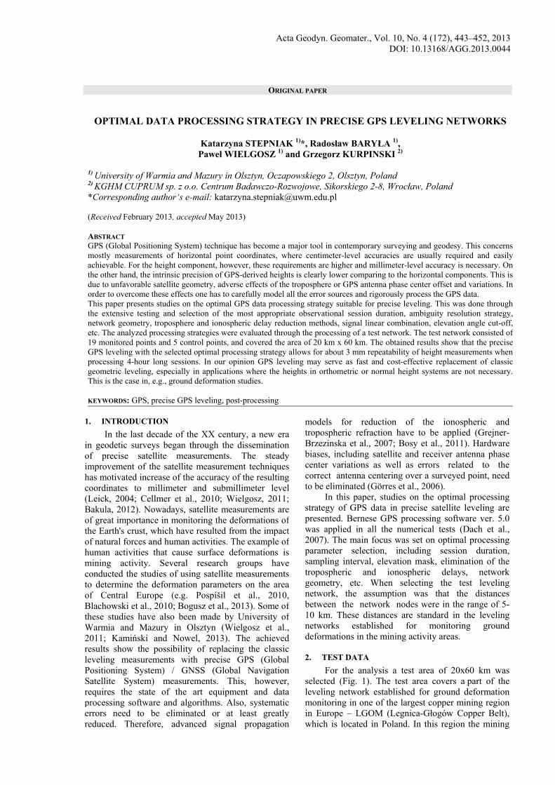
Fig. 1 Location of the test area in Poland and locations of the reference and control points.

sessions – eight hours each. The satellite measurements were performed with the following assumptions:

GNSS receivers: 16 sets,

length of the observing sessions at the reference points: 8 hours,

length of the observing sessions at the monitoredpoints: 8 hours,

number of the observing session at the reference points: 5,

number of the observing session at the monitoredpoints: 1 or 2,

GPS frequency: L1 & L2,

GPS measurements: pseudorange and carrier-phases,

interval: 5 s,

elevation mask: 0˚,

maximum value of PDOP: 6,

forced centering of the satellite antenna on leveling benchmarks with a special device.

3. NUMERICAL TESTS AND PROCESSING

STRATEGIES

The use of commercial software, which is provided by the equipment manufacturer for processing satellite observations, limits the ability to modify the processing parameters. This, in turn, limits the possibilities of using advanced error models and, therefore, limits the ability to improve the accuracy ofthe derived position. For advanced and precise data processing it is recommended to use software which enables almost limitless selection of the processing parameters and error models. Therefore, as it has

subsidence rate amounts to 30-40 cm per year. Simultaneous classic geometric and satellite leveling measurements were carried out at two classic leveling lines including 19 nodal (monitored) points (denoted as PP and LL) and 5 control points (first class benchmarks, denoted RR). Two of the monitored points – LL01 and LL02 – were used to connect both leveling lines, hence, these two points were surveyed in all sessions during the test campaign. Additionally,GPS data from several reference stations of the Polish national Ground Based Augmentation System(GBAS) network – ASG-EUPOS – were used. The selected test area is rather flat with normal heights of the control points varied from 88.596 m to 178.560 m. The normal heights of the monitored points varied from 90.725 m to 175.918 m.

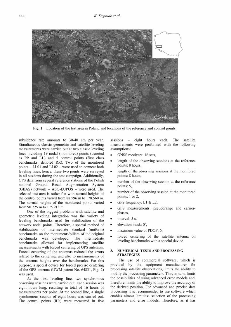
One of the biggest problems with satellite and geometric leveling integration was the variety of leveling benchmarks used for stabilization of the network nodal points. Therefore, a special method of stabilization of intermediate standard (uniform) benchmarks on the monuments/pillars of the original benchmarks was developed. The intermediate benchmarks allowed for implementing satellite measurements with forced centering of GPS antennas. Forced centering of the antennas reduced the errors related to the centering, and also to measurements ofthe antenna heights over the benchmarks. For this purpose, a special device for forced precise centering of the GPS antenna (UWM patent No. 64831, Fig. 2)was used.

At the first leveling line, two synchronous observing sessions were carried out. Each session was eight hours long, resulting in total of 16 hours of measurements per point. At the second line, a singlesynchronous session of eight hours was carried out. The control points (RR) were measured in five

OPTIMAL DATA PROCESSING STRATEGY IN PRECISE GPS LEVELING NETWORKS

.

445

Fig. 2 Special device for forced precise centering of the GPS antenna.

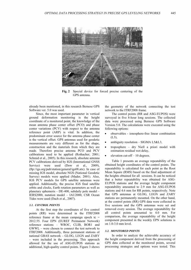
the geometry of the network connecting the test network to the ITRF2008 frame.

The control points (RR and ASG-EUPOS) were surveyed in five 8-hour long sessions. The collected data were processed using Bernese GPS Software Version 5.0. The calculations were executed using the following options:

observables - ionosphere-free linear combination (L3),

ambiguity resolution – SIGMA L5&L3,

troposphere – dry Niell a priori model with estimation residual wet delay,

elevation cut-off – 10 degrees.

Table 1 presents an average repeatability of the obtained height coordinates of the control points. The repeatability is calculated for each point as the Root Mean Square (RMS) based on the final adjustment of the heights obtained for all sessions. It can be noticed that a better repeatability was obtained for ASG-EUPOS stations and the average height component repeatability amounted to 2.9 mm for ASG-EUPOS stations and 4.6 mm for RR points, respectively. Note that GPS antennas at GLOG, LEGN and ZARY stations are permanently mounted. On the other hand, at the control points (RR) GPS data were collected in five sessions and the GPS antennas were set and removed every session. The average repeatability for all control points amounted to 4.0 mm. For comparison, the average repeatability of the height component presented in the weekly EPN solutions is on 1.0-3.0 mm level.

3.2. MONITORED POINTS

In order to analyze the achievable accuracy of the height component derived from the processing ofGPS data collected at the monitored points, several processing strategies and options were tested. This

already been mentioned, in this research Bernese GPS Software ver. 5.0 was used.

Since, the most important parameter in vertical ground deformation monitoring is the height coordinate of a monitored point, the knowledge of the mean antenna phase center offset (PCO) and phase center variations (PCV) with respect to the antenna reference point (ARP) is vital. In addition, the predominant error source for the antenna phase center is the vertical offset. GPS antennas used for geodetic measurements are very different as for the shape, construction and the materials from which they are made. Therefore precise antenna PCO and PCV calibrations need to be applied (Rothacher, 2001; Schmid et al., 2005). In this research, absolute antenna PCV calibrations derived by IGS (International GNSS Service) were used (Dow et al., 2009), (ftp://igs.org/pub/station/general/igs08.atx). In case of missing IGS model, absolute NGS (National Geodetic Survey) models were applied (Mader, 2001). Also, IGS PCV models for GPS satellite antennas were applied. Additionally, the precise IGS final satellite orbits and clocks, Earth rotation parameters as well as planetary ephemeris – DE-400, subdaily pole model –IERS2000, nutation model – IAU2000, CSR Ocean Tides were used (Dach et al., 2007). 3.1. CONTROL POINTS

At the first step the coordinates of five control points (RR) were determined in the ITRF2008 reference frame at the mean campaign epoch tc = 2012.55. Four EPN (EUREF Permanent Network) reference stations – WROC, CLIB, BOR1 and GWWL – were chosen to connect the test network to ITRF2008. Additionally, three permanent stations of national GBAS network – GLOG, LEGN and ZARY – were included in the processing. This approach allowed for the use of ASG-EUPOS stations as additional, high-quality control points. Figure 3 shows

K. Stępniak et al.

446

EPN-ASG-RR [mm] RR01 4.9 RR02 4.9 RR03 6.3 RR04 3.0 RR05 4.4 average (RR) 4.6 GLOG 3.8 LEGN 2.3 ZARY 2.7 average (ASG) 2.9 average (all) 4.0

Table 1 Average height repeatability at reference points (based on processing five 8-hour sessions).

Fig. 3 The geometry of the network connecting the test network to the ITRF2008 frame.

includes testing the influence of the following parameters:

geometry – “star”-shaped network or polygon;

observing session length – 8 hours, 4 hours,2 hours;

ionosphere model – CODE global model or without ionosphere information;

frequency – L1 (with ionosphere model) or iono-free linear combination (L3);

troposphere modeling - a priori Niell with estimation of the residual wet delays with wet Niell mapping function, different constraints (sigma a priori) tested;

satellite elevation cut-off: 5˚, 10˚; 15 ˚; ambiguity resolution – SIGMA L1 or SIGMA

L5&L3.

In addition, as it has already been mentionedabove, the IGS precise products were applied. Overall, more than 80 processing strategies were tested and verified. In this paper, however, the results of only 18selected tests are presented.

All the studies presented below were referred to the “reference” strategy that used the following “reference” options:

observing session length – 4 hours,

frequency – L1 with CODE global ionosphere model,

troposphere modeling - a priori Niell model with tightly constrained residual wet delays (sigma a priori = 0.0001 m),

satellite elevation cut-off: 5˚. 3.2.1. NETWORK GEOMETRY

Due to a large span of the test network and the fact that it serves for two purposes: (1) measurementsof a few selected monitored points in the area of sudden geotectonic event, and (2) periodic monitoring of the whole network for the deformation analysis, we propose two variants of the control network geometry:

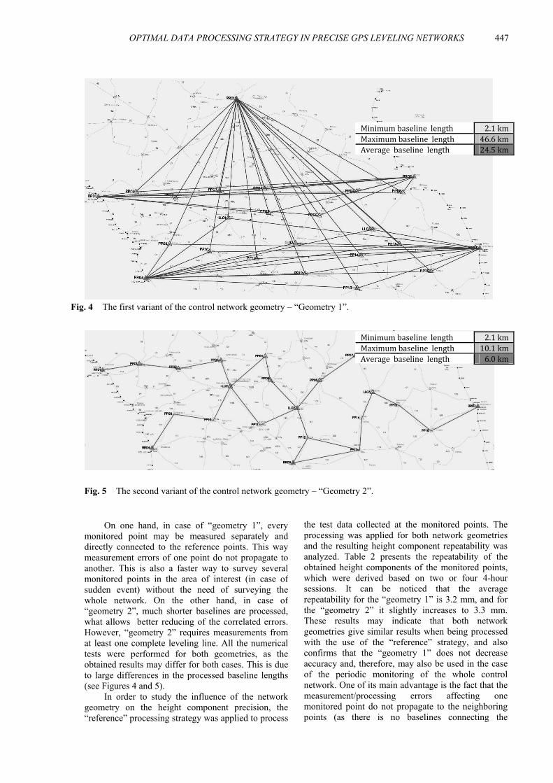
1. „geometry 1” - network connecting each monitored point separately to 3 control points, without any baselines between the monitored points, all the baselines are processed in a common data adjustment (Fig. 4) – this is a case of surveying the sudden incidents effects,

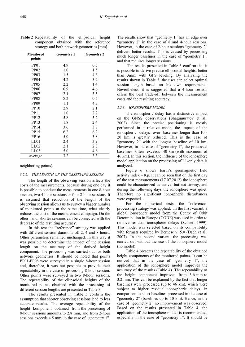
2. „geometry 2” - reflecting regular leveling lines with baselines connecting neighboring monitored points (Fig. 5) – this is a case of periodic monitoring of the whole network.

OPTIMAL DATA PROCESSING STRATEGY IN PRECISE GPS LEVELING NETWORKS

.

447

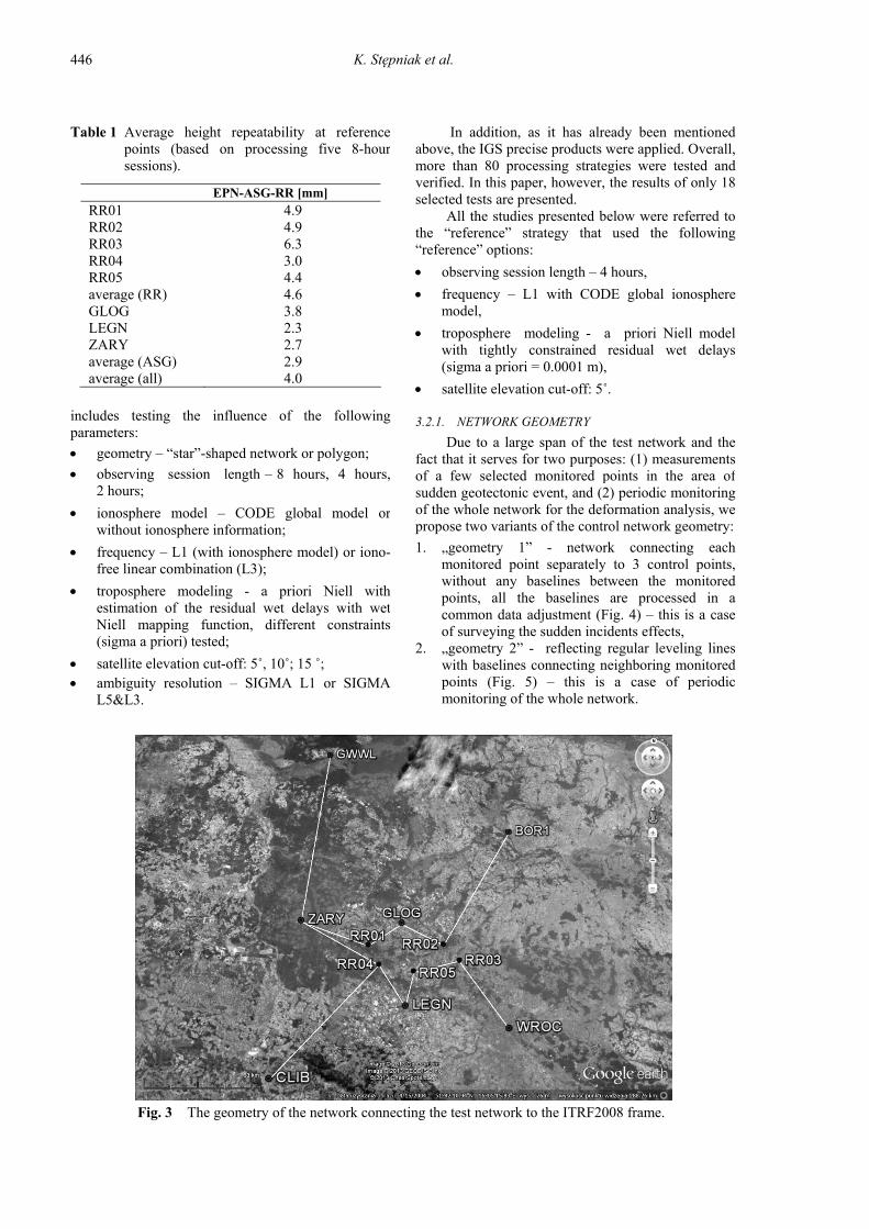
Minimumbaselinelength 2.1kmMaximumbaselinelength 46.6kmAveragebaselinelength 24.5km

Minimumbaselinelength 2.1kmMaximumbaselinelength 10.1kmAveragebaselinelength 6.0km

Fig. 4 The first variant of the control network geometry – “Geometry 1”.

Fig. 5 The second variant of the control network geometry – “Geometry 2”.

the test data collected at the monitored points. The processing was applied for both network geometries and the resulting height component repeatability was analyzed. Table 2 presents the repeatability of the obtained height components of the monitored points, which were derived based on two or four 4-hour sessions. It can be noticed that the average repeatability for the “geometry 1” is 3.2 mm, and for the “geometry 2” it slightly increases to 3.3 mm. These results may indicate that both network geometries give similar results when being processed with the use of the “reference” strategy, and also confirms that the “geometry 1” does not decrease accuracy and, therefore, may also be used in the case of the periodic monitoring of the whole control network. One of its main advantage is the fact that the measurement/processing errors affecting one monitored point do not propagate to the neighboring points (as there is no baselines connecting the

On one hand, in case of “geometry 1”, every monitored point may be measured separately and directly connected to the reference points. This way measurement errors of one point do not propagate to another. This is also a faster way to survey several monitored points in the area of interest (in case of sudden event) without the need of surveying the whole network. On the other hand, in case of “geometry 2”, much shorter baselines are processed, what allows better reducing of the correlated errors. However, “geometry 2” requires measurements from at least one complete leveling line. All the numerical tests were performed for both geometries, as the obtained results may differ for both cases. This is due to large differences in the processed baseline lengths(see Figures 4 and 5).

In order to study the influence of the network geometry on the height component precision, the “reference” processing strategy was applied to process

K. Stępniak et al.

448

Table 2 Repeatability of the ellipsoidal heightcomponent obtained with the reference strategy and both network geometries [mm].

Monitored points

Geometry 1 Geometry 2

PP01 4.9 0.5 PP02 1.0 1.5 PP03 1.5 4.6 PP04 4.2 3.2 PP05 2.2 1.4 PP06 0.9 4.6 PP07 2.1 3.5 PP08 8.2 0.5 PP09 1.1 4.2 PP10 2.9 2.1 PP11 1.0 2.2 PP12 5.8 5.2 PP13 1.8 2.4 PP14 3.6 3.8 PP15 6.2 6.2 PP16 5.0 3.8 LL01 2.4 3.9 LL02 2.1 2.8 LL03 5.0 4.6

average 3.2 3.3 neighboring points).

3.2.2. THE LENGTH OF THE OBSERVING SESSION

The length of the observing session affects the costs of the measurements, because during one day it is possible to conduct the measurements in one 8-hour session, two 4-hour sessions or four 2-hour sessions. It is assumed that reduction of the length of the observing session allows us to survey a bigger number of monitored points at the same time, what clearly reduces the cost of the measurement campaign. On the other hand, shorter sessions can be connected with the decrease of the resulting accuracy.

In this test the “reference” strategy was applied with different session durations of: 2, 4 and 8 hours. Other parameters remained unchanged. In this way it was possible to determine the impact of the session length on the accuracy of the derived height component. The processing was carried out for both network geometries. It should be noted that points PP01-PP08 were surveyed in a single 8-hour session and, therefore, it was not possible to provide their repeatability in the case of processing 8-hour session. Other points were surveyed in two 8-hour sessions. The repeatability of the ellipsoidal heights of the monitored points obtained with the processing of different session lengths are presented in Table 3.

The results presented in Table 3 confirm the assumption that shorter observing sessions lead to less accurate results. The average repeatability of the height komponent obtained from the processing of 8-hour sessions amounts to 2.8 mm, and from 2-hour sessions exceeds 4.5 mm, in the case of “geometry 1”.

The results show that “geometry 1” has an edge over “geometry 2” in the case of 8 and 4-hour sessions. However, in the case of 2-hour sessions “geometry 2” delivers better results. This is caused by processing much longer baselines in the case of “geometry 1”, and that requires longer sessions.

The results presented in Table 3 confirm that it is possible to derive precise ellipsoidal heights, better than 3mm, with GPS leveling. By analyzing the results shown in Table 3, the user can select optimal session length based on his own requirements. Nevertheless, it is suggested that a 4-hour session offers the best trade-off between the measurement costs and the resulting accuracy.

3.2.3. IONOSPHERE MODEL

The ionospheric delay has a distinctive impact on the GNSS observations (Shagimuratov et al., 2002). Since the precise positioning is mostlyperformed in a relative mode, the impact of the ionospheric delays over baselines longer than 10 -20 km is greatly reduced. This is the case of “geometry 2” with the longest baseline of 10 km. However, in the case of “geometry 1”, the processed baselines often exceeds 40 km (with maximum of 46 km). In this section, the influence of the ionosphere model application on the processing of L1-only data is analyzed.

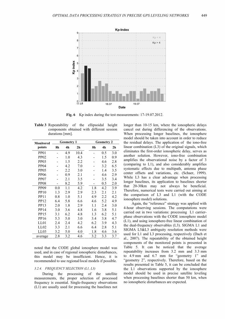
Figure 6 shows Earth’s geomagnetic field activity index – Kp. It can be seen that on the first day of the test measurements (17.07.2012) the ionosphere could be characterized as active, but not stormy, and during the following days the ionosphere was quiet.Therefore no significant ionospheric disturbances were expected.

For the numerical tests, the “reference” processing strategy was applied. In the first variant, a global ionosphere model from the Centre of Orbit Determination in Europe (CODE) was used in order to remove residual ionospheric delays (Schaer, 1999).This model was selected based on its compatibility with formats required by Bernese v. 5.0 (Dach et al., 2007). In the second variant, the processing was carried out without the use of the ionosphere model (no model).

Table 4 presents the repeatability of the obtained height components of the monitored points. It can be noticed that in the case of „geometry 1”, the application of the ionosphere model improves the accuracy of the results (Table 4). The repeatability of the height component improved from 3.6 mm to 3.2 mm. This can be explained by the fact that longer baselines were processed (up to 46 km), which were subject to higher residual ionospheric delays, in comparison to short baselines processed in the case of “geometry 2” (baselines up to 10 km). Hence, in the case of “geometry 2” no improvement was observed. Based on the results presented in Table 4, the application of the ionosphere model is recommended, especially in the case of “geometry 1”. It should be

OPTIMAL DATA PROCESSING STRATEGY IN PRECISE GPS LEVELING NETWORKS

.

449

10

1

2

3

4

5

6

7

8

9Kp-Index

Date

Kp

ind

ex

18.07 19.0717.07

Kp > 4

Kp < 4

Fig. 6 Kp index during the test measurements: 17-19.07.2012.

Table 3 Repeatability of the ellipsoidal heightcomponents obtained with different session durations [mm].

Geometry 1 Geometry 2 Monitored points 8h 4h 2h 8h 4h 2h

PP01 - 4.9 10.4 - 0.5 3.0 PP02 - 1.0 4.3 - 1.5 0.9 PP03 - 1.5 2.2 - 4.6 2.8 PP04 - 4.2 7.0 - 3.2 6.5 PP05 - 2.2 3.0 - 1.4 3.5 PP06 - 0.9 2.1 - 4.6 2.9 PP07 - 2.1 3.5 - 3.5 3.4 PP08 - 8.2 5.9 - 0.5 2.0 PP09 0.0 1.1 4.2 1.8 4.2 3.9 PP10 1.3 2.9 2.9 2.3 2.1 2.1 PP11 0.8 1.0 5.1 4.9 2.2 4.2 PP12 6.4 5.8 6.6 4.6 5.2 4.9 PP13 2.0 1.8 2.9 1.1 2.4 3.0 PP14 3.0 3.6 4.8 1.6 3.8 5.1 PP15 3.1 6.2 4.8 1.3 6.2 5.1 PP16 5.3 5.0 3.0 3.4 3.8 4.7 LL01 2.4 2.4 4.2 6.2 3.9 4.3 LL02 3.3 2.1 6.6 6.4 2.8 5.1 LL03 3.2 5.0 4.0 1.8 4.6 3.6

average 2.8 3.2 4.6

3.2 3.3 3.7

noted that the CODE global ionosphere model was used, and in case of regional ionospheric disturbances, this model may be insufficient. Hence, it is recommended to use regional/local models if possible.

3.2.4. FREQUENCY SELECTION (L1, L3)

During the processing of the satellite measurements, the proper selection of processed frequency is essential. Single-frequency observations(L1) are usually used for processing the baselines not

longer than 10-15 km, where the ionospheric delays cancel out during differencing of the observations.When processing longer baselines, the ionosphere model should be taken into account in order to reduce the residual delays. The application of the iono-free linear combination (L3) of the original signals, which eliminates the first-order ionospheric delay, serves as another solution. However, iono-free combination amplifies the observational noise by a factor of 3 (comparing to L1), and also considerably amplifies systematic effects due to multipath, antenna phase center offsets and variations, etc. (Schaer, 1999). While L3 has a clear advantage when processing longer baselines, its application to baselines shorter that 20-30km may not always be beneficial. Therefore, numerical tests were carried out aiming at the comparison of L3 and L1 (with the CODE ionosphere model) solutions.

Again, the “reference” strategy was applied with 4-hour observing sessions. The computations were carried out in two variations: processing L1 carrier-phase observations with the CODE ionosphere model (L1), and using ionosphere-free linear combination of the dual-frequency observables (L3). SIGMA L1 and SIGMA L5&L3 ambiguity resolution methods were used for L1 and L3 processing, respectively (Dach et al., 2007). The repeatability of the obtained height components of the monitored points is presented in Table 5. It can be noticed that the average repeatability increases from 3.2 mm and 3.3 mm to 4.9 mm and 6.7 mm for “geometry 1” and “geometry 2”, respectively. Therefore, based on the results presented in Table 5, it can be concluded that the L1 observations supported by the ionosphere model should be used in precise satellite levelingwhen processing baselines shorter than 50 km, when no ionospheric disturbances are expected.

K. Stępniak et al.

450

Table 4 Repeatability of the ellipsoidal heightcomponents obtained with or without the ionosphere model [mm].

Geometry 1 Geometry 2 Monitored points CODE no model CODE no model

PP01 4.9 5.0 0.5 1.9 PP02 1.0 0.9 1.5 0.4 PP03 1.5 1.0 4.6 1.2 PP04 4.2 4.8 3.2 4.7 PP05 2.2 3.5 1.4 3.9 PP06 0.9 0.5 4.6 2.2 PP07 2.1 2.7 3.5 4.9 PP08 8.2 7.5 0.5 3.2 PP09 1.1 0.7 4.2 3.5 PP10 2.9 2.2 2.1 2.2 PP11 1.0 1.4 2.2 3.3 PP12 5.8 6.6 5.2 4.9 PP13 1.8 2.6 2.4 1.8 PP14 3.6 4.1 3.8 2.8 PP15 6.2 6.5 6.2 5.6 PP16 5.0 5.7 3.8 4.1 LL01 2.4 3.2 3.9 4.1 LL02 2.1 2.1 2.8 4.4 LL03 5.0 5.2 4.6 3.7

average 3.2 3.6

3.3 3.3

Table 5 Repeatability of the ellipsoidal height components obtained with the processing of L1 and L3 signals [mm].

Geometry 1 Geometry 2 Monitored points L1 L3 L1 L3

PP01 4.9 2.5 0.5 5.9 PP02 1.0 4.6 1.5 4.1 PP03 1.5 0.8 4.6 9.2 PP04 4.2 8.6 3.2 5.3 PP05 2.2 3.7 1.4 11.2 PP06 0.9 0.6 4.6 4.2 PP07 2.1 3.8 3.5 7.7 PP08 8.2 6.9 0.5 0.9 PP09 1.1 4.0 4.2 5.5 PP10 2.9 4.9 2.1 9.0 PP11 1.0 5.3 2.2 8.9 PP12 5.8 10.4 5.2 9.3 PP13 1.8 7.2 2.4 2.8 PP14 3.6 4.6 3.8 2.2 PP15 6.2 9.7 6.2 8.1 PP16 5.0 7.9 3.8 6.8 LL01 2.4 5.1 3.9 7.3 LL02 2.1 4.4 2.8 11.6 LL03 5.0 8.8 4.6 7.0

average 3.2 4.9

3.3 6.7

the rest of control points and the monitored points it was set to 0.0010 m,

Strategy 2b – “geometry 2” – a priori sigma for the first point of a baseline point was set to 0.0001 m, and for the second point it was set to 0.0010 m,

Strategy 3a – “geometry 1” – a priori sigma at a single control point was set to 0.0001 m, and for the rest of control points and the monitored points it was set to 0.0100 m,

Strategy 3b – “geometry 2” – a priori sigma for the first point of a baseline point was set to 0.0001 m, and for the second point it was set to 0.0100 m.

Strategy 1 presents the tightly constrained solution, whereas Strategy 3 presents the most loosely constrained solution among the tested strategies.

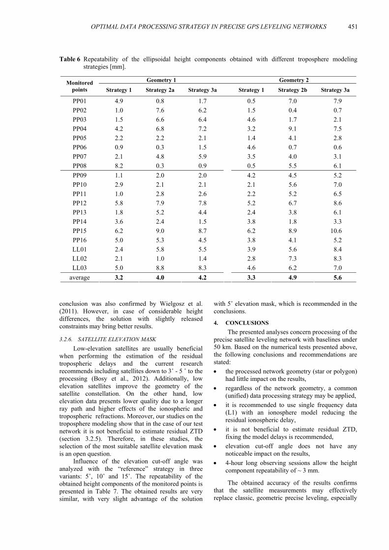
Table 6 includes repeatability of the ellipsoidal height components of the monitored points obtained using the tested strategies. The best results were obtained for the tightly constrained solution, effectively fixing the a priori (model) ZTD. Releasing the constraints imposed on the a priori ZTD results in worsening of the results. This means that in case of flat areas (normal heights of the network points ranged from 88.596 m to 178.560 m) and baselines under 50 km, the estimation of the residual ZTD is not efficient. Therefore, it is concluded that the strategy 1 for the troposphere modeling is optimal and should be applied in the precise satellite leveling. This

3.2.5. TROPOSPHERE MODELING

The study on the troposphere modeling aimed at selection of the optimal strategy for the reduction of the tropospheric delay. The tropospheric refraction is one of the main sources of errors reducing the accuracy of the GNSS-derived height component. This is due to the high correlation between the zenith tropospheric delay (ZTD) and the height coordinate, amounting to over 90 %. Therefore, it is difficult toseparate the tropospheric delays from the height of themeasured point. It is recommended to model the hydrostatic (dry) component of the tropospheric path delay using the Dry Niell model, and then to estimate the non-hydrostatic (wet) delay component using Wet Niell mapping function (Niell, 1996; Bosy et al., 2010). This, however, requires processing of long baselines. Since in the test network the baselines do not exceed 50 km, we focused on testing relative troposphere estimation with ZTD at a single station constrained tightly every time (Dach et al., 2007; Wielgosz et al., 2011). Several processing strategies for the troposphere modeling available in the Bernese software were applied and tested:

Strategy 1 – common for “geometry 1” and “geometry 2” – a priori sigma for ZTD was set to 0.0001m at all the processed points (control and monitored) – resulting in tightly constrained (fixed) ZTD solution,

Strategy 2a – “geometry 1” – a priori sigma at a single control point was set to 0.0001 m, and for

OPTIMAL DATA PROCESSING STRATEGY IN PRECISE GPS LEVELING NETWORKS

.

451

with 5˚ elevation mask, which is recommended in the conclusions.

4. CONCLUSIONS

The presented analyses concern processing of the precise satellite leveling network with baselines under 50 km. Based on the numerical tests presented above, the following conclusions and recommendations are stated:

the processed network geometry (star or polygon) had little impact on the results,

regardless of the network geometry, a common (unified) data processing strategy may be applied,

it is recommended to use single frequency data (L1) with an ionosphere model reducing the residual ionospheric delay,

it is not beneficial to estimate residual ZTD, fixing the model delays is recommended,

elevation cut-off angle does not have any noticeable impact on the results,

4-hour long observing sessions allow the height component repeatability of ~ 3 mm.

The obtained accuracy of the results confirms that the satellite measurements may effectively replace classic, geometric precise leveling, especially

conclusion was also confirmed by Wielgosz et al.(2011). However, in case of considerable height differences, the solution with slightly released constraints may bring better results.

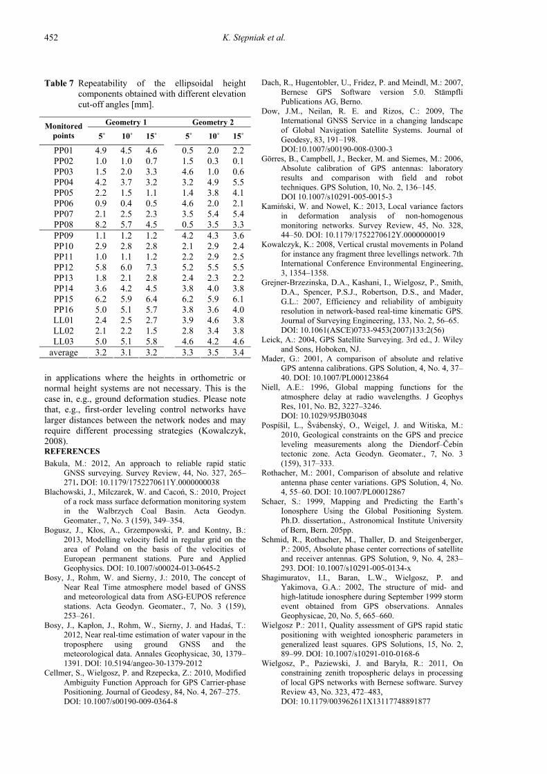
3.2.6. SATELLITE ELEVATION MASK

Low-elevation satellites are usually beneficial when performing the estimation of the residual tropospheric delays and the current research recommends including satellites down to 3˚ - 5 ˚ to the processing (Bosy et al., 2012). Additionally, low elevation satellites improve the geometry of the satellite constellation. On the other hand, low elevation data presents lower quality due to a longer ray path and higher effects of the ionospheric and tropospheric refractions. Moreover, our studies on the troposphere modeling show that in the case of our test network it is not beneficial to estimate residual ZTD (section 3.2.5). Therefore, in these studies, the selection of the most suitable satellite elevation mask is an open question.

Influence of the elevation cut-off angle was analyzed with the “reference” strategy in threevariants: 5˚, 10˚ and 15˚. The repeatability of the obtained height components of the monitored points is presented in Table 7. The obtained results are very similar, with very slight advantage of the solution

Table 6 Repeatability of the ellipsoidal height components obtained with different troposphere modelingstrategies [mm].

Geometry 1 Geometry 2 Monitored points Strategy 1 Strategy 2a Strategy 3a Strategy 1 Strategy 2b Strategy 3a

PP01 4.9 0.8 1.7 0.5 7.0 7.9

PP02 1.0 7.6 6.2 1.5 0.4 0.7

PP03 1.5 6.6 6.4 4.6 1.7 2.1

PP04 4.2 6.8 7.2 3.2 9.1 7.5

PP05 2.2 2.2 2.1 1.4 4.1 2.8

PP06 0.9 0.3 1.5 4.6 0.7 0.6

PP07 2.1 4.8 5.9 3.5 4.0 3.1

PP08 8.2 0.3 0.9 0.5 5.5 6.1

PP09 1.1 2.0 2.0 4.2 4.5 5.2

PP10 2.9 2.1 2.1 2.1 5.6 7.0

PP11 1.0 2.8 2.6 2.2 5.2 6.5

PP12 5.8 7.9 7.8 5.2 6.7 8.6

PP13 1.8 5.2 4.4 2.4 3.8 6.1

PP14 3.6 2.4 1.5 3.8 1.8 3.3

PP15 6.2 9.0 8.7 6.2 8.9 10.6

PP16 5.0 5.3 4.5 3.8 4.1 5.2

LL01 2.4 5.8 5.5 3.9 5.6 8.4

LL02 2.1 1.0 1.4 2.8 7.3 8.3

LL03 5.0 8.8 8.3 4.6 6.2 7.0

average 3.2 4.0 4.2

3.3 4.9 5.6

K. Stępniak et al.

452

1.

Table 7 Repeatability of the ellipsoidal height components obtained with different elevation cut-off angles [mm].

Geometry 1 Geometry 2 Monitored points 5˚ 10˚ 15˚ 5˚ 10˚ 15˚

PP01 4.9 4.5 4.6 0.5 2.0 2.2 PP02 1.0 1.0 0.7 1.5 0.3 0.1 PP03 1.5 2.0 3.3 4.6 1.0 0.6 PP04 4.2 3.7 3.2 3.2 4.9 5.5 PP05 2.2 1.5 1.1 1.4 3.8 4.1 PP06 0.9 0.4 0.5 4.6 2.0 2.1 PP07 2.1 2.5 2.3 3.5 5.4 5.4 PP08 8.2 5.7 4.5 0.5 3.5 3.3 PP09 1.1 1.2 1.2 4.2 4.3 3.6 PP10 2.9 2.8 2.8 2.1 2.9 2.4 PP11 1.0 1.1 1.2 2.2 2.9 2.5 PP12 5.8 6.0 7.3 5.2 5.5 5.5 PP13 1.8 2.1 2.8 2.4 2.3 2.2 PP14 3.6 4.2 4.5 3.8 4.0 3.8 PP15 6.2 5.9 6.4 6.2 5.9 6.1 PP16 5.0 5.1 5.7 3.8 3.6 4.0 LL01 2.4 2.5 2.7 3.9 4.6 3.8 LL02 2.1 2.2 1.5 2.8 3.4 3.8 LL03 5.0 5.1 5.8 4.6 4.2 4.6

average 3.2 3.1 3.2

3.3 3.5 3.4

in applications where the heights in orthometric or normal height systems are not necessary. This is the case in, e.g., ground deformation studies. Please note that, e.g., first-order leveling control networks have larger distances between the network nodes and may require different processing strategies (Kowalczyk, 2008). REFERENCES

Bakula, M.: 2012, An approach to reliable rapid static GNSS surveying. Survey Review, 44, No. 327, 265–271. DOI: 10.1179/1752270611Y.0000000038

Blachowski, J., Milczarek, W. and Cacoń, S.: 2010, Project of a rock mass surface deformation monitoring system in the Walbrzych Coal Basin. Acta Geodyn. Geomater., 7, No. 3 (159), 349–354.

Bogusz, J., Kłos, A., Grzempowski, P. and Kontny, B.: 2013, Modelling velocity field in regular grid on the area of Poland on the basis of the velocities of European permanent stations. Pure and Applied Geophysics. DOI: 10.1007/s00024-013-0645-2

Bosy, J., Rohm, W. and Sierny, J.: 2010, The concept of Near Real Time atmosphere model based of GNSS and meteorological data from ASG-EUPOS reference stations. Acta Geodyn. Geomater., 7, No. 3 (159), 253–261.

Bosy, J., Kapłon, J., Rohm, W., Sierny, J. and Hadaś, T.: 2012, Near real-time estimation of water vapour in the troposphere using ground GNSS and the meteorological data. Annales Geophysicae, 30, 1379–1391. DOI: 10.5194/angeo-30-1379-2012

Cellmer, S., Wielgosz, P. and Rzepecka, Z.: 2010, Modified Ambiguity Function Approach for GPS Carrier-phase Positioning. Journal of Geodesy, 84, No. 4, 267–275. DOI: 10.1007/s00190-009-0364-8

Dach, R., Hugentobler, U., Fridez, P. and Meindl, M.: 2007, Bernese GPS Software version 5.0. Stämpfli Publications AG, Berno.

Dow, J.M., Neilan, R. E. and Rizos, C.: 2009, The International GNSS Service in a changing landscape of Global Navigation Satellite Systems. Journal of Geodesy, 83, 191–198. DOI:10.1007/s00190-008-0300-3

Görres, B., Campbell, J., Becker, M. and Siemes, M.: 2006, Absolute calibration of GPS antennas: laboratory results and comparison with field and robot techniques. GPS Solution, 10, No. 2, 136–145. DOI 10.1007/s10291-005-0015-3

Kamiński, W. and Nowel, K.: 2013, Local variance factors in deformation analysis of non-homogenous monitoring networks. Survey Review, 45, No. 328, 44–50. DOI: 10.1179/1752270612Y.0000000019

Kowalczyk, K.: 2008, Vertical crustal movements in Poland for instance any fragment three levellings network. 7th International Conference Environmental Engineering, 3, 1354–1358.

Grejner-Brzezinska, D.A., Kashani, I., Wielgosz, P., Smith, D.A., Spencer, P.S.J., Robertson, D.S., and Mader, G.L.: 2007, Efficiency and reliability of ambiguity resolution in network-based real-time kinematic GPS. Journal of Surveying Engineering, 133, No. 2, 56–65. DOI: 10.1061(ASCE)0733-9453(2007)133:2(56)

Leick, A.: 2004, GPS Satellite Surveying. 3rd ed., J. Wiley and Sons, Hoboken, NJ.

Mader, G.: 2001, A comparison of absolute and relative GPS antenna calibrations. GPS Solution, 4, No. 4, 37–40. DOI: 10.1007/PL000123864

Niell, A.E.: 1996, Global mapping functions for the atmosphere delay at radio wavelengths. J Geophys Res, 101, No. B2, 3227–3246. DOI: 10.1029/95JB03048

Pospíšil, L., Švábenský, O., Weigel, J. and Witiska, M.: 2010, Geological constraints on the GPS and precice leveling measurements along the Diendorf–Čebín tectonic zone. Acta Geodyn. Geomater., 7, No. 3 (159), 317–333.

Rothacher, M.: 2001, Comparison of absolute and relative antenna phase center variations. GPS Solution, 4, No. 4, 55–60. DOI: 10.1007/PL00012867

Schaer, S.: 1999, Mapping and Predicting the Earth’s Ionosphere Using the Global Positioning System. Ph.D. dissertation., Astronomical Institute University of Bern, Bern. 205pp.

Schmid, R., Rothacher, M., Thaller, D. and Steigenberger, P.: 2005, Absolute phase center corrections of satellite and receiver antennas. GPS Solution, 9, No. 4, 283–293. DOI: 10.1007/s10291-005-0134-x

Shagimuratov, I.I., Baran, L.W., Wielgosz, P. and Yakimova, G.A.: 2002, The structure of mid- and high-latitude ionosphere during September 1999 storm event obtained from GPS observations. Annales Geophysicae, 20, No. 5, 665–660.

Wielgosz P.: 2011, Quality assessment of GPS rapid static positioning with weighted ionospheric parameters in generalized least squares. GPS Solutions, 15, No. 2, 89–99. DOI: 10.1007/s10291-010-0168-6

Wielgosz, P., Paziewski, J. and Baryła, R.: 2011, On constraining zenith tropospheric delays in processing of local GPS networks with Bernese software. Survey Review 43, No. 323, 472–483, DOI: 10.1179/003962611X13117748891877