Meta-Uczenie MaszynoweMeta-Uczenie Maszynowe

Włodzisław Duch, Norbert Jankowski & Krzysztof Grąbczewski

Katedra Informatyki Stosowanej, Uniwersytet Mikołaja Kopernika, Toruń

Google: W. Duch

IPI PAN, 11/2013

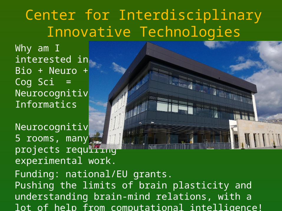
Center for InterdisciplinaryInnovative Technologies

Why am I interested in this? Bio + Neuro + Cog Sci = Neurocognitive Informatics

Neurocognitive lab,5 rooms, many projects requiring experimental work. Funding: national/EU grants. Pushing the limits of brain plasticity and understanding brain-mind relations, with a lot of help from computational intelligence!

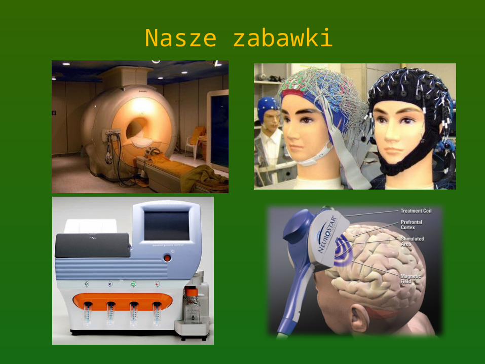
Nasze zabawki

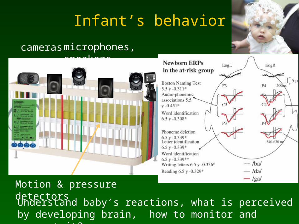
Infant’s behavior

cameras microphones, speakers

Motion & pressure detectors

Understand baby’s reactions, what is perceived by developing brain, how to monitor and correct it?

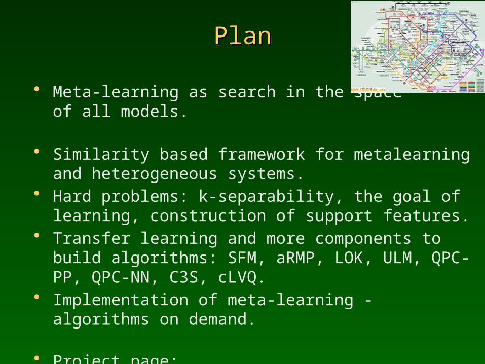
PlanPlan

• Meta-learning as search in the space of all models.

• Similarity based framework for metalearning and heterogeneous systems.

• Hard problems: k-separability, the goal of learning, construction of support features.

• Transfer learning and more components to build algorithms: SFM, aRMP, LOK, ULM, QPC-PP, QPC-NN, C3S, cLVQ.

• Implementation of meta-learning - algorithms on demand.

• Project page: http://www.is.umk.pl/projects/meta.html

What can we learn?What can we learn?

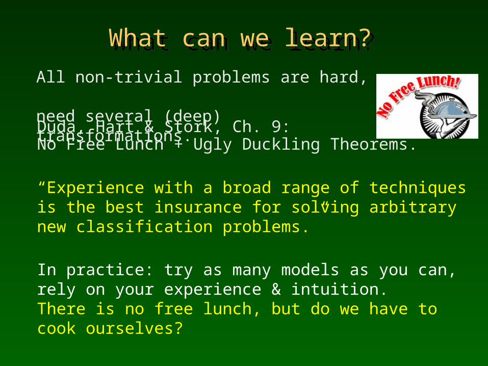
All non-trivial problems are hard, need several (deep) transformations.

Duda, Hart & Stork, Ch. 9: No Free Lunch + Ugly Duckling Theorems.

“Experience with a broad range of techniques is the best insurance for solving arbitrary new classification problems.”

In practice: try as many models as you can, rely on your experience & intuition. There is no free lunch, but do we have to cook ourselves?

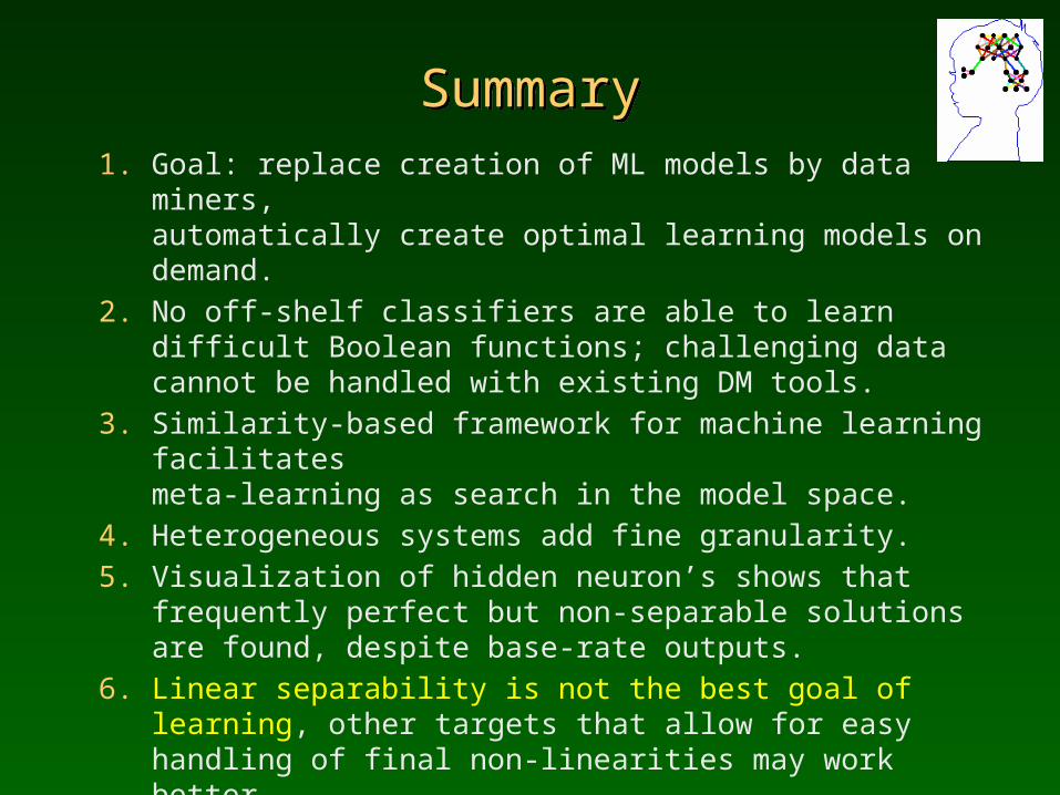
SummarySummary1. Goal: replace creation of ML models by data miners,

automatically create optimal learning models on demand.

2. No off-shelf classifiers are able to learn difficult Boolean functions; challenging data cannot be handled with existing DM tools.

3. Similarity-based framework for machine learning facilitates meta-learning as search in the model space.

4. Heterogeneous systems add fine granularity.

5. Visualization of hidden neuron’s shows that frequently perfect but non-separable solutions are found, despite base-rate outputs.

6. Linear separability is not the best goal of learning, other targets that allow for easy handling of final non-linearities may work better.

7. k-separability defines complexity classes for non-separable data.

8. Feature construction is the key element supporting learning and transfer knowledge between data models.

9. => Deep transformation-based meta-learning is needed.

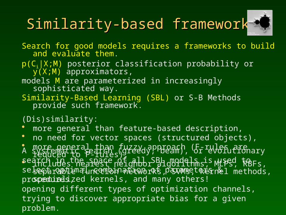
Similarity-based frameworkSimilarity-based frameworkSearch for good models requires a frameworks to build and evaluate them. p(Ci|X;M) posterior classification probability or y(X;M) approximators,models M are parameterized in increasingly sophisticated way. Similarity-Based Learning (SBL) or S-B Methods provide such framework.

(Dis)similarity: • more general than feature-based description, • no need for vector spaces (structured objects), • more general than fuzzy approach (F-rules are reduced to P-rules), • includes nearest neighbor algorithms, MLPs, RBFs, separable function

networks, SVMs, kernel methods, specialized kernels, and many others!

A systematic search (greedy, beam), or evolutionary search in the space of all SBL models is used to select optimal combination of parameters & procedures, opening different types of optimization channels, trying to discover appropriate bias for a given problem.

Result: several candidate models are created, already first very limited version gave best results in 7 out of 12 Stalog problems.

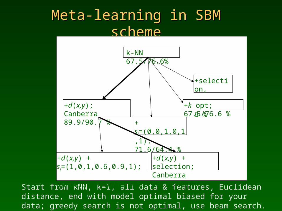
Meta-learning in SBM schemeMeta-learning in SBM scheme

Start from kNN, k=1, all data & features, Euclidean distance, end with model optimal biased for your data; greedy search is not optimal, use beam search.

k-NN 67.5/76.6%

+d(x,y); Canberra 89.9/90.7 %

+ si=(0,0,1,0,1,1); 71.6/64.4 %

+selection, 67.5/76.6 %

+k opt; 67.5/76.6 %

+d(x,y) + si=(1,0,1,0.6,0.9,1); Canberra 74.6/72.9 %

+d(x,y) + selection; Canberra 89.9/90.7 %

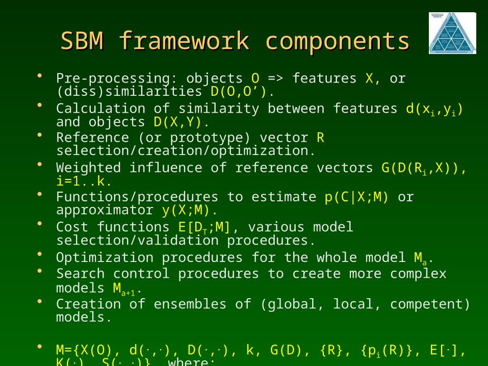
SBM framework componentsSBM framework components• Pre-processing: objects O => features X, or (diss)similarities D(O,O’). • Calculation of similarity between features d(xi,yi) and objects D(X,Y).• Reference (or prototype) vector R selection/creation/optimization. • Weighted influence of reference vectors G(D(Ri,X)), i=1..k.• Functions/procedures to estimate p(C|X;M) or approximator y(X;M). • Cost functions E[DT;M], various model selection/validation procedures. • Optimization procedures for the whole model Ma.• Search control procedures to create more complex models Ma+1.• Creation of ensembles of (global, local, competent) models.

• M={X(O), d(.,.), D(.,.), k, G(D), {R}, {pi(R)}, E[.], K(.), S(.,.)}, where:• S(Ci,Cj) is a matrix evaluating similarity of the classes;

a vector of observed probabilities pi(X) instead of hard labels.

The kNN model p(Ci|X;kNN) = p(Ci|X;k,D(.),{DT}); the RBF model: p(Ci|X;RBF) = p(Ci|X;D(.),G(D),{R}), MLP, SVM and many other models may all be “re-discovered” as a part of SBL.

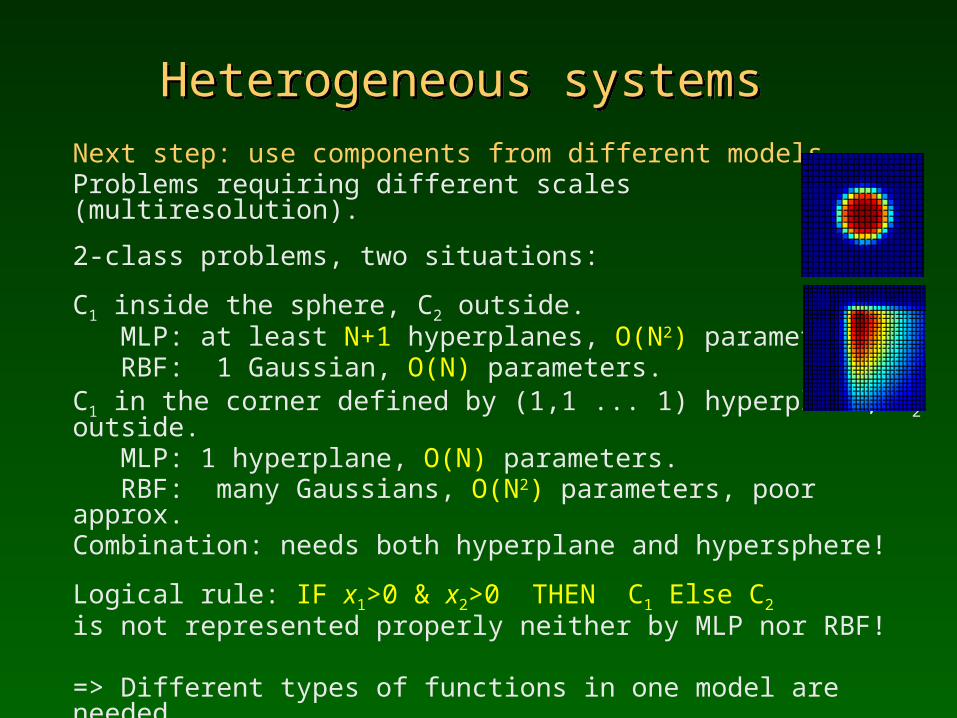
Heterogeneous systemsHeterogeneous systemsNext step: use components from different models. Problems requiring different scales (multiresolution).

2-class problems, two situations:

C1 inside the sphere, C2 outside.MLP: at least N+1 hyperplanes, O(N2) parameters. RBF: 1 Gaussian, O(N) parameters.

C1 in the corner defined by (1,1 ... 1) hyperplane, C2 outside.MLP: 1 hyperplane, O(N) parameters. RBF: many Gaussians, O(N2) parameters, poor approx.

Combination: needs both hyperplane and hypersphere!

Logical rule: IF x1>0 & x2>0 THEN C1 Else C2

is not represented properly neither by MLP nor RBF!

=> Different types of functions in one model are needed.Inspirations from single neurons => neural minicolumns, complex processing.

Heterogeneous everythingHeterogeneous everythingHomogenous systems: one type of “building blocks”, same type of decision borders, ex: neural networks, SVMs, decision trees, kNNsCommittees combine many models together, but lead to complex models that are difficult to understand.

Ockham razor: simpler systems are better. Discovering simplest class structures, inductive bias of the data, requires Heterogeneous Adaptive Systems (HAS).

HAS examples:NN with different types of neuron transfer functions.k-NN with different distance functions for each prototype.Decision Trees with different types of test criteria.

1. Start from large network, use regularization to prune.2. Construct network adding nodes selected from a candidate pool.3. Use very flexible functions, force them to specialize.

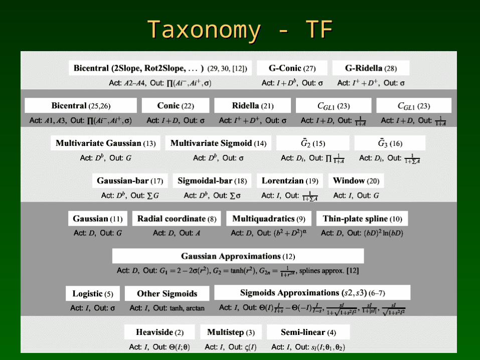
Taxonomy - TFTaxonomy - TF

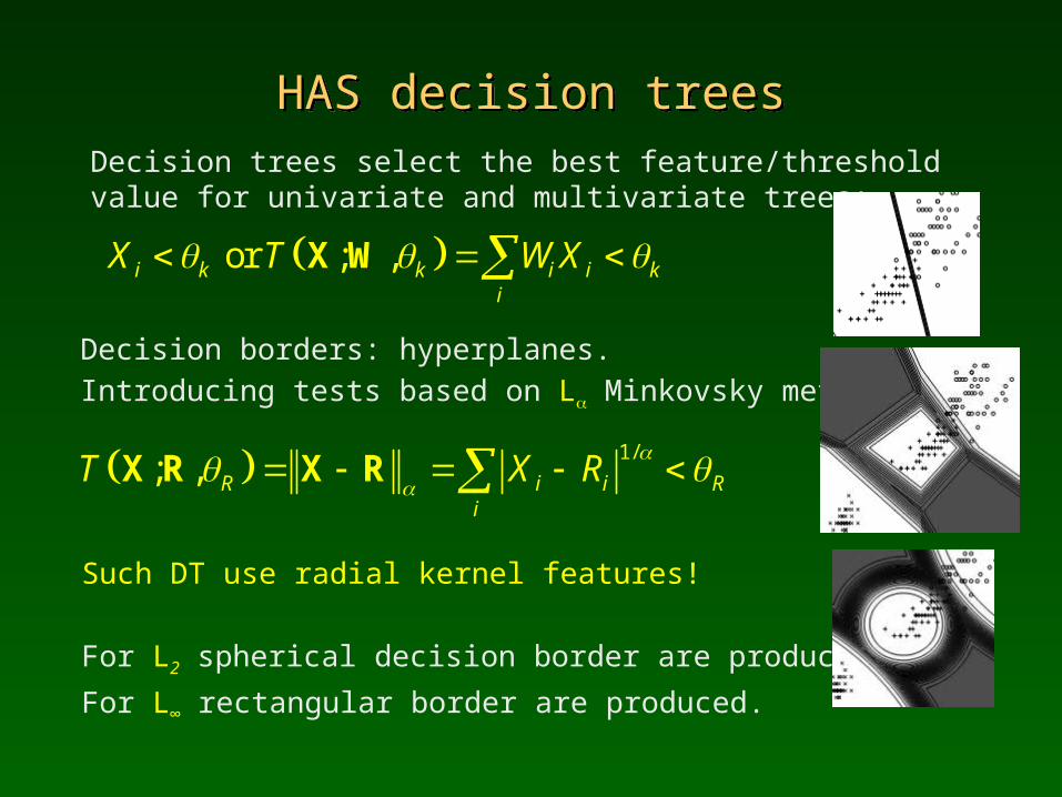
HAS decision treesHAS decision treesDecision trees select the best feature/threshold value for univariate and multivariate trees:

Decision borders: hyperplanes.

Introducing tests based on La Minkovsky metric.

or ; ,i k k i i ki

X T W X X W

Such DT use radial kernel features!

For L2 spherical decision border are produced.

For L∞ rectangular border are produced.

1/; , R i i R

i

T X R

X R X R

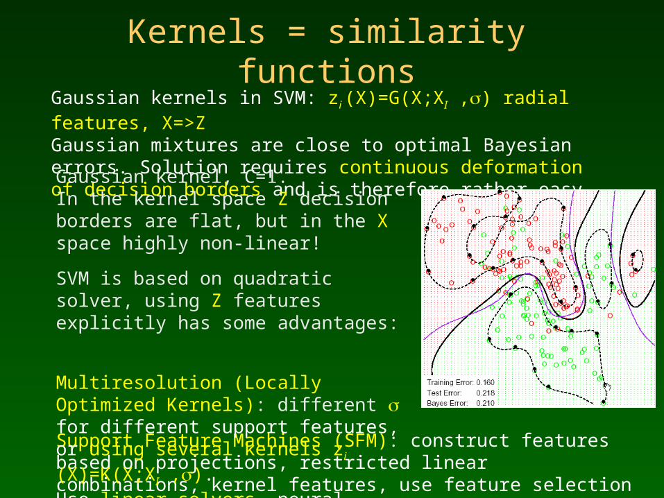
Kernels = similarity functionsGaussian kernels in SVM: zi (X)=G(X;XI ,s) radial features, X=>ZGaussian mixtures are close to optimal Bayesian errors. Solution requires continuous deformation of decision borders and is therefore rather easy.

Support Feature Machines (SFM): construct features based on projections, restricted linear combinations, kernel features, use feature selection ...

Gaussian kernel, C=1.In the kernel space Z decision borders are flat, but in the X space highly non-linear!

SVM is based on quadratic solver, using Z features explicitly has some advantages:

Multiresolution (Locally Optimized Kernels): different s for different support features, or using several kernels zi (X)=K(X;XI ,s). Use linear solvers, neural network, Naïve Bayes, or any other algorithm, all work fine.

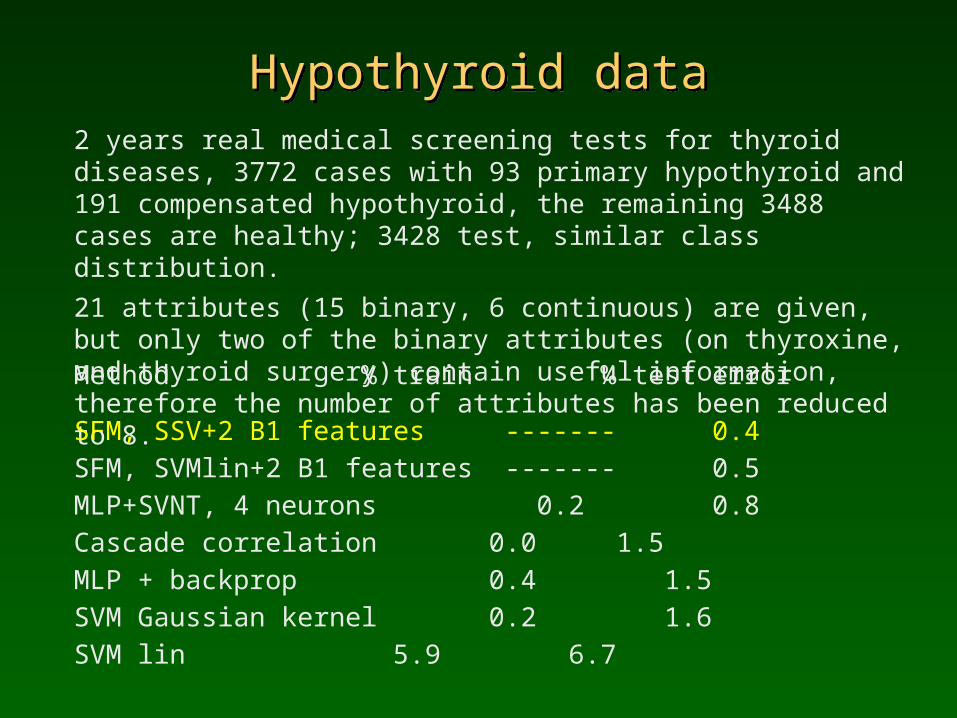
Hypothyroid dataHypothyroid data2 years real medical screening tests for thyroid diseases, 3772 cases with 93 primary hypothyroid and 191 compensated hypothyroid, the remaining 3488 cases are healthy; 3428 test, similar class distribution. 21 attributes (15 binary, 6 continuous) are given, but only two of the binary attributes (on thyroxine, and thyroid surgery) contain useful information, therefore the number of attributes has been reduced to 8.

Method % train % test error

SFM, SSV+2 B1 features ------- 0.4 SFM, SVMlin+2 B1 features ------- 0.5 MLP+SVNT, 4 neurons 0.2 0.8 Cascade correlation 0.0 1.5MLP + backprop 0.4 1.5 SVM Gaussian kernel 0.2 1.6 SVM lin 5.9 6.7

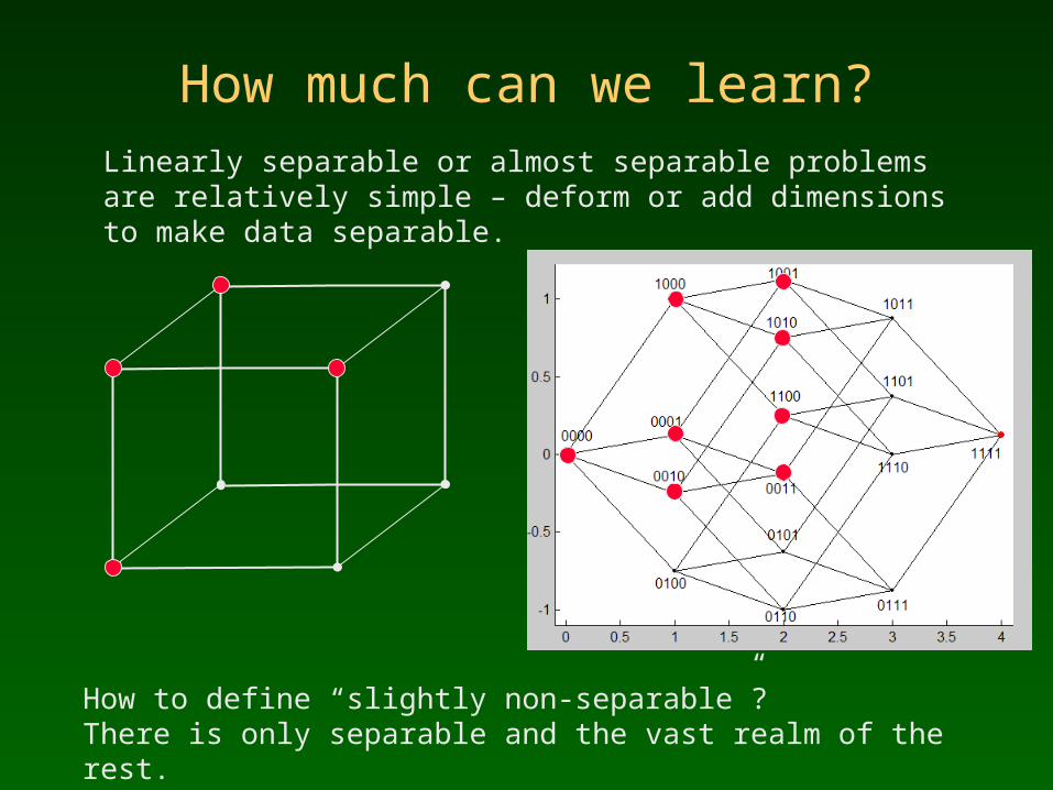
How much can we learn?Linearly separable or almost separable problems are relatively simple – deform or add dimensions to make data separable.

How to define “slightly non-separable”? There is only separable and the vast realm of the rest.

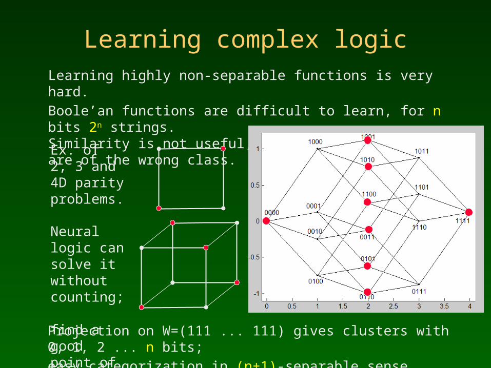
Learning complex logicLearning highly non-separable functions is very hard.

Boole’an functions are difficult to learn, for n bits 2n strings. Similarity is not useful, for parity all neighbors are of the wrong class.

Projection on W=(111 ... 111) gives clusters with 0, 1, 2 ... n bits;

easy categorization in (n+1)-separable sense.

Ex. of 2, 3 and 4D parity problems.

Neural logic can solve it without counting; find a good point of view.

Boolean functionsBoolean functionsn=2, 16 functions, 12 separable, 4 not separable.

n=3, 256 f, 104 separable (41%), 152 not separable.

n=4, 64K=65536, only 1880 separable (3%)

n=5, 4G, but << 1% separable ... bad news!

Existing methods may learn some non-separable functions, but in practice most functions cannot be learned !

Example: n-bit parity problem; many papers in top journals.

No off-the-shelf systems are able to solve such problems.

For all parity problems SVM is below base rate!

Such problems are solved only by specially designed classifiers.

Parity is trivial, solved by

1

cosn

ii

y b

Goal of learningGoal of learning

If complex logic is inherent in data models based on topological

deformation of decision borders will not be sufficient.

Exponentially large number of localized functions is required.

Linear separation is too difficult, set an easier goal for learning.

Linear separation: projection on 2 half-lines in the kernel space:

line y=WX, with y<0 for class –, and y>0 for class +.

Simplest extension that is easier to achieve:

separation into k-intervals, or k-separability.

For parity: find directions y=W.X with minimum # of pure intervals.

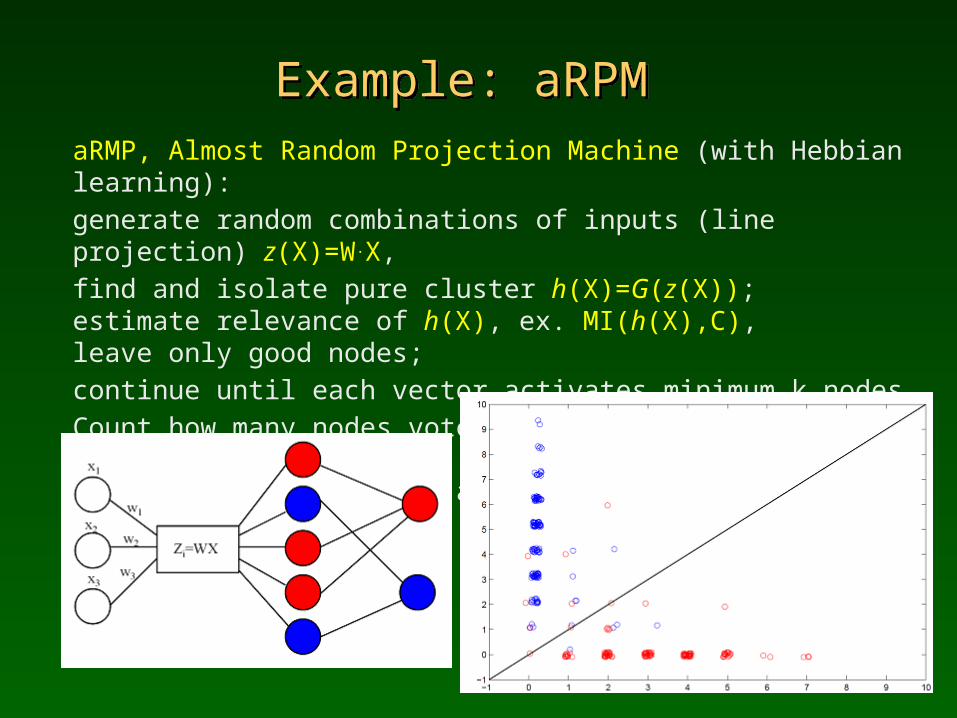
Example: aRPMExample: aRPMaRMP, Almost Random Projection Machine (with Hebbian learning): generate random combinations of inputs (line projection) z(X)=W.X, find and isolate pure cluster h(X)=G(z(X)); estimate relevance of h(X), ex. MI(h(X),C), leave only good nodes;continue until each vector activates minimum k nodes.Count how many nodes vote for each class and plot: no LDA needed! No need for learning at all!

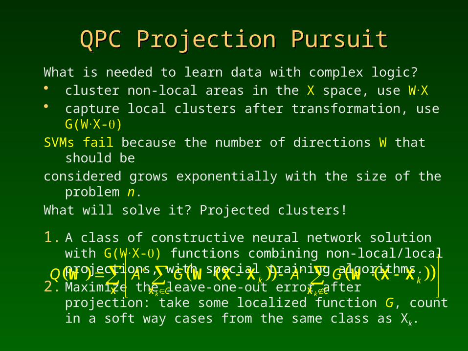
QPC Projection PursuitQPC Projection PursuitWhat is needed to learn data with complex logic?• cluster non-local areas in the X space, use W.X• capture local clusters after transformation, use G(W.X-q) SVMs fail because the number of directions W that should be considered grows exponentially with the size of the problem n.What will solve it? Projected clusters!

1. A class of constructive neural network solution with G(W.X-q) functions combining non-local/local projections, with special training algorithms.

2. Maximize the leave-one-out error after projection: take some localized function G, count in a soft way cases from the same class as Xk.

Grouping and separation; projection may be done directly to 1 or 2D for visualization, or higher D for dimensionality reduction, if W has d columns.

k k

k kC C

Q A G A G

X X X

W W X X W X X

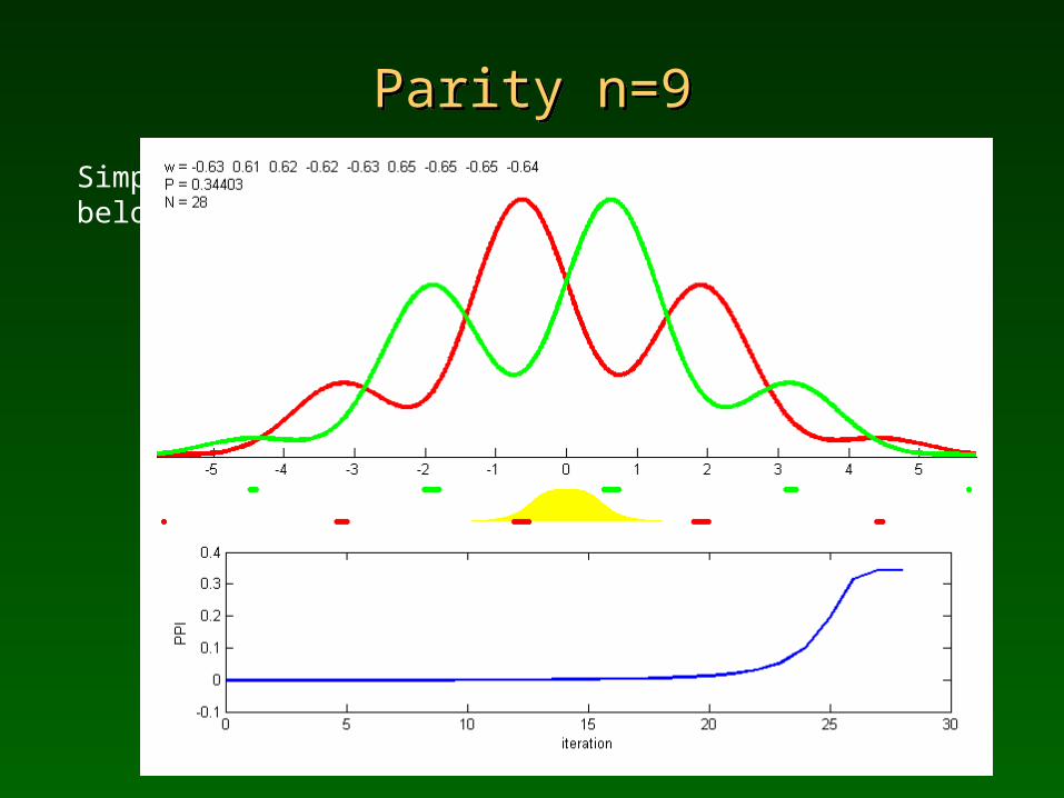
Parity n=9Parity n=9

Simple gradient learning; QCP quality index shown below.

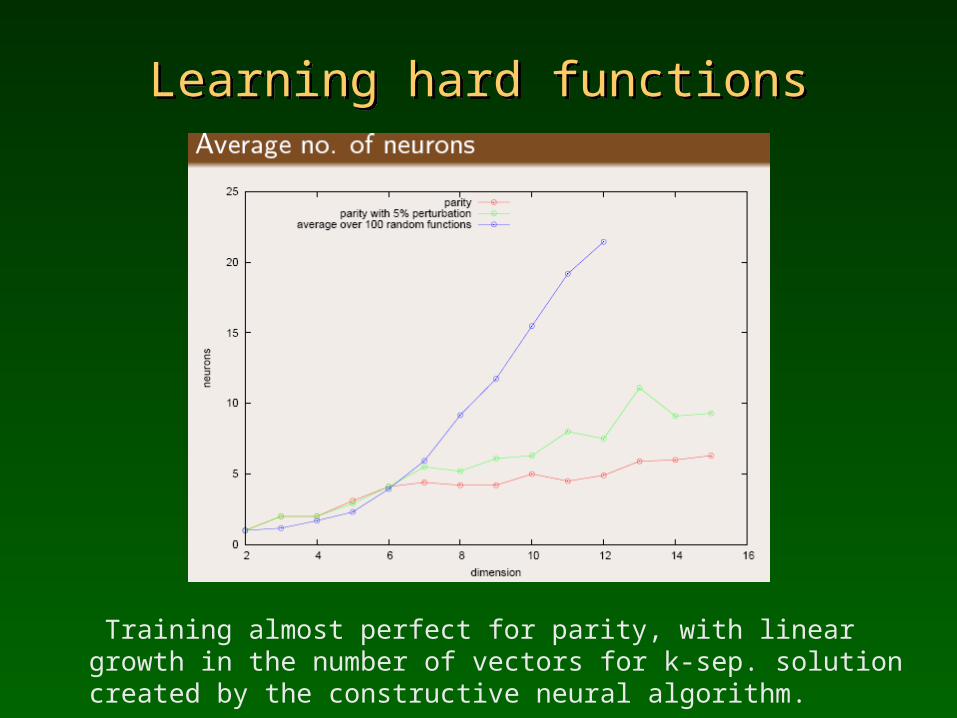
Learning hard functionsLearning hard functions

Training almost perfect for parity, with linear growth in the number of vectors for k-sep. solution created by the constructive neural algorithm.

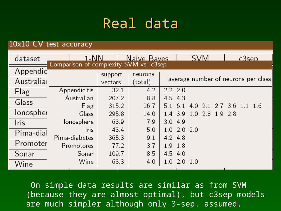
Real dataReal data

On simple data results are similar as from SVM (because they are almost optimal), but c3sep models are much simpler although only 3-sep. assumed.

Only 13 out of 45 UCI problems are non-trivial, less than 30%!Only 13 out of 45 UCI problems are non-trivial, less than 30%!

For these problems G-SVM is significantly better than O(nd) methods. For these problems G-SVM is significantly better than O(nd) methods.

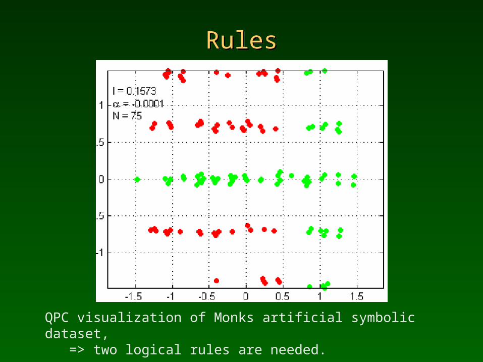
RulesRules

QPC visualization of Monks artificial symbolic dataset, => two logical rules are needed.

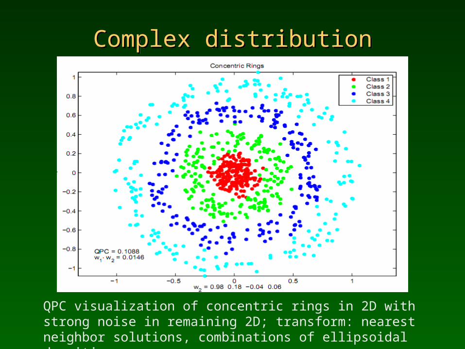
Complex distributionComplex distribution

QPC visualization of concentric rings in 2D with strong noise in remaining 2D; transform: nearest neighbor solutions, combinations of ellipsoidal densities.

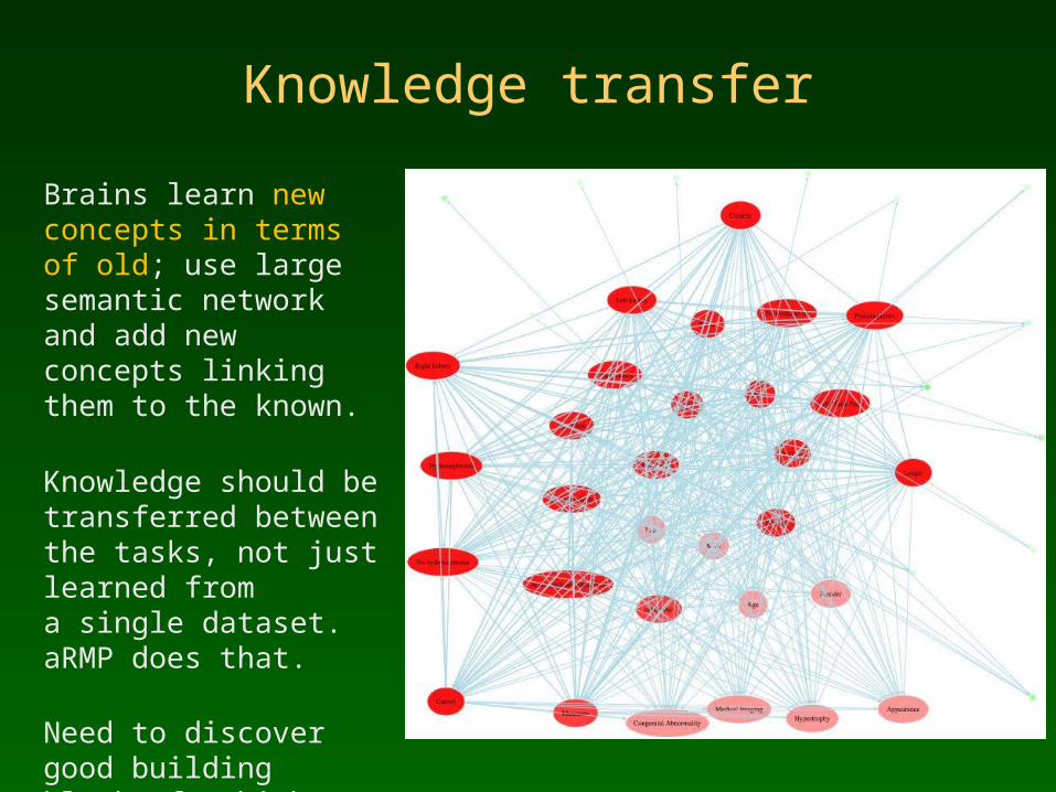
Knowledge transfer

Brains learn new concepts in terms of old; use large semantic network and add new concepts linking them to the known.

Knowledge should be transferred between the tasks, not just learned from a single dataset. aRMP does that.

Need to discover good building blocks for higher level concepts/features.

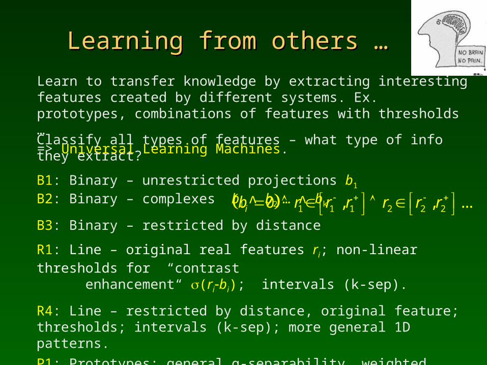
Learning from others … Learning from others …

Learn to transfer knowledge by extracting interesting features created by different systems. Ex. prototypes, combinations of features with thresholds … => Universal Learning Machines.

Classify all types of features – what type of info they extract?

B1: Binary – unrestricted projections b1 B2: Binary – complexes b1 ᴧ b2 … ᴧ bk

B3: Binary – restricted by distance

R1: Line – original real features ri; non-linear thresholds for “contrast enhancement“ s(ri-bi); intervals (k-sep).

R4: Line – restricted by distance, original feature; thresholds; intervals (k-sep); more general 1D patterns. P1: Prototypes: general q-separability, weighted distance functions or specialized kernels. M1: Motifs, based on correlations between elements rather than input values.

1 1 1 2 2 20 , , ...ib r r r r r r

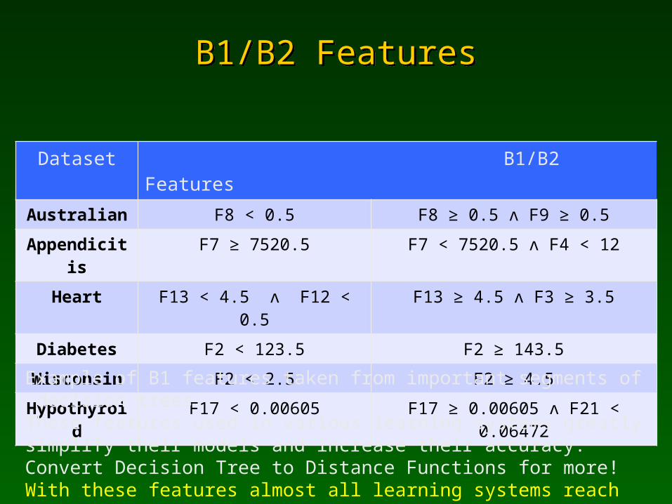
B1/B2 FeaturesB1/B2 Features

Dataset B1/B2 Features

Australian F8 < 0.5 F8 ≥ 0.5 ᴧ F9 ≥ 0.5

Appendicitis F7 ≥ 7520.5 F7 < 7520.5 ᴧ F4 < 12

Heart F13 < 4.5 ᴧ F12 < 0.5 F13 ≥ 4.5 ᴧ F3 ≥ 3.5

Diabetes F2 < 123.5 F2 ≥ 143.5

Wisconsin F2 < 2.5 F2 ≥ 4.5

Hypothyroid F17 < 0.00605 F17 ≥ 0.00605 ᴧ F21 < 0.06472

Example of B1 features taken from important segments of decision trees.These features used in various learning systems greatly simplify their models and increase their accuracy. Convert Decision Tree to Distance Functions for more!With these features almost all learning systems reach similar high accuracy!

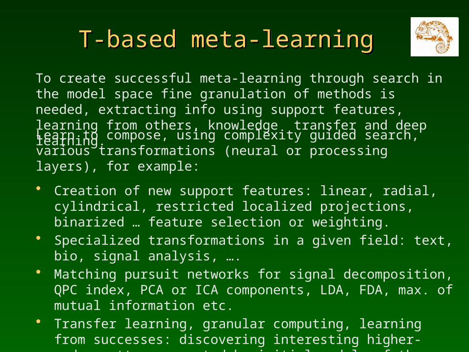
T-based meta-learningT-based meta-learning

To create successful meta-learning through search in the model space fine granulation of methods is needed, extracting info using support features, learning from others, knowledge transfer and deep learning.

Learn to compose, using complexity guided search, various transformations (neural or processing layers), for example:

• Creation of new support features: linear, radial, cylindrical, restricted localized projections, binarized … feature selection or weighting.

• Specialized transformations in a given field: text, bio, signal analysis, ….• Matching pursuit networks for signal decomposition, QPC index, PCA or ICA

components, LDA, FDA, max. of mutual information etc. • Transfer learning, granular computing, learning from successes: discovering

interesting higher-order patterns created by initial models of the data.• Stacked models: learning from the failures of other methods.• Schemes constraining search, learning from the history of previous runs at

the meta-level.

Support Feature MachinesSupport Feature Machines

General principle: complementarity of information processed by parallel interacting streams with hierarchical organization (Grossberg, 2000).Cortical minicolumns provide various features for higher processes.Create information that is easily used by various ML algorithms: explicitly build enhanced space adding more transformations.

• X , original features• Z=WX, random linear projections, other projections (PCA< ICA, PP)• Q = optimized Z using Quality of Projected Clusters or other PP techniques.• H=[Z1,Z2], intervals containing pure clusters on projections. • K=K(X,Xi), kernel features.• HK=[K1,K2], intervals on kernel features

Kernel-based SVM is equivalent to linear SVM in the explicitly constructed kernel space, enhancing this space leads to improvement of results. LDA is one option, but many other algorithms benefit from information in enhanced feature spaces; best results in various combination X+Z+Q+H+K+HK.