
arXiv:quant-ph/9910117v1 28 Oct 1999 · arXiv:quant-ph/9910117v1 28 Oct 1999 Rozprawa doktorska...
95
arXiv:quant-ph/9910117v1 28 Oct 1999 Rozprawa doktorska przygotowana w Instytucie Fizyki Teoretycznej Uniwersytetu Warszawskiego pod kierunkiem Prof. Krzysztofa W´ odkiewicza Wydzial Fizyki Uniwersytet Warszawski Warszawa 1999
Transcript of arXiv:quant-ph/9910117v1 28 Oct 1999 · arXiv:quant-ph/9910117v1 28 Oct 1999 Rozprawa doktorska...

arX
iv:q
uant
-ph/
9910
117v
1 2
8 O
ct 1
999
Rozprawa doktorska przygotowanaw Instytucie Fizyki TeoretycznejUniwersytetu Warszawskiegopod kierunkiem Prof. KrzysztofaWodkiewicza
Wydział FizykiUniwersytet Warszawski
Warszawa 1999

Contents
1 Introduction 3
2 Phase space representations of quantum state 9
2.1 Wigner function . . . . . . . . . . . . . . . . . . . . . . . . . . . . . . . . . .. 9
2.2 Quasidistribution functions . . . . . . . . . . . . . . . . . . . . . .. . . . . . . 11
2.3 Quantum interference in phase space . . . . . . . . . . . . . . . . .. . . . . . . 13
2.4 Deconvolution . . . . . . . . . . . . . . . . . . . . . . . . . . . . . . . . . . .. 15
2.5 Multimode quasidistributions . . . . . . . . . . . . . . . . . . . . .. . . . . . . 16
2.6 Quasidistribution functionals . . . . . . . . . . . . . . . . . . . .. . . . . . . . 17
3 Homodyne techniques for quantum state measurement 21
3.1 Balanced homodyne detector . . . . . . . . . . . . . . . . . . . . . . . .. . . . 22
3.2 Double homodyne detection . . . . . . . . . . . . . . . . . . . . . . . . .. . . 25
3.3 Optical homodyne tomography . . . . . . . . . . . . . . . . . . . . . . .. . . . 27
3.4 Random phase homodyne detection . . . . . . . . . . . . . . . . . . . .. . . . 30
4 Direct probing of quantum phase space 33
4.1 Wigner function and photon statistics . . . . . . . . . . . . . . .. . . . . . . . 34
4.2 Phase space picture . . . . . . . . . . . . . . . . . . . . . . . . . . . . . . .. . 36
4.3 Generalization . . . . . . . . . . . . . . . . . . . . . . . . . . . . . . . . . .. . 38
4.4 Multimode approach . . . . . . . . . . . . . . . . . . . . . . . . . . . . . . .. 40
4.5 Examples of photocount statistics . . . . . . . . . . . . . . . . . .. . . . . . . 42
5 Practical aspects 47
5.1 Photon count generating function . . . . . . . . . . . . . . . . . . .. . . . . . . 48
5.2 Statistical error . . . . . . . . . . . . . . . . . . . . . . . . . . . . . . . .. . . 48
5.3 Compensation of detector losses . . . . . . . . . . . . . . . . . . . .. . . . . . 50
5.4 Mode mismatch . . . . . . . . . . . . . . . . . . . . . . . . . . . . . . . . . . . 55
1
2 MEASURING QUANTUM STATE IN PHASE SPACE
6 Experiment 596.1 Principle . . . . . . . . . . . . . . . . . . . . . . . . . . . . . . . . . . . . . . .606.2 Setup . . . . . . . . . . . . . . . . . . . . . . . . . . . . . . . . . . . . . . . . 606.3 Results . . . . . . . . . . . . . . . . . . . . . . . . . . . . . . . . . . . . . . . . 626.4 Discussion . . . . . . . . . . . . . . . . . . . . . . . . . . . . . . . . . . . . . .63
7 Statistical uncertainty in photodetection measurements 677.1 Statistical analysis of experiment . . . . . . . . . . . . . . . . .. . . . . . . . . 697.2 Phase-insensitive detection of a light mode . . . . . . . . . .. . . . . . . . . . . 73
7.2.1 Direct photon counting . . . . . . . . . . . . . . . . . . . . . . . . . .. 747.2.2 Random phase homodyne detection . . . . . . . . . . . . . . . . . .. . 78
7.3 Consequences for quantum state measurement . . . . . . . . . .. . . . . . . . . 81
8 Conclusions 85
Bibliography 87

Chapter 1
Introduction
The development of quantum mechanics was connected with oneof the greatest conceptual leapsin theoretical physics. In order to describe properly microscopic phenomena, it was necessary toabandon the classical notion of a physical property, and to resort to a completely new formalismrepresenting microobjects. This formalism lies at the heart of quantum mechanics. It makes aclear distinction between the state of a physical system, and the performed observation. Thestate is characterized by a wave function, whose time evolution is governed by an appropriateequation of motion (e.g. the Schrodinger equation for a nonrelativistic particle). If we want torelate the state to quantities observed in an experiment, weneed to use the second element of thequantum mechanical formalism, i.e. the representation of the measuring apparatus in terms ofoperators acting on the wave function. According to the Borninterpretation, quantum mechanicsprovides probabilistic predictions concerning the behaviour of a quantum system [1]. Quantumdescription of an experiment specifies only the chance that the measurement will yield a givenoutcome. In order to verify such predictions, we need to repeat the measurement many times onidentically prepared systems, and then to compare the histogram of experimental outcomes withthe probability distribution calculated from the theory. The result of a single measurement cannotbe described in a deterministic way. This randomness seems to be a very fundamental featureof the microworld. So far, all attempts to introduce deterministic description of microscopicphenomena have failed, and experiments have ruled out wholeclasses of theories alternative toquantum mechanics.
Pictorially speaking, the click on a measuring apparatus isonly a faint shadow of the quantumstate, which stays hidden behind the scene, though being themain actor. However, one mightask if it is possible to reveal experimentally the complete information on the state of a quantumsystem. This cannot be the case if we are given only a single copy of the system. Any measure-ment consists in a certain kind of interaction between the system and the detecting apparatus.This interaction maps some properties of the measured system onto the state of the apparatus,and makes them accessible to our cognition. After the measurement, the state of the system isperturbed by the interaction with the detector, and it is no longer described by the original wave
3
4 MEASURING QUANTUM STATE IN PHASE SPACE
function. For example, observation of the position of a particle by scattering photons inevitablymodifies its momentum. The deleterious character of quantummeasurement was realized veryearly in the development of quantum mechanics, and it is closely related to the Heisenberg un-certainty principle [2]. Thus, our system can be detected only once, and we cannot gain moreinformation by repeating the measurement. One might try to circumvent this difficulty by de-signing a single measurement that would yield complete information on the quantum state. Sucha measurement would map each possible state of the system onto a different, fully distinguish-able state of the apparatus. This means that all the final states of the apparatus would have to bemutually orthogonal, even these corresponding to nonorthogonal initial states of the measuredsystem. Of course, this would violate unitarity of quantum evolution, and such a measurementdoes not exist. One could also consider cloning of quantum states, i.e. an operation that wouldgenerate two or more identical copies from a given system. Then, one could increase the amountof information by performing measurements on the reproduced copies. Such a strategy fails be-cause of the no-cloning theorem [3], which is a simple consequence of the quantum superpositionprinciple.
Nevertheless, no principles of quantum mechanics prevent us from characterizing the quan-tum state of anensembleof physical systems. By repeating the measurement many times onindividual copies, we may arrive at reliable information onthe properties of the ensemble. Theaim of quantum state measurement can be formulated in technological terms: suppose we havea machine producing identically prepared copies of a quantum system. When delivering thisoutput for some application, we should be able to provide itsspecification, which on the mostcomplete level means a full characterization of the quantumstate. Such a problem, apart frominteresting fundamental aspects, is currently of practical interest in many areas of science. Thisis due to extensive studies devoted presently to preparation, manipulation, and control of quan-tum systems. The motivation of this research is to overcome current technological limitations byexploiting fully possibilities offered by quantum mechanics. Let us mention just few examples.The yield of chemical reactions can be increased by controlling the quantum state of reactants[4]. Application of so-called squeezed states of light improves precision of interferometric mea-surements, which can be used to enhance sensitivity of gravitational wave detectors [5]. Coherentpreparation and manipulation of entangled multiparticle systems can be used to solve computa-tional problems intractable by classical computers [6]. Animportant matter in developing theseand other technologies is the possibility to gain extensiveand reliable information on the stateof quantum systems. The ultimate tool for this purpose is themeasurement of the completequantum state.
When characterizing ensembles, we usually need to take intoaccount the possibility of sta-tistical fluctuations, and to describe their state using themore general concept of the densitymatrix rather that a wave function. From the formal point of view, the task of characterizingthe quantum state can be accomplished by a set of appropriately chosen measurements, whichwould extract unambiguous information on all the elements of the density matrix. The crucial
CHAPTER 1. INTRODUCTION 5
question, however, is: how to do this in practice? The challenge of quantum state measurementhas several important aspects. The first one is design and realisation of measurement schemesthat yield complete characterization of the quantum state.Further, there is a nontrivial task ofextracting precise information on the quantum state from data collected in a realistic, imperfectexperimental setup. Finally, we have said above that expectation values of a sufficiently largeset of observables contain complete information on the density matrix. The problem is that trueexpectation values are obtained only in the limit of the infinite number of measurements. In areal laboratory we always deal withfiniteensembles, and this is our source of information on thequantum state, which we would like to use as efficiently as possible.
In quantum optics and related fields, several examples of simple quantum systems have beenthoroughly studied, including a single light mode, a trapped ion, and a diatomic molecule. A lotof interest has been paid to detection of subtle quantum statistical effects. It was therefore naturalthat the domain of quantum state measurement has grown mainly on the ground of advances inquantum optics. In 1993, the group of Michael Raymer at the University of Oregon demonstratedcomplete experimental characterization of the quantum state of a single light mode by means ofoptical homodyne tomography [7]. This seminal experiment was followed by extensive researchin the field of quantum state measurement. Over past several years, we have witnessed a seriesof beautiful experiments with various quantum systems [8].The vibrational state of a diatomicmolecule has been reconstructed from measurements of the time-dependent fluorescence spec-trum [9]. Optical homodyne tomography has been applied to reconstruct a whole gallery ofsqueezed states of light [10]. The motional state of a trapped ion has been characterized using avery sophisticated technique based on the monitoring of thefluorescence [11]. The tomographicmethod has been used to measure the transverse motional state of an atomic beam [12]. Allthese experiments were tightly connected with the rapid theoretical development of the domainof quantum state measurement. Numerous measurement schemes have been proposed and anal-ysed in detail. In particular, the role of statistical uncertainty has been discussed, and variousapproaches to reconstructing quantum state representations from experimental data have beendescribed.
The subject of this thesis is the measurement of the quantum state in the phase space. Theconcept of the phase space provides a bridge between the quantum mechanical formalism andclassical physics. Predictions of quantum mechanics have essentially statistical character. As arule, one can predict only probabilities of obtaining specific outcomes of a measurement. Sucha situation can be encountered in classical mechanics as well. For example, if we deal withan ensemble of classical systems, properties of a single copy can be defined only in statisticalterms. The state of the ensemble is characterized by a phase space distribution, which describesthe probability of occupying a given volume element by the system. One may wonder whetherthis intuitive picture of fluctuations has its counterpart in quantum physics. The answer to thisquestion is not straightforward. It is possible to convert the quantum mechanical formalisminto a form which resembles a classical statistical theory.The first phase space representation
6 MEASURING QUANTUM STATE IN PHASE SPACE
of the quantum state was introduced in 1932 by Wigner [13]. However, such a phase spacerepresentation is not unique: noncommutativity of quantumobservables leads to abundance ofquantum analogs of the phase space distribution, and none ofthem captures all the properties ofthe classical object [14]. This is a manifestation of the fact that quantum mechanics is essentiallydifferent from a classical theory. Nevertheless, quantum phase space quasidistributions containcomplete information on the quantum state. The family of quasidistribution functions providesa convenient framework for studying many quantum optical problems. It is also a useful tool invisualising quantum coherence and interference phenomena.
For a long time, quantum quasidistribution functions have been considered mainly as a quiteodd theoretical concept rather than a quantity which can be measured in a feasible experimentalscheme. This perspective changed completely with the demonstration of optical homodyne to-mography, which brought quasidistributions, in particular the Wigner function, to the realm ofa physical laboratory. Optical homodyne tomography is based on the observation that marginaldistributions of the Wigner function of a light mode can be measured by means of homodynedetection. The inverse problem, i.e. the retrieval of the Wigner function from its projections, issimilar to the procedure used in medical imaging, where the spatial distribution of the tissue isreconstructed from absorption measured across the body. Practical implementation of the recon-struction algorithm is a rather complex and delicate matter: the back-projection transformationis singular, and its application to experimental data has tobe accompanied by a special filteringprocedure. Demonstration of optical homodyne tomography was a successful combination of aprecise quantum optical measurement with sophisticated data processing.
In this work we develop a novel, entirely different approachto measuring quasidistributionfunctions of light. We exploit the fact that the value of a quasidistribution at a given point of thephase space is itself a well defined quantum observable. Motivated by this representation, wepropose and demonstrate an optical scheme for measuringdirectly quasidistribution functions.This method, based on photon counting, avoids the detour viacomplex numerical reconstructionalgorithm. The basic elements of our measurement scheme arevery simple. The light modewhose quantum state we want to measure is interfered with an auxiliary coherent probe field, anda photon counting detector is used to measure the photocountstatistics of the superposed fields.We show that a simple arithmetic operation performed on the measured photocount statisticsyields directly the value of the quasidistribution at a point defined by the amplitude and the phaseof the probe field. By changing these two parameters of the probe field, we may scan the completephase space, and obtain the full representation of the quantum state of the measured light mode.We demonstrate an experimental realisation of this scheme,and present measurements of theWigner function for several quantum states of light. The experimental part of this thesis hasbeen performed in Division of Optics, Institute of Experimental Physics, Warsaw University, incollaboration with Prof. Czesław Radzewicz.
We shall study here in detail various aspects of the direct scheme for measuring quasidistri-bution functions. On the practical side, there is a questionabout the role of typical experimental

CHAPTER 1. INTRODUCTION 7
imperfections. We shall analyse how the result of the measurement is affected by such factorsas non-unit detection efficiency and imperfect interference visibility. We shall also provide esti-mates for statistical error, which are necessary to design an accurate experiment, and to specifyconfidence of the experimental outcome. These theoretical results will be an important toolfor quantitative analysis of the performed experiment. In addition, our discussion of practicalaspects has interesting consequences in the recently disputed problem of compensating for de-tector losses in photodetection measurements. Over past several years, there were conflictingclaims concerning the possibility of removing deleteriouseffects of imperfect detection by ap-propriate numerical processing of experimental data [15, 16, 17]. Our measurement schemeprovides a testing ground for this problem. We will show thatin general no compensation fordetection losses is possible, unless somea priori knowledge about the measured quantum stateis given. Discussion of this problem reveals the fundamental role of statistical uncertainty inrealistic quantum measurements, which results from the fact that in a laboratory we always dealwith finite ensembles.
An attractive feature of the presented approach to measuring quasidistribution functions ofa single light mode is the direct link between the measured observable and the quantum staterepresentation. One may wonder whether this approach can beapplied in other situations. Weshall describe here a generalization of the measurement scheme to multimode radiation. We shalldemonstrate that multimode quasidistribution functions are also directly related to the photocountstatistics, and that they can be determined in an equally simple way. Although our interest in thisthesis will be confined to detection of optical radiation, itshould be noted that the idea underlyingour measurement scheme has proven to be fruitful in the measurement of the vibrational stateof a trapped ion [11]. It has also motivated measurement schemes for a cavity mode [18] and adiatomic molecule [19].
This thesis is organized as follows. In Chap. 2 we review phase space representations of thequantum state. Starting from the definition of the Wigner function, we show how this distributioncan be unified with other phase space representations, and wediscuss properties of generalizeds-ordered quasidistribution functions. In Chap. 3 we reviewbriefly previous work on measuringthe quantum state of light. We present two techniques which have been realized in experiments:optical homodyne tomography and balanced homodyne detection. Next, in Chap. 4, we intro-duce the direct method for measuring quasidistribution functions of light. We present the phasespace picture of the measurement, and we develop the multimode theory of the scheme. Variouspractical aspects of the proposed measurement are discussed in Chap. 5, including the effectsof imperfect detection, and the possibility of compensation for detector losses. In Chap. 6 wepresent experimental realization of the proposed scheme, and demonstrate the direct measure-ment of the Wigner function of a single light mode. The issue of statistical uncertainty in pho-todetection measurements is discussed from a more general point of view in Chap. 7. We showthat the statistical noise sometimes limits available information on the quantum state. Finally,Chap. 8 concludes the thesis. Major part of original resultspresented in this thesis has been

8 MEASURING QUANTUM STATE IN PHASE SPACE
published in the following articles:
• K. Banaszek and K. Wodkiewicz,Direct probing of quantum phase space by photon counting,Phys. Rev. Lett.76, 4344 (1996).
• K. Banaszek and K. WodkiewiczAccuracy of sampling quantum phase space in a photon counting experiment,J. Mod. Opt.44, 2441 (1997).
• K. Banaszek, C. Radzewicz, K. Wodkiewicz, and J. S. Krasinski,Direct measurement of the Wigner function by photon counting,Phys. Rev. A60, 674 (1999).
• K. Banaszek,Statistical uncertainty in quantum-optical photodetection measurements,J. Mod. Opt.46, 675 (1999).
Acknowledgements
First and foremost, I thank my supervisor, Prof. Krzysztof Wodkiewicz, for guiding me through-out my PhD studies, and for providing numerous comments and suggestions on drafts of thisthesis. It has been both a pleasure and a privilege to share his enthusiasm for scientific research.I am also indebted to Prof. Czesław Radzewicz and Prof. JerzyS. Krasinski, with whom I collab-orated on the experiment, for teaching me how thingsreally work. My special thanks go to Prof.Kazimierz Rzazewski and Prof. Jan Mostowski. I owe them my first encounters with quantumoptics.
Some of the results presented in this thesis were obtained during my stay in Laser Opticsand Spectroscopy Group at Imperial College, London. I wouldlike to thank the Head of theGroup, Prof. Peter L. Knight FRS, as well as all its members, for making my stay so fruitfuland enjoyable. In understanding foundations of quantum state measurement, I have benefited alot from the visit at Universita di Pavia, and collaboration with Prof. G. Mauro D’Ariano, Dr.Matteo Paris, and Dr. Massimiliano Sacchi.
Finally, I would like to thank the Foundation for Polish Science for the Domestic Grant forYoung Scholars.
Chapter 2
Phase space representations of quantumstate
In the standard formulation of quantum mechanics, the quantum state is characterized by a vectorfrom the Hilbert space describing the physical system. The state vector is related to measurablequantities by evaluating expectation values with operators which represent observables. Thisformalism is very far from a classical, intuitive picture ofstatistical fluctuations. Nevertheless,there is a possibility to transform the standard quantum mechanical formalism into the formwhich resembles a classical statistical theory. Such a representation is particularly useful ininvestigating the classical limit of quantum mechanics. The fundamental role in this approachis played by quasidistribution functions, which can be regarded as quantum analogs of a phasespace probability distribution. However, due to noncommutativity of quantum observables, thephase space representation of the quantum state is not unique, and it is not possible to have inquantum mechanics a phase space distribution that has all the properties of the classical one.
2.1 Wigner function
In 1932, Eugene Wigner [13] introduced a quantum analog of the classical phase space proba-bility distribution. For a particle travelling along one dimension, the Wigner function is relatedto the wave functionψ(x) through the formula:
W (q, p) =1
2π~
∫
dxψ∗(q + x/2) eipx/~ψ(q − x/2), (2.1)
and it completely characterizes the quantum state. The integral ofW (q, p) overq andp is one,which follows from the normalization of the wave function. Expectation values of quantumobservables can be obtained from the Wigner function by integrating it with appropriate Wigner-Weyl expressions representing these observables [14]. Furthermore, marginals of the Wignerfunction yield quantum mechanical distributions for the position and the momentum. However,
9
10 MEASURING QUANTUM STATE IN PHASE SPACE
the Wigner function has one property which manifests that quantum mechanics is distinct from aclassical statistical theory: the Wigner function can takenegative values. We shall see later thatthis property is closely related to quantum interference phenomena.
Difficulties with defining the quantum phase space distribution have their origin in the non-commutativity of quantum observables. As the position and momentum operators do not com-mute, we cannot introduce a joint distribution of these two observables. This problem is closelyrelated to the issue of the ordering of observables, which appears when passing from classical toquantum mechanics. For example, the classical expressionqp has the following nonequivalentquantum counterparts:qp, pq, or 1
2(qp + pq). The Wigner function corresponds to a specific,
symmetric ordering of the position and momentum operators,called the Weyl ordering [20]. Wewill now transform Eq. (2.1) to the form which shows explicitly relation between the Wignerfunction and the symmetric ordering of the position and momentum operators. For this purpose,let us introduce an additional delta function and representit in an integral form:
W (q, p) =1
2π~
∫
dx∫
dy eipx/~δ(y − q − x/2)ψ∗(y)ψ(y − x)
=1
(2π~)2
∫
dx∫
dy∫
dk eipx/~ei(y−q−x/2)k/~ψ∗(y)ψ(y − x)
=1
(2π~)2
∫
dx∫
dk ei(px−kq)/~∫
dy eikx/2~ψ∗(y)eik(y−x)/~ψ(y − x). (2.2)
In the last expression, the integral overy can be written as the quantum expectation value:∫
dy eikx/2~ψ∗(y)eik(y−x)/~ψ(y − x) = 〈ψ|ei(kq−px)/~|ψ〉. (2.3)
This quantity is a function of two real parametersk andx. By differentiating overk andxwe may obtain moments of the position and momentum operators. These moments are orderedsymmetrically inq andp, which follows from the form of the exponent in Eq. (2.3). Thefunction〈ψ|ei(kq−px)/~|ψ〉 is called the Wigner-Weyl ordered characteristic functionfor the position andthe momentum. Coming back to Eq. (2.2), we finally arrive at the formula
W (q, p) =1
(2π~)2
∫
dx∫
dk ei(px−kq)/~〈ψ|ei(kq−px)/~|ψ〉 (2.4)
which shows that the Wigner function is the Fourier transform of the symmetrically orderedcharacteristic function for the position and the momentum.Eq. (2.4) can be used to evaluate theWigner function corresponding to a mixed state described bythe density matrix . In such acase, we have to replace〈ψ|ei(kq−px)/~|ψ〉 by Tr(ˆei(kq−px)/~). Equivalently, the Wigner functionof a mixed state can be obtained from a weighted sum of the Wigner functions describing thepure components of the mixed state.
For a harmonic oscillator, it is convenient to introduce a pair of dimensionless annihilationand creation operators, defined by the equations:
a =1√2(λ−1q + iλ~−1p), a† =
1√2(λ−1q − iλ~−1p) (2.5)

CHAPTER 2. PHASE SPACE REPRESENTATIONS OF QUANTUM STATE 11
whereλ is a natural length scale defined by the mass and the frequencyof the oscillator. Anal-ogously, the two real parameters of the Wigner function can be combined into a single complexargumentα = (λ−1q + iλ~−1p)/
√2. The Wigner function in this parameterization is given by
W (α) =1
π2
∫
d2ζ eζ∗α−ζα∗〈eζa†−ζ∗a〉 (2.6)
where the integration is performed over the whole complex plane and the angular brackets〈. . .〉denote the quantum expectation value. Let us note, that the normalization constant in Eq. (2.6)has changed compared to Eq. (2.4). This is because the integration measure over the phase spaceis now equal to d2α = dq dp/2~.
The physical system which we shall describe in the phase space representation, is optical ra-diation. In the standard procedure of quantization, the electromagnetic field is decomposed intoa set of independent modes. Each of these modes is characterized by a pair of creation and anni-hilation operators, which satisfy bosonic commutation relations for a harmonic oscillator. Whenonly one of the modes is excited, we may describe its quantum state using the Wigner functiondefined in Eq. (2.6). In the classical limit, the parameterα characterizes the complex amplitudeof the field, expressed in dimensionless units. We may also use the single-mode description ifour measuring apparatus is sensitive only to a selected modeof the detected radiation.
2.2 Quasidistribution functions
As it is clearly seen from Eq. (2.6), the Wigner function corresponds to the characteristic func-tion with the symmetric ordering of the creation and annihilation operators. In principle, wecould consider also other orderings, for example normal or antinormal. In the normal orderingall creation operators are placed before annihilation operators, and vice versa for the antinor-mal ordering. Thus, we could think of replacing the quantum expectation value in Eq. (2.6)by the normally ordered characteristic function〈eζa†e−ζ∗a〉, or by the antinormally ordered one〈e−ζ∗aeζa†〉. These and other possibilities can be written jointly in a very elegant way by introduc-ing an exponential factor, which defines the ordering of the creation and annihilation operators.This idea leads to the concept of more generals-parameterized quasiprobability distributions.The one-parameter family of quasidistribution functions is given by the following formula [21]:
W (α; s) =1
π2
∫
d2ζ es|ζ|2/2+ζ∗α−ζα∗
⟨
eζa†−ζ∗a
⟩
. (2.7)
The real parameters is associated with the ordering of the field bosonic operators through theexponential factorexp(s|ζ |2/2). In particular, it can which can be easily checked using theBaker-Campbell-Haussdorf formula that three valuess = 1, 0, and−1 generate the normal,symmetric and antinormal ordering, respectively.
12 MEASURING QUANTUM STATE IN PHASE SPACE
The definition given by Eq. (2.7) unifies the Wigner function with other, independently devel-oped quantum analogs of a phase space distribution. For instance, normal ordering correspondsto the so-calledP function, introduced by Glauber [22] and Sudarshan [23]. This function servesas a weight function in the diagonal coherent state representation for the density matrix:
ˆ =
∫
d2αP (α) |α〉〈α|. (2.8)
On the other hand, antinormal ordering yields the distribution known as the Husimi [24] orQfunction [25, 26], which is given by the diagonal elements ofthe density matrix in the coherentstate basis:
Q(α) =1
π〈α| ˆ|α〉. (2.9)
Properties of variouss-parameterized quasidistribution functions are quite different. Thiscan be seen using the three examples of theP function, the Wigner function, and theQ function.TheP function is highly singular for nonclassical states of light. For example, it is given byderivatives of the delta function for eigenstates of the photon number operatora†a. The Wignerfunction is well behaved for all states, but it may take negative values. Finally theQ functionis always positive definite, which follows directly from Eq.(2.9). The fact that quasidistributionfunctions with lower ordering are more regular reflects a general relation linking any two differ-ently ordered quasidistributions via convolution with a Gaussian function in the complex phasespace:
W (α; s′) =2
π(s− s′)
∫
d2β exp
(
−2|α− β|2s− s′
)
W (β; s), (2.10)
wheres > s′. Thus the lower the ordering, the smoother the quasidistribution is, and fine detailsof the function are not easily visible. The Gaussian exponent appearing in the above equationcan be formally regarded as a propagator for the diffusion equation, with the ordering parameterplaying the role of the time. Following this analogy, we may write a differential equation forquasidistribution functions corresponding to a given quantum state:
∂
∂sW (α; s) = −1
2
∂2
∂α∂α∗W (α; s). (2.11)
Let us note that the above equation differs from the standarddiffusion equation by the minussign. This difference originates from the fact, that the “diffusion” of quasidistributions followsin the direction of decreasings.
In our calculations a normally ordered representation of the quasidistribution functions willbe very useful. Introducing normal ordering of the creationand annihilation operators in Eq. (2.7)allows to perform the integral explicitly, which yields:
W (α; s) =2
π(1− s)
⟨
: exp
(
− 2
1− s(a† − α∗)(a− α)
)
:
⟩
. (2.12)
CHAPTER 2. PHASE SPACE REPRESENTATIONS OF QUANTUM STATE 13
Thus thes-ordered quasidistribution function at a complex phase space pointα is given by theexpectation value of the operator
W (α; s) =2
π(1− s): exp
(
− 2
1 − s(a† − α∗)(a− α)
)
: (2.13)
Using the operator identity [27]
: exp[(eiζ − 1)v†v] : = exp(iζv†v) (2.14)
valid for an arbitrary bosonic annihilation operatorv, we may transform Eq. (2.13) to the follow-ing expression:
W (α; s) =2
π(1− s)
(
s+ 1
s− 1
)(a†−α∗)(a−α)
. (2.15)
The operator appearing in the exponent is the displaced photon number operatorn = a†a. Usingthe standard displacement operatorD(α) = exp(αa† −α∗a), we may writeW (α; s) as [28, 29]:
W (α; s) =2
π(1− s)D(α)
(
s+ 1
s− 1
)n
D†(α)
=2
π(1− s)
∞∑
n=0
(
s+ 1
s− 1
)n
D(α)|n〉〈n|D†(α). (2.16)
The last form is simply the spectral decomposition ofW (α; s). The eigenvectors are displacedFock statesD(α)|n〉, and the corresponding eigenvalues are[(s + 1)/(s − 1)]n times the frontnormalization factor2/π(1 − s). It is instructive to see, how the properties of the quasidistri-butions are reflected by the spectrum ofW (α; s). First, let us note that fors → 1, the factor(s + 1)/(s − 1) is divergent; this corresponds to the singular character oftheP representation.For 0 < s < 1 the set of eigenvalues is unbounded; therefore, the corresponding quasidistribu-tions also may exhibit singular behaviour. The operatorW (α; s) becomes bounded fors ≤ 0,and the highest value, i.e.s = 0, corresponds to the Wigner function. Even whenW (α; s) isbounded, its eigenvalues corresponding to oddns can be negative. The highest value ofs forwhich all the eigenvalues are nonnegative iss = −1, which corresponds to theQ function.
2.3 Quantum interference in phase space
We will now discuss, using a simple example, how quantum interference phenomena are visu-alised in the phase space representation. A quantum analog of a classical field with well definedamplitude and phase is the coherent state|α0〉, defined as an eigenstate of the annihilation op-eratora|α0〉 = α0|α0〉. This equivalence originates from the fact, that full quantum theory of

14 MEASURING QUANTUM STATE IN PHASE SPACE
photodetection gives for coherent states the same predictions as semiclassical theory with quan-tized detector and classical electromagnetic fields [30]. Coherent states are represented in thephase space by Gaussians
W |α0〉(α; s) =2
π(1− s)exp
(
− 2
1 − s|α− α0|2
)
. (2.17)
Quantum mechanics allows one to combine two such classical-like state, for example|α0〉and| − α0〉 into a coherent superposition
|ψ〉 = 1√
2(1 + e−2|α0|2)(|α0〉+ | − α0〉). (2.18)
States of this type illustrate quantum coherence and interference between classical–like com-ponents, and are often called quantum optical Schrodingercats [31]. In contrast to coherentstates, they exhibit a variety of nonclassical properties [32]. The quasidistribution function of thesuperposition|ψ〉 is given by the formula
W |ψ〉(α; s) =1
π(1− s)(1 + e−2|α0|2)
[
exp
(
− 2
1 − s|α− α0|2
)
+exp
(
− 2
1 − s|α + α0|2
)
+2 exp
(
2s
1− s|α0|2
)
exp
(
− 2
1 − s|α|2
)
cos
(
4Im(α0α∗)
1− s
)]
. (2.19)
The first two terms in the square brackets describe the two coherent components. The last termresults from quantum interference between these components. It contains an oscillating factorcos[4Im(α0α
∗)/(1 − s)]. It is seen that the frequency of the oscillations grows withthe dis-tance between the coherent components. The envelope of thisoscillating term is defined by theGaussianexp[−2|α|2/(1−s)], which is centered exactly half way between the interferingstates.
Fig. 2.1 shows quasidistributions plotted for three different values of the ordering parameters. The Wigner function contains an oscillating component originating from the interference be-tween the coherent states. This component is much smaller for s = −0.1 and it is completelysmeared out in theQ function, which can hardly be distinguished from that of a statistical mix-ture of two coherent states. This is because the whole interference term is multiplied by thefactorexp[2s|α0|2/(1 − s)], which quickly tends to zero with decreasings. Let us note that thelarger is the distance between the components, the faster this factor vanishes. The decay of theinterference component can be formally viewed as a result ofdiffusion, described by Eq. (2.11).Decreasing the ordering parameters makes the whole quasidistribution blurred, and this effectis particularly deleterious to the quickly oscillating pattern.

CHAPTER 2. PHASE SPACE REPRESENTATIONS OF QUANTUM STATE 15
Figure 2.1: Quasidistributions representing the Schrodinger cat state forα0 = 3i, depicted for the orderingparameterss = 0,−0.1, and−1.
2.4 Deconvolution
We have seen, using the example of the Schrodinger cat state, that signatures of quantum inter-ference can be visible better in quasidistribution functions with higher ordering. Thus, what isinteresting, is the inversion of Eq. (2.10), i.e. deconvolution of a lower-ordered quasidistributionfunction. This task is quite difficult. Let us first note that in general the integral in Eq. (2.10) failsto converge if we takes < s′. Instead, we may use the Fourier transforms of the quasidistributionfunctions
W (ζ ; s) =
∫
d2β eζβ∗−ζ∗βW (β; s) = es|ζ|
2/2〈eζa†−ζ∗a〉. (2.20)
Transition to a higher ordered quasidistribution consistsnow simply in multiplication by an ex-ponent:
W (ζ ; s′) = e(s′−s)|ζ|2/2W (ζ ; s), (2.21)
and evaluation of the inverse Fourier transform. The complete expression ofW (α; s′) in termsof a lower ordered quasidistribution has the form:
W (α; s′) =1
π2
∫
d2ζ e(s′−s)|ζ|2/2+ζ∗α−ζα∗
∫
d2β eζβ∗−ζ∗βW (β; s). (2.22)
Anticipating for a moment the connection of the quasidistributions with experiment, let us sup-pose that we are given an experimentally determined quasidistributionW (β; s), and that we aretrying to apply the deconvolution procedure described by Eq. (2.22). Usually, values ofW (β; s)
will be affected by errors originating from statistical uncertainty and various experimental imper-fections. These errors make the deconvolution a very delicate matter. The crucial problem is thatthe Fourier transformW (ζ ; s) has to be multiplied by anexplodingfactor e(s
′−s)|ζ|2/2. Experi-mental errors ofW (β; s) can generate long, slowly decaying high-frequency components in its

16 MEASURING QUANTUM STATE IN PHASE SPACE
Fourier transform. Multiplication by an exploding exponent enormously amplifies contributionof these fluctuations, which leads to huge errors of the reconstructedW (α; s). Therefore, decon-volution of experimentally determined quasidistributions according to Eq. (2.22) is practicallyimpossible.
2.5 Multimode quasidistributions
The concept of quasidistribution functions can be generalized in a straightforward manner tomultimode radiation. In analogy to Eq. (2.7), we need to takethe symmetrically ordered multi-mode characteristic function, and to evaluate its Fourier transform with an appropriately chosenGaussian factor which defines the ordering:
W (α1, . . . , αM ; s)
=1
π2M
∫
dζ1 . . .dζM exp
(
M∑
i=1
s
2|ζi|2 + ζ∗i αi − ζiα
∗i
)⟨
exp
(
M∑
i=1
ζia†i − ζ∗i ai
)⟩
.
(2.23)
Introducing normal ordering allows one to perform the integrals, which yields an explicit nor-mally ordered representation:
W (α1, . . . , αM ; s) =
(
2
π(1− s)
)M⟨
: exp
(
− 2
1− s
M∑
i=1
(a†i − α∗i )(ai − αi)
)
:
⟩
. (2.24)
Using Eq. (2.14), we may represent the quasidistribution functions as:
W (α1, . . . , αM ; s) =
(
2
π(1− s)
)M⟨
(
s+ 1
s− 1
)
∑
M
i=1(a†
i−α∗
i)(ai−αi)
⟩
. (2.25)
The expression∑M
i=1(a†i − α∗
i )(ai − αi) appearing in the exponent is simply the phase spacedisplaced operator of thetotal number of photons. In analogy to the single-mode case, we maywrite the multimode quasidistributions as an expectation value of the operator involving themultimode displacement operator
D({αi}) = exp
(
M∑
i=1
αia†i − α∗
i ai
)
, (2.26)
and the total photon number operator, defined as
N =
M∑
i=1
ni (2.27)
CHAPTER 2. PHASE SPACE REPRESENTATIONS OF QUANTUM STATE 17
whereni = a†i ai. The explicit expressions are:
W (α1, . . . , αM ; s) =
(
2
π(1− s)
)M⟨
D({αi}) : exp(
− 2N
1− s
)
: D†({αi})⟩
=
(
2
π(1− s)
)M⟨
D({αi})(
s+ 1
s− 1
)N
D†({αi})⟩
. (2.28)
2.6 Quasidistribution functionals
The representation given in Eq. (2.28) suggests generalization of the multimode quasidistributionfunctions to the form independent of the specific decomposition into modes. Such generalizedquasidistributions are functionals of the electromagnetic field. Instead of using a finite set ofannihilation and creation operators, we will now deal with the full description of the electromag-netic field, involving the operator fieldsE(r, t) andH(r, t). In order to simplify the notation, weshall fix the timet, and omit it in the subsequent formulae. The definition of quasidistributionfunctionals involves two operators: the coherent displacement operatorD, and the operator ofthe total number of photonsN . The action of the displacement operator is straightforward: itadds a classical amplitude to the field operators according to the formula
D[E(r),H(r)]E(r)D†[E(r),H(r)] = E(r)−E(r)
D[E(r),H(r)]H(r)D†[E(r),H(r)] = H(r)−H(r). (2.29)
In order to find an explicit formula for quasidistribution functionals, we need to express the totalphoton number operatorN in terms of the electric and magnetic field. We shall start from thestandard decomposition of the electromagnetic field into plane waves with periodic boundaryconditions in a box of the volumeV :
E(r) = i∑
lσ
√
~ωl2ǫ0V
elσ(alσeiklr − a†lσe
−iklr) (2.30)
H(r) = − i
cµ0
∑
lσ
√
~ωl2ǫ0V
elσ ×kl
|kl|(alσe
iklr − a†lσe−iklr). (2.31)
Here the indicesl andσ label respectively the wave vectorskl and the polarizationselσ, andωl = c|kl| is the frequency of anlth mode. Our goal is to represent the sum
N =∑
lσ
a†lσalσ (2.32)
usingE(r) andH(r). For this purpose we shall take Fourier transforms of these fields:∫
d3r E(r)e−iklr = i
√
~ωlV
2ǫ0
∑
σ
(elσalσ − e−lσa†−lσ) (2.33)
18 MEASURING QUANTUM STATE IN PHASE SPACE
∫
d3r H(r)e−iklr = −i
√
~ωlV
2µ0
∑
σ
(
elσ ×kl
|kl|alσ − e−lσ ×
k−l
|k−l|a†−lσ
)
. (2.34)
Here on the right-hand sides we have used the fact thatk−l = −kl. The product of the Fouriertransforms taken forkl andk−l can be expressed as:∫
d3r
∫
d3r′E(r)E(r′)e−ikl(r−r′) =
~ωlV
2ǫ0
∑
σσ′
(elσalσ − e−lσa†−lσ)(elσ′ a
†lσ′ − e−lσ′ a−lσ′)
(2.35)and∫
d3r
∫
d3r′H(r)H(r′)e−ikl(r−r′)
=~ωlV
2µ0
∑
σσ′
(
elσ ×kl
|kl|alσ − e−lσ ×
k−l
|k−l|a†−lσ
)(
elσ′ ×kl
|kl|a†lσ′ − e−lσ′ ×
k−l
|k−l|a−lσ′
)
=~ωlV
2µ0
∑
σσ′
(δσσ′ alσa†lσ′ + elσe−lσ′ alσa−lσ′ + e−lσelσ′ a
†−lσa
†lσ′ + δσσ′ a
†−lσa−lσ′). (2.36)
We shall now add the expressions for the electric and magnetic fields multiplied by the factorsǫ0/2~ωlV andµ0/2~ωlV respectively. This yields:
∫
d3r
∫
d3r′(ǫ02E(r)E(r′) +
µ0
2H(r)H(r′)
) e−ikl(r−r′)
~ωlV=∑
σ
12(alσa
†lσ + a†−lσa−lσ). (2.37)
This formula is close to the standard expression for the energy of the electromagnetic field.Indeed, we could obtain it via multiplication of both the sides by~ω, and summation overl.However, we are now interested in a different quantity, namely the total number of photons, andwe need to perform the summation with the factor~ω in the denominator of the left hand side.In this way we obtain:
∑
lσ
12(alσa
†lσ + a†lσalσ) =
∫
d3r
∫
d3r′(ǫ02E(r)E(r′) +
µ0
2H(r)H(r′)
)
K(r− r′). (2.38)
In the second term of the left-hand side we have changed the summation index−l → l. Theintegral kernelK(r− r
′) appearing on the right-hand side is given by:
K(r) =∑
l
e−iklr
~ωlV. (2.39)
We shall evaluate it in the continuous limit, when the sum over l can be replaced by a three-dimensional integral over the wave vectork. In this limit, there occurs a singularity atr = 0,which is a result of the slowly decaying integrand with largek. We shall regularize the integral
CHAPTER 2. PHASE SPACE REPRESENTATIONS OF QUANTUM STATE 19
by introducing the upper cut-offkmax for the wave number. Physically, this means that we donot take into account photons with energy larger than~ckmax. The regularized kernel can beevaluated in a straightforward manner:
K(r) =1
(2π)3~c
∫
d3ke−ikr
|k| =1
(2π)2~c
∫ kmax
0
dk k∫ π
0
dϑ sin ϑ e−ik|r| cosϑ
=1
2π2~c
1− cos kmax|r|r2
. (2.40)
It is easily seen that truncation of the wave vector magnitude has removed singularity of thekernelK(r) occurring atr = 0.
On the left-hand side of Eq. (2.38), we have a symmetrically ordered product of the creationand annihilation operators1
2(alσa
†lσ + a†lσalσ). In order to obtain the total photon number oper-
ator, we need to introduce the normal ordering of the right-hand side of Eq. (2.38). Using thisexpression, we can easily define quasidistribution functionals of the electromagnetic field. Thereis a small difficulty arising from the fact that we now deal with the infinite number of degreesof freedom. In Eq. (2.24), we cannot pass to infinity with the number of modes in the normal-ization prefactor[2/π(1 − s)]M . We shall solve this difficulty by absorbing the normalizationprefactor into the functional integration measure over thefieldsE andH. Thus, we define thequasidistribution functional as:
W[E(r),H(r); s] =
⟨
D[E(r),H(r)] : exp
(
− 2N1 − s
)
: D†[E(r),H(r)]
⟩
. (2.41)
This definition can be written explicitly using the electromagnetic field operators with the helpof the derived expression for the total photon number operator as:
W[E(r),H(r); s]
=
⟨
: exp
[
− 2
1− s
∫
d3r
∫
d3r′K(r− r
′)(ǫ02[E(r)− E(r)][E(r′)− E(r′)]
+µ0
2[H(r)−H(r)][H(r′)−H(r′)]
)
]
:
⟩
. (2.42)
The integral kernel appearing in the above formula is given by Eq. (2.39).

20 MEASURING QUANTUM STATE IN PHASE SPACE

Chapter 3
Homodyne techniques for quantum statemeasurement
Over the last decade, the domain of quantum state measurement has passed a long way fromfirst theoretical proposals to well understood experimental realizations. Complete presentationof the current state of this field would require a separate book, encompassing a wide range ofexperimental techniques and concepts of data analysis. In this chapter we shall set the scene forfurther parts of the thesis by describing briefly earlier works on measuring the quantum state oflight. We shall restrict our attention to detection of optical radiation, and describe two techniqueswhich have been successfully realized in experiments: double homodyne detection and opticalhomodyne tomography.
Double homodyne detection allows one to measure theQ function of a light mode. It wasdemonstrated in 1986 by Walker and Caroll [33]. Their experiment had as a main purpose thedemonstration of a homodyne measurement near the quantum noise limit, and it later attractedattention as a complete characterization of the quantum state. As we discussed in the previouschapter, theQ function is a positive definite distribution, and it exhibits only faint traces ofquantum interference. Optical homodyne tomography was realized first by Smitheyet al. in1993 [7]. This technique is capable of measuring the Wigner function. Apparently, this factadded extra excitement to the development of homodyne tomography, as the Wigner functionis a nonclassical distribution function which may take negative values resulting from quantuminterference.
Both these techniques are based on the same experimental apparatus, namely the balancedhomodyne detector. This device provides information on phase-sensitive properties of light. Inthe quantum mechanical formalism, it performs the measurement of a family of observablescalled quadratures. We shall start this chapter with a description of the balanced homodynedetector in Sec. 3.1. The double homodyne detection scheme is discussed in Sec. 3.2. We showthat this scheme can be used to measure two noncommuting observables at the cost of introducingextra noise to the measurement. Sec. 3.3 is devoted to optical homodyne tomography. It describes
21
22 MEASURING QUANTUM STATE IN PHASE SPACE
the physical principle of the method, as well as mathematical transformations involved in theprocessing of experimental data.
3.1 Balanced homodyne detector
Standard photodetection is insensitive to phase properties of optical radiation. This is because theobserved signal depends only on the operator of the number ofphotonsn = a†a. Nevertheless,we may use a photodetector to measure phase-dependent quantities by superposing the measuredbeam with an auxiliary coherent field using a beam splitter. The auxiliary field has the name ofthelocal oscillator. When measuring such a superposition, the signal from the photodetector willbe described by an expression involving terms linear ina anda†. Thus, it carries information onthe phase properties of the measured field. This is the basic idea of homodyne detection.
In quantum optics, homodyne detection has played an important role in investigating thesqueezed states of light. These states exhibit interestingnoise properties in certain phase-de-pendent observables. More specifically, for a single light mode we may introduce a family ofquadrature observables dependent on the phaseθ:
xθ =eiθa† + e−iθa√
2. (3.1)
It is easy to check that the commutator of two quadratures corresponding to phases which differby π/2 is [xθ, xθ+π/2] = i. Consequently, variances of these two observables satisfythe un-certainty relation in the form∆xθ∆xθ+π/2 ≥ 1/2. For coherent states, this variance is evenlydistributed over all the quadratures, and it equals to∆xθ = 1/
√2. Squeezed states are such
states of the electromagnetic field, which for a certain phaseθ have the variance smaller than thecoherent state level. These states cannot be described within classical theory of radiation, andthe squeezing is clearly a non-classical property. Squeezed states can find application in veryprecise interferometric measurements [5].
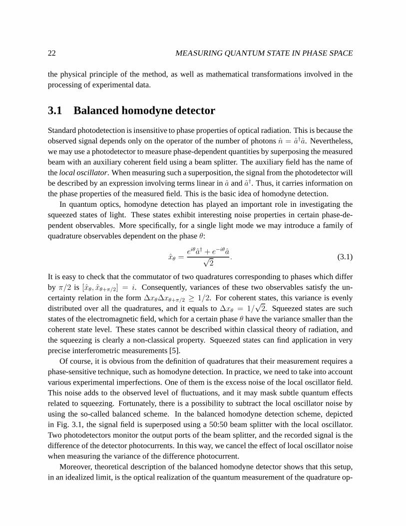
Of course, it is obvious from the definition of quadratures that their measurement requires aphase-sensitive technique, such as homodyne detection. Inpractice, we need to take into accountvarious experimental imperfections. One of them is the excess noise of the local oscillator field.This noise adds to the observed level of fluctuations, and it may mask subtle quantum effectsrelated to squeezing. Fortunately, there is a possibility to subtract the local oscillator noise byusing the so-called balanced scheme. In the balanced homodyne detection scheme, depictedin Fig. 3.1, the signal field is superposed using a 50:50 beam splitter with the local oscillator.Two photodetectors monitor the output ports of the beam splitter, and the recorded signal is thedifference of the detector photocurrents. In this way, we cancel the effect of local oscillator noisewhen measuring the variance of the difference photocurrent.
Moreover, theoretical description of the balanced homodyne detector shows that this setup,in an idealized limit, is the optical realization of the quantum measurement of the quadrature op-
CHAPTER 3. HOMODYNE TECHNIQUES. . . 23
−
50:50
ρ
|β〉LO
Figure 3.1: The balanced homodyne setup. The signal field, described by a density matrixρ, is combinedwith a coherent local oscillator|β〉LO. The two outgoing fields are measured using photodetectors.Thedifference of their counts is the statistical data recordedin the experiment.
eratorxθ. The idealization is based on two assumptions: the unit efficiency of the photodetectorsand the classical limit of the local oscillator. The latter condition can be easily satisfied in anexperiment. Also, efficiency of photodetectors used in a homodyne setup can be close to 100%.If we rely on these two assumptions, theoretical analysis ofthe balanced scheme becomes quitecompact. More detailed studies can be found in Ref. [34, 35, 36].
Let us describe the signal field with the annihilation operator a, and the local oscillator fieldwith b. These two fields, superposed on a 50:50 beam splitter, yieldtwo outgoing modes. Ingeneral, combination of the modes at a beam splitter is givenby an SU(2) transformation [37].For a 50:50 beam splitter, we may simplify this transformation to the matrix
(
c
d
)
=1√2
(
1 11 −1
)(
a
b
)
, (3.2)
wherec and d are the annihilation operators of the outgoing fields. We assume that the localoscillator is in a coherent state|β〉LO, and the quantum state of the modea is given by thedensity matrixˆ.
The quantity we are interested in is the difference of photocurrents generated by the detectorsmonitoring the modesc andd. On the microscopic level, these photocurrents consist of adiscretenumber of electronsn1 andn2. In a real experiment, this discreteness is not observed dueto thelarge average number of the generated photoelectrons. The observable measured in balanced

24 MEASURING QUANTUM STATE IN PHASE SPACE
homodyne detection is the difference of the electron number∆N = n1 − n2. The probabilityp(∆N) of obtaining a specific value for∆N can be easily derived using the standard theory ofphotoelectric detection. It is given by the expression:
p(∆N) =∑
n1−n2=∆N
Tr{ ˆ⊗ |β〉〈β|LO : e−c†c (c
†c)n1
n1!e−d
†d (d†d)n2
n2!:}. (3.3)
In further calculations, it is more convenient to deal with the generating function for the probabil-ity distributionp(∆N). The generating function is obtained by evaluating the Fourier transform:
Z(ξ) =
∞∑
∆N=−∞
eiξ∆Np(∆N)
= Tr{ ˆ⊗ |β〉〈β|LO : exp[(eiξ − 1)c†c+ (e−iξ − 1)d†d] : }. (3.4)
In this way, we managed to get rid of the troublesome constrained sum with the conditionn1 −n2 = ∆N . We can now remove the normal ordering symbol by making use ofthe operatoridentity given in Eq. (2.14). This yields:
Z(ξ) = Tr{ ˆ⊗ |β〉〈β|LO eiξ(c†c−d†d)} = Tr{ ˆ⊗ |β〉〈β|LO eiξ(a
†b+ab†)}. (3.5)
When the local oscillator is in a strong coherent state, the bosonic operatorsb, b† in the exponenteiξ(a
† b+ab†) can be replaced byc-numbersβ, β∗. In this regime, it is also convenient to rescalethe difference photocurrent∆N , which grows as the first power of the local oscillator amplitude.Dividing ∆N by |β|, we obtain a quantity which is independent of the magnitude|β| in theregime of the classical local oscillator. We shall introduce an extra factor of1/
√2, and define
the homodyne variable asx = ∆N/√2|β|. This variable can be treated as a continuous one, as
the local oscillator amplitude is very large. The rescalingof the homodyne variable correspondsto changing the parameter of the generating function according to λ = ξ
√2|β|. In the new
parameterization, the generating function takes the form:
Zθ(λ) =
⟨
exp
(
iλ√2(eiθa† + e−iθa)
)⟩
= 〈eiλxθ〉, (3.6)
whereθ is the phase of the local oscillator:β = |β|eiθ. We have added here a subscriptθ to thegenerating functionZθ(λ) to stress that the measured observable depends on the local oscillatorphase. Using the last form of theZθ(λ), we may easily obtain the probability distributionpθ(x)for the homodyne variablex by evaluating the inverse Fourier transform. Let us note that weshould now integrate over all real valuesλ because of the introduced rescaling. The inverseFourier transform yields:
pθ(x) =1
2π
∫ ∞
−∞
dλ e−iλx〈eiλxθ〉 = 〈δ(x− xθ)〉 = 〈|x〉θ θ〈x|〉 . (3.7)
This expression clearly shows, that balanced homodyne detection is the measurement of thequadrature operatorxθ. The probability of obtaining the resultx is given by the projection on thecorresponding eigenstate of the quadrature operator, defined asxθ|x〉θ = x|x〉θ.

CHAPTER 3. HOMODYNE TECHNIQUES. . . 25
3.2 Double homodyne detection
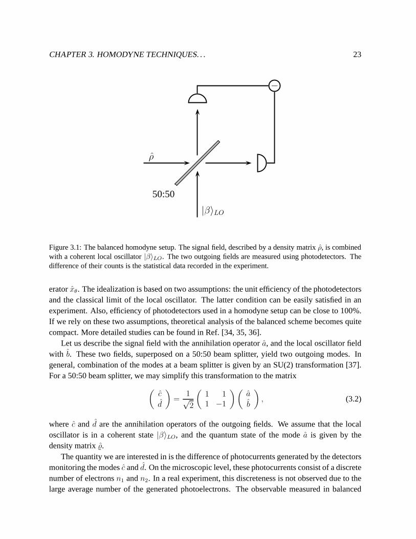
In homodyne detection, we have to select the phase of the local oscillator, which defines the mea-sured quadrature. Simultaneous measurement of different quadratures is not possible, becausethey correspond to noncommuting observables: it is easy to check that for example[xθ, xθ+π/2] =i. However, we may try to circumvent this difficulty by splitting first the input beam on a 50:50beam splitter and performingtwo homodyne measurements on the outgoing fields. This is theidea of double homodyne detection. The corresponding setupis shown in Fig. 3.2. The signalfield, described by an annihilation operatora, is divided using the 50:50 beam splitter BS. Thetwo outgoing beams are measured with two separate balanced homodyne detectors. The phasesof local oscillators can be independently adjusted in each of the arms of the setup, which allowsone to measure two arbitrary quadratures of the fields leaving the beam splitter BS. For simplic-ity, let us choose the two local oscillator phases to be0 andπ/2, and to denote the correspondingquadratures byq = x0 and p = xπ/2. These two quantities commute to the imaginary unit[q, p] = i, and they are optical analogs of the position and the momentum operators for a particle.
In the quantum description of the setup, we need to take into account the vacuum field enter-ing through the unused input port of the beam splitter BS dividing the signal field. This vacuumfield is denoted with the annihilation operatorv in Fig. 3.2. The quadratures measured at the twohomodyne detectors are given by the combinations
q1 =1√2(qa + qv), p2 =
1√2(pa − pv) (3.8)
where the indicesa andv denote quadrature operators corresponding the signal and the vacuummode respectively. The form of these combinations follows directly from Eq. (3.2), describingtransformation of the field operators at a 50:50 beam splitter.
The probability distributionp(q1, p2) for the outcomes of the measurement is now definedon the two-dimensional space spanned by the variablesq1 andp2. Analogously to the previoussection, it will be more convenient to use the generating functionZ(λ1, λ2), which depends nowon two parametersλ1 andλ2:
Z(λ1, λ2) =
∫
dλ1
∫
dλ2 eiλ1q1+iλ2q2p(q1, p2). (3.9)
The generating function describing the joint measurement of the quadraturesq1 andp2 is givenby a straightforward generalization of Eq. (3.6):
Z(λ1, λ2) = 〈exp(iλ1q1 + iλ2p2)〉a,v= exp
(
−1
8(λ21 + λ22)
)⟨
exp
(
i√2(λ1qa + λ2pa)
)⟩
a
. (3.10)
In the second line we have evaluated explicitly the quantum expectation value over the vacuummode. The joint probability distributionp(q1, p2) can be obtained from the double inverse Fourier
26 MEASURING QUANTUM STATE IN PHASE SPACE
BS
localoscillator
fields
a
v
−
−
Figure 3.2: Double homodyne detection setup. The signal field, denoted by the annihilation operatora, isdivided using a 50:50 beam splitter BS. The two outgoing fields fall onto balanced homodyne detectors.The local oscillator phases are adjusted such that two conjugate quadratures are measured. In the quantummechanical description of the setup, one has to take into account the vacuum fieldv entering through theunused input port of the beam splitter BS.
transform of the generating function. We shall rearrange this expression to the form:
p(q1, p2) =1
(2π)2
∫
dλ1
∫
dλ2 e−iλ1q1−iλ2p2Z(λ1, λ2)
=1
π2
∫
d2ζ e−|ζ|2/2+ζ∗(q1+ip2)−ζ(q1−ip2)〈eζa†−ζ∗a〉a (3.11)
where we have substitutedζ = (iλ1 − λ2)/2. The last expression can be directly related to thedefinition of quasidistribution functions in Eq. (2.7), with α = q1 + ip2, ands = −1. Thus,the joint probability distribution of homodyne events measured in double homodyne detection isequal to theQ function of the modea:
p(q1, p2) = Qa(q1 + ip2). (3.12)
One may wonder how this formula changes when we inject an arbitrary state in the secondinput port of the beam splitter BS dividing the signal field. In this caseZ(λ1, λ2) can be factorized
CHAPTER 3. HOMODYNE TECHNIQUES. . . 27
to the product of the symmetrically ordered characteristicfunctions for the position and themomentum:
Z(λ1, λ2) =
⟨
exp
(
i√2(λ1qa + λ2pa)
)⟩
a
⟨
exp
(
i√2(λ1qv + λ2pv)
)⟩
v
. (3.13)
The inverse Fourier transform maps the product of the symmetrically ordered characteristic func-tions onto a convolution of the corresponding Wigner functions. After a simple calculation, weobtain:
p(q1, p2) = 2
∫
dq∫
dpWa(q, p)Wv(√2q1 − q,
√2p2 − p), (3.14)
whereWa(q, p) andWv(q, p) are the Wigner functions describing the quantum state of thefieldsincident on the beam splitter BS.
The above results illustrates the operational approach to the joint measurement of the positionand the momentum [38, 39]. These two observables do not commute and they cannot be mea-sured simultaneously. Nevertheless, we may introduce an auxiliary system, called the “quantumruler”, and measure two commuting combinations of positions and momenta. Such a pair ofcombinations has been defined in Eq. (3.8). These two operational observables can be detectedsimultaneously, and their measurement yields a joint two-dimensional probability distribution oftwo variables which can be related to the position and the momentum. The resulting operationalphase space distribution is given by a convolution of the Wigner functions of the measured sys-tem and the ruler. Double homodyne detection is an optical realisation of this approach, withthe role of the quantum ruler played by the vacuum field. The vacuum field is described by thegaussian Wigner function, and the double homodyne detection yields a smeared Wigner functionof the signal field, which coincides with theQ function.
Double homodyne detection has been realized experimentally by Walker and Caroll [33].A thorough discussion of this technique can be found in the article by Walker [40]. The sameexperimental scheme has been applied in the operational measurement of the quantum phase[41], and it was shown later that the phase distribution measured in this scheme corresponds tothe radially integratedQ function [42, 43].
3.3 Optical homodyne tomography
In contrast to theQ function, the Wigner function does not have the operationalmeaning of aprobability distribution, simply because it may take negative values. Therefore, one cannot de-sign an experiment, in which the joint statistics of two realvariables would be described by theWigner function. Nevertheless, one-dimensional projections of the Wigner function are posi-tive definite. Furthermore, these projections describe quadrature distributions according to theformula:
pθ(x) =
∫
dyW (x cos θ − y sin θ, x sin θ + y cos θ). (3.15)
28 MEASURING QUANTUM STATE IN PHASE SPACE
p
q
W (q, p)
θ
xpθ(x)
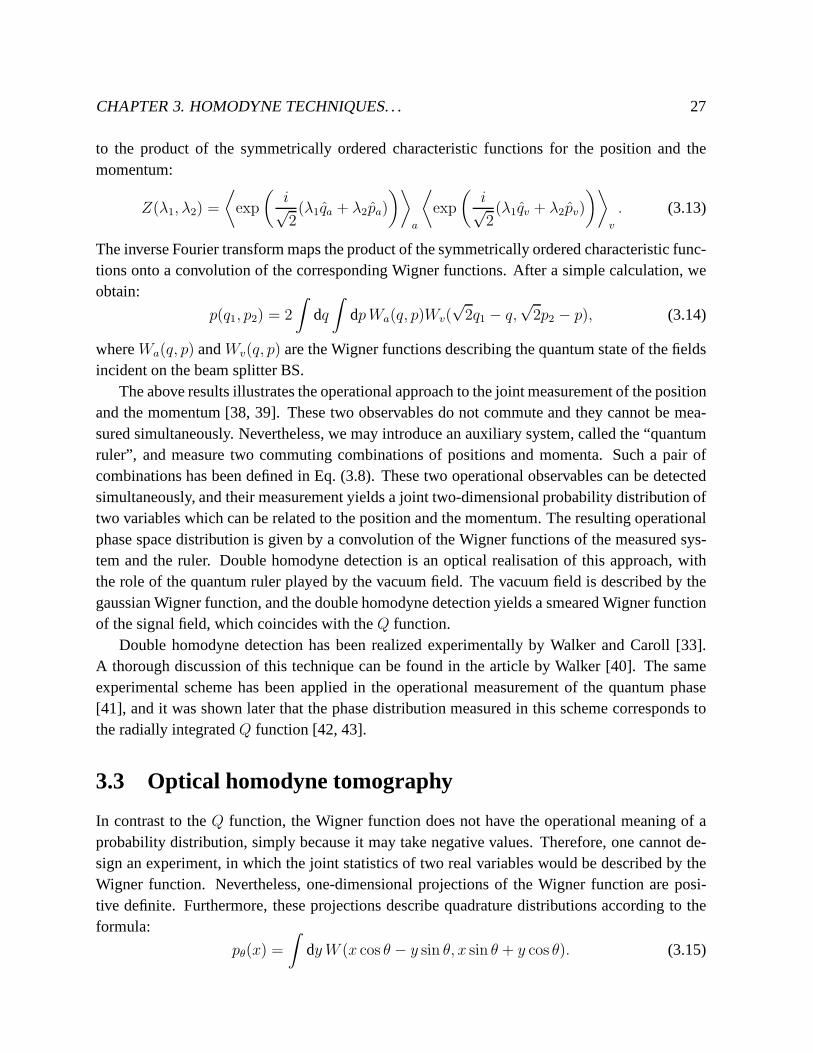
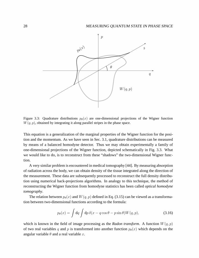
Figure 3.3: Quadrature distributionspθ(x) are one-dimensional projections of the Wigner functionW (q, p), obtained by integrating it along parallel stripes in the phase space.
This equation is a generalization of the marginal properties of the Wigner function for the posi-tion and the momentum. As we have seen in Sec. 3.1, quadraturedistributions can be measuredby means of a balanced homodyne detector. Thus we may obtain experimentally a family ofone-dimensional projections of the Wigner function, depicted schematically in Fig. 3.3. Whatwe would like to do, is to reconstruct from these “shadows” the two-dimensional Wigner func-tion.
A very similar problem is encountered in medical tomography[44]. By measuring absorptionof radiation across the body, we can obtain density of the tissue integrated along the direction ofthe measurement. These data are subsequently processed to reconstruct the full density distribu-tion using numerical back-projections algorithms. In analogy to this technique, the method ofreconstructing the Wigner function from homodyne statistics has been calledoptical homodynetomography.
The relation betweenpθ(x) andW (q, p) defined in Eq. (3.15) can be viewed as a transforma-tion between two-dimensional functions according to the formula:
pθ(x) =
∫
dq∫
dp δ(x− q cos θ − p sin θ)W (q, p), (3.16)
which is known in the field of image processing as theRadon transform. A functionW (q, p)
of two real variablesq andp is transformed into another functionpθ(x) which depends on theangular variableθ and a real variablex.
CHAPTER 3. HOMODYNE TECHNIQUES. . . 29
Inversion of the relation between the Wigner function and quadrature distributions becomesquite obvious, if we rewrite Eq. (3.15) in terms of the Fourier transforms of both the sides. Thegenerating function for the quadrature distribution can beexpressed using the Wigner functionas:
Zθ(λ) =
∫
dx eiλxpθ(x)
=
∫
dx∫
dy eiλxW (x cos θ − y sin θ, x sin θ + y cos θ)
=
∫
dq∫
dp eiλ(q cos θ+p sin θ)W (q, p). (3.17)
The last expression is simply the Fourier transform of the Wigner function taken at the point(q cos θ, p sin θ). Thus, the projection relation expressed in terms of the Fourier transforms con-sists in the change of the coordinate system, from the Cartesian one (Wigner function) to thepolar one (quadrature distributions).
With this observation in hand, the way to invert Eq. (3.15) isstraightforward: we need to writethe Wigner function as the inverse Fourier transform, and tochange the integration variables fromCartesian to polar. This allows us to insert the generating function for quadrature distributions:
W (q, p) =1
(2π)2
∫ ∞
−∞
|λ|dλ∫ π
0
dθ e−iqλ cos θ−ipλ sin θZθ(λ). (3.18)
ExpressingZθ(λ) in terms of quadrature distributions and performing the integral overλ yields:
W (q, p) =1
2π2
∫ ∞
−∞
dx∫ π
0
dθ pθ(x)d
dxP
1
x− q cos θ − p sin θ(3.19)
whereP denotes the principal value. The above formula is known asthe inverse Radon trans-form. It is clearly seen that this transformation is singular. Therefore, its numerical implementa-tion is quite complicated. When processing experimental distributionspθ(x), which are affectedby statistical noise, one has to apply a regularization scheme.
The close link between the quadrature distributions and theWigner function could be notedalready during the discussion of the balanced homodyne detector. The first expression forZθ(λ)in Eq. (3.6) is exactly the symmetrically ordered characteristic function that appears in Eq. (2.6),with ζ = iλeiθ/
√2.
The first experimental realization of optical homodyne tomography has been demonstratedby Smitheyet al. [7]. This seminal work has been followed by extensive theoretical and ex-perimental research. The effects of imperfect detection were analysed [45], and it was shownthat in such a case the inverse Radon transform yields a generalized quasidistribution functionwith the ordering parameter equal to−(1− η)/η, whereη is the efficiency of the photodetectors.Thus, detector losses result in blurring of the measured Wigner function. A more fundamental

30 MEASURING QUANTUM STATE IN PHASE SPACE
problem related to optical homodyne tomography was the determination of other quantum staterepresentations from homodyne statistics. In principle, once we have the Wigner function, wecan evaluate the expectation value of any quantum observable O, and obtain for example thedensity matrix in the Fock basis. However, it would be appealing to reconstruct the observablesdirectly from the homodyne statistics, in order to avoid thedetour via the singular inverse Radontransform. The formula needed for this purpose is of the form:
〈O〉 =∫ ∞
−∞
dx∫ π
0
dθ fO(x, θ)pθ(x), (3.20)
wherefO(x, θ) is called thepattern functionrelated to the observableO. The problem of derivingpattern functions for the elements of the density matrix in the Fock basis was studied first byD’Ariano et al. [46]. It was later generalized to a more fundamental form [47, 48]. The statisticalerror of optical homodyne tomography has been thoroughly studied in a series of papers [49, 50,51, 52]. On the experimental side, optical homodyne tomography has been demonstrated forcw fields [53], and a beautiful gallery of squeezed states of light has been presented [10]. Ananalogous tomographic method has been used to characterizetransversal degrees of freedom ofa laser beam [54].
3.4 Random phase homodyne detection
In the context of optical homodyne tomography, a new technique for measuring light has beendeveloped. This technique is balanced homodyne detection with the phaseθ made a uniformlydistributed random variable [55]. The distribution of events pR(x) observed in such a case isdescribed by phase-averaged homodyne statistics:
pR(x) =1
2π
∫ 2π
0
dθ pθ(x) =1
2π
∫ 2π
0
dθ 〈|x〉θ θ〈x|〉 . (3.21)
In this regime, the phase sensitivity of homodyne detectionis completely lost, and the phase-averaged homodyne statisticspR(x) contains information only on phase-independent propertiesof the measured light. Nevertheless, random phase homodynedetection has some advantagescompared to direct photodetection. First, ultrafast sampling time can be achieved by using thelocal oscillator field in the form of a short pulse. Second, information on the photon distributionis carried by two rather intense fields, which can be detectedwith substantially higher efficiencythan the signal field itself. This feature has enabled an experimental demonstration of even-oddoscillations in the photon distribution of the squeezed vacuum state [56].
Let us now see, how the phase-averaged homodyne statistics depends on the photon distribu-tion. We shall use the fact that eigenvectors of the quadrature operatorxθ can be obtained fromthe position eigenvectors|x〉 by the unitary transformation|x〉θ = eiθa
†a|x〉. This unitary trans-formation is diagonal in the Fock basis, andeiθa
†a|n〉 = einθ|n〉. Introducing two decompositions

CHAPTER 3. HOMODYNE TECHNIQUES. . . 31
of the identity operator in the Fock basis, we have:
pR(x) =1
2π
∫ 2π
0
dθ∞∑
m,n=0
〈|m〉〈m|x〉θ θ〈x|n〉〈n|〉
=
∞∑
m,n=0
〈m|x〉〈x|n〉∫ 2π
0
dθ2πei(n−m)θ〈|m〉〈n|〉
=∞∑
m=0
|〈m|x〉|2〈|m〉〈m|〉 (3.22)
Thus, occupations of the Fock states given by the expectation values〈|m〉〈m|〉 contribute to thephase-averaged homodyne statistics with the coefficients
|〈m|x〉|2 = 1√π2mm!
H2m(x)e
−x2 , (3.23)
whereHm(x) denote Hermite polynomials. These coefficients correspondto the position distri-butions for the eigenstates of the harmonic oscillator.
IntegratingpR(x) with appropriate pattern functions, we may reconstruct thephoton statisticsof the measured field, as well as other phase independent observables. An alternative method ofprocessing the phase-averaged homodyne statistics, basedon maximum-likelihood estimation,has been described in Ref. [57].

32 MEASURING QUANTUM STATE IN PHASE SPACE
Chapter 4
Direct probing of quantum phase space
Quasidistribution functions contain complete characterization of the quantum state. An inter-esting and nontrivial problem is how to determine quasidistributions from quantities which canbe detected in a feasible experimental scheme. In the previous chapter, we have discussed twoexperimental techniques for measuring the quantum state ofa light mode: double homodyne de-tection, and optical homodyne tomography. These techniques are based on detection of quadra-tures, which are continuous variables. The two-dimensional probability distribution observed indouble homodyne detection yields directly theQ function of a light mode. In optical homodynetomography, a family of one-dimensional projections of theWigner function is measured andthen processed numerically using the back-projection algorithm.
In this chapter, we shall present a different approach to measuring quasidistributions of alight mode. We have seen in Chap. 2 that quasidistributions at a specific point of the phasespace are given by expectation values of certain Hermitian operators. We shall demonstrate thatthis definition leads to a novel optical scheme for measuringquasidistribution functions of light.This scheme is based on photon counting. In contrast to the homodyne techniques discussed inthe previous chapter, it is essential in our approach that the signal obtained from the detector isdiscrete, and that it is described by an integer variable characterizing the number of absorbedphotons.
Our starting point in Sec. 4.1 will be a simple relation between the Wigner function and thephoton statistics. We show that this relation can be implemented using a simple optical setup,which allows one to determine quasidistributions from photon statistics. In Sec. 4.2 we discussthe proposed scheme using the phase space picture. This picture explains in an intuitive way howphysical parameters of the setup determine the measured quantity. In Sec. 4.3 we generalize therelation linking the quasidistributions and the photon statistics. We also discuss effects of non-unit detector efficiency. The full multimode theory of the proposed setup is developed in Sec. 4.4.We show there that the direct method for measuring quasidistributions can be easily extended tomultimode radiation. Finally, in Sec. 4.5 we discuss theoretically several examples of photonstatistics which would be obtained from the photodetector when measuring quasidistribution
33

34 MEASURING QUANTUM STATE IN PHASE SPACE
functions.
4.1 Wigner function and photon statistics
We will start from deriving a simple relation between the Wigner function at the origin of thecomplex phase spaceW (0) and the photon statistics. Let us take the operator (2.13) for α = 0
ands = 0, and expand it into a power series:
W (0; 0) =2
π: exp
(
−2a†a)
:
=2
π
∞∑
n=0
(−1)n : e−a†a (a
†a)n
n!:
=2
π
∞∑
n=0
(−1)n|n〉〈n|. (4.1)
In the last step, we have used the normally ordered operator representation of then photonnumber projection operator. The last expression contains asum which assigns+1 to even Fockstates, and−1 to odd Fock states. Therefore, the whole sum is simply the parity operator, and theWigner function at the phase space origin is given, up to the front factor2/π, by its expectationvalue [58]. Taking the quantum average of Eq. (4.1) gives:
W (0) = 〈W (0; 0)〉 = 2
π
∞∑
n=0
(−1)npn (4.2)
where the valuepn appearing in this expansion is just the probability of counting n photons byan ideal photodetector. Thus the photon statistics allows one to evaluate the Wigner function atthe origin of the phase space.
It would be appealing to generalize this relation to an arbitrary point of the phase space. Inprinciple, the only thing we have to do is to shift the system or equivalently the frame of referencein the phase space. The problem is, how to realize this in practice for optical fields. We will showthat this goal can be achieved using a very simple optical arrangement, and that in a certain limitthe displacement transformation is realized.
Let us consider the setup presented in Fig. 4.1. We take the detected field to be a superpositionof two single-mode fields, which we shall call the signal and the probe. The correspondingannihilation operators are denoted byaS and aP respectively. The superposition is realized bymeans of a beam splitter BS with the power transmission characterized by the parameterT .In general, the action of the beam splitter is described by anSU(2) transformation between theannihilation operators of the incoming and outgoing modes [37]. As the phase shifts appearing inthis transformation can be eliminated by appropriate redefinition of the modes, the annihilation

CHAPTER 4. DIRECT PROBING OF QUANTUM PHASE SPACE 35
BSPD
aS aout
aP
Figure 4.1: Experimental setup for measuring directly quasidistribution functions of a single light mode.BS denotes the beam splitter, PD is the photodetector, and the annihilation operators of the modes areindicated.
operatoraout of the outgoing mode falling onto the detector surface can beassumed to be acombination
aout =√T aS −
√1− T aP . (4.3)
The photon statistics of the fieldaout is used to evaluate the alternating series according toEq. (4.2). In this way we obtain the Wigner function of the outgoing mode at the origin of thephase space. This quantity depends on the quantum state of both the modesaS and aP . TheWigner function of the outgoing mode at the phase space origin is given in terms of the incomingmodes by the expectation value of
Wout(0; 0) =2
π: exp
(
−2a†outaout
)
:
=2
π: exp
(
−2T (a†S −√
(1− T )/T a†P )(aS −√
(1− T )/T aP ))
: . (4.4)
This simple relation provides an interesting link between the detected quantity and theS mode.Let us consider the case when the probe field is a coherent state aP |α〉 = α|α〉 uncorrelated withthe signal mode. Performing the quantum average over theP mode in Eq. (4.4) is straightfor-ward due to the normal ordering of the operators. Taking the expectation value over the signaland recalling the normally ordered definition of quasidistributions (2.12), we can recognize aquasidistribution of the signal field. Comparing its parameters, we obtain that the Wigner func-tion (4.2) for the outgoing mode is proportional to ans = 1 − 1/T ordered quasidistributionfunction of theS mode:
Wout(0) =1
TWS
(
√
1− T
Tα;−1− T
T
)
, (4.5)
taken at the point√
(1− T )/Tα. Thus our setup delivers directly the value of the signal qua-sidistribution function at the phase space point dependenton the amplitude and the phase of the
36 MEASURING QUANTUM STATE IN PHASE SPACE
probe coherent state. Since both these parameters can be controlled experimentally without dif-ficulties, we may simply scan the phase space by changing the amplitude and the phase of theprobe field and thus determine the complete quasidistribution function. Eq. (4.5) shows that itsordering depends on the beam splitter transmission. ForT near one the ordering is close to zero,which means that the measured quasidistribution approaches the Wigner function of the signalfield. In contrast to optical homodyne tomography the Wignerfunction is measured directly andno sophisticated computer processing of the experimental data is necessary. The quantity mea-sured in the experiment is proportional to the quasiprobability distribution at the phase spacepoint depending only on the amplitude and phase of the probe state.
4.2 Phase space picture
The quantity measured in the setup discussed in the previoussection has an interesting phasespace interpretation for arbitrary states of theS andP modes. To show this, we shall disentanglethe two-mode operator defined in Eq. (4.4) using the following Gaussian integral of normallyordered operators for theS andP modes:
Wout(0; 0) =4
π2
∫
d2β : exp(
−2(√Tβ∗ − a†P )(
√Tβ − aP )
)
:
× : exp(
−2(√1− Tβ∗ − a†S)(
√1− Tβ − aS)
)
: . (4.6)
Under the assumption that theS andP modes are uncorrelated, we can evaluate separatelyexpectation values over the signal and the probe modes. It iseasily seen that these expectationvalues yield the values of Wigner functions of the signal andthe probe modesWS(
√1− Tβ)
andWP (√Tβ). Thus we obtain the following expression for the quantity detected by our setup:
Wout(0) =
∫
d2βWS(√1− Tβ)WP (
√Tβ)
=1
1− T
∫
d2βWS(β)WP (√
T/(1− T )β). (4.7)
This formula establishes a connection between the photon number parity of the outgoing modeand the Wigner functions of theS andP modes. The object of interest in the above formula isthe Wigner function of the signal fieldWS(β). The quantity we obtain from the measurement isWout(0), which is given by the integral ofWS(β) with the functionWP (
√
T/(1− T )β). Let usnow see, what information on the signal state can be obtainedfrom this integral.
In the case when the beam splitter splits the light equally, i.e. the power transmission isT =
50%, we have√
T/(1− T ) = 1 andWout(0) is simply a doubled overlap of the signal and probeWigner functions. If we take the probe field to be a coherent state with variable amplitude andphase, we obtain theQ function of the signal field. Analogously to double homodynedetection

CHAPTER 4. DIRECT PROBING OF QUANTUM PHASE SPACE 37
WS(β)
WP (β)
WP (√
T1−T
β)
Figure 4.2: Phase space interpretation of the observable measured in the discussed setup. The Wignerfunction of the signal fieldWS(β) is integrated with the rescaled Wigner function of the probefield
WP (√
T1−T β). If the rescaling factor
√
T1−T is larger than one, the probe Wigner function becomes
effectively contracted in all directions. Of course, the rescaled Wigner function does not describe physicalfields at any point of the setup.
discussed in Sec. 3.2, the probe Wigner function can be considered as a “quantum ruler”, whichsmoothes the signal Wigner function to a positive definite phase space distribution.
In a general case, the phase space parameterization of the probe Wigner function is rescaledby the factor
√
T/(1− T ). It is easy to see that this factor can take an arbitrary positive valuedepending on the beam splitter transmission. The most interesting region is forT > 1/2, wherethe scaling factor
√
T/(1− T ) is greater than one. This situation is shown pictorially in Fig. 4.2.The scaling factor effectively “contracts” the probe Wigner function in all the directions simul-taneously. Consequently, the area occupied by the rescaledprobe Wigner function becomessmaller, and the integral in Eq. (4.7) provides more “local”information on the behaviour of thesignal Wigner functionWS(β). It is seen from the form of the scaling factor, that this effect of“contraction” grows unlimitedly with the beam splitter transmission tending to one.
In a particular case of the coherent probe field|α〉, theP mode Wigner function is of theform
WP (β) =2
πexp
(
−2|β − α|2)
. (4.8)
WhenT tends to one, the rescaled probe Wigner functionWP (√
T/(1− T )β) approaches theform of the delta function, and the effect of smoothing becomes negligible. Thus, in the limiting

38 MEASURING QUANTUM STATE IN PHASE SPACE
case ofT → 1 the integral (4.7) yields the value the signal Wigner function at a single phasespace point. However, it it seen from Eq. (4.5) that the rescaling of the probe Wigner function inthe integral (4.7) has another consequence. WhenT tends to one, the factor multiplying the probeamplitudeα becomes very small. This effect is seen also in Fig. 4.2. Therefore, in order to scanthe interesting region of the signal phase space we need to use a probe field of large intensity.From the mathematical point of view, the discussed limitingcase involves two transitions: withT → 1 and|α| → ∞, such that the product
√
(1− T )/Tα is fixed. This product determines thepoint of the phase space at which the signal Wigner function is measured.
Let us stress that the rescaled Wigner function, not obeyingthe Heisenberg uncertainty prin-ciple, does not describe any fields appearing physically in the setup; it is a purely abstract objectintroduced in the phase space interpretation of our measurement scheme.
The integral representation derived in Eq. (4.7) shows a connection of our setup with themodel scheme of a phase space measurement, discussed in Sec.3.2. In this model scheme, afilter device—a “quantum ruler”—is introduced in addition to the system the measured phasespace probability distribution is the convolution of the system and filter Wigner functions. Ourscheme is more general, since the Wigner function of the filter can be rescaled by an arbitraryfactor. Consequently the rescaled probe Wigner function does not have to obey the Heisenberguncertainty principle and it may even approach the shape of adelta function, which leads to thedirect measurement of the Wigner function.
4.3 Generalization
In the remaining discussion we will introduce two generalizations. First we will make our con-siderations more realistic by taking into account the imperfection of the photodetector. When thedetector efficiency isη, the probability of countingn photons is given by the expectation value:
pn =
⟨
: e−ηa†outaout
(ηa†outaout)n
n!:
⟩
. (4.9)
The second extension is the substitution of the factor(−1)n in Eq. (4.2) by−(s+1)n/(s−1)n+1,wheres is a real parameter. The origin and the role of the parametersη ands is different: ηdescribes experimental limitations, whiles is an artificial number introduced in the numericalprocessing of the measured data. With these two parameters we obtain the following simplegeneralization of the formula (4.4), when expressed in terms of theS andP modes
W(η)out (0; s) =
2
π(1− s)
∞∑
n=0
(
s+ 1
s− 1
)n
: e−ηa†outaout
(ηa†outaout)n
n!:
=2
π(1− s): exp
(
− 2η
1− sa†outaout
)
:
CHAPTER 4. DIRECT PROBING OF QUANTUM PHASE SPACE 39
=2
π(1− s): exp
(
− 2ηT
1 − s(a†S −
√
(1− T )/T a†P )(aS −√
(1− T )/T aP )
)
: .
(4.10)
The third line of this equation suggests that the parameters can be used to compensate theimperfectness of the photodetector. Indeed if we selecteds = 1 − η, we would determine theexpectation value of: exp(−2a†outaout) : regardless of the detector efficiency. But in this case thefactor multiplying the probability of countingn photons is(1−2/η)n and its magnitude divergesto infinity with n → ∞. Therefore we may expect problems with the convergence of the series.Even when the series is convergent, some singularities can be encountered in the processingof the experimentally measured photon statistics, which isaffected by statistical fluctuations.Statistical noise may be a source of problems, as the increasing factor in Eq. (4.10) causes thatan important contribution comes from the “tail” of the experimental counts distribution, whichusually has a very poor statistics. The diverging factor[(s+1)/(s−1)]n amplifies fluctuations inthis tail, and consequently the final result has a huge statistical error. The simplest way to avoidall these problems is to assume that the factors multiplyingthe counts statistics are bounded,which is equivalent to the conditions ≤ 0. We shall discuss thoroughly the effects of statisticalnoise in the next chapter. This discussion will fully confirmthe present conclusion drawn fromqualitative arguments that in principle it is not possible to compensate for detector losses, andthat in general we should restrict the range ofs to nonpositive values.
As before, let us consider the case when the coherent state|α〉 is employed as a probe. Theexpectation value of the generalized operatorW
(η)out (0; s) is again given by the quasidistribution
function of the signal mode:
〈W (η)out (0; s)〉 =
1
ηTWS
(
√
1− T
Tα;−1− s− ηT
ηT
)
. (4.11)
Let us now analyze the ordering of this function. As we discussed in Sec. 2.4, although from atheoretical point of view an arbitrarily ordered distribution contains the complete characterizationof the quantum state, experimental errors make it difficult to compute higher ordered distributionsfrom the measured one. Thus what is interesting is the highest ordering achievable in our scheme.Analysis of the role of the parameters is the simplest, since the greater its value, the higher isthe ordering obtained. Because we have restricted its rangeto nonpositive values, it should beconsequently set to zero. Thus we are left with the product ofthe parametersη andT . Forfixed η the highest ordering is achieved whenT → 1, and its limit value is now−(1 − η)/η.Under the assumption thatη andT are close to one, the ordering of the measured distribution iseffectively equal to this limiting value if the difference1 − T is much smaller than1 − η. Thisis a realistic condition for currently existing photodetectors, which have the maximum efficiencyabout 80% [59]. Thus the highest ordering achievable in our scheme is effectively determinedby the photodetector efficiency and is equal to−(1 − η)/η. It is noteworthy that this is exactly
40 MEASURING QUANTUM STATE IN PHASE SPACE
equal to the ordering of the distribution reconstructed tomographically from data measured in thehomodyne detection with imperfect detectors [45].
4.4 Multimode approach
So far, we have discussed the experimental scheme assuming that the signal and the probe beamsare single-mode fields. We shall now present the full multimode theory of the direct scheme formeasuring the quantum optical quasidistribution functions. In the single-mode description it wassufficient to use a pair of annihilation operatorsaS andaP . The spatio-temporal characteristicsof these two modes was not important in this approach, and it was implicitly assumed that themodes are matched perfectly at the beam splitter. We shall free our further analysis from thesesimplifying assumptions.
Let us denote byE(+)out (r, t) the positive-frequency part of the electric field operator at the
surface of the detector. This field is a superposition of the signal and the probe fields combinedat the beam splitter BS. Mathematical representation of this combination is a slightly delicatematter. If we wanted to expressE(+)
out (r, t) in terms of the signal and probe field operators beforethe beam splitter, we would have to introduce appropriate propagators. This would obscure thephysical picture of the measurement. Therefore we shall choose another notation for the signaland the probe fields, which will make the discussion much moretransparent. We shall denote byE
(+)S (r, t) the electric field operator of the signal beam that would fallonto the detector surfacein
the absence of the beam splitter BS. Analogously, letE(+)P (r, t) be the probe field at the detector
surface, assuming that the beam splitter BSwas replaced by a perfectly reflecting mirror. Withthese definitions, the fieldE(+)
out (r, t) resulting from the interference of the signal and the probebeams is given simply by
E(+)out (r, t) =
√T E
(+)S (r, t)−
√1− T E
(+)P (r, t). (4.12)
We have assumed here that the characteristics of the beam splitter is constant over the spectraland polarization range of the considered fields.
Further, we shall assume that the detected fields are quasi-monochromatic with the centralfrequencyω0. This will allow us to relate easily the number of photons to the energy of thefield absorbed by the detector. Assuming that the direction of propagation of the fieldE(+)
out (r, t)
is perpendicular to the detector, the operator of the photonflux through the detector surface isgiven by
Jout =2ǫ0c
~ω0
∫
∆t
dt∫
D
d2r E
(−)out (r, t)E
(+)out (r, t) (4.13)
whereE(−)out (r, t) = [E
(+)out (r, t)]
†, and the temporal and the spatial integrals are performed respec-tively over the detector opening time∆t and its active surfaceD. The probability of registering
CHAPTER 4. DIRECT PROBING OF QUANTUM PHASE SPACE 41
n photons is given by
pn =
⟨
: e−ηJout(ηJout)
n
n!:
⟩
S,P
, (4.14)
whereη is the detector quantum efficiency.As before, we will use the count statistics to calculate the average parity of the registered
photons. It can be expressed in terms of the photon flux operator as:∞∑
n=0
(−1)npn = 〈 : exp(−2ηJout) : 〉S,P . (4.15)
If a coherent field is used as the probe, we may immediately evaluate the quantum expectationvalue over theP mode and obtain
∞∑
n=0
(−1)npn =
⟨
: exp
(
−4ηǫ0c
~ω0
∫
∆t
dt∫
D
d2r [√T E
(−)S (r, t)−
√1− TE∗
P (r, t)]
× [√T E
(+)S (r, t)−
√1− TEP (r, t)]
)
:
⟩
, (4.16)
whereEP (r, t) = 〈E(+)P (r, t)〉P is the amplitude of the coherent probe field.
We will now consider the signal fieldE(+)S (r, t) in which a finite number ofM modes is
possibly excited. We shall denote the corresponding annihilation operators byai, and the modefunctions byui(r, t), wherei = 1, 2, . . .M . Our goal will be to relate the photon statisticspnto the multimode quasidistribution characterizing these modes. Thus we decompose the signalfield E
(+)S (r, t) in the form
E(+)S (r, t) =
M∑
i=1
aiui(r, t) + V(r, t), (4.17)
where the operatorV(r, t) is a sum of all the other modes remaining in the vacuum state. Thispart of the field does not contribute to the detector counts inthe normally ordered expressiongiven in Eq. (4.16), because its normally ordered moments are zero.
Further, we shall assume that virtually all the excited partof the signal field is absorbed bythe detector within the gate opening time. This allows us to write orthonormality relations forthe mode functionsui(r, t) in the form
2ǫ0c
~ω0
∫
∆t
dt∫
D
d2r u
∗i (r, t)uj(r, t) = δij (4.18)
where the integrals are restricted to the domain defined by the detection process. With theseassumptions, we may simplify the exponent of Eq. (4.16). It is convenient to introduce dimen-sionless amplitudesαi, which are projections of the probe field onto the mode functions:
αi =2ǫ0c
~ω0
∫
∆t
dt∫
D
d2r u
∗i (r, t)EP (r, t). (4.19)

42 MEASURING QUANTUM STATE IN PHASE SPACE
Using these amplitudes, we may write the measured quantity as:
∞∑
n=0
(−1)npn =
⟨
: exp
(
−2ηTM∑
i=1
(a†i −√
(1− T )/Tα∗i )(a−
√
(1− T )/Tαi)
)
:
⟩
× exp
[
−2η(1− T )
(
2ǫ0c
~ω0
∫
∆t
dt∫
D
d2r |EP (r, t)|2 −
M∑
i=1
|αi|2)]
.
(4.20)
The exponent appearing in the second line of the above expression results from the part of theprobe field that is orthogonal (in the sense of Eq. (4.18)) to the mode functions describing theexcited component of the signal field. This exponent is equalto one if the probe field matchestheM signal modes of interest. This condition can be written as:
EP (r, t) =
M∑
i=1
αiui(r, t). (4.21)
In this case, we can easily recognize in the quantum expectation value in Eq. (4.20) the multi-mode quasidistribution function defined in Eq. (2.24), and write:
∞∑
n=0
(−1)npn =
(
π
2ηT
)M
WS
(
√
1− T
Tα1, . . . ,
√
1− T
TαM ;−1− ηT
ηT
)
. (4.22)
Thus, the direct scheme allows one to measure multimode quasidistribution functions, even ifthe modes cannot be spatially separated. What one needs to do, is to combine the multimodesignal field with appropriately chosen probe field, and to measure the count statistics of theresulting superposition. Let us note, that it is not necessary to resolve contributions to the countstatistics from each of the modes; the only observable we need to reconstruct the multimodequasidistribution is the parity of thetotal number of photocounts.
The direct scheme for measuring multimode quasidistributions can be also used if some ofthe modes are spatially separated. In this case, each mode (or group of spatially overlappingmodes) has to be displaced in the phase space by combining at abeam splitter with a coherentprobe field, and then measured using a photon counting detector. The parity of the number ofphotocounts obtained on all the detectors yields the value of the quasidistribution function at apoint defined by the values of coherent displacements.
4.5 Examples of photocount statistics
We will close this chapter by presenting several examples ofthe photocount statistics for differentquantum states of the signal probed by a coherent source of light. The most straightforward case

CHAPTER 4. DIRECT PROBING OF QUANTUM PHASE SPACE 43
is when a coherent state|α0〉 enters through the signal port of the beam splitter. Then thestatisticsof the registered counts is given by the Poisson distribution:
p|α0〉n =
[J(α0)]n
n!e−J(α0), (4.23)
whereJ(α0) = ηT |β−α0|2 is the average number of registered photons, andβ =√
(1− T )/Tα
denotes the point of the phase space at which the value of the quasidistribution is measured.When the measurement is performed at the point where the quasidistribution of the signal field iscentered, i.e.,β = α0, the fields interfere destructively and no photons are detected. In general,for an arbitrary phase space point, the average number of registered photons is proportional tothe squared distance fromα0. Averaging Eq. (4.23) over an appropriateP representation yieldsthe photocount statistics for a thermal signal state characterized by an average photon numbern:
pthn =
(ηT n)n
(1 + ηT n)n+1Ln
(
− |β|2n(1 + ηT n)
)
exp
(
− ηT |β|21 + ηT n
)
, (4.24)
whereLn denotes thenth Laguerre polynomial.A more interesting case is when the signal field is in a nonclassical state, which cannot de-
scribed by a positive definiteP function. Then the interference between the signal and the probefields cannot be described within the classical theory of radiation. We will consider two nonclas-sical states: the one photon Fock state and the Schrodingercat state. The most straightforwardway to calculate the photocount statistics is to evaluate explicitly the general quasidistributionfunction, and to substitute as its parameters
√
(1− T )/Tα and−(1− s− ηT )/ηT according toEq. (4.11). Expanding this expression into the powers of(s + 1)/(s− 1) yields the photocountstatistics, which follows from the first line of Eq. (4.10).
The photocount distribution for the one photon Fock state|1〉 can be written as an average oftwo terms with the weightsηT and1− ηT :
p|1〉n = ηT [n− J(0)]2[J(0)]n−1
n!e−J(0) + (1− ηT )
[J(0)]n
n!e−J(0) . (4.25)
The second term corresponds to the detection of the vacuum signal field. Its presence is a resultof the detector imperfection and the leakage of the signal field through the unused output portof the beam splitter. This term vanishes in the limit ofηT → 1, where the Wigner function ismeasured in the setup. The first term describes the detectionof the one photon Fock state. InFig. 4.3(a) we show the statistics generated by this term fordifferent values ofβ. If the amplitudeof the probe field is zero, we detect the undisturbed signal field and the statistics is nonzero onlyfor n = 1. The distribution becomes flatter with increasingβ. Its characteristic feature is that itvanishes aroundn ≈ J(0).
For the Schrodinger cat state defined in Eq. (2.18) the photocount statistics is a sum of threeterms:
p|ψ〉n =1
2(1 + e−2|α0|2)
[
[J(α0)]n
n!e−J(α0) +
[J(−α0)]n
n!e−J(−α0)

44 MEASURING QUANTUM STATE IN PHASE SPACE
Figure 4.3: The photocount statistics of (a) the one photon Fock state and (b) the Schrodinger cat state forα0 = 3i, shown for several values of the rescaled probe field amplitudeβ =
√
(1− T )/Tα in the limitηT = 1.
CHAPTER 4. DIRECT PROBING OF QUANTUM PHASE SPACE 45
+2Re
(
[ηT (β∗ − α∗0)(β + α0)]
n
n!eηT (α
∗0β−α0β∗)
)
e−(2−ηT )|α0|2−ηT |β|2]
. (4.26)
The first two terms describe the two coherent components of the cat state, whereas the last onecontributes to the quantum interference structure. In Fig.4.3(b) we plot the photocount statisticsfor different values ofβ probing this structure, in the limitηT → 1. The four values ofβcorrespond to the cosine function in Eq. (2.19) equal to1, 0,−1, and0, respectively, fort = 0. Itis seen that the form of the statistics changes very rapidly with β. This behavior becomes clearif we recall that the Wigner function is given by the expectation value of the displaced photonnumber parity operator. Therefore, in order to obtain a large positive (negative) value of theWigner function, the photocount statistics has to be concentrated in even (odd) values ofn.

46 MEASURING QUANTUM STATE IN PHASE SPACE

Chapter 5
Practical aspects
We will now discuss practical aspects of the direct scheme for measuring quasidistributions ofa single light mode. An important problem is the role of the statistical noise. The proposedmeasurement scheme is based on the relation between the quasidistributions and the photocountstatistics. In a real experiment the statistics of the detector counts cannot be known with perfectaccuracy, as it is determined from a finite sample ofN measurements. This statistical uncertaintyaffects the experimental value of the quasidistribution. Theoretical analysis of the statistical erroris important for two reasons. First, we need an estimate for the number of the measurementsrequired to determine the quasidistribution with a given accuracy. Such an estimate is neededwhen designing an experiment. The total number of measurements is usually limited by variousfactors, such as temporal stability of the optical setup. Estimation of the statistical error tells us,how precise result can be expected in a realistic scheme. Secondly, we have seen in Sec. 4.3 thatone may attempt to compensate the imperfection of the detector and the non-unit transmissionof the beam splitter by appropriate numerical processing ofthe measured statistics. However, apreliminary qualitative discussion of the statistical noise strongly indicated that such a proceduremay amplify the statistical noise. Our present calculations will provide a detailed, quantitativeanalysis of this problem. In Sec. 5.1 we define the observablewhose statistical properties will bestudied. In Sec. 5.2 we derive expressions for the mean valueand the statistical variance. Thebasic element of this derivation is the multinomial distribution, which defines the probability ofobtaining a specific photocount statistics from a series ofN measurements. The behaviour ofthe mean value and statistical variance is discussed in Sec.5.3. Particular attention is paid tothe possibility of loss compensation. We present a collection of pathological cases, where thecompensation leads to an explosion of the statistical uncertainty. These cases show clearly thatin a general case the compensation of detector losses is not possible.
In Sec. 5.4 we discuss effects of the mode-mismatch between the signal and the probe fields.In practice, the fields superposed at a beam splitter never exhibit 100% visibility of interfer-ence. This fact has to be taken into account, when we analyse the result of a real experiment.The effects of the mode-mismatch will be discussed using themultimode theory developed in
47

48 MEASURING QUANTUM STATE IN PHASE SPACE
Sec. 4.4.
5.1 Photon count generating function
In order to make our discussion more transparent, we shall redefine the quantity evaluated fromthe photocount statisticspn to the form:
Π(s) =∞∑
n=0
(
s+ 1
s− 1
)n
pn. (5.1)
Thus,Π(s) corresponds to the observable defined in Eq. (4.10) without the front normalizationfactor. We shall callΠ(s) the photon count generating function (PCGF), as the full photonstatistics can be retrieved fromΠ(s) as an analytical function ofs. In our scheme, the PCGF isgiven by the expectation value
Π(s) =
⟨
: exp
(
−2ηJout
1− s
)
:
⟩
, (5.2)
whereJout is the operator of the time-integrated flux of the light incident onto the surface of thedetector. This operator can be expressed in terms of the signal and probe fields as
Jout = (√T a†S −
√1− T a†P )(
√T aS −
√1− T aP ), (5.3)
with T being the beam splitter power transmission. When a coherentstate|α〉P is used as aprobe, we have
Π(s) =π(1− s)
2ηTWS
(
√
1− T
Tα;−1− s− ηT
ηT
)
, (5.4)
and the PCGF is proportional to the quasidistribution function of the signal mode.
5.2 Statistical error
In a real experiment, the photon statistics is obtained froma finite series ofN measurements. Theresult of these measurements has the form of a histogram{kn}, wherekn denotes the numberof measurements whenn photons have been detected. Dividingkn by the total number of mea-surements, we obtain an estimate for the photon distribution pn. This estimate is subsequentlyused to evaluate the PCGF defined in Eq. (5.1). In the analysisof the statistical properties of thePCGF, we shall introduce a cut-off parameterK for the maximum photon number. In this way,the analysed quantity will depend on a finite number of variables kn, wheren = 0, 1, . . . , K.Thus, we consider an experimental estimate forΠ(s) in the form:
Πexp(s) =1
N
K∑
n=0
(
s+ 1
s− 1
)n
kn. (5.5)

CHAPTER 5. PRACTICAL ASPECTS 49
Our goal is to see how well this estimate approximates the ideal quantityΠ(s). Due toextreme simplicity of the relation between the count statistics the quasidistributions, it is possibleto perform a rigorous analysis of the statistical error and to obtain an exact expression for theuncertainty of the final result. The basic tool in our analysis is the probability distribution forthe histograms{kn} which can be obtained fromN experimental runs. Because all the runs arestatistically independent, the set ofkns obeys the multinomial distribution [60]:
P(k0, k1, . . . , kK) =N !
k0!k1! . . .(
N −∑Kn=0 kn
)
!pk00 p
k11 . . . pkKK
(
1−K∑
n=0
pn
)N−∑
K
n=0kn
.
(5.6)In this formula,pn is the ideal, noise-free photocount distribution that would be obtained in thelimit of the infinite number of measurements.
Using the distribution given in Eq. (5.6), we may calculate quantities characterizing statisticalproperties of the experimental PCGF. In order to see how wellΠexp(s) approximates the idealquantity we will find its mean value and its variance. This task is quite easy, since the onlyexpressions we need in the calculations are the following moments:
kn = Npn,
klkn = N(N − 1)plpn + δlnNpn. (5.7)
We use the bar to denote the statistical average with respectto the distributionP(k0, . . . kK).Given this result, it is straightforward to obtain:
Πexp(s) =K∑
n=0
(
s+ 1
s− 1
)n
pn , (5.8)
and
δΠ2exp(s) =
(
Πexp(s)−Πexp(s))2
=1
N
K∑
n=0
(
s+ 1
s− 1
)2n
pn −(
K∑
n=0
(
s+ 1
s− 1
)n
pn
)2
. (5.9)
The error introduced by the cut-off of the photocount statistics can be estimated by
|Πexp(s)− Π(s)| =∣
∣
∣
∣
∣
∞∑
n=K+1
(
s+ 1
s− 1
)n
pn
∣
∣
∣
∣
∣
≤∞∑
n=K+1
∣
∣
∣
∣
s+ 1
s− 1
∣
∣
∣
∣
n
pn. (5.10)
The varianceδΠ2exp, derived in Eq. (5.9), is a difference of two terms. The second one is simply
the squared average ofΠexp. The first term is a sum over the count statistics multiplied by the

50 MEASURING QUANTUM STATE IN PHASE SPACE
powers of apositivefactor[(s+ 1)(s− 1)]2. If s > 0, this factor is greater than one and the summay be arbitrarily large. In the case when the contribution from the cut tail of the statistics isnegligible, i.e., ifK → ∞, it can be estimated by the average number of registered photons:
∞∑
n=0
(
s+ 1
s− 1
)2n
pn ≥ 1 +4s
(s− 1)2〈ηJout〉. (5.11)
Thus, the variance grows unlimited as we probe phase space points far from the area where thequasidistribution is localized. Several examples in the next section will demonstrate that thevariance usually explodes much more rapidly, exponentially rather than linearly. This makesthe compensation of the detector inefficiency a very subtle matter. It can be successful only forvery restricted regions of the phase space, where the count statistics is concentrated for a smallnumber of counts and vanishes sufficiently quickly for larger n’s.
Therefore, in order to ensure that the statistical error remains bounded over the whole phasespace, we have to impose the conditions ≤ 0. Since we are interested in achieving the highestpossible ordering of the measured quasidistribution, we should consequently sets = 0. Forthis particular value the estimations for the uncertainty of Πexp take a much simpler form. Theerror caused by the cut-off of the count distribution can be estimated by the “lacking” part of theprobability:
|Πexp(0)−Π(0)| ≤ 1−K∑
n=0
pn, (5.12)
which shows that the cut-off is unimportant as long as the probability of registering more thanKphotons is negligible. The variance ofΠexp is given by
δΠ2exp(0) =
1
N
[
K∑
n=0
pn −(
Πexp(0))2]
≤ 1
N
[
1−(
Πexp(0))2]
≤ 1
N. (5.13)
Thus, the statistical uncertainty of the measured quasidistribution can be simply estimated as1/√N multiplied by the proportionality constant given in Eq. (5.4). It is also seen that the
uncertainty is smaller for the phase space points where the magnitude of the quasidistribution islarge.
5.3 Compensation of detector losses
We will now consider several examples of the reconstructionof the quasidistributions from thedata collected in a photon counting experiment. Our discussion will be based on Monte Carlosimulations compared with the analytical results obtainedin the previous section.
First, let us note that the huge statistical error is not the only problem in compensating thedetector inefficiency. Ifs > 0, the sum (5.8) does not even have to converge in the limit of
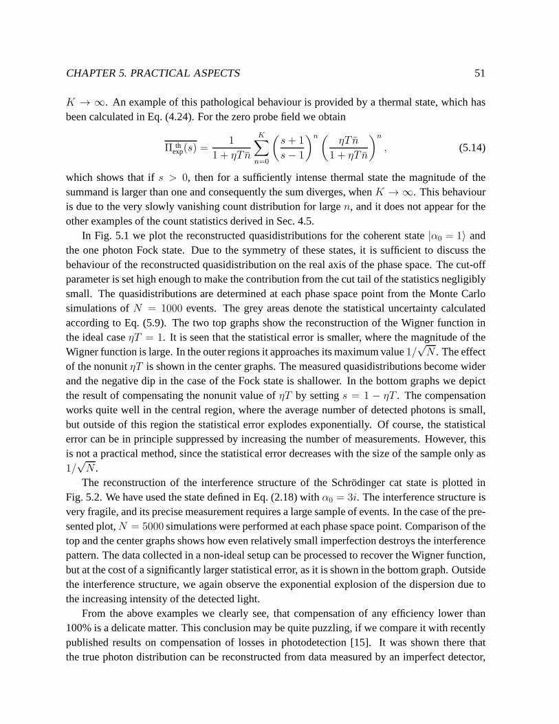
CHAPTER 5. PRACTICAL ASPECTS 51
K → ∞. An example of this pathological behaviour is provided by a thermal state, which hasbeen calculated in Eq. (4.24). For the zero probe field we obtain
Π thexp(s) =
1
1 + ηT n
K∑
n=0
(
s+ 1
s− 1
)n(ηT n
1 + ηT n
)n
, (5.14)
which shows that ifs > 0, then for a sufficiently intense thermal state the magnitudeof thesummand is larger than one and consequently the sum diverges, whenK → ∞. This behaviouris due to the very slowly vanishing count distribution for largen, and it does not appear for theother examples of the count statistics derived in Sec. 4.5.
In Fig. 5.1 we plot the reconstructed quasidistributions for the coherent state|α0 = 1〉 andthe one photon Fock state. Due to the symmetry of these states, it is sufficient to discuss thebehaviour of the reconstructed quasidistribution on the real axis of the phase space. The cut-offparameter is set high enough to make the contribution from the cut tail of the statistics negligiblysmall. The quasidistributions are determined at each phasespace point from the Monte Carlosimulations ofN = 1000 events. The grey areas denote the statistical uncertainty calculatedaccording to Eq. (5.9). The two top graphs show the reconstruction of the Wigner function inthe ideal caseηT = 1. It is seen that the statistical error is smaller, where the magnitude of theWigner function is large. In the outer regions it approachesits maximum value1/
√N . The effect
of the nonunitηT is shown in the center graphs. The measured quasidistributions become widerand the negative dip in the case of the Fock state is shallower. In the bottom graphs we depictthe result of compensating the nonunit value ofηT by settings = 1 − ηT . The compensationworks quite well in the central region, where the average number of detected photons is small,but outside of this region the statistical error explodes exponentially. Of course, the statisticalerror can be in principle suppressed by increasing the number of measurements. However, thisis not a practical method, since the statistical error decreases with the size of the sample only as1/√N .
The reconstruction of the interference structure of the Schrodinger cat state is plotted inFig. 5.2. We have used the state defined in Eq. (2.18) withα0 = 3i. The interference structure isvery fragile, and its precise measurement requires a large sample of events. In the case of the pre-sented plot,N = 5000 simulations were performed at each phase space point. Comparison of thetop and the center graphs shows how even relatively small imperfection destroys the interferencepattern. The data collected in a non-ideal setup can be processed to recover the Wigner function,but at the cost of a significantly larger statistical error, as it is shown in the bottom graph. Outsidethe interference structure, we again observe the exponential explosion of the dispersion due tothe increasing intensity of the detected light.
From the above examples we clearly see, that compensation ofany efficiency lower than100% is a delicate matter. This conclusion may be quite puzzling, if we compare it with recentlypublished results on compensation of losses in photodetection [15]. It was shown there thatthe true photon distribution can be reconstructed from datameasured by an imperfect detector,
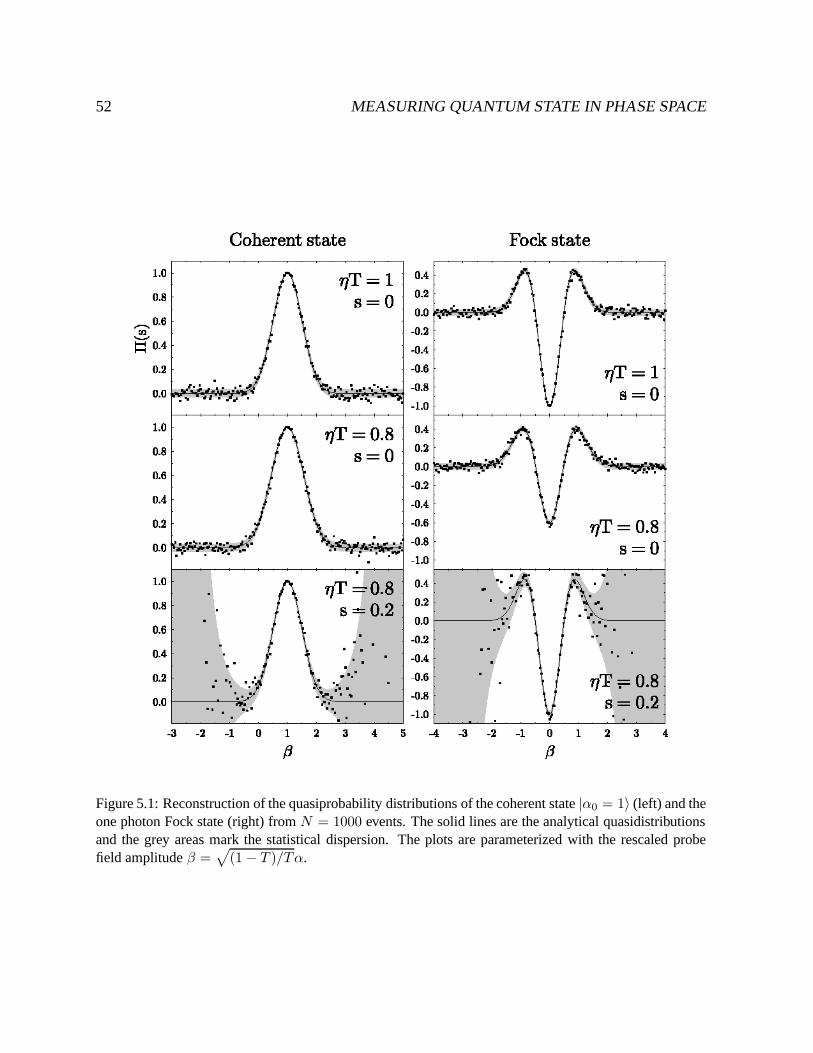
52 MEASURING QUANTUM STATE IN PHASE SPACE
Figure 5.1: Reconstruction of the quasiprobability distributions of the coherent state|α0 = 1〉 (left) and theone photon Fock state (right) fromN = 1000 events. The solid lines are the analytical quasidistributionsand the grey areas mark the statistical dispersion. The plots are parameterized with the rescaled probefield amplitudeβ =
√
(1− T )/Tα.

CHAPTER 5. PRACTICAL ASPECTS 53
Figure 5.2: Reconstruction of the interference structure of the Schrodinger cat state forα0 = 3i fromN = 5000 events at each point.
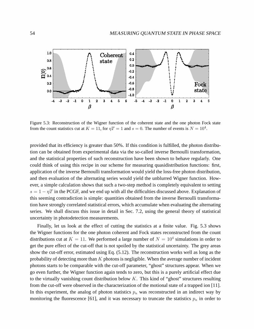
54 MEASURING QUANTUM STATE IN PHASE SPACE
Figure 5.3: Reconstruction of the Wigner function of the coherent state and the one photon Fock statefrom the count statistics cut atK = 11, for ηT = 1 ands = 0. The number of events isN = 104.
provided that its efficiency is greater than 50%. If this condition is fulfilled, the photon distribu-tion can be obtained from experimental data via the so-called inverse Bernoulli transformation,and the statistical properties of such reconstruction havebeen shown to behave regularly. Onecould think of using this recipe in our scheme for measuring quasidistribution functions: first,application of the inverse Bernoulli transformation wouldyield the loss-free photon distribution,and then evaluation of the alternating series would yield the unblurred Wigner function. How-ever, a simple calculation shows that such a two-step methodis completely equivalent to settings = 1− ηT in the PCGF, and we end up with all the difficulties discussed above. Explanation ofthis seeming contradiction is simple: quantities obtainedfrom the inverse Bernoulli transforma-tion have strongly correlated statistical errors, which accumulate when evaluating the alternatingseries. We shall discuss this issue in detail in Sec. 7.2, using the general theory of statisticaluncertainty in photodetection measurements.
Finally, let us look at the effect of cutting the statistics at a finite value. Fig. 5.3 showsthe Wigner functions for the one photon coherent and Fock states reconstructed from the countdistributions cut atK = 11. We performed a large number ofN = 104 simulations in order toget the pure effect of the cut-off that is not spoiled by the statistical uncertainty. The grey areasshow the cut-off error, estimated using Eq. (5.12). The reconstruction works well as long as theprobability of detecting more thanK photons is negligible. When the average number of incidentphotons starts to be comparable with the cut-off parameter,“ghost” structures appear. When wego even further, the Wigner function again tends to zero, butthis is a purely artificial effect dueto the virtually vanishing count distribution belowK. This kind of “ghost” structures resultingfrom the cut-off were observed in the characterization of the motional state of a trapped ion [11].In this experiment, the analog of photon statisticspn was reconstructed in an indirect way bymonitoring the fluorescence [61], and it was necessary to truncate the statisticspn in order to

CHAPTER 5. PRACTICAL ASPECTS 55
keep the error on a reasonably low level. We have seen that in the regions of the phase spacewhere a substantial part of the statisticspn is lost by the truncation, we do not have sufficientdata to determine the value of the Wigner function.
5.4 Mode mismatch
Another experimental imperfection that occurs in a realistic setup is the non-unit matching of themodes interfered at the high-transmission beam splitter BS. In order to analyse consequences ofthe mode mismatch, we will use the multimode approach developed in Sec. 4.4. Let us take thesignal field and the coherent probe field to be of the form
E(+)S (r, t) = aSuS(r, t) + V(r, t),
EP (r, t) = αuP (r, t) (5.15)
whereuS(r, t) anduP (r, t) are the corresponding normalized mode functions, and the operatorV(r, t) is the sum of all other signal modes remaining in the vacuum state. We will assume thatthe support of these mode functions lies within the domain defined by the detector surface andthe gate opening time. This allows us to write the normalization of the mode functions as
∫
∆t
dt∫
D
d2r |uS(r, t)|2 =
∫
∆t
dt∫
D
d2r |uP (r, t)|2 =
~ω0
2ǫ0c(5.16)
Further, we will assume that the overlap of the functionsuS(r, t) anduP (r, t) is real and positive.This can be always achieved by multiplyinguP (r, t) andα by appropriate conjugated phasefactors. We will denote
2ǫ0c
~ω0
∫
∆t
dt∫
D
d2r u
∗S(r, t)uP (r, t) =
√
ξ. (5.17)
Under these assumptions, we may represent the PCGF calculated from the count statisticsgiven by Eq. (4.14) in the form:
Π(s) =
⟨
: exp
(
− 2η
1− s[T a†S aS −
√
ξT (1− T )(a†Sα + aSα∗) + (1− T )|α|2]
)
:
⟩
(5.18)
Rearranging the terms in the exponent yields:
Π(s) =π(1− s)
2ηTWS
(√
ξ(1− T )
Tα;−1− s− ηT
ηT
)
exp
(
−2η(1− T )(1− ξ)
1− s|α|2
)
.
(5.19)Thus, if the signal and the probe modes are not matched perfectly, the PCGF is given by thequasidistribution function of the signal, but multiplied by a Gaussian envelopeexp[−2η(1 −
56 MEASURING QUANTUM STATE IN PHASE SPACE
T )(1− ξ)|α|2/(1− s)]. This envelope is centered at the origin of the phase space, and the fasterit decays, the larger is the mode mismatch, characterized bythe difference1 − ξ. Additionally,the parameterization of the signal quasidistribution is rescaled by
√ξ.
The effect of the mode-mismatch is more severe in outer regions of the phase space. It isnot important if the quasidistribution is localized aroundthe center of the phase space within thewidth of the Gaussian envelope. In particular, for the vacuum signal state we obtain:
Π(s) = exp
(
−2η(1− T )
1− s|α|2
)
. (5.20)
This result does not depend at all on the mode overlap parameterξ, simply because with the vac-uum signal field no interference occurs at the beam splitter BS and all the recorded photons comefrom the probe beam. The above expression can be interpretedas the quasidistribution functionof the signal mode characterized by the mode functionuP (r, t), which perfectly overlaps withthe probe field.
In a general case, we may rewrite Eq. (5.19) to the form:
Π(s) =π(1− s)
2ηTWS
(√
ξ(1− T )
Tα;−1− s− ηT
ηT
)
×π(1− s)
2ηTWvac
(√
(1− ξ)(1− T )
Tα;−1− s− ηT
ηT
)
, (5.21)
whereWvac(β; s) is the vacuum quasidistribution function. This representation allows us to in-terpret Eq. (5.19) as a two-mode quasidistribution which isa product of the signal mode qua-sidistribution and an additional vacuum quasidistribution. These two modes are probed at thephase space points proportional to
√ξα and
√1− ξα. The amplitude
√ξα describes the part
of the probe field that overlaps perfectly with the signal field, whereas√1− ξα corresponds to
the orthogonal remainder (orthogonality is understood here in the sense of the scalar productbetween the mode functions).
The parameterξ characterizing the overlap of the signal and the probe modescan be related tothe visibility of the interference. This expression will beuseful in the discussion of the practicalrealization of the scheme. Let as assume that the signal modeis in a coherent state|α0〉. Theintensity of the field measured by the photodetector is givenby
I = |√1− Tα−
√
ξTα0|2 + (1− ξ)T |α0|2, (5.22)
whereα is the amplitude of the coherent probe mode. It is seen that for givenα0 the minimumintensity is obtained for
√1− Tα =
√ξTα0, and it equals to:
Imin = (1− ξ)T |α0|2. (5.23)
CHAPTER 5. PRACTICAL ASPECTS 57
When we now vary with the phase ofα, keeping its absolute value fixed, the maximum intensityis achieved for
√1− Tα = −√
ξTα0, and its value is:
Imax = 4ξT |α0|2 + (1− ξ)T |α0|2. (5.24)
A simple calculation shows that the interference visibility v can be expressed using the overlapparameterξ as:
v =Imax− Imin
Imax+ Imin=
4ξ
2 + 2ξ. (5.25)
Inverting this relation, we obtain thatξ = v/(2− v).Finally, let us note that the effect of mode-mismatch in our scheme is quite different from
balanced homodyne detection, where it can be simply included in the overall detection efficiencyparameter. In our scheme, it generates a Gaussian envelope multiplying the measured quasidis-tribution function, and its importance depends on the probed point of the phase space.

58 MEASURING QUANTUM STATE IN PHASE SPACE

Chapter 6
Experiment
We shall now present direct measurement of the Wigner function by photon counting, using themethod presented in Chap. 4. Previous measurements of the Wigner function of light, performedat the University of Oregon [7] and Universitat Konstanz [10], were realizations of optical ho-modyne tomography. In our experiment, the Wigner function is determined directly from thestatistics of photocounts. Apart from the different principle of the measurement, we use a dif-ferent technique for light detection. As we discussed in Chap. 3, optical homodyne tomographyis based on detection of the signal light superposed on a strong, classical local oscillator. Thelight incident on photodetectors has macroscopic intensity, and it is converted into an electroniccurrent with the help ofp-i-n photodiodes. At this level of intensity, it is not possible to resolvecontributions from single photons, and the electric current is practically a continuous variable.Information on the quantum state of the measured light is contained in fluctuations of the differ-ence signal between two detectors. This signal is recorded using an analog-to-digital converter.
In our scheme, the intensity of the detected light is comparable with the intensity of the signalfield itself. Therefore, we need to use a detector that is sensitive to single optical photons. Cur-rently, the most efficient commercially available detectors on single-photon level are avalanchephotodiodes operated in the so-called Geiger mode. The Geiger mode of operation consists inbiasing the diode slightly above breakdown. Absorption of aphoton triggers the breakdown,which is a macroscopic, recordable event. The diode is placed in a circuit which quenches thebreakdown by lowering the voltage, and after a while restores the higher bias thus preparingthe diode for the detection of a next photon. The electronic signal obtained from the diode hasthe form of pulses of uniform height and duration, which correspond to single detection events.These pulses, after shaping, can be counted using a standarddigital logic device.
We open this chapter with a review of the principle of the measurement in Sec. 6.1. Theexperimental setup is described in Sec. 6.2, and the resultsof the measurements are reported inSec. 6.3. In Sec. 6.4 we discuss the effect of various experimental factors, and summarize thepresentation of the experiment.
59

60 MEASURING QUANTUM STATE IN PHASE SPACE
6.1 Principle
In order to make the presentation of the experiment self-contained, let us start with a brief reviewof the principle of the measurement. The Wigner function at agiven phase space point is itself awell defined quantum observable. Furthermore, the measurement of this observable can be im-plemented for optical fields using an arrangement employingan auxiliary coherent probe beam.The amplitude and the phase of the probe field define the point in the phase space at which theWigner function is measured. This allows one to scan the phase space point-by-point, simply bychanging the parameters of the probe field.
Our experiment is based on the representation of the Wigner function at a complex phasespace point denoted byα as the expectation value of the following operator:
W (α) =2
π
∞∑
n=0
(−1)nD(α)|n〉〈n|D†(α), (6.1)
whereD(α) is the displacement operator and|n〉 denote Fock states,n|n〉 = n|n〉. Thus,W (α)
has two eigenvalues:2/π and−2/π, corresponding to degenerate subspaces spanned respec-tively by even and odd displaced Fock states. Practical means to translate this formula into anoptical arrangement are quite simple. The displacement transformation can be realized by super-posing the measured field at a low-reflection beam splitter with a strong coherent probe beam.The value of the displacementα is equal in this setup to the reflected amplitude of the probefield. Furthermore, the projections on Fock states can be obtained by photon counting assumingunit quantum efficiency. These two procedures, combined together, provide a practical way tomeasure the Wigner function at an arbitrarily selected phase space pointα.
6.2 Setup
The experimental setup we used to measure the Wigner function is shown schematically inFig. 6.1. In principle, it is a Mach-Zender interferometricscheme with the beams in two armsof the interferometer serving as the signal and the probe fields. An attenuated, linearly polarized(in the plane of Fig. 4.1) 632.8 nm beam from a frequency-stabilized single-mode He:Ne laseris divided by a low-reflection beam splitter BS1. The weak reflected beam is used to generatethe signal field whose Wigner function will be measured. The state preparation stage consistsof a neutral density filter ND and a mirror mounted on a piezoelectric translator PZT. With thisarrangement, we are able to create pure coherent states withvariable phase as well as their in-coherent mixtures. Though these states do not exhibit nonclassical properties, they constitute anontrivial family to demonstrate the principle of the method, which provides complete charac-terization of both quantum and classical field fluctuations.
The strong beam leaving the beam splitter BS1 plays the role of the probe field with whichwe perform the displacement transformationD(α). In order to scan the phase space one should
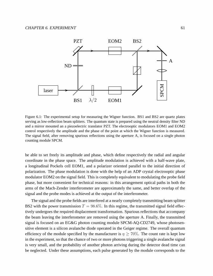
CHAPTER 6. EXPERIMENT 61
ND
laser
BS1 λ/2 EOM1
PZT EOM2 BS2
A
SP
CM
Figure 6.1: The experimental setup for measuring the Wignerfunction. BS1 and BS2 are quartz platesserving as low-reflection beam splitters. The quantum stateis prepared using the neutral density filter NDand a mirror mounted an a piezoelectric translator PZT. The electrooptic modulators EOM1 and EOM2control respectively the amplitude and the phase of the point at which the Wigner function is measured.The signal field, after removing spurious reflections using the aperture A, is focused on a single photoncounting module SPCM.
be able to set freely its amplitude and phase, which define respectively the radial and angularcoordinate in the phase space. The amplitude modulation is achieved with a half-wave plate,a longitudinal Pockels cell EOM1, and a polarizer oriented parallel to the initial direction ofpolarization. The phase modulation is done with the help of an ADP crystal electrooptic phasemodulator EOM2 on the signal field. This is completely equivalent to modulating the probe fieldphase, but more convenient for technical reasons: in this arrangement optical paths in both thearms of the Mach-Zender interferometer are approximately the same, and better overlap of thesignal and the probe modes is achieved at the output of the interferometer.
The signal and the probe fields are interfered at a nearly completely transmitting beam splitterBS2 with the power transmissionT = 98.6%. In this regime, the transmitted signal field effec-tively undergoes the required displacement transformation. Spurious reflections that accompanythe beam leaving the interferometer are removed using the aperture A. Finally, the transmittedsignal is focused on an EG&G photon counting module SPCM-AQ-CD2749, whose photosen-sitive element is a silicon avalanche diode operated in the Geiger regime. The overall quantumefficiency of the module specified by the manufacturer isη ≥ 70%. The count rate is kept lowin the experiment, so that the chance of two or more photons triggering a single avalanche signalis very small, and the probability of another photon arriving during the detector dead time canbe neglected. Under these assumptions, each pulse generated by the module corresponds to the

62 MEASURING QUANTUM STATE IN PHASE SPACE
detection of a single photon1. The pulses are acquired by a computer, which also controls thevoltages applied to the electrooptic modulators. The interference visibility in our setup has beenmeasured to bev ≥ 98.5%, and the phase difference between the two arms was stable up to fewpercent over times of the order of ten minutes.
6.3 Results
The voltages applied to electrooptic modulators were generated by high-voltage power suppliescontrolled by analog output ports of a multifunction I/O card (National Instruments PCI-MIO-16E-4). A typical scan of the phase space consisted of sampling a sequence of circles withincreasing radius. This was because changing the voltage applied to the amplitude modulatorrequired a settling time of the order of 1 s. For a fixed amplitude the phase could be scannedmuch faster, as the phase modulator driver had the bandwidthup to 10 kHz. For a selected pointof the phase space, the photon statistics was collected using a digital counter on the same I/Ocard, operated in the buffered event counting mode.
In Fig. 6.2 we depict the measured Wigner functions of the vacuum, a weak coherent state,and a phase diffused coherent state. Phase fluctuations wereobtained by applying a 400 Hz sinewaveform to the piezoelectric translator. For all the plots, the phase space was scanned on a griddefined by 20 amplitudes and 40 phases. The scaling of the radial coordinate is obtained fromthe average number of photonsnvac detected for the blocked signal path. Thus the graphs areparameterized with the complex variableβ = eiϕn
1/2vac , whereϕ is the phase shift generated by
the phase modulator EOM2. At each selected point of the phasespace, the photocount statisticspn(β) was determined from a sequence ofN = 8000 counting intervals, eachτ = 30µs long.The duration of the counting intervalτ defines the temporal envelope of the measured mode. Thecount statistics was used to evaluate the alternating sum2
Π(β) =
∞∑
n=0
(−1)npn(β), (6.2)
which, up to the normalization factor2/π is equal to the Wigner function of the measured state.Statistical variance of this result can be estimated by Var[Π(β)] = {1 − [Π(β)]2}/N , accordingto the discussion in Sec. 5.2. Thus, the statistical error ofour measurement reaches its maximumvalue, equal to1/N1/2 ≈ 1.1%, when the value of the Wigner function is close to zero.
1The operating mode of the SPCM results in a certain amount of extraneous pulses originating from dark countsand afterpulsing. The dark count rate of our module is less than 100 s−1. This gives on average< 3 · 10−3 during asingle counting interval, which is 30µs long. The typical afterpulsing probability is0.2%. Thus, both these effectsgive a negligible contribution to the measured count statistics.
2Here we explicitly write dependence ofΠ on the phase space pointβ. The numbers used in the previouschapter as a parameter ofΠ is now fixed and equal to zero. The operational phase space point β can be expressedby the amplitudeα of the probe field asβ =
√
η(1 − T )α.
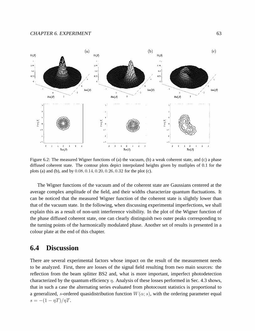
CHAPTER 6. EXPERIMENT 63
Figure 6.2: The measured Wigner functions of (a) the vacuum,(b) a weak coherent state, and (c) a phasediffused coherent state. The contour plots depict interpolated heights given by mutliples of 0.1 for theplots (a) and (b), and by0.08, 0.14, 0.20, 0.26, 0.32 for the plot (c).
The Wigner functions of the vacuum and of the coherent state are Gaussians centered at theaverage complex amplitude of the field, and their widths characterize quantum fluctuations. Itcan be noticed that the measured Wigner function of the coherent state is slightly lower thanthat of the vacuum state. In the following, when discussing experimental imperfections, we shallexplain this as a result of non-unit interference visibility. In the plot of the Wigner function ofthe phase diffused coherent state, one can clearly distinguish two outer peaks corresponding tothe turning points of the harmonically modulated phase. Another set of results is presented in acolour plate at the end of this chapter.
6.4 Discussion
There are several experimental factors whose impact on the result of the measurement needsto be analyzed. First, there are losses of the signal field resulting from two main sources: thereflection from the beam splitter BS2 and, what is more important, imperfect photodetectioncharacterized by the quantum efficiencyη. Analysis of these losses performed in Sec. 4.3 shows,that in such a case the alternating series evaluated from photocount statistics is proportional toa generalized,s-ordered quasidistribution functionW (α; s), with the ordering parameter equals = −(1 − ηT )/ηT .

64 MEASURING QUANTUM STATE IN PHASE SPACE
In addition, the two modes interfered at the beam splitter BS2 are never matched perfectly.The effects of the mode mismatch have been analysed in Sec. 5.4. We will now apply thisanalysis to the experimental results, but first let us recallbriefly the physical picture of modemismatch. For this purpose, we need to consider the normalized mode functions describing thetransmitted signal field and the reflected probe field. The squared overlapξ of these two modefunctions can be related to the interference visibilityv asξ = v/(2− v). In order to describe theeffects of the mode mismatch, we need to decompose the probe mode function into a part thatprecisely overlaps with the signal, and the orthogonal remainder. The amplitude of the probefield effectively interfering with the signal is thus multiplied by ξ1/2, and the remaining part ofthe probe field contributes to independent Poissonian counts with the average number of detectedphotons equal(1− ξ)|β|2. Consequently, the full count statistics is given by a convolution of thestatistics generated by the interfering fields, and the Poissonian statistics of mismatched photons.A simple calculation shows, that the alternating sum evaluated from such a convolution can berepresented as a product of the contributions corresponding to the two components of the probefield:
Π(β) = exp[−2(1− ξ)|β|2]
× π
2ηTW
(√
ξ
ηTβ;−1− ηT
ηT
)
. (6.3)
Here on the right-hand side we have made use of the theoretical results for imperfect detectionobtained in Secs. 4.3 and 5.4. Specializing the above resultto a coherent signal state|α0〉 withthe amplitudeα0, yields:
Π(β) = exp[−2|β −√
ξηTα0|2 − 2(1− ξ)ηT |α0|2]. (6.4)
Thus, in a realistic caseΠ(β) represents a Gaussian centered at the attenuated amplitude√ξηTα0,
and the width remains unchanged. This Gaussian function in multiplied by the constant factorexp[−2(1 − ξ)ηT |α0|2]. For our measurement,ξ ≈ 97% andηT |α0|2 ≈ 1.34, which gives thevalue of this factor equal 0.92. This result agrees with the height of the experimentally measuredWigner function of a coherent state.
In Fig. 6.3 we compare the phase-averaged measured Wigner function for the vacuum statewith theoretical predictions. Agreement between the experimental points and the Gaussian curveis very good. This plot can be used to estimate the amount of excess thermal noise in the laserradiation. Let us assume that from the averagenvac = |β|2 registered photons a constant fractionκth originates from thermal noise. TheP -representation of the field that is effectively detected isgiven by
P (γ) =1
πκth|β|2exp
(
−|γ −√1− κthβ|2
κth|β|2)
. (6.5)
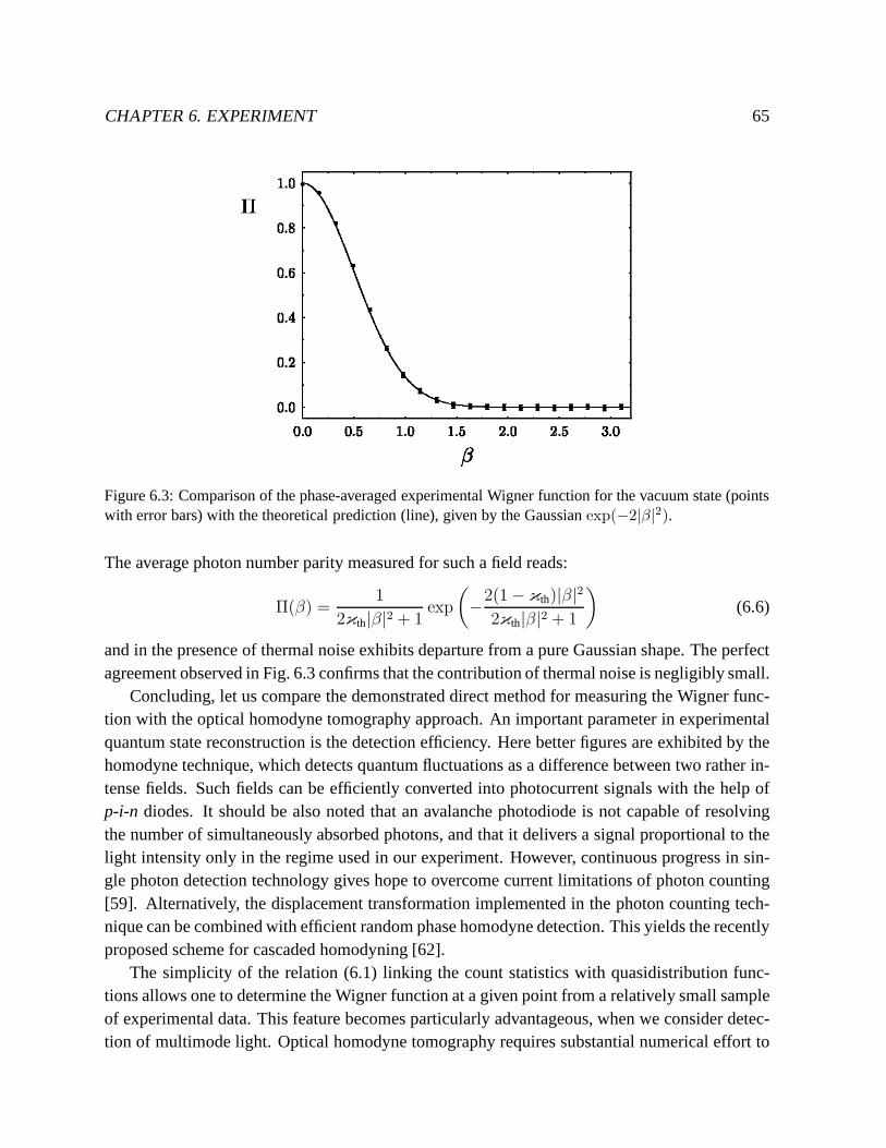
CHAPTER 6. EXPERIMENT 65
Figure 6.3: Comparison of the phase-averaged experimentalWigner function for the vacuum state (pointswith error bars) with the theoretical prediction (line), given by the Gaussianexp(−2|β|2).
The average photon number parity measured for such a field reads:
Π(β) =1
2κth|β|2 + 1exp
(
−2(1− κth)|β|22κth|β|2 + 1
)
(6.6)
and in the presence of thermal noise exhibits departure froma pure Gaussian shape. The perfectagreement observed in Fig. 6.3 confirms that the contribution of thermal noise is negligibly small.
Concluding, let us compare the demonstrated direct method for measuring the Wigner func-tion with the optical homodyne tomography approach. An important parameter in experimentalquantum state reconstruction is the detection efficiency. Here better figures are exhibited by thehomodyne technique, which detects quantum fluctuations as adifference between two rather in-tense fields. Such fields can be efficiently converted into photocurrent signals with the help ofp-i-n diodes. It should be also noted that an avalanche photodiodeis not capable of resolvingthe number of simultaneously absorbed photons, and that it delivers a signal proportional to thelight intensity only in the regime used in our experiment. However, continuous progress in sin-gle photon detection technology gives hope to overcome current limitations of photon counting[59]. Alternatively, the displacement transformation implemented in the photon counting tech-nique can be combined with efficient random phase homodyne detection. This yields the recentlyproposed scheme for cascaded homodyning [62].
The simplicity of the relation (6.1) linking the count statistics with quasidistribution func-tions allows one to determine the Wigner function at a given point from a relatively small sampleof experimental data. This feature becomes particularly advantageous, when we consider detec-tion of multimode light. Optical homodyne tomography requires substantial numerical effort to

66 MEASURING QUANTUM STATE IN PHASE SPACE
reconstruct the multimode Wigner function. In contrast, the photon counting method has a veryelegant generalization to the multimode case: after applying the displacement to each of the in-volved modes, the Wigner function at the selected point is simply given by the average parity ofthe total number of detected photons. Moreover, the dichotomic outcome of such a measurementprovides a novel way of testing quantum nonlocality exhibited by correlated states of opticalradiation [63].
Chapter 7
Statistical uncertainty in photodetectionmeasurements
In this chapter, we shall study the problem of statistical uncertainty from a more general point ofview. Over recent years, the set of tools for measuring quantum statistical properties of opticalradiation has substantially enlarged. In addition to the techniques discussed in this thesis: dou-ble homodyne detection, optical homodyne tomography, and the direct method for measuringquasidistribution functions, other novel schemes have been proposed [64, 65, 66, 67, 68]. Thequantum optical “toolbox” for measuring light contains nowexperimentally established schemesfor reconstructing various representations of its quantumstate: theQ function, the Wigner func-tion, and the density matrix in the quadrature and the Fock bases. A device that is used in mostof quantum optical schemes to convert the quantum signal to amacroscopic level is the photode-tector. Thus, photodetection is a basic ingredient of quantum optical measurements.
The quantum state can be characterized using various representations: quasidistribution func-tions or a density matrix in a specific basis. From a theoretical point of view, all these forms areequivalent. Each representation contains complete information on the quantum state, and theycan be transformed from one to another. Any observable related to the measured systems can beevaluated from an arbitrary representation using an appropriate expression [69].
This simple picture becomes much more complicated when we deal with real experimentaldata rather than analytical formulae. Each quantity determined from a finite number of exper-imental runs is affected by a statistical error. Consequently, the density matrix or the quasidis-tribution function reconstructed from the experimental data is known only with some statisticaluncertainty. This uncertainty is important when we furtheruse the reconstructed information tocalculate other observables or to pass to another representation. The crucial question is, whetherdetermination of a certain representation with sufficient accuracy guarantees that arbitrary ob-servable can be calculated from these data with a reasonablylow statistical error. If this is notthe case, the reconstructed information on the quantum state of the measured system turns outto be somewhat incomplete. Furthermore, transformation between various representations of the
67

68 MEASURING QUANTUM STATE IN PHASE SPACE
quantum state becomes a delicate matter.
These and related problems call for a rigorous statistical analysis of quantum optical mea-surements. We shall provide here complete statistical description of a measurement of quantumobservables in optical schemes based on photodetection. This approach fully characterizes sta-tistical properties of quantities determined in a realistic measurement from a finite number ofexperimental runs. It can be applied either to determination of a single quantum observable,or to the reconstruction of the quantum state in a specific representation. Within the presentedframework we study, using a simple example, the completeness of the experimentally recon-structed information on the quantum state. We demonstrate the pathological behavior suggestedabove, when the reconstructed data cannot be used to calculate certain observables due to rapidlyexploding statistical errors. Our example is motivated by the direct scheme for measuring qua-sidistribution functions of light.
Compared to previous works on statistical noise, our attention will be focused here on two im-portant statistical aspects of quantum state measurement.First, we shall go beyond the minimumsecond-order treatment of the statistical error [50, 51, 52] and provide, in a closed mathematicalform, a complete statistical description of quantum observables determined from realistic mea-surements. This result, derived from the first principles without using any approximations, isan exact analytical solution to the problem which so far has been approached only by means ofMonte Carlo simulations [46, 49]. The second problem discussed here will be the feasibility ofreconstructing the quantum state from realistic, finite data collected in a specific experimentalscheme. It is generally believed that a sufficient conditionfor successful reconstruction is theexistence of the covariance matrix with finite elements [15,16, 17]. We point out that this beliefmisses an important issue resulting from statistical uncertainty. Suppose we have reconstructeda family of observables with finite statistical variances. In order to be sure that the reconstructedinformation on the quantum state is accurate and complete, we should ask the following question:can we always use these observables to evaluate any quantum property of the measured systemthat can be expressed in terms of the reconstructed family? We shall give a clear negative answerto this question, based on a detailed discussion of carefully selected counterexamples. Althoughall observables involved in these examples are representedby bounded, well-defined operators,statistical fluctuations are shown to be arbitrarily huge, when the reconstructed family is furtherused to evaluate certain quantum expectation values. This singular behaviour is quantitatively ex-plained as a result of strong statistical correlations between observables reconstructed from thesame sample of experimental data. Consequently, the discussed examples clearly demonstratethat statistical properties of reconstructed observablesdepend in an essential way on a specificexperimental scheme, which effectively limits available information on the measured system.
This chapter is organized as follows. The starting point of our analysis is the probabilitydistribution of obtaining a specific histogram fromN runs of the experimental setup. This basicquantity determines all statistical properties of quantumobservables reconstructed from a finitesample of experimental data. We characterize these properties using the generating function,

CHAPTER 7. STATISTICAL UNCERTAINTY. . . 69
for which we derive an exact expression directly from the probability distribution of the exper-imental outcomes. These general results are presented in Sec. 7.1. Then, in Sec. 7.2, we usethe developed formalism to discuss the reconstruction of the photon number distribution of asingle light mode, and its subsequent utilization to evaluate the parity operatorΠ. We considertwo experimental schemes: direct photon counting using an imperfect detector, and homodynedetection with random phase. In both the cases we find that theevaluation of the parity operatorfrom the reconstructed photon statistics is a very delicatematter. For photon counting of a ther-mal state, we show that neither the statistical mean value ofΠ nor its variance have to exist whenwe take into account arbitrarily high count numbers. For random phase homodyne detection, thestatistical error of the parity operator is an interplay of the number of runsN and the specificregularization method used for its evaluation. The exampleof the parity operator illustrates diffi-culties related to the transformations between various experimentally determined representationsof the quantum state, as the parity operator yields, up to a multiplicative constant, the Wignerfunction at the phase space origin. Finally, in Sec. 7.3 we discuss consequences of statisticaluncertainty in the measurements of the quantum state.
7.1 Statistical analysis of experiment
In photodetection measurements, the raw quantity delivered by a single experimental run is thenumber of photoelectrons ejected from the active material of the detectors. The data recordedfor further processing depends on a specific scheme. It may bejust the number of counts ona single detector, or a difference of photocounts on a pair ofphotodetectors, which is the caseof balanced homodyne detection. It may also be a finite sequence of integer numbers, e.g. fordouble homodyne detection. We will denote in general this data byn, keeping in mind all thepossibilities.
The experimental scheme may have some external parametersθ, for example the phase ofthe local oscillator in homodyne detection. The series of measurements are repeated for varioussettingsθi of these parameters. Thus, what is eventually obtained fromthe experiment, is aset of histograms{kn}θi, telling in how many runs with the settingsθi the outcomen has beenrecorded. We assume that for each setting the same total number ofN runs has been performed.
The theoretical probabilitypn(θi) of obtaining the outcomen in a run with settingsθi isgiven by the expectation value of a positive operator-valued measure (POVM)pn(θi) acting inthe Hilbert space of the measured system. The reconstruction of an observableA is possible, if itcan be represented as a linear combination of the POVMs for the settings used in the experiment:
A =∑
i
∑
n
an(θi)pn(θi), (7.1)
wherean(θi) are the kernel functions. The above formula allows one to compute the quantumexpectation value〈A〉 from the probability distributionspn(θi) = 〈pn(θi)〉.
70 MEASURING QUANTUM STATE IN PHASE SPACE
This theoretical relation has to be applied now to the experimental data. The simplest andthe most commonly used strategy is to estimate the probability distributionspn(θi) by experi-mental relative frequencies(kn/N)θi. The relative frequencies integrated with the appropriatekernel functions yield an estimate for the expectation value of the operatorA. For simplicity, wewill denote this estimate just byA. Thus, the recipe for reconstructing the observableA fromexperimental data is given by the counterpart of Eq. (7.1):
A =∑
i
∑
n
an(θi)
(
knN
)
θi
. (7.2)
We will now analyse statistical properties of the observableA evaluated according to Eq. (7.2)from data collected in a finite number of experimental runs. Our goal is to characterize thestatistical distributionw(A) defining the probability that the experiment yields a specific resultA. The fundamental object in this analysis is the probabilityP({kn}; θ) of obtaining a specifichistogram{kn} for the settingsθ. In order to avoid convergence problems, we will restrict thepossible values ofn to a finite set by introducing a cut-off. The probabilityP({kn}; θ) is thengiven by the multinomial distribution [60]:
P({kn}; θ) =N !
(N −∑′n kn)!
(
1−∑
n
′pn(θ)
)N−∑′
nkn∏
n
′ 1
kn![pn(θ)]
kn, (7.3)
where prim in sums and products denotes the cut-off. This distribution describing experimentalhistograms is derived from an assumption that all the detection events are statistically indepen-dent.
Let us first consider a contributionAi to the observableA calculated from the histogramθi:
Ai =∑
n
′an(θi)
(
knN
)
θi
. (7.4)
Its statistical distributionw(Ai; θi) is given by the following sum over all possible histogramsthat can be obtained fromN experimental runs:
w(Ai; θi) =∑
{kn}
P({kn}; θi)δ(
Ai −1
N
∑
n
′an(θi)kn
)
. (7.5)
Equivalently, the statistics ofAi can be characterized by the generating functionw(λ; θi) for themoments, which is the Fourier transform of the distributionw(Ai; θi):
w(λ; θi) =
∫
dAi eiλAiw(Ai; θi)
=∑
{kn}
P({kn}; θi) exp(
iλ
N
∑
n
′an(θi)kn
)
. (7.6)

CHAPTER 7. STATISTICAL UNCERTAINTY. . . 71
An easy calculation yields the explicit form of the generating function:
w(λ; θi) =
(
1 +∑
n
′pn(θi)(e
iλan(θi)/N − 1)
)N
. (7.7)
The observableA is obtained via summation of the componentsAi corresponding to all settingsof the external parametersθi. As these components are determined from disjoint subsets of theexperimental data, they are statistically independent. Consequently, the generating functionw(λ)for the moments of the observableA is given by the product:
w(λ) =
∫
dA eiλAw(A) =∏
i
w(λ; θi)
=∏
i
(
1 +∑
n
′pn(θi)(e
iλan(θi)/N − 1)
)N
. (7.8)
This expression contains the complete statistical information on determination of the observableA from a finite number of runs of a specific experimental setup. The measuring apparatus isincluded in this expression in the form of a family of POVMspn(θi). The quantum expectationvalue of these POVMs over the state of the measured system yields the probability distributionspn(θi). Finally, the coefficientsan(θi) are given by the computational recipe for reconstructingthe observableA from the measured distributions. The analytical expression for the generatingfunction given in Eq. (7.8), derived from the exact description of raw experimental outcomes,provides a complete characterization of statistical fluctuations in realistic measurements of quan-tum observables. Let us note that in general the generating functionw(λ) cannot be expressed bythe operatorA alone. Both the POVMspn(θi) and the kernel functionsan(θi) enter Eq. (7.8) ina nontrivial way, which clearly shows that statistical properties of the reconstructed observabledepend essentially on the specific measurement scheme.
The basic characteristics of statistical properties of theobservableA is provided by the meanvalue E(A) and the variance Var(A). These two quantities can be easily found by differentiatingthe logarithm of the generating operator:
E(A) :=1
i
ddλ
log w(λ)
∣
∣
∣
∣
λ=0
=∑
i
∑
n
′an(θi)pn(θi), (7.9)
Var(A) :=1
i2d2
dλ2log w(λ)
∣
∣
∣
∣
λ=0
=1
N
∑
i
∑
n
′a2n(θi)pn(θi)−
∑
i
(
∑
n
′an(θi)pn(θi)
)2
. (7.10)
The statistical error is scaled with the inverse of the square root of the number of runsN . Let usnote that the second component in the derived formula for Var(A) differs from that used in the
72 MEASURING QUANTUM STATE IN PHASE SPACE
discussions of homodyne tomography in Refs. [50, 52], whereit was equal just to[E(A)]2. Thisdifference results from different assumptions about the local oscillator phase: in Refs. [50, 52]it was considered to be a uniformly distributed stochastic variable in order to avoid systematicerrors, whereas we have assumed that the number of runs is fixed for each selected setting of theexternal parameters.
The goal of quantum state measurements is to retrieve the maximum amount of informa-tion on the quantum state available from the experimental data. Therefore the experimentalhistograms are usually processed many times in order to reconstruct a family of observablescharacterizing the quantum state. Of course, quantities determined from the same set of exper-imental data are not statistically independent, but in general exhibit correlations. The analysispresented above can be easily extended to the evaluation of any number of observables from thesame sample of experimental data. If we restrict our attention to the basic, second-order char-acterization of these correlations, it is sufficient to discuss simultaneous determination of twoobservables. Let us suppose that in addition toA, another observableB has been calculatedfrom the histograms{kn}θi according to the formula:
B =∑
i
∑
n
′bn(θi)
(
knN
)
θi
. (7.11)
The generating functionw(λ, µ) corresponding to the joint probability distributionw(A,B) canbe found analogously to the calculations presented above. The final result is:
w(λ, µ) =
∫
dAdB eiλA+iµBw(A,B)
=∏
i
(
1 +∑
n
′pn(θi)(e
iλan(θi)/N+iµbn(θi)/N − 1)
)N
. (7.12)
The covariance between the experimentally determined values ofA andB is given by:
Cov(A,B) :=1
i2d2
dλdµlog w(λ, µ)
∣
∣
∣
∣
λ,µ=0
=1
N
∑
i
[
∑
n
′an(θi)bn(θi)pn(θi)−
(
∑
n
′an(θi)pn(θi)
)(
∑
m
′bm(θi)pm(θi)
)]
.
(7.13)
The covariance can be normalized to the interval[−1, 1] using Var(A) and Var(B), which yieldsthe correlation coefficient for the pair of observablesA andB:
Corr(A,B) :=Cov(A,B)
√
Var(A)Var(B). (7.14)

CHAPTER 7. STATISTICAL UNCERTAINTY. . . 73
This quantity defines whether the statistical deviations ofA andB tend to have the same oropposite sign, which corresponds respectively to the positive or negative value of Corr(A,B).
We have assumed that the histogramskn have been measured for a finite number of externalparameters settingsθi, which is always the case in an experiment. However, in some schemes themeasurement of histograms is in principle necessary for allvalues of a continuous parameter. Forexample, in optical homodyne tomography the full information on the quantum state is containedin a family of quadrature distributions for all local oscillator phases. Restriction to a finite set ofphases introduces a systematic error to the measurement [50, 70].
7.2 Phase-insensitive detection of a light mode
We will now apply the general formalism developed in the preceding section to the reconstruc-tion of phase-independent properties of a single light mode. The basic advantage of this exem-plary system is that it will allow us to discuss, in a very transparent way, pathologies resultingfrom the statistical uncertainty. All phase-independent properties of a single light mode arefully characterized by its photon number distributionρν . Therefore, it is sufficient to apply aphase-insensitive technique to measure the photon statistics of the field. We will consider twomeasurement schemes that can be used for this purpose: direct photon counting and randomphase homodyne detection.
The photon number distribution is given by the expectation value of a family of projectionoperatorsρν = |ν〉〈ν|, where|ν〉 is theνth Fock state. In principle, knowledge of this distributionenables us to evaluate any phase-independent observable related to the measured field. A simpleyet nontrivial observable, which we will use to point out difficulties with the completeness of thereconstructed information on the quantum state, is the parity operator:
Π =
∞∑
ν=0
(−1)ν |ν〉〈ν|. (7.15)
This operator is bounded, and well defined on the complete Hilbert space of a single light mode.Its expectation value is given by the alternating series of the photon number distribution:
〈Π〉 =∞∑
ν=0
(−1)ν〈ρν〉, (7.16)
which is absolutely convergent for any quantum state. Therefore, any pathologies connected toits determination from experimental data, if there appear any, cannot be ascribed to its singularanalytical properties.

74 MEASURING QUANTUM STATE IN PHASE SPACE
7.2.1 Direct photon counting
First, we will consider the reconstruction of phase insensitive properties of a single light modefrom data measured using a realistic, imperfect photodetector. The positive operator-valued mea-surepn describing the probability of ejectingn photoelectrons from the detector is given by [71]:
pn = :(ηa†a)n
n!exp(−ηa†a) :, (7.17)
wherea is the annihilation operator of the light mode, andη is the quantum efficiency of thephotodetector. In the limitη → 1 we get directlypn = |n〉〈n|. In a general case, the probabilitydistribution for the photoelectron number is related to thephoton statistics via the Bernoullitransformation. This relation can be analytically inverted [15], which yields the expression:
ρν =
∞∑
n=0
r(η)νn pn, (7.18)
where the kernel functionsr(η)νn are given by:
r(η)νn =
0, n < ν,
1
ην
(
n
ν
)(
1− 1
η
)n−ν
, n ≥ ν.(7.19)
The inversion formula has a remarkable property thatρν depends only on the “tail” of the pho-tocount statistics forn ≥ ν. It has been shown that the inverse transformation can be applied toexperimentally determined photocount statistics for an arbitrary state of the field, provided thatthe detection efficiency is higher that 50% [15].
We will now discuss statistical properties of the photon number distribution determined byphoton counting within the general framework developed in Sec. 7.1. The case of perfect de-tection is trivial for statistical analysis. Therefore we will consider nonunit detection efficiency,which is numerically compensated in the reconstruction process using the inverse Bernoulli trans-formation according to Eq. (7.18). For all examples presented here, the efficiency isη = 80%,which is well above the50% stability limit.
In Fig. 7.1 we depict the reconstructed photon number distributions for a coherent state, athermal state, and a squeezed vacuum state. The mean values E(ρν) along with their statisticalerrors[Var(ρν)]1/2 are compared with Monte Carlo realizations of a photon counting experiment,with the number of runsN = 4000. It is seen that for a thermal state and a squeezed vacuumstate, the statistical error of the probabilitiesρν grows unlimitedly with the photon numberν.However, any experimental histogram obtained from a finite number of runs ends up for a cer-tain count number, and therefore the reconstructed photon statistics is zero above this number.An important feature that is evidently seen in the Monte Carlo simulations, are correlations be-tween the consecutive matrix elements. The reconstructed photon number distribution clearly
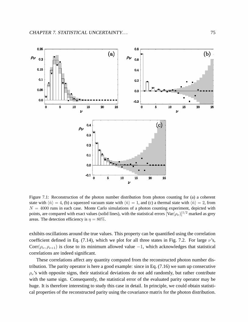
CHAPTER 7. STATISTICAL UNCERTAINTY. . . 75
Figure 7.1: Reconstruction of the photon number distribution from photon counting for (a) a coherentstate with〈n〉 = 4, (b) a squeezed vacuum state with〈n〉 = 1, and (c) a thermal state with〈n〉 = 2, fromN = 4000 runs in each case. Monte Carlo simulations of a photon counting experiment, depicted withpoints, are compared with exact values (solid lines), with the statistical errors[Var(ρν)]1/2 marked as greyareas. The detection efficiency isη = 80%.
exhibits oscillations around the true values. This property can be quantified using the correlationcoefficient defined in Eq. (7.14), which we plot for all three states in Fig. 7.2. For largeν’s,Corr(ρν , ρν+1) is close to its minimum allowed value−1, which acknowledges that statisticalcorrelations are indeed significant.
These correlations affect any quantity computed from the reconstructed photon number dis-tribution. The parity operator is here a good example: sincein Eq. (7.16) we sum up consecutiveρν ’s with opposite signs, their statistical deviations do notadd randomly, but rather contributewith the same sign. Consequently, the statistical error of the evaluated parity operator may behuge. It is therefore interesting to study this case in detail. In principle, we could obtain statisti-cal properties of the reconstructed parity using the covariance matrix for the photon distribution.

76 MEASURING QUANTUM STATE IN PHASE SPACE
Figure 7.2: The correlation coefficient between the consecutive density matrix elements Corr(ρν , ρν+1),depicted for the coherent state (◦), the squeezed state (�), and the thermal state (∗) from Fig. 7.1.
However, it will be more instructive to express the parity directly in terms of the photocountstatistics, and then to apply the statistical analysis to this reconstruction recipe. This route iscompletely equivalent to studying evaluation of the parityvia the photon number distribution, asall transformations of the experimental data, which we consider here, are linear.
A simple calculation combining Eqs. (7.15) and (7.18) showsthat:
Π =
K∑
n=0
(
1− 2
η
)n
pn, (7.20)
where we have introduced in the upper summation limit a cut-off parameterK for the photocountnumber. This formula clearly demonstrates pathologies related to the determination of the parityoperator. For anyη < 1, the factor(1 − 2/η)n is not bounded, which makes the convergence ofthe whole series questionable in the limitK → ∞. Of course, for an experimental histogram thesummation is always finite, but the exploding factor amplifies contribution from the “tail” of thehistogram, where usually only few events are recorded, and consequently statistical errors aresignificant.
Let us study these pathologies more closely using examples of a coherent state and a thermalstate. For a coherent state|α〉, both the expressions for E(Π) and Var(Π) are convergent withK → ∞. However, the variance, given by the formula:
Var(Πcoh) =1
N
[
exp
(
4(1− η)
η|α|2)
− exp(−4|α|2)]
, (7.21)
grows very rapidly with the coherent state amplitudeα, when the number of runsN is fixed.For a thermal state with the average photon numbern, the matter becomes more delicate. When

CHAPTER 7. STATISTICAL UNCERTAINTY. . . 77
Figure 7.3: Determination of the parity operator for (a) coherent states and (b) thermal states with the in-creasing average photon number, assuming the photodetector efficiencyη = 80%. Each square representsthe parity evaluated from Monte Carlo simulated photon statistics withN = 4000 runs for a given averagephoton number. The solid lines and the grey areas depict the mean value E(Π) and the error[Var(Π)]1/2.For thermal states, the variance diverges to infinity whenn ≥ 1, and the mean value E(Π) does not existaboven ≥ 2.5.
K → ∞, the series (7.20) is convergent only forn < 1/[2(1− η)], which forη = 80% gives just2.5 photons. Even when the mean value exists, the variance is finite only for n < η/[4(1 − η)]
and equals:
Var(Πth) =1
N
(
η
η − 4n(1− η)− 1
(1 + 2n)2
)
. (7.22)
We illustrate these results with Fig. 7.3, depicting Monte Carlo simulations for various averagephoton numbers. For coherent states, statistical fluctuations can in principle be suppressed byincreasing the number of runs. For thermal states, the situation is worse: whenn ≥ 1, thevariance cannot even be used as a measure of statistical uncertainty.
Let us recall that the boundη > 50% for the stability of the inverse Bernoulli transformationis independent of the state to be measured. It has been obtained from the requirement that inthe limit K → ∞ both E(ρν) and Var(ρν) should converge [15]. The example with the parityoperator clearly shows, that the conditionη > 50% does not guarantee that the reconstructedphoton number distribution can be safely used to determine an arbitrary well-behaved phaseindependent observable. Thus, imperfect detection is inevitably connected with some loss of theinformation on the measured quantum state.
We have noted that as long as finite, experimental data are concerned, evaluation of ob-servables via intermediate quantities is equivalent to expressing them directly in terms of themeasured probability distributions. One might try to circumvent theη > 50% bound for recon-structing the photon statistics by applying the inverse Bernoulli transformation in two or more

78 MEASURING QUANTUM STATE IN PHASE SPACE
steps, and compensating in each step only a fraction of its inefficiency. Of course, such a strat-egy must fail, as for any finite sample of experimental data this treatment is equivalent to a singletransformation which is unstable. In many-step processingthis instability would be reflected inincreasing correlations and statistical errors explodingto infinity.
7.2.2 Random phase homodyne detection
As we discussed in Sec. 3.4, random phase homodyne detectionis a recently developed techniquefor measuring phase-independent properties of optical radiation, which goes beyond certain lim-itations of plain photon counting [55]. Data recorded in this scheme is the difference of countson two photodetectors measuring superposition of the signal field with a strong coherent localoscillator. The count difference is rescaled by the local oscillator amplitude, and the resultingstochastic variablex can be treated with a good approximation as a continuous one.The pho-ton number distribution is reconstructed from the random phase homodyne statisticspR(x) byintegrating it with pattern functionsfν(x) [46, 47, 48]:
〈ρν〉 =∫ ∞
−∞
dx fν(x)pR(x). (7.23)
A convenient method for numerical evaluation of the patternfunctions has been described inRef. [51].
Let us now discuss statistical properties of the homodyne scheme in its discretized versionused in experiments, when the rescaled count difference is divided into finite width bins. As thelocal oscillator phase is random, the setup has no controllable parameters, and the statistics ofthe observables is fully determined bypR(x). Statistical errors of the density matrix in the Fockbasis reconstructed via homodyne detection have been studied in Ref. [50]. Here we will focusour attention on statistical correlations exhibited by thediagonal density matrix elements, andtheir further utilization for evaluating phase-independent observables.
We will consider the unit detection efficiencyη = 1, with no compensation in the processingof the experimental data. This is the most regular case from the numerical point of view. Whenη < 1 and the compensation is employed, the statistical errors are known to increase dramatically[50]. In Fig. 7.4 we depict the homodyne reconstruction of the photon number distribution forthe three states discussed in the previous subsection. For largeν, the statistical errors tend toa fixed value
√
2/N , which has been explained by D’Arianoet al. using the asymptotic formof the pattern functions [50]. Again, Monte Carlo simulations suggest that the reconstructeddensity matrix elements are correlated, which is confirmed by the correlation coefficient for theconsecutive photon number probabilities, plotted in Fig. 7.5. A simple analytical calculationinvolving the asymptotic form of the pattern functions shows, that for largeν this coefficienttends to its minimum value−1.
One may now expect that no subtleties can be hidden in using the reconstructed photonnumber distribution to evaluate the parity operator according to Eq. (7.16). However, let us

CHAPTER 7. STATISTICAL UNCERTAINTY. . . 79
Figure 7.4: Random phase homodyne reconstruction of the photon number distribution for (a) the coherentstate (b) the squeezed state and (c) the thermal state, all states with the same photon numbers as in Fig. 7.1.The range of the homodyne variable is restricted to the interval −6 ≤ x ≤ 6 divided into 1200 bins. Thesimulated homodyne statistics is obtained fromN = 4 · 104 Monte Carlo events.
recall that the parity operator is equal, up to a multiplicative constant, to the Wigner functionat the phase space origin. The Wigner function is related to the homodyne statistics via theinverse Radon transformation, which is singular. In particular, applying this transformation forthe phase space point(0, 0) we obtain the following expression for the parity operator in termsof the homodyne statistics [72]:
〈Π〉 = 1
2
∫ ∞
−∞
dx pR(x)d
dxP1
x, (7.24)
whereP denotes the principal value. Due to the singularity of the inverse Radon transform, itsapplication to experimental data has to be preceded by a special filtering procedure. This featuremust somehow show up, when we evaluate the parity operator from the reconstructed photon

80 MEASURING QUANTUM STATE IN PHASE SPACE
Figure 7.5: The correlation coefficient for the consecutivephoton number probabilities for the coherentstate (◦), the squeezed state (�) and the thermal state (∗).
statistics. In order to analyse this problem in detail let usdiscuss evaluation of the truncatedparity operatorΠK from a finite part of the photon number distribution:
〈ΠK〉 =K∑
ν=0
(−1)ν〈ρν〉 =∫ ∞
−∞
gK(x)p(x), (7.25)
where
gK(x) =K∑
ν=0
(−1)νfν(x) (7.26)
can be considered to be a regularized kernel function for theparity operator. In Fig. 7.6 we plotthis function for increasing values of the cut-off parameter K. It is seen that the singularity ofthe kernel function in the limitK → ∞ is reflected by an oscillatory behaviour aroundx = 0
with growing both the amplitude and the frequency. This amplifies the statistical uncertainty ofthe experimental homodyne data. In Fig. 7.7 we show determination of the parity operator forthe three states discussed before, using increasing valuesof the cut-off parameterK. Though weare in the region where the true photon number distribution is negligibly small, addition of sub-sequent matrix elements increases the statistical error inan approximately linear manner. Thisis easily understood, if we look again at the reconstructed photon number distributions: increas-ing K by one means a contribution of the order of
√
2/N added to the statistical uncertainty,and, moreover, these contributions tend to have the same sign due to correlations between theconsecutive matrix elements. Thus, determination of the parity operator from homodyne statis-tics requires an application of a certain regularization procedure. It may be either the filtering

CHAPTER 7. STATISTICAL UNCERTAINTY. . . 81
Figure 7.6: Regularized kernel functions for the parity operator gK(x) evaluated as a finite sum of theFock states pattern functions, for increasing values of thecut-off parameterK.
used in tomographic back-projection algorithms, or the cut-off of the photon number distribution.The statistical uncertainty of the final outcome is eventually a result of an interplay between thenumber of experimental runs and the applied regularizationscheme.
Finally, let us briefly comment on the compensation for the nonunit efficiency of the homo-dyne detector. First, one might think of applying a two-modeinverse Bernoulli transformationdirectly to the joint count statistics on the detectors. However, it is impossible in the homodynescheme to resolve contributions from single absorbed photons due to high intensity of the de-tected fields. The inverse Bernoulli transformation has no continuous limit, as consecutive countprobabilities are added with opposite signs. Nevertheless, the nonunit detection efficiency canbe taken into account in the pattern functions [47, 48]. In this case the statistical errors increasedramatically, and explode withν → ∞, which makes determination of the parity operator evenmore problematic. This is easily understood within the phase space picture: the distributionsmeasured by an imperfect homodyne detector are smeared-outby a convolution with a Gaus-sian function [35, 45]. Evaluation of the parity operator, or equivalently, the Wigner functionat the phase space origin requires application of a deconvolution procedure, which enormouslyamplifies the statistical error [73].
7.3 Consequences for quantum state measurement
We have presented a complete statistical analysis of determining quantum observables in opticalmeasurement schemes based on photodetection. We have derived an exact expression for the

82 MEASURING QUANTUM STATE IN PHASE SPACE
Figure 7.7: Reconstruction of the truncated parity operator ΠK for the coherent state (◦), the squeezedstate (�), and the thermal state (∗) with various values of the cut-off parameterK, using the same MonteCarlo homodyne statistics as in Fig. 7.4. The simulations are compared with the corresponding meanvalues E(ΠK) and errors[Var(ΠK)]1/2 plotted as solid lines surrounded by grey areas.
generating function characterizing statistical moments of the reconstructed observables, which,in particular, provides formulae for statistical errors and correlations between the determinedquantities. These general results have been applied to the detection of phase-independent prop-erties of a single light mode using two schemes: direct photon counting, and random phasehomodyne detection. This study has revealed difficulties related to the completeness of the re-constructed information on the quantum state: in some casesthe parity observable, which is awell-behaved bounded operator, effectively cannot be evaluated from the reconstructed data dueto the exploding statistical error.
We have recalled that the parity operator is directly related to the value of the Wigner functionat the phase space origin. Thus, our example can also be interpreted as a particular case of thetransformation between two representations of the quantumstate: in fact, we have consideredevaluation of the Wigner function at a specific point(0, 0) from the relevant elements of thedensity matrix in the Fock basis. Therefore, our discussionexemplifies subtleties related to thetransition between various quantum state representations, when we deal with data reconstructedin experiments. Though a certain representation can be determined with the statistical uncertaintywhich seems to be reasonably small, it effectively cannot beconverted to another one due toaccumulating statistical errors.
The presented study suggests that the notion of completeness in quantum state measurementsshould inherently take into account the statistical uncertainty. From a theoretical point of view,the quantum state can be characterized in many different ways which are equivalent as long as

CHAPTER 7. STATISTICAL UNCERTAINTY. . . 83
expectation values of quantum operators are known with perfect accuracy. In a real experiment,however, we always have to keep in mind the specific experimental scheme used to performthe measurement. This scheme defines statistical properties of the reconstructed quantities, andmay effectively limit the available information on the quantum state. Determination of a familyof observables does not automatically guarantee the feasibility of reconstructing the expectationvalue of an arbitrary well behaved operator. Reconstruction of any observable should be precededby an analysis how significantly the final result is affected by statistical noise corrupting the rawexperimental data.

84 MEASURING QUANTUM STATE IN PHASE SPACE

Chapter 8
Conclusions
In this thesis, we have developed a direct method for measuring quasidistribution functions oflight. Quasidistribution functions provide a complete characterization of the quantum state in theform which is analogous to a classical phase space distribution. We have shown that quasidis-tributions, in particular the Wigner function, can be determined using an optical scheme basedon photon counting. We have reported an experimental realisation of this scheme, and presentedmeasurements of the Wigner function for several classical-like states.
There is a wide range of problems arising from a closer look atvarious aspects of the proposedscheme. We have discussed the deleterious effects of imperfect detection, and shown that theycannot be in general compensated in numerical processing ofthe experimental data. Further,we have developed a general multimode theory of the scheme, and extended the principle ofthe measurement to multimode quasidistributions. The developed multimode theory has been auseful tool in studying the role of experimental imperfections. We have also seen that in orderto analyse the feasibility of the measurement, it is necessary to take into account the statisticaluncertainty. We have derived estimates for the statisticalerror, and shown that in some cases thestatistical noise effectively limits available information on the quantum state.
The field of quantum state measurement is continuously developing. Currently, an interestingdirection of research is related to fundamental aspects of retrieving information on the quantumstate. Generally, our source of information on the quantum state is the result of a measurementperformed on an ensemble of a finite number of copies. From these data we want to infer thequantum state of the ensemble. The inference can be performed in different ways, based onvarious statistical methodologies. Throughout this thesis, we have used the linear approach,where quantum probability distributions are estimated by relative frequency histograms. This isthe most straightforward and so far the most commonly used strategy, but it is not necessarilythe most efficient one. Recently, other approaches to data processing have been proposed, basedon the maximum entropy principle [74], the least-squares inversion [75], and the maximum-likelihood estimation [76, 57, 77, 78]. These methods enhance the amount of information whichcan be obtained from a realistic measurement. From a more fundamental point of view, one
85
86 MEASURING QUANTUM STATE IN PHASE SPACE
may ask what is the ultimate bound for estimating the quantumstate from finite ensembles. Thisquestion can be reformulated as a problem of designing the optimal quantum state measurementon finite ensembles. Such a problem is in general extremely difficult, and so far it has beenstudied only in selected yet highly nontrivial cases [79, 80, 81]. The optimal strategy has beenshown to be of the form of a collective measurement performedjointly on all the available copies.
The research on quantum state measurement significantly contributes to the understanding ofthe foundations of quantum theory. Quantum mechanics stillunveils surprising consequences ofits principles. An important recent example is the observation that quantum mechanics opens upcompletely new ways of processing, storing, and transmitting information. Exploration of thesethese possibilities can result in novel information technologies, such us quantum computing [6]and quantum cryptography [82, 83]. Some issues in quantum state measurement are shared withthe quantum information theory, for example methods of quantum estimation and the effect ofdecoherence. On the other hand, quantum information technologies need carefully preparedquantum systems, and measuring the quantum state is here an indispensable diagnostic tool.With no doubt, the field of quantum state measurement plays a prominent role at the forefront ofcontemporary physics.
Bibliography
[1] M. Born, Quantenmechanik der Stossvorgange, Z. Phys.38, 803 (1926).
[2] W. Heisenberg,The Physical Properties of the Quantum Theory(Dover, New York, 1930).
[3] W. K. Wooters and W. H. Zurek,A single quantum cannot be cloned, Nature299, 802(1982).
[4] R. N. Zare,Laser control of chemical reactions, Science279, 1875 (1998).
[5] D. F. Walls and G. J. Milburn,Quantum Optics(Springer Verlag, Berlin, 1994), Chap. 8.
[6] D. Deutsch and A. Ekert,Quantum computation, Phys. World11(3), 47 (1998).
[7] D. T. Smithey, M. Beck, M. G. Raymer, and A. Faridani,Measurement of the Wigner Dis-tribution and the Density Matrix of a Light Mode Using Optical Homodyne Tomography:Application to Squeezed States and the Vacuum, Phys. Rev. Lett.70, 1244 (1993).
[8] M. Freyberger, P. Bardroff, C. Leichtle, G. Schrade, andW. Schleich,The art of measuringquantum states, Phys. World10(11), 14 (1997).
[9] T. J. Dunn, I. A. Walmsley, and S. Mukamel,Experimental determination of the quantum-mechanical state of a molecular vibrational mode using fluorescence tomography, Phys.Rev. Lett.74, 884 (1995).
[10] G. Breitenbach, S. Schiller, and J. Mlynek,Measurement of the quantum states of squeezedlight, Nature387, 471 (1997).
[11] D. Leibfried, D. M. Meekhof, B. E. King, C. Monroe, W. M. Itano, and D. J. Wineland,Experimental determination of the motional quantum state of a trapped atom, Phys. Rev.Lett. 77, 4281 (1996).
[12] C. Kurtsiefer, T. Pfau, and J. Mlynek,Measurement of the Wigner function of an ensembleof helium atoms, Nature386, 150 (1997).
87

88 MEASURING QUANTUM STATE IN PHASE SPACE
[13] E. P. Wigner,On the quantum correction for thermodynamic equilibrium, Phys. Rev.40,749 (1932).
[14] M. Hillery, R. F. O’Connell, M. O. Scully, and E. P. Wigner, Distribution functions inphysics: Fundamentals, Phys. Rep.106, 121 (1984).
[15] T. Kiss, U. Herzog, and U. Leonhardt,Compensation of losses in photodetection and inquantum-state measurements, Phys. Rev. A52, 2433 (1995).
[16] G. M. D’Ariano and C. Macchiavello,Loss-error compensation in quantum-state measure-ments, Phys. Rev. A57, 3131 (1998).
[17] T. Kiss, U. Herzog, and U. Leonhardt,Reply to “Loss-error compensation in quantum-statemeasurements”, Phys. Rev. A57, 3134 (1998).
[18] L. G. Lutterbach and L. Davidovich,Method for direct measurement of the Wigner functionin cavity QED and ion traps, Phys. Rev. Lett.78, 2547 (1997).
[19] L. Davidovich, M. Orszag, and N. Zagury,Quantum diagnosis of molecules: A method formeasuring directly the Wigner function of a molecular vibrational state, Phys. Rev. A57,2544 (1998).
[20] H. Weyl,Quantenmechanik and Gruppentheorie, Z. Phys.46, 1 (1927).
[21] K. E. Cahill and R. J. Glauber,Density Operators and Quasiprobability Distributions, Phys.Rev.177, 1882 (1969).
[22] R. J. Glauber,Photon correlations, Phys. Rev. Lett.10, 84 (1963).
[23] E. C. G. Sudarshan,Equivalence of semiclassical and quantum mechanical descriptions ofstatistical light beams, Phys. Rev. Lett.10, 277 (1963).
[24] K. Husimi, Proc. Phys. Math. Soc. Japan22, 264 (1940).
[25] Y. Kano, A new phase-space distribution function in the statisticaltheory of the electro-magnetic field, J. Math. Phys.6, 1913 (1965).
[26] C. L. Mehta and E. C. G. Sudarshan,Relation between quantum and semiclassical descrip-tion of optical coherence, Phys. Rev.138, B274 (1965).
[27] W. H. Louisell, Quantum Statistical Properties of Radiation(Wiley, New York, 1973),Chap. 3.
[28] B.-G. Englert,On the operator bases underlying Wigner’s, Kirkwood’s and Glauber’sphase space functions, J. Phys. A22, 625 (1989).

BIBLIOGRAPHY 89
[29] H. Moya-Cessa and P. L. Knight,Series representation of quantum-field quasiprobabilities,Phys. Rev. A48, 2479 (1993).
[30] L. Mandel,Photoelectric counting measurement as a test for the existence of photons, J.Opt. Soc. Am.67, 1101 (1977).
[31] W. Schleich, M. Pernigo, and F. L. Kien,Nonclassical state from two pseudoclassical states,Phys. Rev. A44, 2172 (1991).
[32] V. Buzek and P. L. Knight, inProgress in Optics XXXIV, edited by E. Wolf (North-Holland,Amsterdam, 1995).
[33] N. G. Walker and J. E. Caroll,Multiport homodyne detection near the quantum noise limit,Opt. Quant. Electron.18, 355 (1986).
[34] S. L. Braunstein,Homodyne statistics, Phys. Rev. A42, 474 (1990).
[35] W. Vogel and J. Grabow,Statistics of difference events in homodyne detection, Phys. Rev.A 47, 4227 (1993).
[36] K. Banaszek and K. Wodkiewicz,Operational theory of homodyne detection, Phys. Rev. A55, 3117 (1997).
[37] W. Vogel and D.-G. Welsch,Lectures on Quantum Optics(Akademie Verlag, Berlin, 1994),Chap. 6.
[38] K. Wodkiewicz,Operational approach to phase-space measurements in quantum mechan-ics, Phys. Rev. Lett.52, 1064 (1984).
[39] S. Stenholm,Simultaneous measurement of conjugate variables, Ann. Phys. (N.Y.)218,233 (1992).
[40] N. G. Walker,Quantum theory of multiport optical homodyning, J. Mod. Opt.34, 15 (1987).
[41] J. W. Noh, A. Fougeres, and L. Mandel,Measurement of the quantum phase by photoncounting, Phys. Rev. Lett.67, 1426 (1991).
[42] M. Freyberger and W. Schleich,Photon counting, quantum phase, and phase-space distri-butions, Phys. Rev. A47, R30 (1993).
[43] U. Leonhardt and H. Paul,Phase measurement andQ function, Phys. Rev. A47, R2460(1993).
[44] H. H. Barrett, inProgress in Optics XXI, edited by E. Wolf (North-Holland, Amsterdam,1984).

90 MEASURING QUANTUM STATE IN PHASE SPACE
[45] U. Leonhardt and H. Paul,Realistic optical homodyne measurements and quasiprobabilitydistributions, Phys. Rev. A48, 4598 (1993).
[46] G. M. D’Ariano, C. Macchiavello, and M. G. A. Paris,Detection of the density matrixthrough optical homodyne tomography without filtered back projection, Phys. Rev. A50,4298 (1994).
[47] G. M. D’Ariano, U. Leonhardt, and H. Paul,Homodyne detection of the density matrix ofthe radiation field, Phys. Rev. A52, R1801 (1995).
[48] U. Leonhardt, H. Paul, and G. M. D’Ariano,Tomographic reconstruction of the densitymatrix via pattern functions, Phys. Rev. A52, 4899 (1995).
[49] G. M. D’Ariano, C. Macchiavello, and M. G. A. Paris,Precision of quantum tomographicdetection of radiation, Phys. Lett.A195, 31 (1994).
[50] G. M. D’Ariano, C. Macchiavello, and N. Sterpi,Systematic and statistical errors in homo-dyne measurements of the density matrix, Quantum Semiclass. Opt.9, 929 (1997).
[51] U. Leonhardt, M. Munroe, T. Kiss, T. Richter, and M. G. Raymer, Sampling of photonstatistics and density matrix using homodyne detection, Opt. Comm.127, 144 (1996).
[52] G. M. D’Ariano and M. G. A. Paris,Added noise in homodyne measurement of field ob-servables, Phys. Lett.A233, 49 (1997).
[53] G. Breitenbach, T. Muller, S. F. Pereira, J.-P. Poizat, S. Schiller, and J. Mlynek,Squeezedvacuum from a monolithic optical parametric oscillator, J. Opt. Soc. Am. B12, 2304(1995).
[54] B. Eppich,Complete characterization of partially coherent 2D beams, preprint.
[55] M. Munroe, D. Boggavarapu, M. E. Anderson, and M. G. Raymer, Photon-number statis-tics from phase-averaged quadrature-field distribution: Theory and ultrafast measurement,Phys. Rev. A52, R924 (1995).
[56] S. Schiller, G. Breitenbach, S. F. Pereira, T. Muller,and J. Mlynek,Quantum Statistics ofthe Squeezed Vacuum by Measurement of the Density Matrix in the Number State Repre-sentation, Phys. Rev. Lett.77, 2933 (1996).
[57] K. Banaszek,Maximum-likelihood estimation of photon number distribution from homo-dyne statistics, Phys. Rev. A57, 5013 (1998).
[58] A. Royer,Wigner function as the expectation value of a parity operator, Phys. Rev. A15,449 (1977).

BIBLIOGRAPHY 91
[59] P. G. Kwiat, A. M. Steiberg, R. Y. Chiao, P. H. Eberhard, and M. D. Petroff,High-efficiencysingle-photon detectors, Phys. Rev. A48, R867 (1993).
[60] W. T. Eadie, D. Drijard, F. E. James, M. Roos, and B. Sadoulet, Statistical Methods inExperimental Physics(North-Holland, Amsterdam, 1971), Chap. 4.
[61] D. M. Meekhof, C. Monroe, B. E. King, W. M. Itano, and D. J.Wineland,Generation ofNonclassical Motional States of a Trapped Atom, Phys. Rev. Lett.76, 1796 (1996).
[62] Z. Kis, T. Kiss, J. Janszky, P. Adam, S. Wallentowitz, and W. Vogel, Local sampling ofphase-space distributions by cascaded optical homodyning, Phys. Rev. A59, R39 (1999).
[63] K. Banaszek and K. Wodkiewicz,Testing Quantum Nonlocality in Phase Space, Phys. Rev.Lett. 82, 2009 (1999).
[64] P. J. Bardroff, E. Mayr, and W. P. Schleich,Quantum state endoscopy: Measurement of thequantum state in a cavity, Phys. Rev. A51, 4963 (1995).
[65] H. Paul, P. Torma, T. Kiss, and I. Jex,Photon chopping: new way to measure the quantumstate of light, Phys. Rev. Lett.76, 2464 (1996).
[66] A. Zucchetti, W. Vogel, M. Tasche, and D.-G. Welsch,Direct sampling of density matricesin field-strength bases, Phys. Rev. A54, 1678 (1996).
[67] M. G. Raymer, D. F. McAlister, and U. Leonhardt,Two-mode quantum-optical state mea-surement: Sampling the joint density matrix, Phys. Rev. A54, 2397 (1996).
[68] K. Jacobs, P. L. Knight, and V. Vedral,Determining the state of a single cavity mode fromphoton statistics, J. Mod. Opt44, 2427 (1997).
[69] W. Vogel and D.-G. Welsch,Lectures on Quantum Optics(Akademie Verlag, Berlin, 1994).
[70] U. Leonhardt and M. Munroe,Number of phases required to determine a quantum state inoptical homodyne tomography, Phys. Rev. A54, 3682 (1996).
[71] P. L. Kelley and W. H. Kleiner,Theory of Electromagnetic Field Measurement and Photo-electron Counting, Phys. Rev.136, A316 (1964).
[72] U. Leonhardt and I. Jex,Wigner functions and quadrature distributions for quantum-oscillator states with random phase, Phys. Rev. A49, R1555 (1994).
[73] U. Leonhardt and H. Paul,Can a Wigner function be reconstructed from experimentallydetermined distributions?, J. Mod. Opt.41, 1427 (1994).

92 MEASURING QUANTUM STATE IN PHASE SPACE
[74] V. Buzek, G. Adam, and G. Drobny,Quantum state reconstruction and detection of quan-tum coherences on different observation levels, Phys. Rev. A54, 804 (1996).
[75] T. Opatrny, D.-G. Welsch, and W. Vogel,Least-squares inversion for density-matrix recon-struction, Phys. Rev. A56, 1788 (1997).
[76] Z. Hradil,Quantum-state estimation, Phys. Rev. A55, R1561 (1997).
[77] K. Banaszek,Quantum homodyne tomography witha priori constraints, Phys. Rev. A59,4797 (1999).
[78] K. Banaszek, G. M. D’Ariano, M. G. A. Paris, and M. F. Sacchi, Maximum-likelihoodestimation of the density matrix, preprintquant-ph/9909052.
[79] S. Massar and S. Popescu,Optimal extraction of information from finite quantum ensem-bles, Phys. Rev. Lett.74, 1259 (1995).
[80] R. Derka, V. Buzek, and A. K. Ekert,Universal algorithm for optimal estimation of quan-tum states from finite ensembles via realizable generalizedmeasurement, Phys. Rev. Lett.80, 1571 (1998).
[81] G. Vidal, J. I. Latorre, P. Pascual, and R. Tarrach,Optimal minimal measurements of mixedstates, Phys. Rev. A60, 126 (1999).
[82] R. J. Hughes, D. M. Alde, P. Dyer, G. G. Luther, G. L. Morgan, and M. Schauer,Quantumcryptography, Contemporary Physics36, 149 (1995).
[83] S. J. D. Phoenix and P. D. Townsend,Quantum cryptography: how to beat the code breakersusing quantum mechanics, Contemporary Physics36, 165 (1995).

arXiv:quant-ph/9910117v1 28 Oct 1999
(a) Vacuum state (b) Coherent state (c) Phase diffused coherent state
The measured Wigner functions for (a) the vacuum, (b) a weak coherent state with approximately one photon, and (c) a phasediffused coherent state. The photonstatistics was collected on a polar grid spanned by 20 amplitudes, and 50 phases for the plots (a) and (b), or 40 phases for the plot (c). The duration of a singlecounting interval was 40µs for (a) and (b) and 30µs for (c). The measurements were performed for slightly different laser intensities, and the radial coordinate foreach of the graphs was scaled separately.


![Leszek Roszkowski, Sebastian Trojanowski, Krzysztof … · arXiv:1406.0012v2 [hep-ph] 3 Oct 2014 Neutralino and gravitino dark matter with low reheating temperature Leszek Roszkowski,a1](https://static.fdocuments.pl/doc/165x107/5aeb56fc7f8b9a3b2e8dd877/leszek-roszkowski-sebastian-trojanowski-krzysztof-14060012v2-hep-ph-3-oct.jpg)