Aerospace 312 Proj 2

8/9/2019 Aerospace 312 Proj 2

http://slidepdf.com/reader/full/aerospace-312-proj-2 1/15

Aerospace 312: Computer Project II

Converging-

Diverging Flow With

a Shock Utilizing Iterative Methods to Determine Shock Location

Nathan Keith Empson

4/20/2009



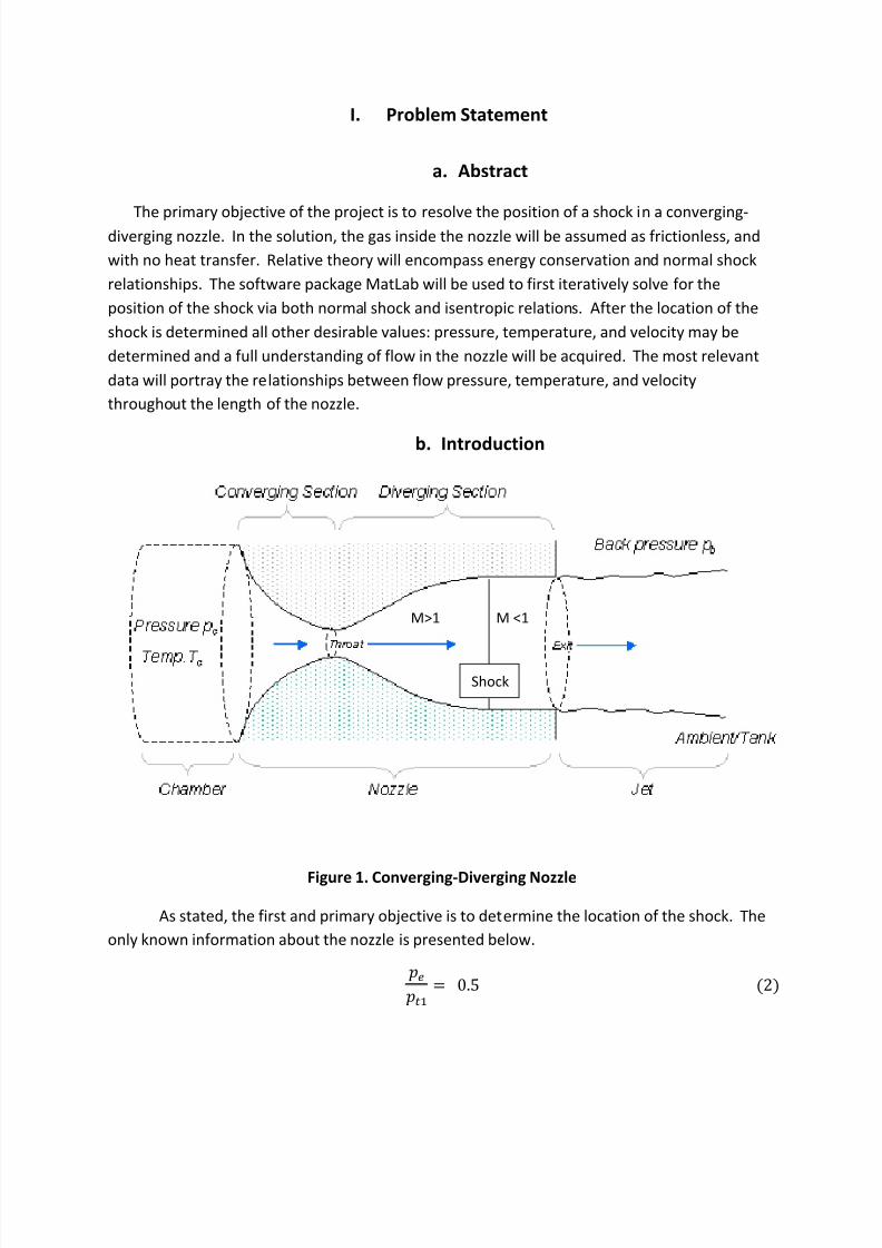
I. Problem Statement

a. Abstract

The primary objective of the project is to resolve the position of a shock in a converging-

diverging nozzle. In the solution, the gas inside the nozzle will be assumed as frictionless, and

with no heat transfer. Relative theory will encompass energy conservation and normal shock

relationships. The software package MatLab will be used to first iteratively solve for the

position of the shock via both normal shock and isentropic relations. After the location of the

shock is determined all other desirable values: pressure, temperature, and velocity may be

determined and a full understanding of flow in the nozzle will be acquired. The most relevant

data will portray the relationships between flow pressure, temperature, and velocity

throughout the length of the nozzle.

b. Introduction

Figure 1. Converging-Diverging Nozzle

As stated, the first and primary objective is to determine the location of the shock. The

only known information about the nozzle is presented below.

M <1M>1

Shock



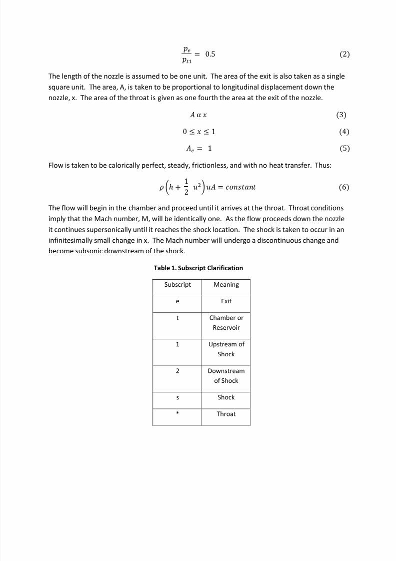
The length of the nozzle is assumed to be one unit. The area of the exit is also taken as a single

square unit. The area, A, is taken to be proportional to longitudinal displacement down the

nozzle, x. The area of the throat is given as one fourth the area at the exit of the nozzle.

Flow is taken to be calorically perfect, steady, frictionless, and with no heat transfer. Thus:

The flow will begin in the chamber and proceed until it arrives at the throat. Throat conditions

imply that the Mach number, M, will be identically one. As the flow proceeds down the nozzle

it continues supersonically until it reaches the shock location. The shock is taken to occur in an

infinitesimally small change in x. The Mach number will undergo a discontinuous change and

become subsonic downstream of the shock.

Table 1. Subscript Clarification

Subscript Meaning

e Exit

t Chamber or

Reservoir

1 Upstream of

Shock

2 Downstream

of Shock

s Shock

* Throat



II. Analysis

With the general trends of the flow in the nozzle described, a more in depth understanding

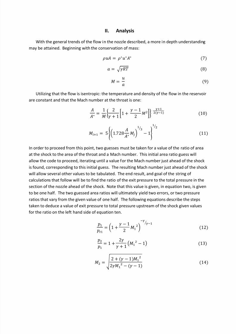
may be attained. Beginning with the conservation of mass:

Utilizing that the flow is isentropic: the temperature and density of the flow in the reservoir

are constant and that the Mach number at the throat is one:

In order to proceed from this point, two guesses must be taken for a value of the ratio of area

at the shock to the area of the throat and a Mach number. This initial area ratio guess will

allow the code to proceed, iterating until a value for the Mach number just ahead of the shock

is found, corresponding to this initial guess. The resulting Mach number just ahead of the shock

will allow several other values to be tabulated. The end result, and goal of the string of calculations that follow will be to find the ratio of the exit pressure to the total pressure in the

section of the nozzle ahead of the shock. Note that this value is given, in equation two, is given

to be one half. The two guessed area ratios will ultimately yield two errors, or two pressure

ratios that vary from the given value of one half. The following equations describe the steps

taken to deduce a value of exit pressure to total pressure upstream of the shock given values

for the ratio on the left hand side of equation ten.



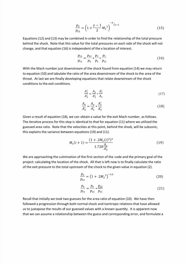
Equations (12) and (13) may be combined in order to find the relationship of the total pressure

behind the shock. Note that this value for the total pressures on each side of the shock will not

change, and that equation (16) is independent of the x location of interest.

With the Mach number just downstream of the shock found from equation (14) we may return

to equation (10) and tabulate the ratio of the area downstream of the shock to the area of the

throat. At last we are finally developing equations that relate downstream of the shock

conditions to the exit conditions.

Given a result of equation (18), we can obtain a value for the exit Mach number, as follows.

The iterative process for this step is identical to that for equation (11) where we utilized the

guessed area ratio. Note that the velocities at this point, behind the shock, will be subsonic;

this explains the variance between equations (19) and (11).

We are approaching the culmination of the first section of the code and the primary goal of the

project: calculating the location of the shock. All that is left now is to finally calculate the ratio

of the exit pressure to the total upstream of the shock to the given value in equation (2).

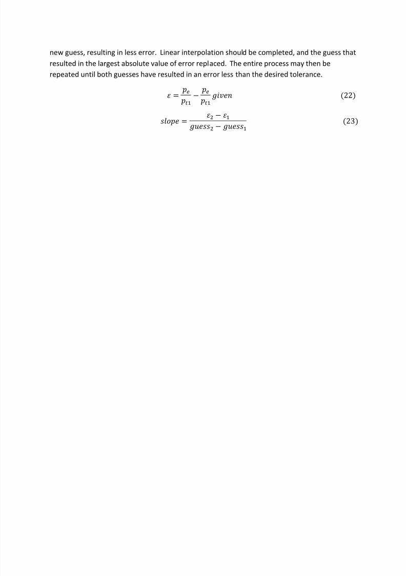
Recall that initially we took two guesses for the area ratio of equation (10). We have then

followed a progression through both normal shock and isentropic relations that have allowed

us to juxtapose the results of our guessed values with a known quantity. It is apparent now

that we can assume a relationship between the guess and corresponding error, and formulate a



new guess, resulting in less error. Linear interpolation should be completed, and the guess that

resulted in the largest absolute value of error replaced. The entire process may then be

repeated until both guesses have resulted in an error less than the desired tolerance.



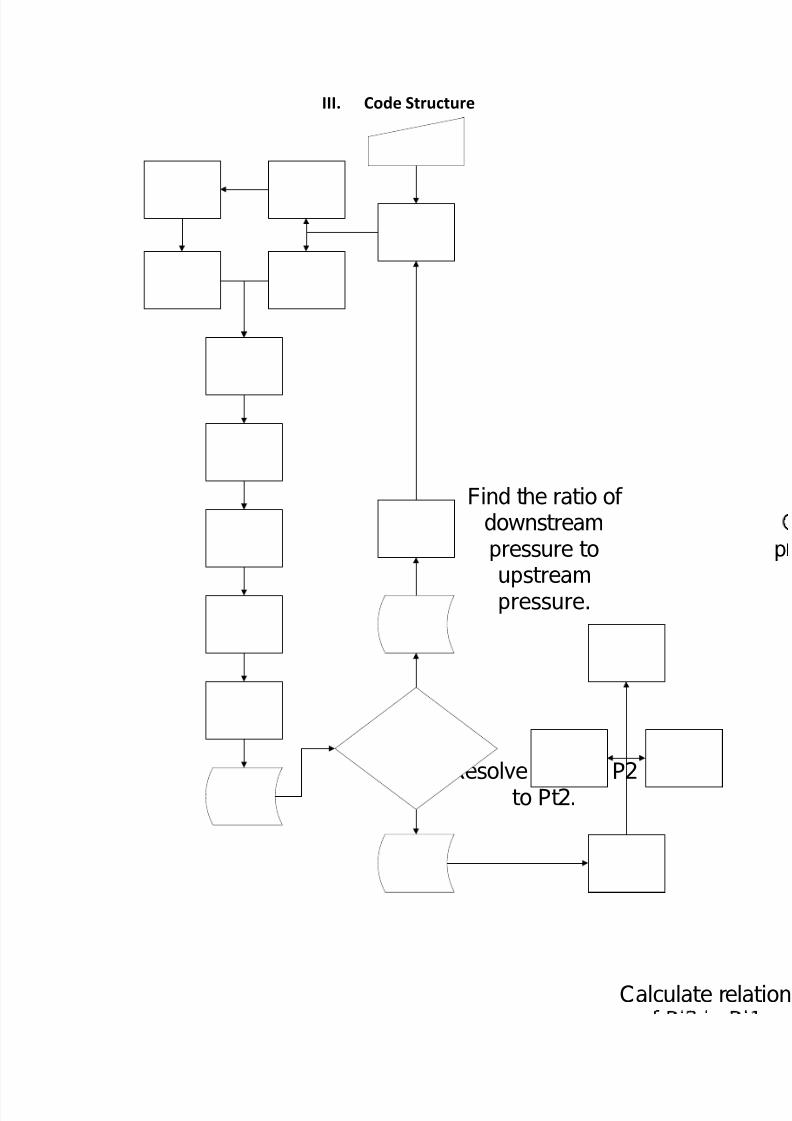
III. Code Structure

Find the ratio of downstreampressure to

upstreampressure.

Resolve ratio of P2to Pt2.

Calculate re



IV. Results and Discussion

a. Pressure vs. Position

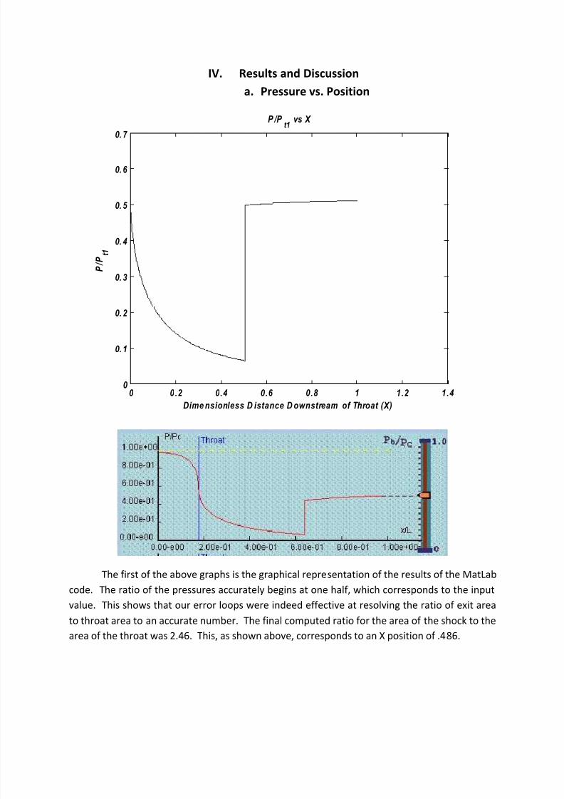
The first of the above graphs is the graphical representation of the results of the MatLab

code. The ratio of the pressures accurately begins at one half, which corresponds to the input

value. This shows that our error loops were indeed effective at resolving the ratio of exit area

to throat area to an accurate number. The final computed ratio for the area of the shock to the

area of the throat was 2.46. This, as shown above, corresponds to an X position of .486.

0 0.2 0.4 0.6 0.8 1 1.2 1.40

0. 1

0. 2

0. 3

0. 4

0. 5

0. 6

0. 7

Dime nsionless D istance D ownstream of Throat (X)

P / P t 1

P /P t1

vs X



T

he resultant figure of the MatLab code very closely resembles the plot made available byProfessor William Davenport of The Virginia Polytechnic Institute and State University. Both

graphs accurately depict the decay in pressure we would expect as a result of isentropic

relations. Keeping in mind that the total pressure remains the same and recalling from the

problem statement that the area varies linearly with X, it is inherent that the static pressure

must drop. The pressure then drastically increases via a discontinuity at the shock in order to

be able to meet the static pressure at the exit.



b. Temperature vs. Position

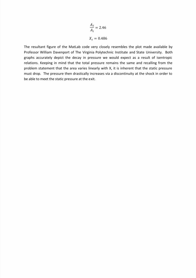
With the pressure distribution throughout the X domain behind us, analyzing the

temperature data is relatively simple. The two variables are related linearly via the ideal gas

law. The temperature begins at a value of approximately 0.8, appropriately decays so that the

ratio is less than one half by the time the flow reaches the shock point. At this location the

temperature abruptly increases, just as the pressure did. As the flow approaches the end of the

tunnel, and X values closer and closer to one, the temperature also increases to nearly one.

0 0.2 0.4 0.6 0.8 1 1.2 1.40.4

0.5

0.6

0.7

0.8

0.9

1

Di m

¡ ¢ ionless Distance Downstream of Throat (X)

T / T t 1

T/T t1

vs X



c. Mach Number vs. Position

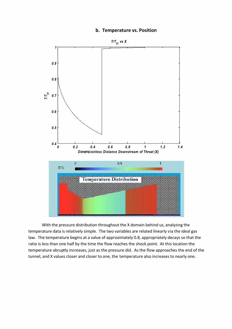
The Mach number vs X plot accurately begins at a Mach number equal to one where X is

zero, at the throat. The Mach number then begins to increase, as demonstrated in the

conservation of energy in equation (6). Due to the total enthalpy being conserved across a

shock, the total temperature is constant. The shock also converts some of the flows kinetic

energy into thermal energy; this may be noted in both the large jump in temperature at the

shock and inversely the decrease of Mach number at the shock.

0 0.2 0.4 0.6 0.8 1 1.2 1.40

0.5

1

1.5

2

2.5

Di mensionless Distance Downstream of Throat (X)

M a c h N u m b e r ( M )

Mach Number vs X



V. Code Appendix

VI. % Nathan Empson VII. %Aerospace 312- Project II VIII. %Converging-Diverging Nozzle Flow with a Shock IX. %Due: Friday April 24, 2009

X. XI. clc XII. clear

XIII. XIV. gamma = 1.4; XV. Ae=1; XVI. i=1;

XVII. j=1; XVIII. At=0.25; XIX. As=.25; XX. As2=1; XXI. M1(i) = 2;

XXII. M1_2(i) = 2; XXIII. Prat=0.5; XXIV. ErrTol=0.00001; XXV. Err2=1;

XXVI. Err1=1; XXVII. Me(j)=2; XXVIII. Me_2(j)=2; XXIX. XXX. %Large while loop, encompassing all normal shock and isentropic

equations XXXI. % that bring me to the pressure ratio. XXXII. while (abs(Err2)>ErrTol)

XXXIII. XXXIV. i=1; XXXV. %Iterating to find the first M1, given each of the two guesses. XXXVI. while(i<100) XXXVII. M1(i+1) = (5 * ((1.728* As/At* M1(i))^(1/3) - 1)) ^ (1/2); XXXVIII. M1_2(i+1) = (5 * ((1.728* As2/At* M1_2(i))^(1/3) - 1)) ^ (1/2); XXXIX. i=i+1;

XL. end XLI.

XLII. XLIII. P1_Pt1 = ((1 + (gamma - 1)/2 * M1(i)^2))^(-gamma/(gamma-1));

XLIV.

P1_Pt1_2 = ((1 + (gamma - 1)/2 * M1_2(i)^2))^(-gamma/(gamma-1)); XLV. XLVI. P2_P1 = 1 + 2*gamma/(gamma+1)* (M1(i)^2-1); XLVII. P2_P1_2 = 1 + 2*gamma/(gamma+1)* (M1_2(i)^2-1); XLVIII. XLIX. M2 = sqrt((1 + ((gamma - 1) /2 * M1(i)^2)) / ((gamma * M1(i)^2) -

(gamma - 1)/2));

L. M2_2 = sqrt((1 + ((gamma - 1) /2 * M1_2(i)^2)) / ((gamma *M1_2(i)^2) - (gamma - 1)/2));



LI. LII. P2_Pt2 = ( 1 + (gamma-1)/2 * M2^2)^ (-gamma/(gamma-1));

LIII. P2_Pt2_2 = ( 1 + (gamma-1)/2 * M2_2^2)^ (-gamma/(gamma-1)); LIV. LV. Pt2_Pt1 = P2_P1 * P1_Pt1 / P2_Pt2; LVI. Pt2_Pt1_2 = P2_P1_2 * P1_Pt1_2 / P2_Pt2_2;

LVII. LVIII. A2_A2t = 1/M2* ((1+0.2*M2^2))^3/ 1.728; LIX. A2_A2t_2 = 1/M2_2* ((1+0.2*M2_2^2))^3/ 1.728; LX. LXI. A2t_A1t = 2/ A2_A2t;

LXII. A2t_A1t_2 = 2/A2_A2t_2; LXIII. LXIV. Ae_A2t = Ae/At / A2t_A1t; LXV. Ae_A2t_2 = Ae/At / A2t_A1t_2;

LXVI. j=1; LXVII. %Iterating to find Me given the quatites calculted via the two

LXVIII. %current guesses. LXIX. while(j<100) LXX. Me(j+1) = (1 + 0.2 * Me(j)^2)^3/(1.728 * Ae_A2t); LXXI. Me_2(j+1) = (1 + 0.2 * Me_2(j)^2)^3/(1.728 * Ae_A2t_2); LXXII. j=j+1; LXXIII. end LXXIV. LXXV. Pe_Pt2 = (1 + 0.2 * Me(j)^2) ^(-3.5); LXXVI. Pe_Pt2_2 = (1 + 0.2 * Me_2(j)^2) ^(-3.5); LXXVII. LXXVIII. Pe_Pt1 = Pe_Pt2* Pt2_Pt1; LXXIX. Pe_Pt1_2 = Pe_Pt2_2* Pt2_Pt1_2;

LXXX. %The pressure ratios of exit to total are found. Compare this tothe

LXXXI. %given value, tabulate error, interpolate. LXXXII. Err1 = Pe_Pt1 - Prat; LXXXIII. Err2 = Pe_Pt1_2 - Prat; LXXXIV. LXXXV. slope = (Err2-Err1)/(As2-As); LXXXVI. yint= -slope* As + Err1; LXXXVII. NewAs = -yint/slope; LXXXVIII. %Following if loops replace the guess that causes the largest error. LXXXIX. %The loops are formulated so that only one error needs be checked

in the

XC. %total error loop. XCI. if (abs(Err2) < abs(Err1))

XCII. As = As2;

XCIII. As2=NewAs; XCIV. end XCV. if (abs(Err2) > abs (Err1))

XCVI. XCVII. As2=NewAs;



XCVIII. end XCIX. end

C. CI. k=1; CII. X(k)=0;

CIII. M(k) = 1; CIV. PPtot(k) = (1+(gamma-1)/2 *M(k)^2)^(-gamma/(gamma-1));

CV. T(k) = 1/(1+ (gamma-1)/2 * M(k)^2); CVI. A(k)=At; CVII. Xs = (As/At-1)/3; CVIII. inc=Xs/1000; CIX. Mitt(1)=2; CX.

CXI. while (X(k)<Xs) CXII. X(k+1)=X(k)+inc; %Getting arrays: 1 each for X pos. and Area. CXIII. A(k+1)= 3/4*X(k)+ At; CXIV. p=1;

CXV.

CXVI. %Iterates, finding a correct Mach number for each X or area ratio. CXVII. while(p<100) CXVIII. Mitt(p+1) = (5 * ((1.728* A(k)/At* Mitt(p))^(1/3) - 1)) ^ (1/2); CXIX. p=p+1; CXX. end CXXI. PPtot(k+1) = (1+(gamma-1)/2 *M(k)^2)^(-gamma/(gamma-1));

CXXII. M(k+1)=Mitt(p); %Plucks each of the M numbers after being iterated. CXXIII. T(k+1) = 1/(1+ (gamma-1)/2 * M(k)^2); CXXIV. CXXV. k=k+1; CXXVI. CXXVII. end CXXVIII. X(k+1)=X(k); CXXIX. M(k+1)=M2; CXXX. A(k+1)=A(k); CXXXI. PPtot(k+1) = PPtot(k); CXXXII. T(k+1) = T(k); CXXXIII. CXXXIV. while (X(k)<1) CXXXV. X(k+1)=X(k)+inc; CXXXVI. A(k+1)= 3/4*X(k)+ At; CXXXVII. p=1; CXXXVIII. CXXXIX. while(p<100)

CXL. Mitt(p+1) = (1 + 0.2 * Mitt(p) ^2 )^3/(1.728*(A(k)/At)); CXLI. p=p+1; CXLII. end CXLIII. CXLIV. PPtot(k+1) = (1+(gamma-1)/2 *M(k)^2)^(-gamma/(gamma-1))*Pt2_Pt1; CXLV. M(k+1)=Mitt(p); CXLVI. k=k+1;



CXLVII. T(k) = 1/(1+ (gamma-1)/2 * M(k)^2); CXLVIII. CXLIX.

CL. end CLI.

CLII. plot(X,M) CLIII. xlabel ('Dimensionless Distance Downstream of Throat (X)') CLIV. ylabel ('Mach Number (M)') CLV. title ('Mach Number vs X') CLVI. CLVII. % plot(X,PPtot) CLVIII. % xlabel ('Dimensionless Distance Downstream of Throat (X)') CLIX. % ylabel ('P/P_t_1') CLX. % title ('P/P_t_1 vs X') CLXI. CLXII. % plot(X,T) CLXIII. % xlabel ('Dimensionless Distance Downstream of Throat (X)')

CLXIV. % ylabel ('T/T_t_1') CLXV. % title ('T/T_t_1 vs X') CLXVI. CLXVII. CLXVIII. CLXIX. CLXX. CLXXI. CLXXII.

Aerospace 312 Proj 2

Documents

Transcript of Aerospace 312 Proj 2