A methodology for online rotor stress monitoring using ... · Green’s functions and Duhamel’s...

TRANSACTIONS OF THE INSTITUTE OF FLUID-FLOW MACHINERY

No. 133, 2016, 13–37

Mariusz Banaszkiewicza,b∗, Krzysztof Dominiczaka,b

A methodology for online rotor stress monitoringusing equivalent Green’s function and steam

temperature model

a GE Power sp. z o.o., Stoczniowa 2, 82-300 Elbląg, Polandb Institute of Fluid Flow Machinery, Polish Academy of Sciences,

80-231 Gdańsk, Fiszera 14, Poland

AbstractThe requirement of high operational flexibility of utility power plants creates a need of usingonline systems for monitoring and control of damage of critical components, e.g., steam turbinerotors. Such systems make use of different measurements and mathematical models enablingcalculation of thermal stresses and their continuous control. The paper presents key elements ofthe proposed system and discusses their use from the point of view of thermodynamics and heattransfer. Thermodynamic relationships, well proven in design calculations, were applied to cal-culate online the steam temperature at critical locations using standard turbine measurementsas input signals. The model predictions were compared with operational data from a real powerplant during a warm start-up and show reasonably good accuracy. The effect of variable heattransfer coefficient and material properties on thermal stresses was investigated numerically byfinite element method (FEM) on a cylinder model, and a concept of equivalent Green’s functionwas introduced to account for this variability in thermal stress model based on Duhamel’s inte-gral. This approach was shown to produce accurate results for more complicated geometries bycomparing thermal stresses at rotor blade groove computed using FEM and Duhamel’s integral.

Keywords: Steam turbine; Thermal stress; Green’s functions; Duhamel’s integral

∗Corresponding Author. Email adress: [email protected]

ISSN 0079-3205 Transactions IFFM 133(2016) 13–37

14 M. Banaszkiewicz and K. Dominiczak

Nomenclature

c0 – isentropic velocity, m/scp – specific heat, J/kg KE – Young modulus, MPaG – Green’s function for stress, MPa/◦Ch – enthalpy, kJ/kgm – mass flow rate, kg/sn – rotational speed, rev/minp – pressure, MPar – radial coordinate, mT – temperature, ◦Ct – time, su – circumferential velocity, m/sv – specific volume, m3/kgX – Green’s function for temperature, ◦C/◦Cy – valve opening, %

Greek symbols

α – heat transfer coefficient, W/m2Kβ – thermal expansion coefficient, 1/Kη – efficiencyλ – thermal conductivity, W/m Kν – Poisson numberσ – stress, MPa

Subscripts and superscripts

CS – control stageN – nozzleeq – equivalentT – throatm – metalperm – permissibles – steamsurf – surface0 – upstream stop valves1 – downstream stop valves2 – downstream control valvesVi – valve (i = 1, 2, 3, 4)

1 Introduction

Modern energy markets put a requirement of high operational flexibility of powerplant units [1,2]. Due to this, new designed units, including steam turbines, haveto fulfill a series of requirements regarding the number and rate of change of spec-ified operation states. With regard to steam turbines, the requirements concern


A methodology for online rotor stress monitoring using equivalent. . . 1515

the number and time of start-ups from different thermal conditions and the rateof load change. The above operation states generate elevated loads and stressesin turbine components leading to material damage due to thermomechanical fa-tigue [3].

The problem of thermal stress monitoring and control in steam turbines wasconsidered already at mid-sixties [4]. In the first thermal stress control systems,steam turbine rotors were supervised using start-up probes which were thermo-physical models of turbine rotors [5–7]. Thermal stresses were calculated basedon measured temperature difference between the probe surface and its integral-averaged temperature. A better accuracy of stress calculation was achieved byreplacing the measured average temperature with a mathematical model [8–10].Further development of thermal stress supervision systems consisted in completeresignation from the temperature probe and modeling thermal stresses based onthe standard process measurements of power units, which were a basis for calculat-ing the characteristic temperature difference surface-mean [11]. Rusin et al. [12]proposed a new method of thermal stress modeling in turbine rotors employingGreen’s functions and Duhamel’s integral, and steam temperature measurementat critical location. The Green’s functions and Duhamel’s integral have been formany years used for fatigue life monitoring of nuclear plants equipment by suchcompanies like EPRI [13–15], GE [16] or EDF [17–18]. Such an approach has alsobeen adopted for monitoring of power boilers operation by Taler et al. [19], andas shown by Lee et al. [20] can also be used for calculating stress intensity factorsat transient thermal loads. Recent developments in the field are focused on theuse of artificial neural networks for predicting boiler wall temperature [21] andturbine thermal stresses [22–23].

The major issue in using Green’s function and Duhamel’s integral methodin modeling transient thermal stresses in steam turbines components is time-dependence of material physical properties and heat transfer coefficients affectingproper evaluation of Green’s functions. There are known approaches assuming de-termination of the influence functions at constant values of these quantities [24].The inclusion of temperature dependent physical properties proposed by Koo etal. [25] relies on determining the weight functions for steady-state and transientoperating conditions. A more important, in most cases, variation of heat trans-fer coefficient can be taken into account by calculating the surface temperatureusing a reduced heat transfer model and employing Green’s function to calculatea stress response to the step change of metal surface temperature [26]. However,numerical solution of a multidimensional heat transfer model is complicated andtime-consuming, and due to this cannot be used in online calculations. A full in-



clusion of time variability of the physical properties and heat transfer coefficientsproposed by Zhang et al. [27] relies on the solution of nonlinear heat conductionproblem by using artificial parameter method and superposition rule and replac-ing the time-dependent heat transfer coefficient with a constant value togetherwith a modified fluid temperature. The effectiveness of the method has beenproved by an example of a three-dimensional model of a pressure vessel of nuclearreactor.

The present paper deals with the problems of modeling steam temperatureand thermal stresses for online supervision of low-cycle fatigue life. A controlsystem is proposed and its main elements are:

• thermodynamic model enabling fast calculation of steam temperature atcritical location,

• thermal stress model for online calculation of rotor thermal stresses.The models have been validated by comparing the results of numerical calculationswith real turbine measurements and more accurate 3D simulations.

2 Thermal stress control system

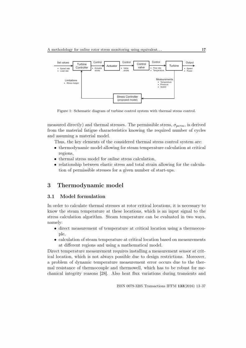
Thermal stress control systems of steam turbine rotors are currently a commonlyused measure of protecting the design fatigue life of high- and intermediate pres-sure turbine rotors. These systems are very important elements of turbine controland protection systems and operate in closed-loop control. A schematic diagramof turbine control system including a module responsible for thermal stress controlis shown in Fig. 1. Based on turbine measurements (e.g., temperature, pressure,speed), the stress controller calculates stresses and load fraction and outputs tothe turbine controller a signal of stress margin which reduces the set values ofspeed or load rates. The turbine controller positions, with the help of actuator,the control valve head controlling in this way the steam flow rate and temperatureupstream the turbine blading. These two parameters have impact on the rotortemperature and the resulting thermal stresses.

The thermal stress controller calculates stresses at rotor critical locations onthe basis of measurement signals and compares them with the permissible stresses.On the basis of these two stresses, a load fraction, LF, is calculated using theformula

LF =σeqσperm

. (1)

The equivalent stress, σeq, is computed based on the measured temperature, pres-sure, rotational speed and using a mathematical model of temperature (if it is not



Output

? Speed

? Power

Control

? Flow rate

? Temperature

Control

? Valvestroke

Control

? Actuatorstroke

Set values

? Speed rate

? Load rate

TurbineController

Turbine

Stress Controller(proposed model)

Limitations? Stress margin

Measurements? Temperature

? Pressure

? Speed

ActuatorControlvalve

Figure 1: Schematic diagram of turbine control system with thermal stress control.

measured directly) and thermal stresses. The permissible stress, σperm, is derivedfrom the material fatigue characteristics knowing the required number of cyclesand assuming a material model.

Thus, the key elements of the considered thermal stress control system are:• thermodynamic model allowing for steam temperature calculation at critical

regions,• thermal stress model for online stress calculation,• relationship between elastic stress and total strain allowing for the calcula-

tion of permissible stresses for a given number of start-ups.

3 Thermodynamic model

3.1 Model formulation

In order to calculate thermal stresses at rotor critical locations, it is necessary toknow the steam temperature at these locations, which is an input signal to thestress calculation algorithm. Steam temperature can be evaluated in two ways,namely:

• direct measurement of temperature at critical location using a thermocou-ple,

• calculation of steam temperature at critical location based on measurementsat different regions and using a mathematical model.

Direct temperature measurement requires installing a measurement sensor at crit-ical location, which is not always possible due to design restrictions. Moreover,a problem of dynamic temperature measurement error occurs due to the ther-mal resistance of thermocouple and thermowell, which has to be robust for me-chanical integrity reasons [28]. Also heat flux variations during transients and



high-frequency unsteadiness occurring at every rotor passage with varying am-plitudes originating from complex blade row interactions make the heat transfertime-dependent and accurate measurements become essential for correct thermalassessment of steam turbines [29].

A more universal way is steam temperature calculation at critical locationbased on a measurement at a different suitable point. For this purpose, a math-ematical model is required describing steam thermodynamic process from themeasurement point to the critical location. In online monitoring and control sys-tems, the thermodynamic model should be fast, accurate and reliable, to ensurethe capability of its implementation in the turbine control system and the re-quired quality of computations. For this reason, only zero- or one-dimensionalmodels with a minimum number of iteration loops can be considered. Modelingsteam temperature is the only way of its evaluation in the areas not accessiblefor measurement or in turbines not equipped with the required temperature mea-surement.

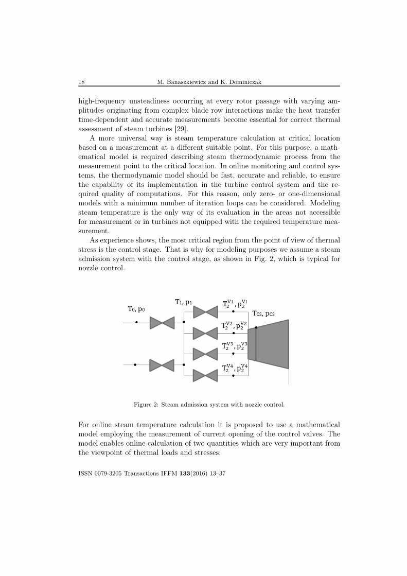
As experience shows, the most critical region from the point of view of thermalstress is the control stage. That is why for modeling purposes we assume a steamadmission system with the control stage, as shown in Fig. 2, which is typical fornozzle control.

Figure 2: Steam admission system with nozzle control.

For online steam temperature calculation it is proposed to use a mathematicalmodel employing the measurement of current opening of the control valves. Themodel enables online calculation of two quantities which are very important fromthe viewpoint of thermal loads and stresses:



• steam temperature in control stage chamber and temperatures downstreameach control valve and nozzle sector for current openings,

• mass flow rates through each valve and total mass flow through the turbine.For the considered steam admission system consisting of two stop valves and fourcontrol valves, the following measurements are used as input signals to the steamtemperature model:

• live steam temperature – T0,• live steam pressure – p0,• steam pressure downstream control stage – pCS,• control valves openings – yV 1, yV 2, yV 3 and yV 4,• turboset rotational speed n.The steam temperature model is based on the relations known from steam

turbines theory and used in design calculations. In the proposed mathematicalmodel these relationships are given in a consistent way with necessary simplifi-cations and additional elements resulting from the specifity of online calculationscarried out in the entire range of turbine operating conditions. In the first step,steam pressures downstream control valves and mass flow rates through each noz-zle sector are calculated. One control valve cooperates in series with a nozzlesector. For such a system, the condition of equal mass flow rates can be written

m2 = mD . (2)

The valve mass flow rate m2 is given by the relationship [30]:

m2 = 0.667qAT

√p1v1

, (3)

where q is a relative mass flow rate determined from the valve characteristics ina function of opening and pressure ratio, AT – section area of valve throat, whilep1 and v1 denote steam pressure and specific volume upstream the valve. Thenozzle sector mass flow rate mD is described by equation [31]

mN = 1.42p2 (p0v0)−0.5AN

√−0.09 + 1.09pCS/p2 − (pCS/p2)

2 , (4)

where AN is exit section area of nozzle sector.A nonlinear equation with unknown p2 is obtained from Eqs. (2)–(4) and is

solved iteratively using the bisection method. Knowing the pressure p2, we cancalculate the mass flow rate from Eq. (3) or (4). Performing similar calculationsfor each valve, we find the appropriate pressures and mass flow rates for all valvesand nozzle sectors.



In the control valves, isenthalpic process of steam throttling from upstreampressure, p1, to downstream pressure, p2, takes place. Assuming additionally thatthe enthalpy upstream the control valve is equal to the steam enthalpy upstreamthe stop valve, we can express steam temperature downstream the control valves asa function of steam temperature and pressures directly measured on the turbine:

T2 = f(p0, T0, p2) . (5)

Knowing the steam temperature and pressure downstream the control valves andsteam pressure downstream the control stage, we can calculate steam enthalpyusing the formula known from the theory of steam turbines [31]

hCS =h1CSm

V 12 + h2CSm

V 22 + h3CSm

V 32 + h4CSm

V 42

mV 12 + mV 2

2 + mV 32 + mV 4

2

, (6)

where: h1CS , h2CS , h3CS , h4CS – steam enthalpies behind each sector of the controlstage.

These enthalpies depend on the circumferential efficiency, η0, of each sectorwhich depends on the current opening of the control valve feeding this sector. Inthis way, in the proposed calculation model a relationship between the controlstage efficiency and current valve openings is considered. It provides a capabilityto take into account in online calculations the influence of valve timing on steamtemperature in the control stage.

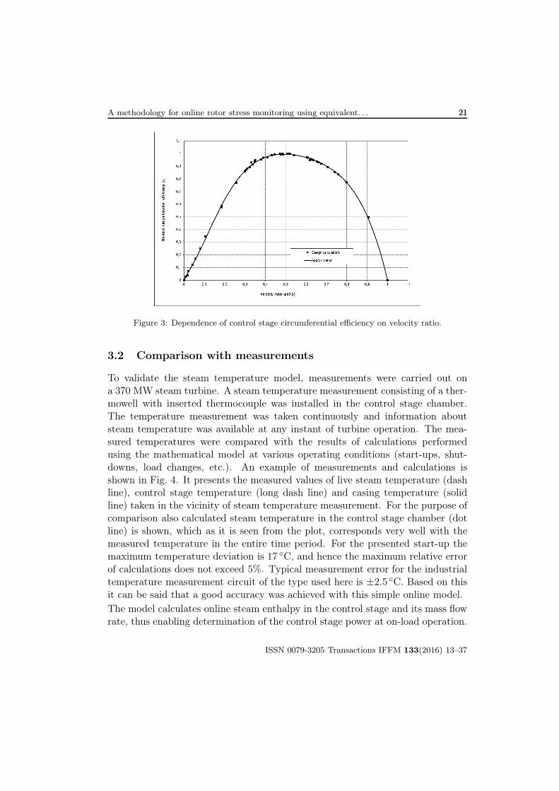
The circumferential efficiency is a function of velocity ratio u/c0 and for on-line calculations, an individual efficiency characteristics prepared on the basis ofcontrol stage calculations using design tool is used. An example of stage efficiencycharacteristics is shown in Fig. 3. The results of calculations performed with thedesign code are presented by squares, while the continuous line represents anapproximation with the function

ηo = A+B

(u

c0

)+ C

(u

c0

)ln

(u

c0

)+D

(u

c0

)2

+

E

(u

c0

)2

ln

(u

c0

)+ F

(u

c0

)2.5

+G exp

(− u

c0

)(7)

in which A, B, C . . .G are the coefficients of the approximation function. In thisfigure the values of stage efficiency are related to its maximum value.

The calculated steam enthalpy, hCS , and measured pressure in the controlstage, pCS , allow to determine steam temperature from a thermodynamic func-tion:

TCS = f(pCS, hCS) . (8)



Figure 3: Dependence of control stage circumferential efficiency on velocity ratio.

3.2 Comparison with measurements

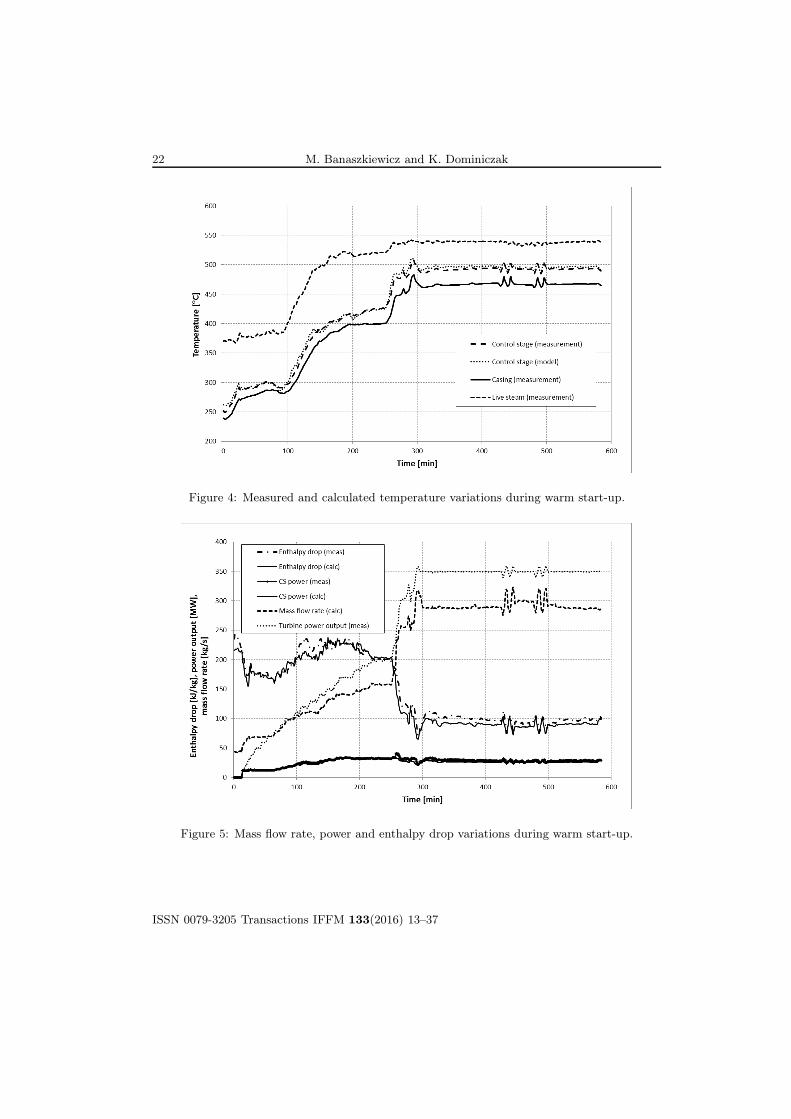
To validate the steam temperature model, measurements were carried out ona 370 MW steam turbine. A steam temperature measurement consisting of a ther-mowell with inserted thermocouple was installed in the control stage chamber.The temperature measurement was taken continuously and information aboutsteam temperature was available at any instant of turbine operation. The mea-sured temperatures were compared with the results of calculations performedusing the mathematical model at various operating conditions (start-ups, shut-downs, load changes, etc.). An example of measurements and calculations isshown in Fig. 4. It presents the measured values of live steam temperature (dashline), control stage temperature (long dash line) and casing temperature (solidline) taken in the vicinity of steam temperature measurement. For the purpose ofcomparison also calculated steam temperature in the control stage chamber (dotline) is shown, which as it is seen from the plot, corresponds very well with themeasured temperature in the entire time period. For the presented start-up themaximum temperature deviation is 17 ◦C, and hence the maximum relative errorof calculations does not exceed 5%. Typical measurement error for the industrialtemperature measurement circuit of the type used here is ±2.5 ◦C. Based on thisit can be said that a good accuracy was achieved with this simple online model.The model calculates online steam enthalpy in the control stage and its mass flowrate, thus enabling determination of the control stage power at on-load operation.



Figure 4: Measured and calculated temperature variations during warm start-up.

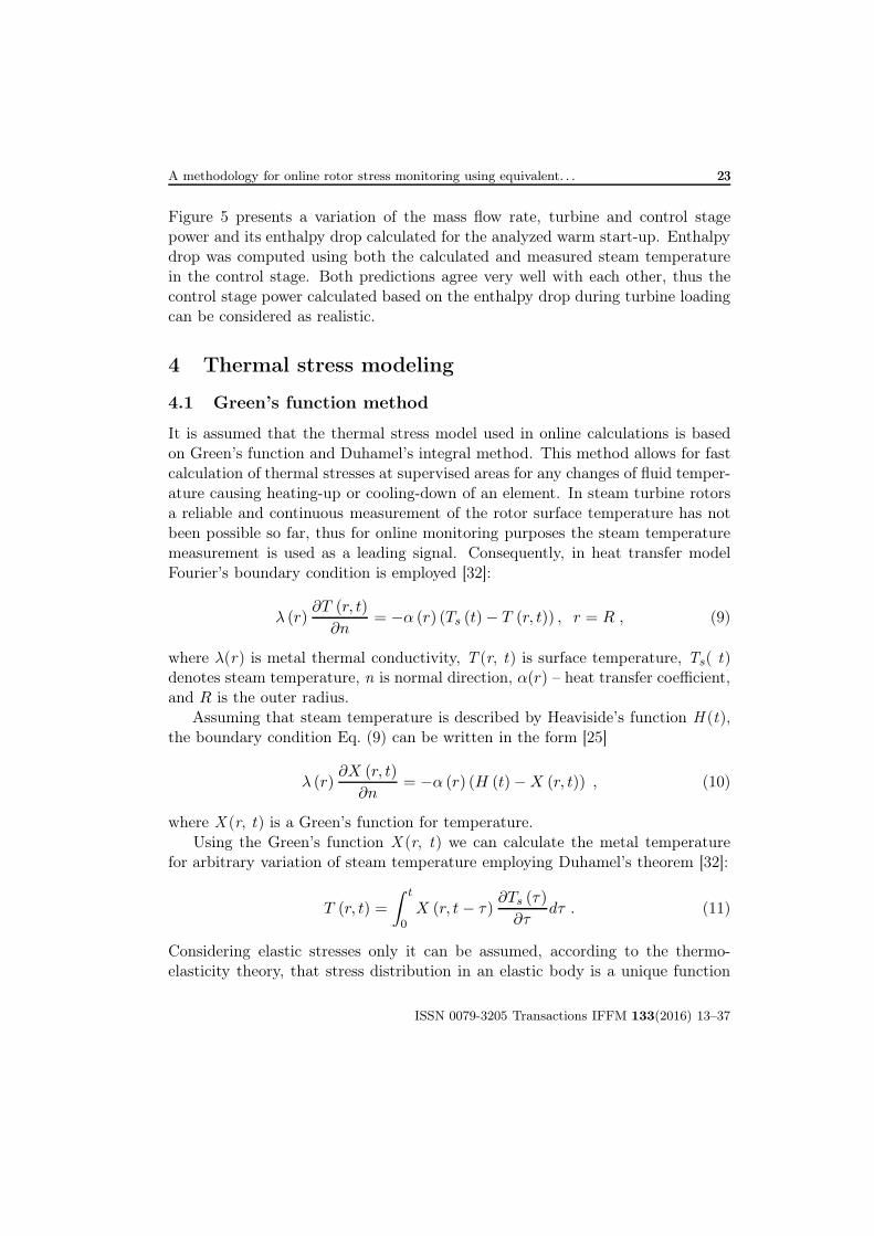
Figure 5: Mass flow rate, power and enthalpy drop variations during warm start-up.



Figure 5 presents a variation of the mass flow rate, turbine and control stagepower and its enthalpy drop calculated for the analyzed warm start-up. Enthalpydrop was computed using both the calculated and measured steam temperaturein the control stage. Both predictions agree very well with each other, thus thecontrol stage power calculated based on the enthalpy drop during turbine loadingcan be considered as realistic.

4 Thermal stress modeling

4.1 Green’s function method

It is assumed that the thermal stress model used in online calculations is basedon Green’s function and Duhamel’s integral method. This method allows for fastcalculation of thermal stresses at supervised areas for any changes of fluid temper-ature causing heating-up or cooling-down of an element. In steam turbine rotorsa reliable and continuous measurement of the rotor surface temperature has notbeen possible so far, thus for online monitoring purposes the steam temperaturemeasurement is used as a leading signal. Consequently, in heat transfer modelFourier’s boundary condition is employed [32]:

λ (r)∂T (r, t)

∂n= −α (r) (Ts (t)− T (r, t)) , r = R , (9)

where λ(r) is metal thermal conductivity, T (r, t) is surface temperature, Ts( t)denotes steam temperature, n is normal direction, α(r) – heat transfer coefficient,and R is the outer radius.

Assuming that steam temperature is described by Heaviside’s function H (t),the boundary condition Eq. (9) can be written in the form [25]

λ (r)∂X (r, t)

∂n= −α (r) (H (t)−X (r, t)) , (10)

where X (r, t) is a Green’s function for temperature.Using the Green’s function X (r, t) we can calculate the metal temperature

for arbitrary variation of steam temperature employing Duhamel’s theorem [32]:

T (r, t) =

∫ t

0X (r, t− τ)

∂Ts (τ)

∂τdτ . (11)

Considering elastic stresses only it can be assumed, according to the thermo-elasticity theory, that stress distribution in an elastic body is a unique function



of temperature distribution, and in this connection the thermal stresses can becalculated using Duhamel’s integral as

σij (r, t) =

∫ t

0Gij (r, t− τ)

∂Ts (τ)

∂τdτ , (12)

where Gij(r, t) is a Green’s function for thermal stress component ij.For simple geometries (plate, cylinder, sphere) Green’s functions for temper-

ature and stress can be determined analytically by solving one-dimensional tran-sient heat conduction problem. In case of more complicated shapes it is necessaryto use numerical methods, e.g., finite element method. Also in our case numericalintegration of Eq. (12) is necessary, it is thus transformed from continuous intodiscrete form

σij (r, t) = Gs,ij (r)Ts (t) +t∑

t−td

Gt,ij (r, t− τ)∆Ts (τ) , (13)

where td is a cut-off time, Gs,ij(r) is a value of the influence function in steadystate, while Gt,ij(r) is a transient part of the influence function.

Green’s functions are determined individually for each supervised region, andin case of thermal stresses these functions must be determined for each componentof the stress tensor σij .

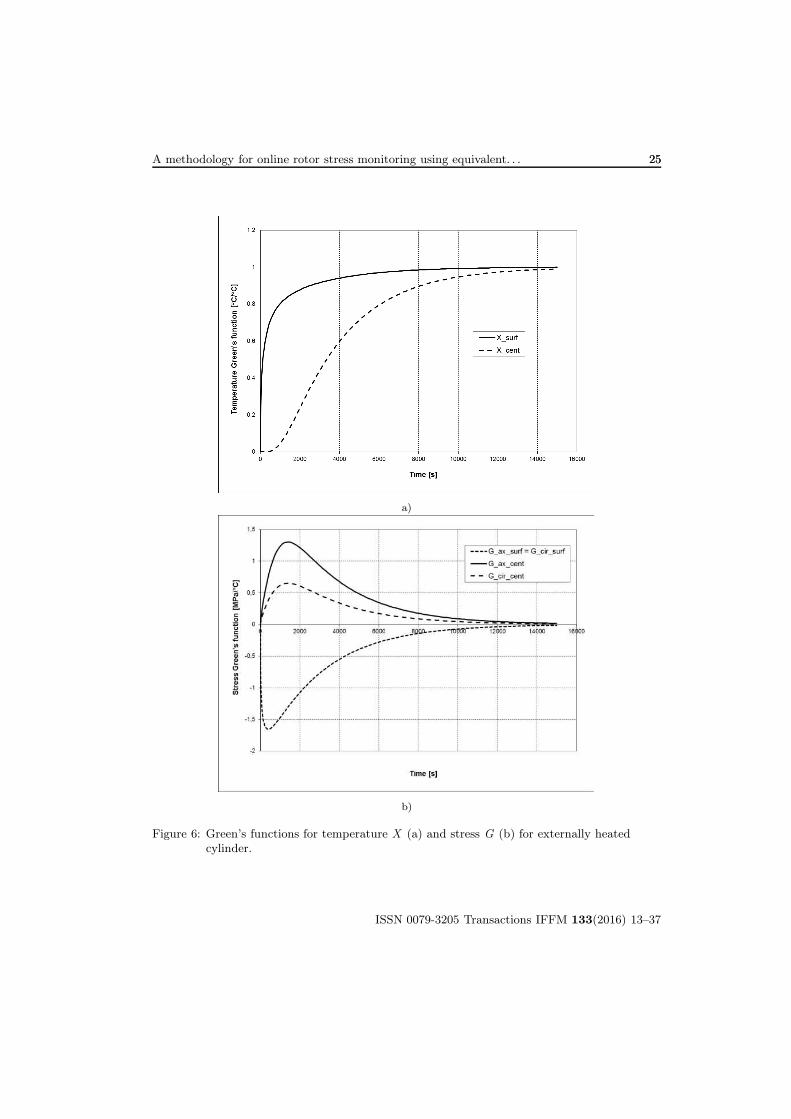
An example of Green’s function for temperature and stress components atstep increase of fluid temperature by 1 ◦C heating the external surface of a longcylinder is shown in Fig. 6. The calculations were performed with constant heattransfer coefficient α = 1000 W/m2/K and constant material physical propertiesevaluated at temperature 350 ◦C. The temperature (Fig. 6a) and stress (Fig. 6b)responses are presented for the cylinder axis and its outer surface heated by steam.

The Green’s function for surface temperature, X_surf, initially rapidly in-creases and reaches nearly 1 after approx. 104 s. The temperature at cylinderaxis, X_cent, shows some inercy and a delay time of temperature response equal500 s is seen. After this time the temperature increases at approximately constantrate and after about 4000 s the rate of variation visibly starts to decrease. Thecylinder surface response is typical for surface-type sensor, while Green’s functionat cylinder axis is a response of middle-type sensor. The stress response at bothareas is a result of temperature variations: axial and circumferential stresses atcylinder surface are equal to each other and rapidly grow reaching a minimum(compressive stress) and subsequently tend slowly to zero; the stresses at cylin-der axis grow more slowly, their maxima are lower than at surface (axial stressis two times higher than circumferential stress) and are tensile stresses (sign +).



a)

b)

Figure 6: Green’s functions for temperature X (a) and stress G (b) for externally heatedcylinder.



All stress components within the cylinder tend to zero and a stress-free state isreached after approx. 1.4×104 s, which corresponds to the instant when temper-ature within the whole cylinder is uniform.

4.2 Green’s function for temperature dependent materialproperties and time dependent heat transfer coefficient

The presented in the previous section Green’s functions for temperature X andthermal stresses G were determined with constant physical properties and con-stant heat transfer coefficient α. The physical properties of steel influencing tem-perature (specific heat, cp, thermal conductivity, λ) and stress (Young’s modulus,E, Poisson’s number, ν, thermal expansion coefficient, β) distribution stronglydepend on temperature, while heat transfer coefficient α varies with temperatureand flow velocity (via the Reynolds number Re). The dependence of these coef-ficients on temperature and velocity for typical operating conditions of 1CrMoVrotor is shown in Figs. 7 and 8. The heat transfer coefficient in labyrinth seal wascalculated using Kapinos et al. correlation [33]:

α · dλ

= 1.125Re0.65(δ

h

)0.35 (hs

)0.1 (bs

)0.32

, (14)

where d is the shaft diameter, δ is seal radial clearance, h is seal channel height,s is the distance between teeth, and b is the teeth width.

Among the considered physical properties the most varying is the specific heatwhich in the analysed temperature range increases by more than 50%. The largestdrop is observed for the Young’s modulus which decreases by more than 30%.Heat transfer coefficient depends most on the flow velocity. From the variation oflabyrinth seal, a, shown in Fig. 8 it is seen that its value can change even by anorder of magnitude. The influence of temperature is smaller and more distinct inthe range of higher velocities.

A consequence of the above shown variation of physical properties and heattransfer coefficient is a dependence of Green’s function, G, on these parameters.The dependence is illustrated in Fig. 9 showing Green’s function variations foraxial stress at cylinder surface calculated by finite element method at differenttemperatures and heat transfer coefficients. Each individual curve correspondsto stress variation determined at constant temperature, T = const, and constantheat transfer coefficient, α = const. The variation range of these parameters wasassumed so as to cover typical operating conditions of 1CrMoV rotors. As it isseen from the plots, the largest effect on the Green’s function G is observed forthe heat transfer coefficient, which significantly affects the stress maxima, time of



Figure 7: Dependence of typical physical properties of 1CrMoV rotor steel on temperature.

Figure 8: Dependence of heat transfer coefficient on temperature and velocity, accor. Eq.(14).



their occurrence and decay rate. The influence of temperature variation is muchsmaller and most visible from the instant of maximum stress to the moment oftheir vanishing.

Figure 9: Green’s function, G, for axial stress at cylinder surface at various temperatures andheat transfer coefficients.

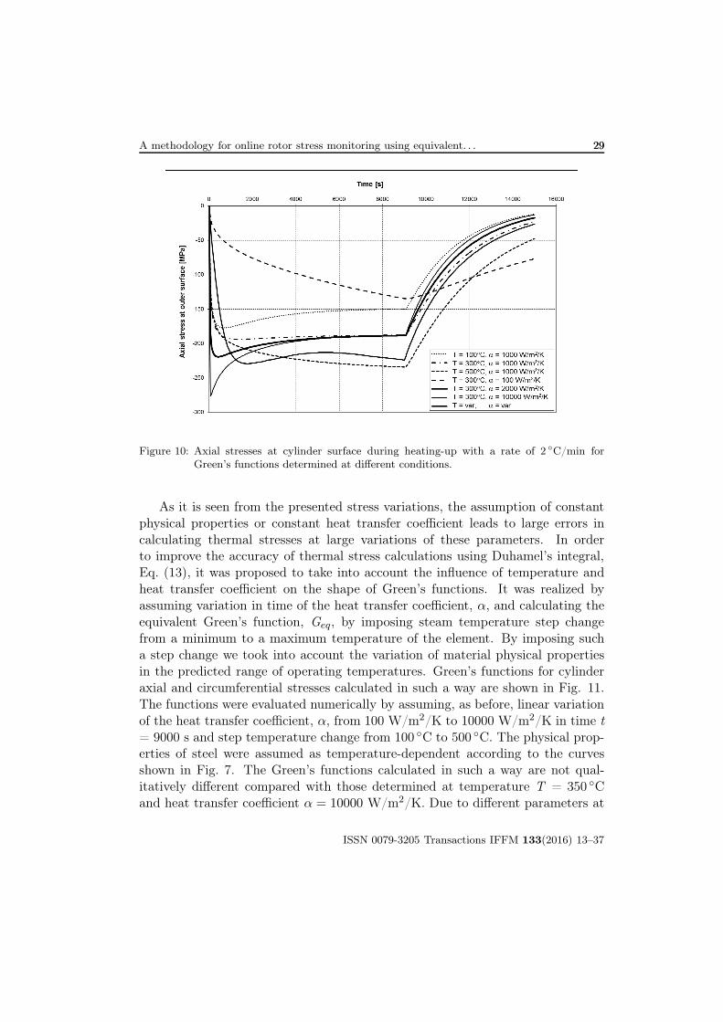
As a result of so high sensitivity of Green’s function, G, to the conditions atwhich it was determined, a scatter in stress variation calculated using Eq. (13)with different Green’s function is observed. Figure 10 presents axial stress vari-ation with time for cylinder surface calculated using the functions presented inFig. 9. The calculations were performed for the following conditions:

initial conditions: metal temperature Tm(0) = 100 ◦Csteam temperature Ts(0) = 200 ◦C

boundary condition: steam temperature rate dTs/dt = 2 ◦C/min

For comparison, also the axial stress variation calculated in three dimensionalheat transfer model with the same initial and boundary conditions but with heattransfer coefficient, a, linearly changing with time from 100 to 10000 W/m2/K isshown. The heat transfer coefficient was varied until t = 9000 s and from thisinstant remained constant.



Figure 10: Axial stresses at cylinder surface during heating-up with a rate of 2 ◦C/min forGreen’s functions determined at different conditions.

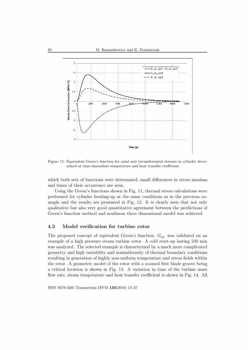
As it is seen from the presented stress variations, the assumption of constantphysical properties or constant heat transfer coefficient leads to large errors incalculating thermal stresses at large variations of these parameters. In orderto improve the accuracy of thermal stress calculations using Duhamel’s integral,Eq. (13), it was proposed to take into account the influence of temperature andheat transfer coefficient on the shape of Green’s functions. It was realized byassuming variation in time of the heat transfer coefficient, α, and calculating theequivalent Green’s function, Geq, by imposing steam temperature step changefrom a minimum to a maximum temperature of the element. By imposing sucha step change we took into account the variation of material physical propertiesin the predicted range of operating temperatures. Green’s functions for cylinderaxial and circumferential stresses calculated in such a way are shown in Fig. 11.The functions were evaluated numerically by assuming, as before, linear variationof the heat transfer coefficient, α, from 100 W/m2/K to 10000 W/m2/K in time t= 9000 s and step temperature change from 100 ◦C to 500 ◦C. The physical prop-erties of steel were assumed as temperature-dependent according to the curvesshown in Fig. 7. The Green’s functions calculated in such a way are not qual-itatively different compared with those determined at temperature T = 350 ◦Cand heat transfer coefficient α = 10000 W/m2/K. Due to different parameters at



Figure 11: Equivalent Green’s function for axial and circumferential stresses in cylinder deter-mined at time-dependent temperature and heat transfer coefficient.

which both sets of functions were determined, small differences in stress maximaand times of their occurrence are seen.

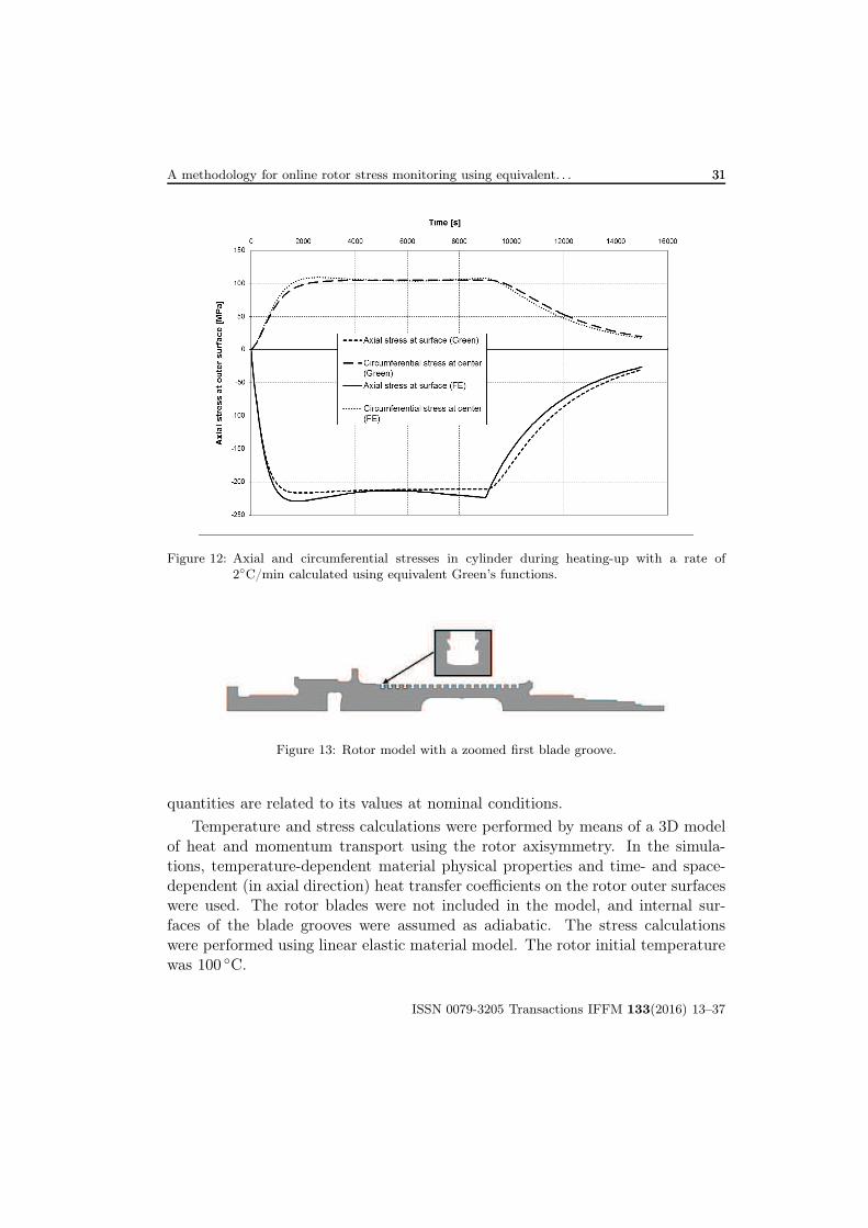
Using the Green’s functions shown in Fig. 11, thermal stress calculations wereperformed for cylinder heating-up at the same conditions as in the previous ex-ample and the results are presented in Fig. 12. It is clearly seen that not onlyqualitative but also very good quantitative agreement between the predictions ofGreen’s function method and nonlinear three dimensional model was achieved.

4.3 Model verification for turbine rotor

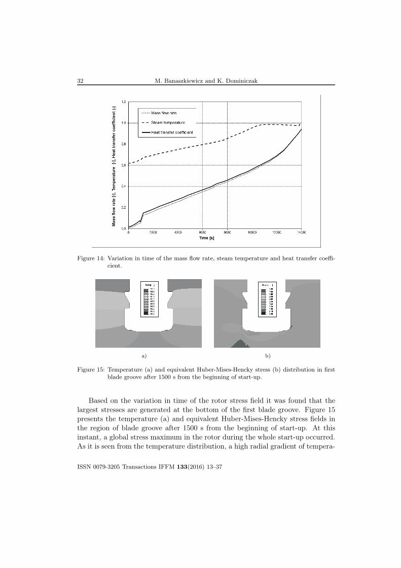
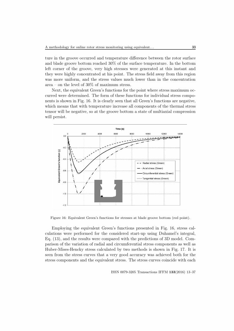
The proposed concept of equivalent Green’s function, Geq, was validated on anexample of a high pressure steam turbine rotor. A cold start-up lasting 240 minwas analyzed. The selected example is characterized by a much more complicatedgeometry and high variability and nonuniformity of thermal boundary conditionsresulting in generation of highly non-uniform temperature and stress fields withinthe rotor. A geometric model of the rotor with a zoomed first blade groove beinga critical location is shown in Fig. 13. A variation in time of the turbine massflow rate, steam temperature and heat transfer coefficient is shown in Fig. 14. All



Figure 12: Axial and circumferential stresses in cylinder during heating-up with a rate of2◦C/min calculated using equivalent Green’s functions.

Figure 13: Rotor model with a zoomed first blade groove.

quantities are related to its values at nominal conditions.

Temperature and stress calculations were performed by means of a 3D modelof heat and momentum transport using the rotor axisymmetry. In the simula-tions, temperature-dependent material physical properties and time- and space-dependent (in axial direction) heat transfer coefficients on the rotor outer surfaceswere used. The rotor blades were not included in the model, and internal sur-faces of the blade grooves were assumed as adiabatic. The stress calculationswere performed using linear elastic material model. The rotor initial temperaturewas 100 ◦C.



Figure 14: Variation in time of the mass flow rate, steam temperature and heat transfer coeffi-cient.

a) b)

Figure 15: Temperature (a) and equivalent Huber-Mises-Hencky stress (b) distribution in firstblade groove after 1500 s from the beginning of start-up.

Based on the variation in time of the rotor stress field it was found that thelargest stresses are generated at the bottom of the first blade groove. Figure 15presents the temperature (a) and equivalent Huber-Mises-Hencky stress fields inthe region of blade groove after 1500 s from the beginning of start-up. At thisinstant, a global stress maximum in the rotor during the whole start-up occurred.As it is seen from the temperature distribution, a high radial gradient of tempera-



ture in the groove occurred and temperature difference between the rotor surfaceand blade groove bottom reached 30% of the surface temperature. In the bottomleft corner of the groove, very high stresses were generated at this instant andthey were highly concentrated at his point. The stress field away from this regionwas more uniform, and the stress values much lower than in the concentrationarea – on the level of 30% of maximum stress.

Next, the equivalent Green’s functions for the point where stress maximum oc-curred were determined. The form of these functions for individual stress compo-nents is shown in Fig. 16. It is clearly seen that all Green’s functions are negative,which means that with temperature increase all components of the thermal stresstensor will be negative, so at the groove bottom a state of multiaxial compressionwill persist.

Figure 16: Equivalent Green’s functions for stresses at blade groove bottom (red point).

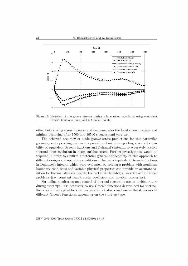
Employing the equivalent Green’s functions presented in Fig. 16, stress cal-culations were performed for the considered start-up using Duhamel’s integral,Eq. (13), and the results were compared with the predictions of 3D model. Com-parison of the variation of radial and circumferential stress components as well asHuber-Mises-Hencky stress calculated by two methods is shown in Fig. 17. It isseen from the stress curves that a very good accuracy was achieved both for thestress components and the equivalent stress. The stress curves coincide with each



Figure 17: Variation of the groove stresses during cold start-up calculated using equivalentGreen’s functions (lines) and 3D model (points).

other both during stress increase and decrease; also the local stress maxima andminima occurring after 1500 and 10500 s correspond very well.

The achieved accuracy of blade groove stress predictions for this particulargeometry and operating parameters provides a basis for expecting a general capa-bility of equivalent Green’s functions and Duhamel’s integral to accurately predictthermal stress evolution in steam turbine rotors. Further investigations would berequired in order to confirm a potential general applicability of this approach todifferent designs and operating conditions. The use of equivalent Geens’s functionsin Duhamel’s integral which were evaluated by solving a problem with nonlinearboundary conditions and variable physical properties can provide an accurate so-lution for thermal stresses, despite the fact that the integral was derived for linearproblems (i.e., constant heat transfer coefficient and physical properties).

For online monitoring and control of thermal stresses in steam turbine rotorsduring start-ups, it is necessary to use Green’s functions determined for thermo-flow conditions typical for cold, warm and hot starts and use in the stress modeldifferent Green’s functions, depending on the start-up type.



5 Conclusions

The paper presented a methodology of online thermal stress calculation and con-trol in steam turbine rotors. The main elements of the proposed methodologyare: thermodynamic model allowing for calculating steam temperature at criticallocations and rotor thermal stress model.

For calculating thermal stresses, steam temperature is used as a leading inputsignal which is calculated on the basis of thermodynamic model of the turbineinlet part. In such a case, it is not necessary to install a steam temperature mea-surement as the model is based on the turbo-set standard measurements. A modelof the control stage with four nozzle sectors capable of calculating transient steamtemperature downstream the stage for arbitrary openings of the control valves isstudied. Steam temperature measurements carried out during turbine transientoperating conditions and presented here for a warm start-up showed a potentialaccuracy of the investigated model.

In the rotor thermal stress model, Green’s function and Duhamel’s integralare used. A crucial effect of the variation of material physical properties andheat transfer coefficient on the shape of Green’s function and thermal stress evo-lution was shown on the example of a simple cylinder representing turbine rotorheated at constant rate. In order to take into account these variations the so-called equivalent Green’s function was proposed, which provides a potential foraccurate calculation of thermal stresses both for simple geometries and temper-ature changes (heating-up of cylinder), and for more complicated shapes of realsteam turbine rotors (e.g., blade grooves). However, it’s general applicability tosteam turbine rotors should be confirmed by further investigations. The equiva-lent Green’s functions are valid for given in advance thermo-flow conditions andtheir applicability to turbines’ start-ups is possible thanks to the exact definitionat design phase of start-up types and conditions at which they occur.

Received in July 2016

References

[1] Vogt J., Schaaf T., Helbig K.: Optimizing lifetime consumption and increasing flexibilityusing enhanced lifetime assessment methods with automated stress calculation from long-term operation data. In: Proc. ASME Turbo Expo 2013, San Antonio, June 03–07, 2013,GT2013-95068.

[2] Starkloff R., Alobaid F., Karner K., Epple B., Schmitz M., Boehm F.: Development andvalidation of a dynamic simulation model for a large coal-fired power plant. Appl. Therm.Eng. 91(2015), 496–506.



[3] Otterlee T., Lindsay G.: Using finite element analysis and thermal stress monitoring tomanage turbine defects without mechanical intervention. Joint Power Generation Confer-ence 3(1995), 295–299.

[4] Pahl G., Reitze W., Salm M.: Monitoring temperature changes in steam turbines. TheBrown Boveri Rev. 51(1964), 3, 165–175.

[5] Busse L.: Anfahrsonde. BBC-Studie HTGD51147, 1973.

[6] Dawson R.: Monitoring and control of thermal stresses and component life expenditure insteam turbine. Proc. Int. Conf. on Modern Power Stations, AIM, Liege 1989.

[7] Sindelar R.: Control of the level of heat stress of the steam turbine metal during start-upand load changes. Skoda Rev. 4(1972), 19–30.

[8] Lausterer G.K., Franke J., Eitelberg E.: Mathematical modeling of a steam generator.Digital computer applications to process control. Proc 6th IFAC/IFIP Int. Conf., Duesseldorf1980.

[9] Lausterer G.K.: On-line thermal stress monitoring using mathematical models. ControlEng. Pract. 5(1997), 1, 85–90.

[10] Ehrsam A.: Steam turbines for solar thermal applications. Proc of ASME Turbo Expo,Vancouver 2011, GT2011–46955.

[11] Sindelar R., Toewe W.: TENSOMAX — A retrofit thermal stress monitoring system forsteam turbine. VGB Power Tech. 1(2000), 60–62.

[12] Rusin A., Łukowicz H., Lipka M., Banaszkiewicz M., Radulski W.: Continuous control andoptimisation of thermal stresses in the process of turbine start-up. Proc. 6th Int. Cong. onThermal Stresses, Vienna, 26–29 May 2005.

[13] Stevens G.L., Gerber D.A., Rosinski S.T.: Latest advances in fatigue monitoring technologyusing EPRI’s FatiguePro software. SMIRT 1999, 15.

[14] Greisbach T.J., Riccardella P.C., Gosselin S.R.: Application of fatigue monitoring to theevaluation of pressurizer surge lines. Nucl. Eng. Des. 129(1991), 163–176.

[15] Kuo A.Y., Tang S.S., Riccardella P.C.: An on-line fatigue monitoring system for powerplants: Part I – direct calculation of transient peak stress through transfer matrices andGreen’s functions. In: Proc. 1986 pressure vessels and piping conference and exhibition,PVP, ASME, Chicago, II, 112(1986), 25–32.

[16] Kiss E., Ranganath S.: On-line monitoring to assure structural integrity of nuclear reactorcomponents. Int. J. Pres. Ves. Piping 34(1988), 3–15.

[17] Heliot J., Fritz R.: Framatome operating transients monitoring system used for equipmentmechanical surveillance. Int. J. Pres. Ves. Piping 40(1989), 247–258.

[18] Aufort P., Bomont G., Chau T.H., Fournier I., Morilhat P., Souchois T., Cordier G.: Online fatiguemeter: A large experiment in French nuclear plants. Nucl. Eng. Des. 129(1991),177–184.

[19] Taler J., Węglowski B., Zima W., Duda P., Grądziel S., Sobota T., Cebula A., Taler D.:Computer system for monitoring power boiler operation. In: Proc. IMechE, Part A: J.Power Energ. 222(2008), 13–24.

[20] Lee H.Y., Kim J.B., Yoo B.: Green’s function approach for crack propagation problemsubjected to high cycle thermal fatigue loading. Int. J. Pres. Ves. Piping 76(1999), 487–494.



[21] Dhanuskodi R., Kaliappan R., Suresh S., Anantharaman N., Arunagiri A., Krishnaiah J.:Artificial neural networks model for predicting wall temperature of supercritical boiler. Appl.Therm. Eng. 90(2015), 749–753.

[22] Rusin A., Nowak G., Lipka M.: Practical algorithms for online stress calculations andheating process control. J. Therm. Stresses 37(2014), 11.

[23] Dominiczak K., Neural networks in thermal stress limiter of steam turbines. PhD Thesis,IFFM PAS, Gdańsk 2015 (in Polish).

[24] Song G., Kim B., Chang S.: Fatigue life evaluation for turbine rotor using Green’s function.Proc. Eng 10(2011), 2292–2297.

[25] Koo G.H., Kwon J.J., Kim W.: Green’s function method with consideration of temperaturedependent material properties for fatigue monitoring of nuclear power plants. Int. J. Pres.Ves. Piping 86(2009), 187–195.

[26] Botto D., Zucca S., Gola M.M.: A methodology for on-line calculation of temperature andthermal stress under non-linear boundary conditions. Int. J. Pres. Ves. Piping 80(2003),21–29.

[27] Zhang H.L., Liu S., Xie D., Xiong Y., Yu Y., Zhou Y., Guo R.: Online fatigue monitoringmodels with consideration of temperature dependent properties and varying heat transfercoefficients. Hindwai Publishing Corporation. Science and Technology of Nuclear Installa-tions, 2013, ID 763175.

[28] Taler J.: Theory and practice of heat transfer processes identification. Ossolineum, Wrocław1995 (in Polish).

[29] Lavagnoli S., De Maesschlack C., Paniagua G.: Uncertainty analysis of adiabatic wall tem-perature measurements in turbine experiments. Appl. Therm. Eng. 82(2015), 170–181.

[30] Badur J., Banaszkiewicz M., Karcz M., Winowiecki M., Numerical simulation of 3D flowthrough a control valve. Int. Conf. SYMKOM’99, Arturówek-Łódź, 5–8 Oct. 1999.

[31] Perycz S.: Steam and Gas Turbines. Maszyny Przepływowe Vol. 10, Ossolineaum 1992 (inPolish).

[32] Carslow H.S, Jaeger J.C.: Conduction of Heat in Solids. Oxford University Press, Oxford1959.

[33] Kapinos V.M., Gura L.A.: Heat transfer in a stepped labyrinth seal. Teploenergetika20(1973), 22–25 (in Russian).


A methodology for online rotor stress monitoring using ... · Green’s functions and Duhamel’s...

Documents

Transcript of A methodology for online rotor stress monitoring using ... · Green’s functions and Duhamel’s...