
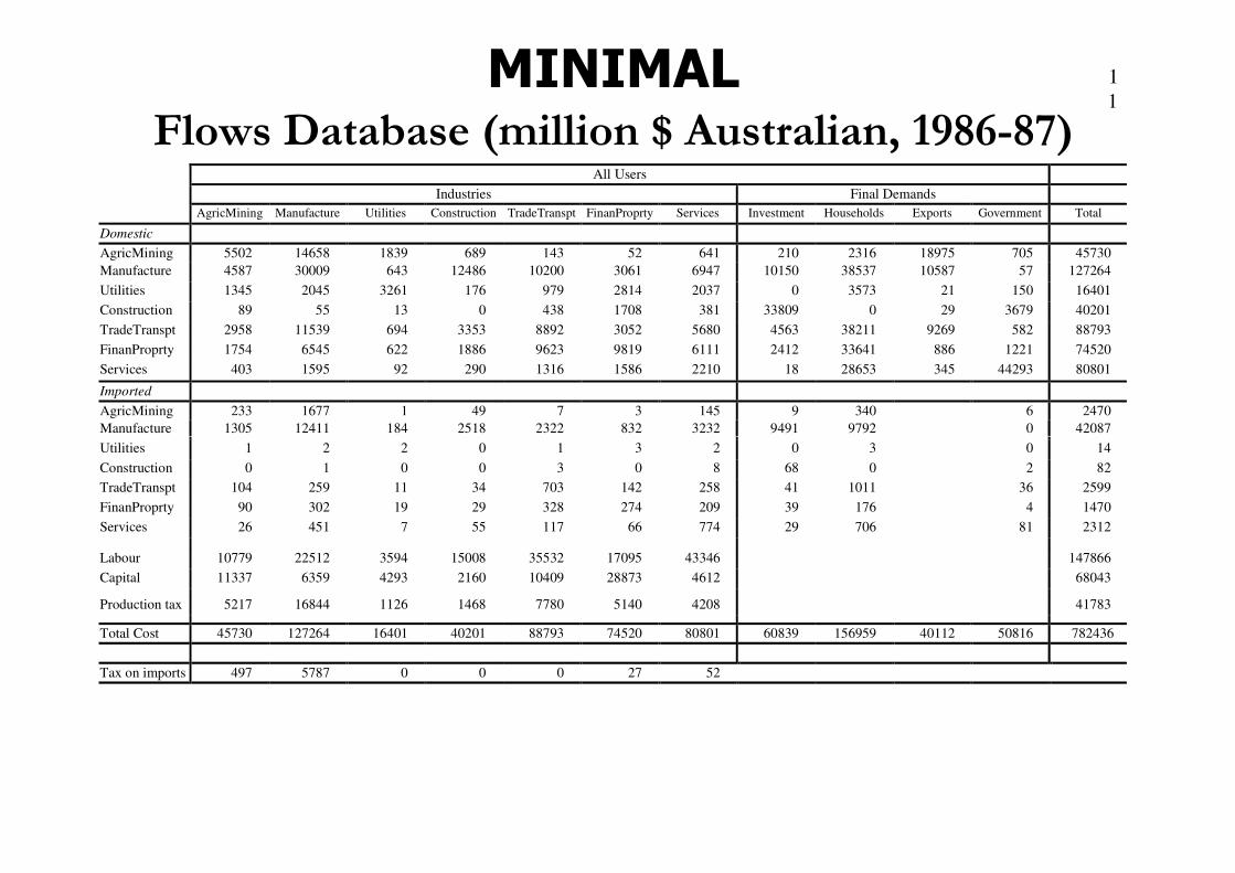
1 MINIMAL - Urząd Miasta Łodzi · MINIMAL Flows Database (million $ Australian, 1986-87) ......
57
1 MINIMAL A Simplified General Equilibrium Model
Transcript of 1 MINIMAL - Urząd Miasta Łodzi · MINIMAL Flows Database (million $ Australian, 1986-87) ......

1
MINIMALA Simplified General Equilibrium Model

Model MINIMAL (1)
Model MINMAL w stosunku do modelu
„wymiany z produkcją” rozszerzony jest o:
• nakłady materiałowe,• nakłady materiałowe,
• handel zagraniczny (eksport i import),
• dodatkowe elementy popytu finalnego
(spożycie rządowe, inwestycje),
• podatki i cła.
Model MINIMAL (2)
• Model MINIMAL, w odróżnieniu od
modelu „wymiany z produkcją”, wyróżnia
tylko jedno reprezentatywne tylko jedno reprezentatywne
gospodarstwo domowe.
• Możliwa interpretacja – wszystkie
gospodarstwa są jednakowe (mają
jednakowe udziały we własności czynników
produkcji). Nie da się badać efektów
redystrybucyjnych.

Model MINIMAL (3)
• Bazą danych modelu jest tablica
przepływów międzygałęziowych
(input-output).(input-output).

Gałęzie/produkty
• W modelu MINIMAL występuje 7 gałęzi
(AgricMining, Manufacture, Utilities,
Construction, TradeTranspt, FinanProprty, Construction, TradeTranspt, FinanProprty,
Services) i tyle samo produktów.
• Zbiór gałęzi: IND; zbiór produktów: COM.
• Każda gałąź wytwarza tylko jeden rodzaj
produktów.
Czynniki produkcji
• Kapitał.
• Praca.
• Materiały (produkty).• Materiały (produkty).
Kapitał i praca to tzw. pierwotne czynniki
produkcji (primary factors).

Elementy popytu
• Popyt finalny:
– popyt inwestycyjny (2),
– konsumpcja gospodarstw domowych (3),
Nr kategorii
popytu w
oznaczeniach
zmiennych
– konsumpcja gospodarstw domowych (3),
– eksport (4)
– konsumpcja rządowa (5)
• Popyt pośredni (zużycie pośrednie) (1)

8
Excerpt 1a: Sets for users
Set ! User categories: IO table columns !
IND # Industries # (AgricMining, Manufacture, Utilities,
Construction, TradeTranspt, FinanProprty, Services);
! subscript i !
FINALUSER # Final demanders # (Investment, Households,
Government, Exports);
USER # All users #= IND union FINALUSER; ! subscript u !
IMPUSER # Non-export demanders: users of imports #IMPUSER # Non-export demanders: users of imports #
(AgricMining, Manufacture, Utilities, Construction,
TradeTranspt, FinanProprty, Services, Investment,
Households, Government);
Subset
IMPUSER is subset of USER;
IND is subset of IMPUSER;

9
Excerpt 1a: Sets for users
FINAL
Investment
Households
AgricMining
Manufacture
IMPUSER
USER
FINAL
USERIND
Households
Government
Exports
Manufacture
Utilities
Construction
TradeTranspt
FinanProprty
Services

1
0
Model DatabaseAbsorption Matrix
1 2 3 4 5
Producers Investors Household Export Government Total Sales
Size ← I → ← 1 → ← 1 → ← 1 → ← 1 →
DomesticFlows
↑C
↓
USE(commodity,"dom",user)
Imported↑C USE(commodity,"imp",user)
memorize
numbers
ImportedFlows
C
↓
USE(commodity,"imp",user)
Labour↑1
↓
FACTOR(labour)
C= Number of Commodities = 7
I = Number of Industries = 7
Capital↑1
↓
FACTOR(capital)
Output tax
↑1
↓
V1PTX
Also V0MTX = Tax on Imports of each commodity
1
1MINIMAL
Flows Database (million $ Australian, 1986-87)All Users
Industries Final Demands
AgricMining Manufacture Utilities Construction TradeTranspt FinanProprty Services Investment Households Exports Government Total
Domestic
AgricMining 5502 14658 1839 689 143 52 641 210 2316 18975 705 45730
Manufacture 4587 30009 643 12486 10200 3061 6947 10150 38537 10587 57 127264
Utilities 1345 2045 3261 176 979 2814 2037 0 3573 21 150 16401
Construction 89 55 13 0 438 1708 381 33809 0 29 3679 40201
TradeTranspt 2958 11539 694 3353 8892 3052 5680 4563 38211 9269 582 88793
FinanProprty 1754 6545 622 1886 9623 9819 6111 2412 33641 886 1221 74520
Services 403 1595 92 290 1316 1586 2210 18 28653 345 44293 80801
Imported
AgricMining 233 1677 1 49 7 3 145 9 340 6 2470
Manufacture 1305 12411 184 2518 2322 832 3232 9491 9792 0 42087
Utilities 1 2 2 0 1 3 2 0 3 0 14
Construction 0 1 0 0 3 0 8 68 0 2 82
TradeTranspt 104 259 11 34 703 142 258 41 1011 36 2599
FinanProprty 90 302 19 29 328 274 209 39 176 4 1470
Services 26 451 7 55 117 66 774 29 706 81 2312
Labour 10779 22512 3594 15008 35532 17095 43346 147866
Capital 11337 6359 4293 2160 10409 28873 4612 68043
Production tax 5217 16844 1126 1468 7780 5140 4208 41783
Total Cost 45730 127264 16401 40201 88793 74520 80801 60839 156959 40112 50816 782436
Tax on imports 497 5787 0 0 0 27 52

1
2
Excerpt 1b: Other sets; Flows DataSet ! Input categories: IO table rows !
COM # Commodities # (AgricMining, Manufacture, Utilities, Construction,
TradeTranspt, FinanProprty, Services); ! subscript c !
SRC # Source of commodities # (dom,imp); ! subscript s !
FAC # Primary factors # (Labour, Capital); ! subscript f !
Coefficient
(all,c,COM)(all,s,SRC)(all,u,USER) USE(c,s,u) # USE matrix #;
(all,f,FAC)(all,i,IND) FACTOR(f,i) # Wages and profits #;(all,f,FAC)(all,i,IND) FACTOR(f,i) # Wages and profits #;
(all,i,IND) V1PTX(i) # Production tax revenue #;
(all,c,COM) V0MTX(c) # import tax revenue #;
File BASEDATA # Flows Data File #;
Read
USE from file BASEDATA header "USE";
FACTOR from file BASEDATA header "1FAC";
V0MTX from file BASEDATA header "0TAR";
V1PTX from file BASEDATA header "1PTX";

1
3
Excerpt 2: Useful aggregates of the dataCoefficient
(all,c,COM)(all,u,USER) USE_S(c,u) # USE matrix, dom+imp
together#;
(all,u,USER) USE_CS(u) # Total user expenditure on goods #;
(all,c,COM)(all,s,SRC) SALES(c,s) # Total value of sales #;
(all,i,IND) V1PRIM(i) # Wages plus profits #;
(all,i,IND) V1TOT(i) # Industry Costs #;
(all,c,COM) V0CIF(c) # Aggregate imports at border prices #;(all,c,COM) V0CIF(c) # Aggregate imports at border prices #;
Formula
(all,c,COM)(all,u,USER) USE_S(c,u) = sum{s,SRC,USE(c,s,u)};
(all,u,USER) USE_CS(u) = sum{c,COM,USE_S(c,u)};
(all,c,COM)(all,s,SRC) SALES(c,s) = sum{u,USER,USE(c,s,u)};
(all,i,IND) V1PRIM(i) = sum{f,FAC,FACTOR(f,i)};
(all,i,IND) V1TOT(i) = V1PRIM(i) + sum{c,COM,USE_S(c,i)};
(all,c,COM) V0CIF(c) = SALES(c,"imp") - V0MTX(c);
1
4
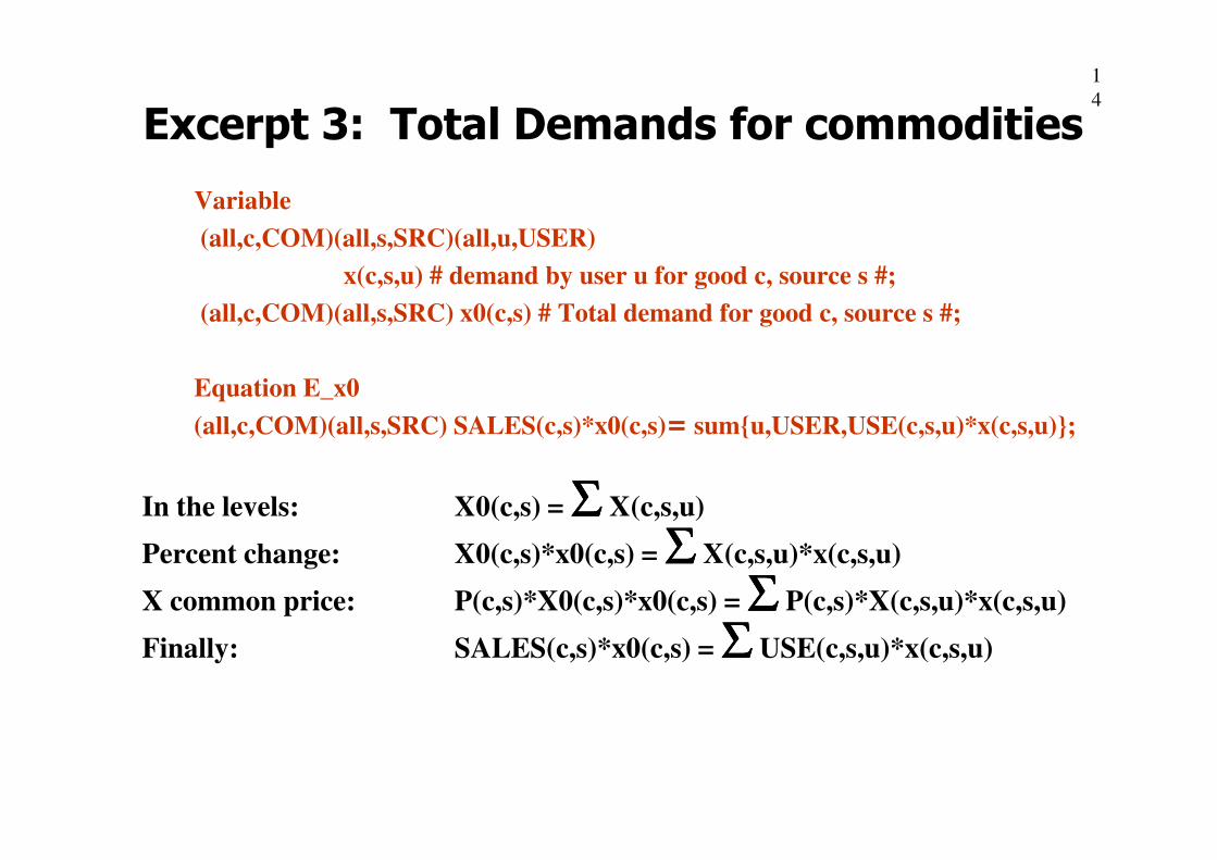
Excerpt 3: Total Demands for commodities
Variable
(all,c,COM)(all,s,SRC)(all,u,USER)
x(c,s,u) # demand by user u for good c, source s #;
(all,c,COM)(all,s,SRC) x0(c,s) # Total demand for good c, source s #;
Equation E_x0
(all,c,COM)(all,s,SRC) SALES(c,s)*x0(c,s)= sum{u,USER,USE(c,s,u)*x(c,s,u)};(all,c,COM)(all,s,SRC) SALES(c,s)*x0(c,s)= sum{u,USER,USE(c,s,u)*x(c,s,u)};
In the levels: X0(c,s) = ΣΣΣΣ X(c,s,u)
Percent change: X0(c,s)*x0(c,s) = ΣΣΣΣ X(c,s,u)*x(c,s,u)
X common price: P(c,s)*X0(c,s)*x0(c,s) = ΣΣΣΣ P(c,s)*X(c,s,u)*x(c,s,u)
Finally: SALES(c,s)*x0(c,s) = ΣΣΣΣ USE(c,s,u)*x(c,s,u)
1
5
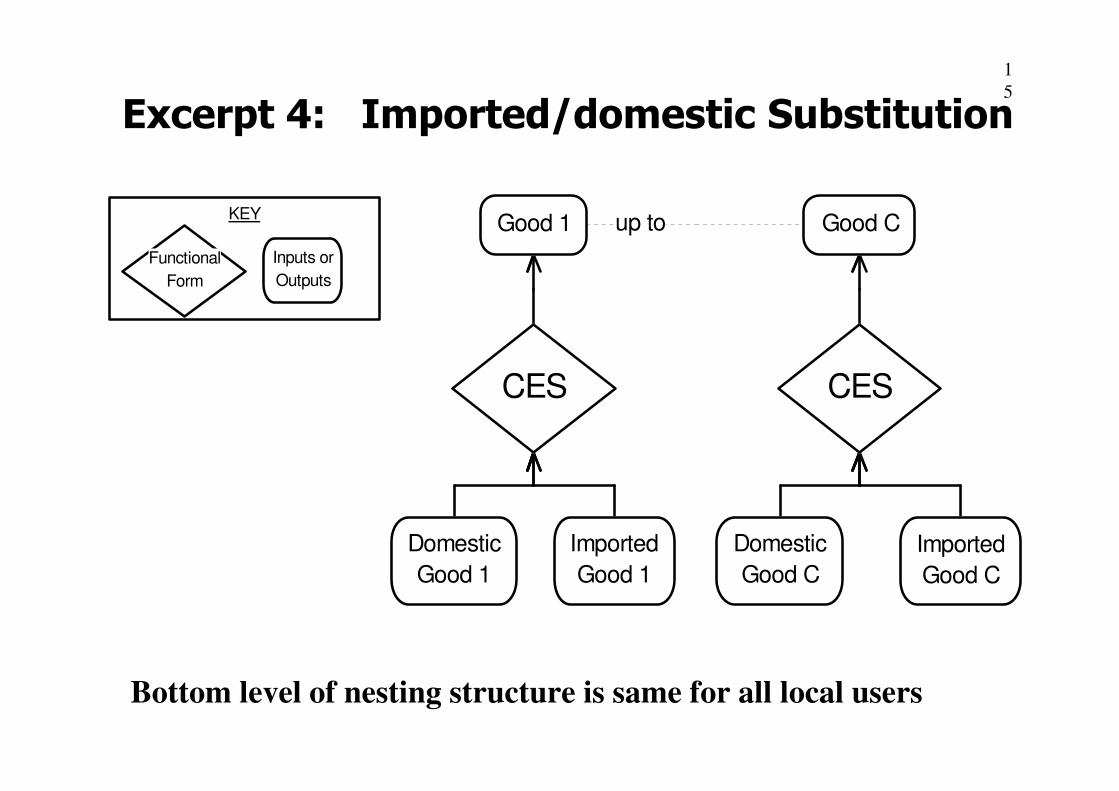
Excerpt 4: Imported/domestic Substitution
KEY
Inputs or
Outputs
Functional
Form
CESCES
up to Good CGood 1
Bottom level of nesting structure is same for all local users
CESCES
Imported
Good C
Domestic
Good C
Imported
Good 1
Domestic
Good 1

Nowe mechanizmy* (1)
Nakłady materiałowe (zużycie pośrednie).
• Zapotrzebowanie na materiały w danej
gałęzi proporcjonalne do jej produkcji.gałęzi proporcjonalne do jej produkcji.
* Nowe w „stosunku do modelu wymiany z produkcją”.

Nowe mechanizmy (2)
Substytucja dóbr krajowych i importowanych.
• Odbiorcy (gospodarstwa domowe, producenci,
inwestorzy, rząd) zgłaszają popyt na „kompozyty”
produktów.produktów.
• Skład kompozytu (tj. udział dóbr krajowych i
importowanych) zmienia się pod wpływem zmian
relacji cen produktów krajowych i
importowanych.
• Możliwości substytucji opisuje funkcja CES.

Nowe mechanizmy (3)
Eksport.
• Popyt zagranicy na dobra krajowe jest funkcją
relacji cen produktów krajowych do światowych
cen tych samych produktów.cen tych samych produktów.
• Siłę wpływu relatywnych cen na eksport wyrażona
jest za pomocą (stałej) elastyczności.
• Eksport może zmieniać się też niezależnie od cen,
np. pod wpływem zmian koniunktury na świecie
(zmienne f4q).

1
9
Variable
(all,c,COM)(all,s,SRC) p(c,s) # user price of good c, source s #;
(all,c,COM)(all,u,IMPUSER) p_s(c,u) # user price of composite good c #;
(all,c,COM)(all,u,IMPUSER) x_s(c,u) # use of composite good c #;
Coefficient
(all,c,COM) SIGMA(c) # elasticity of substitution: domestic/imported #;
(all,c,COM)(all,s,SRC)(all,u,IMPUSER) SRCSHR(c,s,u) # imp/dom shares #;
Read SIGMA from file BASEDATA header "ARM";
Formula (all,c,COM)(all,s,SRC)(all,u,IMPUSER)
Excerpt 4: CES Imported/domestic Substitution
Formula (all,c,COM)(all,s,SRC)(all,u,IMPUSER)
SRCSHR(c,s,u) = USE(c,s,u)/USE_S(c,u);
Equation E_x
(all,c,COM)(all,s,SRC)(all,u,IMPUSER)
x(c,s,u) = x_s(c,u) - SIGMA(c)*[p(c,s) - p_s(c,u)];
Equation E_p_s
(all,c,COM)(all,u,IMPUSER) p_s(c,u) = sum{s,SRC, SRCSHR(c,s,u)*p(c,s)};
xs = xaverage - σσσσ[ps - paverage]
paverage = ΣΣΣΣSs.ps
•
2
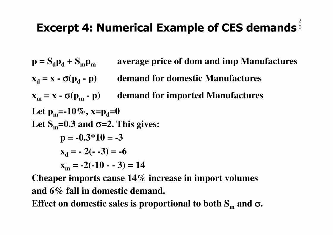
0Excerpt 4: Numerical Example of CES demands
p = Sdpd + Smpm average price of dom and imp Manufactures
xd = x - σσσσ(pd - p) demand for domestic Manufactures
xm = x - σσσσ(pm - p) demand for imported Manufactures
Let pm=-10%, x=pd=0
σσ
•
m d
Let Sm=0.3 and σσσσ=2. This gives:
p = -0.3*10 = -3
xd = - 2(- -3) = -6
xm = -2(-10 - - 3) = 14
Cheaper imports cause 14% increase in import volumes
and 6% fall in domestic demand.
Effect on domestic sales is proportional to both Sm and σσσσ.

2
1KEY
Inputs or
Outputs
Functional
Form
Leontief
up to Primary
Factors
Good CGood 1
Output
Nested Structure of Production
CESCESCES
CapitalLabour
Factors
Imported
Good C
Domestic
Good C
Imported
Good 1
Domestic
Good 1

2
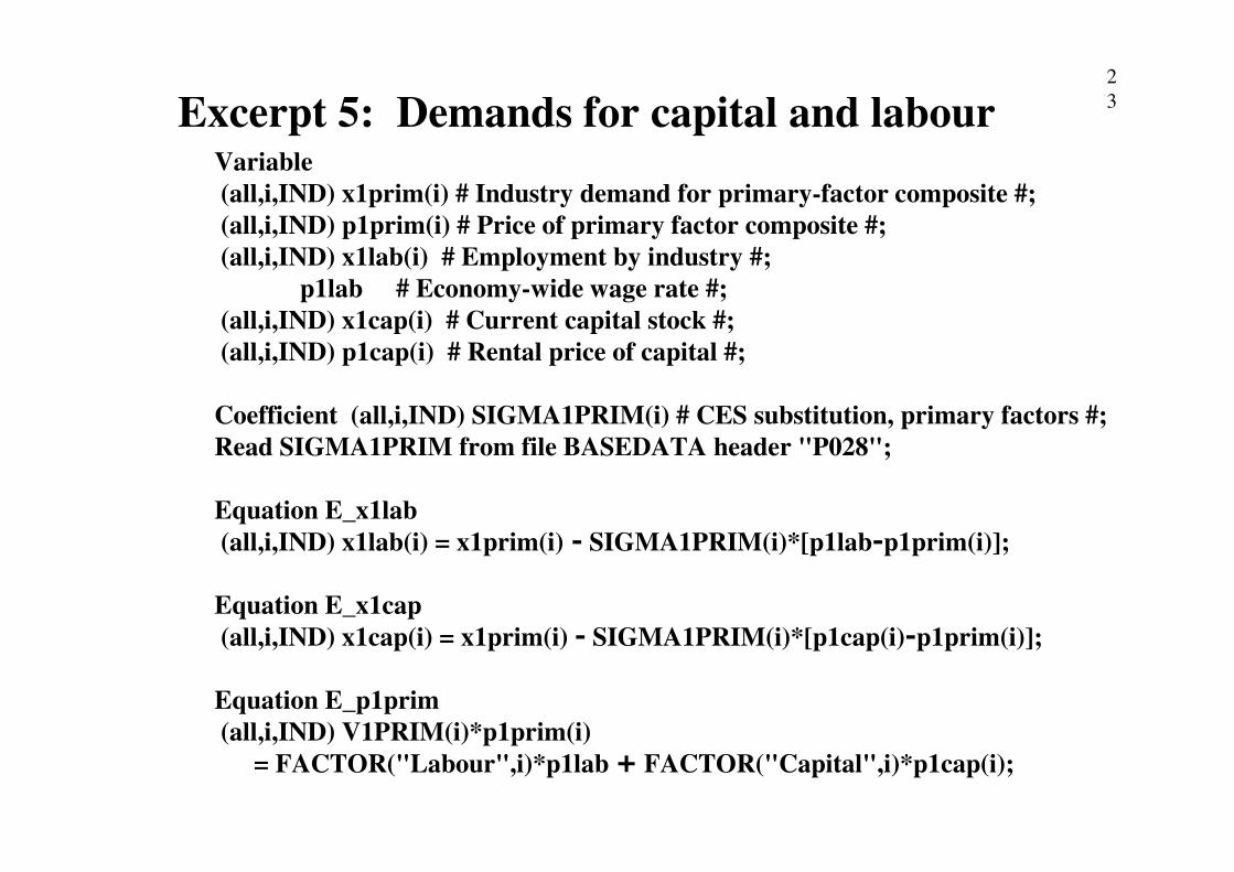
2Demands for primary factors
Choose inputs of labour and capital, X1LAB(i) and X1CAP(i),
to minimize primary factor cost, P1LAB*X1LAB(i) + P1CAP(i)*X1CAP(i)
where X1PRIM(i) = CES[ X1LAB(i), X1CAP(i) ],
regarding as fixed: P1LAB and P1CAP(i) and X1PRIM(i).
Answer: (all,i,IND)
x1lab(i) = x1prim(i) - SIGMA1PRIM(i)*[p1lab-p1prim(i)];x1lab(i) = x1prim(i) - SIGMA1PRIM(i)*[p1lab-p1prim(i)];
x1cap(i) = x1prim(i) - SIGMA1PRIM(i)*[p1cap(i)-p1prim(i)];
V1PRIM(i)*p1prim(i) =FACTOR("Labour",i)*p1lab + FACTOR("Capital",i)*p1cap(i);
Could write
p1prim(i) = S1LAB(i)*p1lab + S1CAP(i)*p1cap(i),
x1prim(i) = S1LAB(i)*x1lab(i) + S1CAP(i)*x1cap(i)
S1LAB and S1CAP are shares of labour and capital in primary factor cost.
2
3Excerpt 5: Demands for capital and labourVariable
(all,i,IND) x1prim(i) # Industry demand for primary-factor composite #;
(all,i,IND) p1prim(i) # Price of primary factor composite #;
(all,i,IND) x1lab(i) # Employment by industry #;
p1lab # Economy-wide wage rate #;
(all,i,IND) x1cap(i) # Current capital stock #;
(all,i,IND) p1cap(i) # Rental price of capital #;
Coefficient (all,i,IND) SIGMA1PRIM(i) # CES substitution, primary factors #;
Read SIGMA1PRIM from file BASEDATA header "P028";Read SIGMA1PRIM from file BASEDATA header "P028";
Equation E_x1lab
(all,i,IND) x1lab(i) = x1prim(i) - SIGMA1PRIM(i)*[p1lab-p1prim(i)];
Equation E_x1cap
(all,i,IND) x1cap(i) = x1prim(i) - SIGMA1PRIM(i)*[p1cap(i)-p1prim(i)];
Equation E_p1prim
(all,i,IND) V1PRIM(i)*p1prim(i)
= FACTOR("Labour",i)*p1lab + FACTOR("Capital",i)*p1cap(i);
2
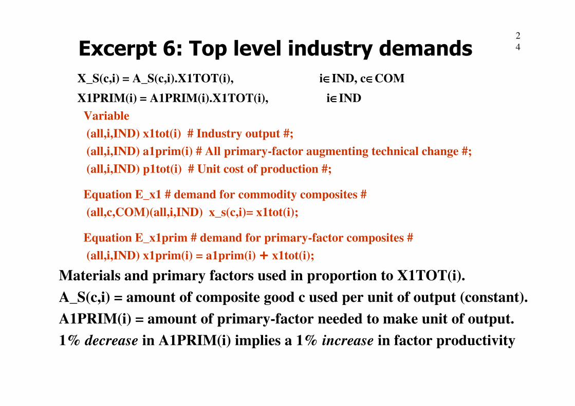
4Excerpt 6: Top level industry demands
X_S(c,i) = A_S(c,i).X1TOT(i), i∈∈∈∈IND, c∈∈∈∈COM
X1PRIM(i) = A1PRIM(i).X1TOT(i), i∈∈∈∈IND
Variable
(all,i,IND) x1tot(i) # Industry output #;
(all,i,IND) a1prim(i) # All primary-factor augmenting technical change #;
(all,i,IND) p1tot(i) # Unit cost of production #;
Equation E_x1 # demand for commodity composites #
(all,c,COM)(all,i,IND) x_s(c,i)= x1tot(i);
Equation E_x1prim # demand for primary-factor composites #
(all,i,IND) x1prim(i) = a1prim(i) + x1tot(i);
Materials and primary factors used in proportion to X1TOT(i).
A_S(c,i) = amount of composite good c used per unit of output (constant).
A1PRIM(i) = amount of primary-factor needed to make unit of output.
1% decrease in A1PRIM(i) implies a 1% increase in factor productivity
2
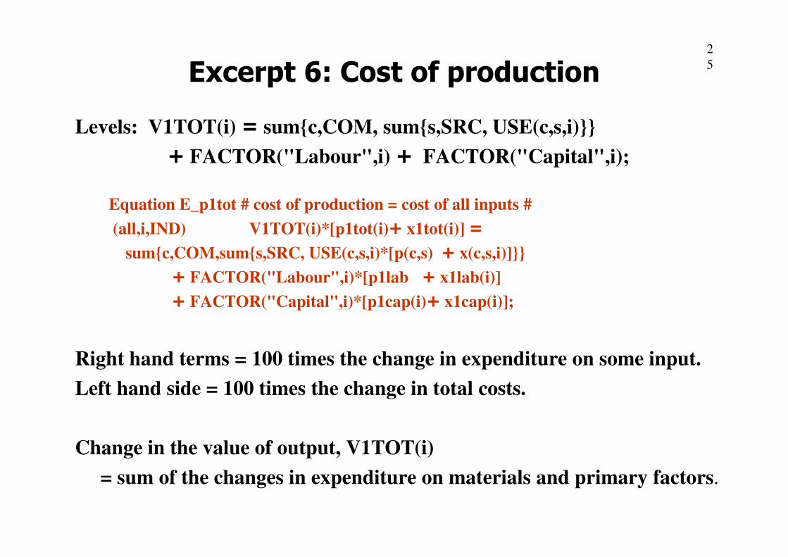
5Excerpt 6: Cost of production
Levels: V1TOT(i) = sum{c,COM, sum{s,SRC, USE(c,s,i)}}
+ FACTOR("Labour",i) + FACTOR("Capital",i);
Equation E_p1tot # cost of production = cost of all inputs #
(all,i,IND) V1TOT(i)*[p1tot(i)+ x1tot(i)] =
sum{c,COM,sum{s,SRC, USE(c,s,i)*[p(c,s) + x(c,s,i)]}}
+ FACTOR("Labour",i)*[p1lab + x1lab(i)]+ FACTOR("Labour",i)*[p1lab + x1lab(i)]
+ FACTOR("Capital",i)*[p1cap(i)+ x1cap(i)];
Right hand terms = 100 times the change in expenditure on some input.
Left hand side = 100 times the change in total costs.
Change in the value of output, V1TOT(i)
= sum of the changes in expenditure on materials and primary factors.
2
6
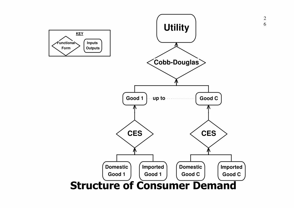
KEY
Inputs
Outputs
Functional
Form
Cobb-Douglas
up to Good CGood 1
Utility
Structure of Consumer Demand
CESCES
Imported
Good C
Domestic
Good C
Imported
Good 1
Domestic
Good 1
2
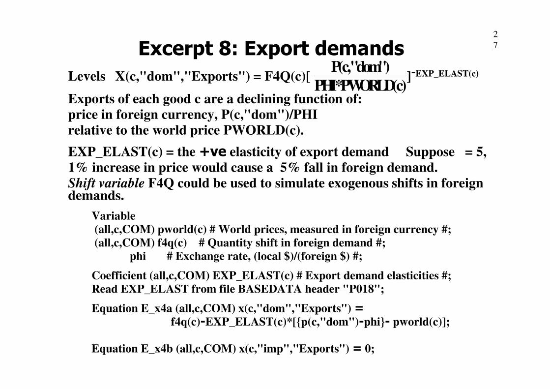
7Excerpt 8: Export demands
Levels X(c,"dom","Exports") = F4Q(c)[ ]-EXP_ELAST(c)
Exports of each good c are a declining function of:price in foreign currency, P(c,"dom")/PHIrelative to the world price PWORLD(c).
EXP_ELAST(c) = the +ve elasticity of export demand Suppose = 5,1% increase in price would cause a 5% fall in foreign demand.Shift variable F4Q could be used to simulate exogenous shifts in foreign demands.
P(c,"dom")PHI*PWORLD(c)
demands.
Variable(all,c,COM) pworld(c) # World prices, measured in foreign currency #;(all,c,COM) f4q(c) # Quantity shift in foreign demand #;
phi # Exchange rate, (local $)/(foreign $) #;
Coefficient (all,c,COM) EXP_ELAST(c) # Export demand elasticities #;Read EXP_ELAST from file BASEDATA header "P018";
Equation E_x4a (all,c,COM) x(c,"dom","Exports") =f4q(c)-EXP_ELAST(c)*[{p(c,"dom")-phi}- pworld(c)];
Equation E_x4b (all,c,COM) x(c,"imp","Exports") = 0;

2
8Excerpt 9: Domestic market clearing and prices
Subset COM is subset of IND;
Equation E_x1tot (all,c,COM) x1tot(c) = x0(c,"dom");
Variable (change)
(all,c,COM) Delptxrate(c) # Ordinary change in rate of domestic tax #;
Equation E_pA (all,c,COM)
p(c,"dom") = p1tot(c) +100*[V1TOT(c)/(V1TOT(c)+V1PTX(c))]*Delptxrate(c);
E_x1tot says: Output of each industry, X1TOT(i) =total demand for the domestically produced commodity,
X0(c,"dom").
User price = production cost + taxP(c,"dom") = P1TOT(c)*[1 + PTXRATE(c)]
Rule: %Change A = 100.∆∆∆∆A/A
So: %Change [1+A] = 100.∆∆∆∆A/[1+A]1/[1 + PTXRATE(c)] = share of production cost in user price
= V1TOT(c)/[V1TOT(c)+V1PTX(c)]

2
9Excerpt 10: Prices of imports
Levels: P(c,"imp") = PHI*PWORLD(c)*[1 + MTXRATE(c)]
Variable
(change)(all,c,COM) Delmtxrate(c)
# Ordinary change in rate of import tax #;
Equation E_pBEquation E_pB
(all,c,COM)
p(c,"imp") = pworld(c) + phi +100*[V0CIF(c)/SALES(c,"imp")]*Delmtxrate(c);
share of border cost in
user price
3
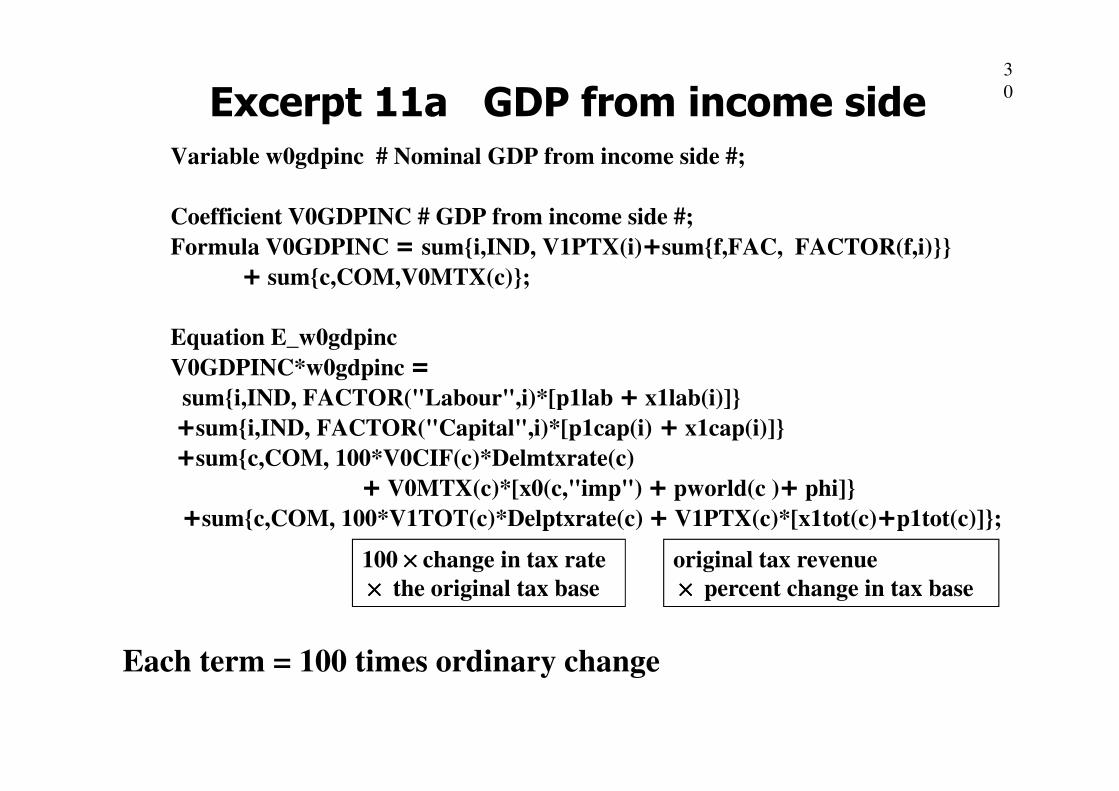
0Excerpt 11a GDP from income sideVariable w0gdpinc # Nominal GDP from income side #;
Coefficient V0GDPINC # GDP from income side #;
Formula V0GDPINC = sum{i,IND, V1PTX(i)+sum{f,FAC, FACTOR(f,i)}}
+ sum{c,COM,V0MTX(c)};
Equation E_w0gdpinc
V0GDPINC*w0gdpinc =
sum{i,IND, FACTOR("Labour",i)*[p1lab + x1lab(i)]}sum{i,IND, FACTOR("Labour",i)*[p1lab + x1lab(i)]}
+sum{i,IND, FACTOR("Capital",i)*[p1cap(i) + x1cap(i)]}
+sum{c,COM, 100*V0CIF(c)*Delmtxrate(c)
+ V0MTX(c)*[x0(c,"imp") + pworld(c )+ phi]}
+sum{c,COM, 100*V1TOT(c)*Delptxrate(c) + V1PTX(c)*[x1tot(c)+p1tot(c)]};
Each term = 100 times ordinary change
100 ×××× change in tax rate
×××× the original tax base
original tax revenue
×××× percent change in tax base

3
1
Excerpt 11b GDP from expenditure sideGDP = C+I+G+X-M
Variable
w0gdpexp # Nominal GDP from expenditure side #;
p0gdpexp # GDP price index, expenditure side #;
x0gdpexp # Real GDP from expenditure side #;
Coefficient
V0GDPEXP # GDP from expenditure side #;
Formula
V0GDPEXP = sum{c,COM, sum{s,SRC,sum{u,FINALUSER, USE(c,s,u)}}-
V0GDPEXP = sum{c,COM, sum{s,SRC,sum{u,FINALUSER, USE(c,s,u)}}- V0CIF(c)};
Equation E_w0gdpexp
V0GDPEXP*w0gdpexp =sum{c,COM, sum{s,SRC,sum{u,FINALUSER,
USE(c,s,u)*[p(c,s)+x(c,s,u)]}}
- V0CIF(c)*[x0(c,"imp")+ pworld(c)+phi]};
Equation E_p0gdpexp
V0GDPEXP*p0gdpexp = sum{c,COM,
sum{s,SRC,sum{u,FINALUSER, USE(c,s,u)*p(c,s)}} -V0CIF(c)*[pworld(c)+phi]};
Equation E_x0gdpexp x0gdpexp = w0gdpexp - p0gdpexp

3
2Excerpt 13a More macro variablesVariablex4tot # Export volume index #;p4tot # Export price index #;p2tot # Investment price index #;x0cif_c # Import volume index, CIF prices #;
Equation E_x4totsum{c,COM, USE(c,"dom","Exports")*[x4tot - x(c,"dom","Exports")]} = 0;
Equation E_p4totsum{c,COM, USE(c,"dom","Exports")*[p4tot - p(c,"dom")]} = 0;
Equation E_p2totEquation E_p2totsum{c,COM, sum{s,SRC, USE(c,s,"Investment")*[p2tot - p(c,s)]}} = 0;
Equation E_x0cif_csum{c,COM, V0CIF(c)*[x0cif_c - x0(c,"imp")]}=0;
Equation E_x4tot might have been written:
sum{c,COM,USE(c,"dom","Exports")}*x4tot =
sum{c,COM,USE(c,"dom","Exports")*x(c,"dom","Exports")};

3
3
Excerpt 13b Balance of Trade/GDP
Variable (change) delB # (Balance of trade)/GDP #;
Equation E_delB 100*V0GDPEXP*delB=
sum{c,COM, USE(c,"dom","Exports")*
[p(c,"dom")+x(c,"dom","Exports") - w0gdpexp]
- V0CIF(c)*[x0(c,"imp")+ pworld(c)+phi - w0gdpexp]};
B = [X-M]/GDP
B*GDP = [X-M]B*GDP = [X-M]
GDP*∆∆∆∆B + B*∆∆∆∆GDP = ∆∆∆∆[X-M]
100*GDP*∆∆∆∆B + 100*B*∆∆∆∆GDP = 100*∆∆∆∆[X-M]
100*GDP*∆∆∆∆B + B*GDP*gdp = Xx -Mm
100*GDP*∆∆∆∆B + [X-M]*gdp = Xx - Mm
100*GDP*∆∆∆∆B = X[x-gdp] - M[m-gdp]
3
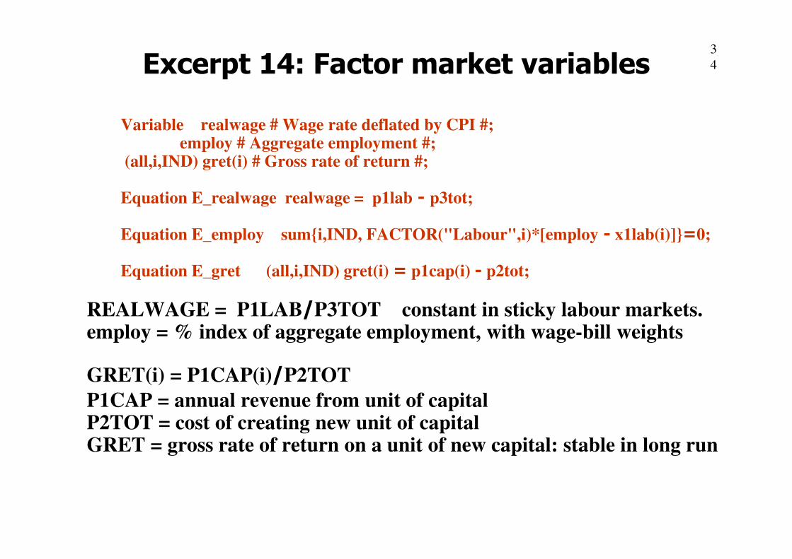
4Excerpt 14: Factor market variables
Variable realwage # Wage rate deflated by CPI #;employ # Aggregate employment #;
(all,i,IND) gret(i) # Gross rate of return #;
Equation E_realwage realwage = p1lab - p3tot;
Equation E_employ sum{i,IND, FACTOR("Labour",i)*[employ - x1lab(i)]}=0;
Equation E_gret (all,i,IND) gret(i) = p1cap(i) - p2tot;Equation E_gret (all,i,IND) gret(i) = p1cap(i) - p2tot;
REALWAGE = P1LAB/P3TOT constant in sticky labour markets.employ = % index of aggregate employment, with wage-bill weights
GRET(i) = P1CAP(i)/P2TOT
P1CAP = annual revenue from unit of capitalP2TOT = cost of creating new unit of capitalGRET = gross rate of return on a unit of new capital: stable in long run

3
5Excerpt 15: Updating the flows data
Updates tell GEMPACK how to make post-simulation or updated database.
Product updates:
Formula: USE(c,s,u) = P(c,s)*X(c,s,u) c∈∈∈∈COM, s∈∈∈∈SRC, u∈∈∈∈USER
Update: USE(c,s,u) →→→→ USE(c,s,u)*[1+0.01*p(c,s)+0.01*x(c,s,u)]
Update
(all,c,COM)(all,s,SRC)(all,u,USER) USE(c,s,u) = p(c,s)*x(c,s,u);
(all,i,IND) FACTOR("Labour",i) = p1lab*x1lab(i);
(all,i,IND) FACTOR("Capital",i) = p1cap(i)*x1cap(i);(all,i,IND) FACTOR("Capital",i) = p1cap(i)*x1cap(i);
Change updates: explicit formulae for ordinary change
(change)(all,c,COM) V0MTX(c) =
V0CIF(c)*Delmtxrate(c) + 0.01*V0MTX(c)*[x0(c,"imp")+ pworld(c)+phi];
(change)(all,c,COM) V1PTX(c) =
V1TOT(c)*Delptxrate(c) + 0.01*V1PTX(c)*[x1tot(c)+ p1tot(c)];
change in tax rate
×××× the original tax base
original tax revenue
×××× proportional change (=%/100) in tax base
3
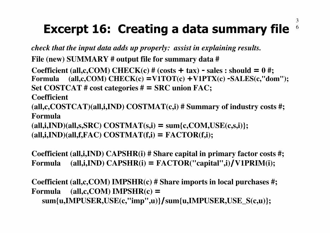
6Excerpt 16: Creating a data summary file
check that the input data adds up properly: assist in explaining results.
File (new) SUMMARY # output file for summary data #
Coefficient (all,c,COM) CHECK(c) # (costs + tax) - sales : should = 0 #;Formula (all,c,COM) CHECK(c) =V1TOT(c) +V1PTX(c) -SALES(c,"dom");
Set COSTCAT # cost categories # = SRC union FAC;Coefficient
(all,c,COSTCAT)(all,i,IND) COSTMAT(c,i) # Summary of industry costs #;
FormulaFormula
(all,i,IND)(all,s,SRC) COSTMAT(s,i) = sum{c,COM,USE(c,s,i)};
(all,i,IND)(all,f,FAC) COSTMAT(f,i) = FACTOR(f,i);
Coefficient (all,i,IND) CAPSHR(i) # Share capital in primary factor costs #;
Formula (all,i,IND) CAPSHR(i) = FACTOR("capital",i)/V1PRIM(i);
Coefficient (all,c,COM) IMPSHR(c) # Share imports in local purchases #;
Formula (all,c,COM) IMPSHR(c) = sum{u,IMPUSER,USE(c,"imp",u)}/sum{u,IMPUSER,USE_S(c,u)};

3
7Closing the model
Each equation explains a variable.
More variables than equations.
Endogenous variables: explained by model
Exogenous variables: set by user
Closure: choice of exogenous variables
Many possible closures
Number of endogenous variables = Number of equations
One way to construct a closure:
(a) Find the variable that each equation explains; it is endogenous.
(b) Other variables, not explained by equations, are exogenous.
MINIMAL equations are named after the variable they SEEM to explain.
3
8
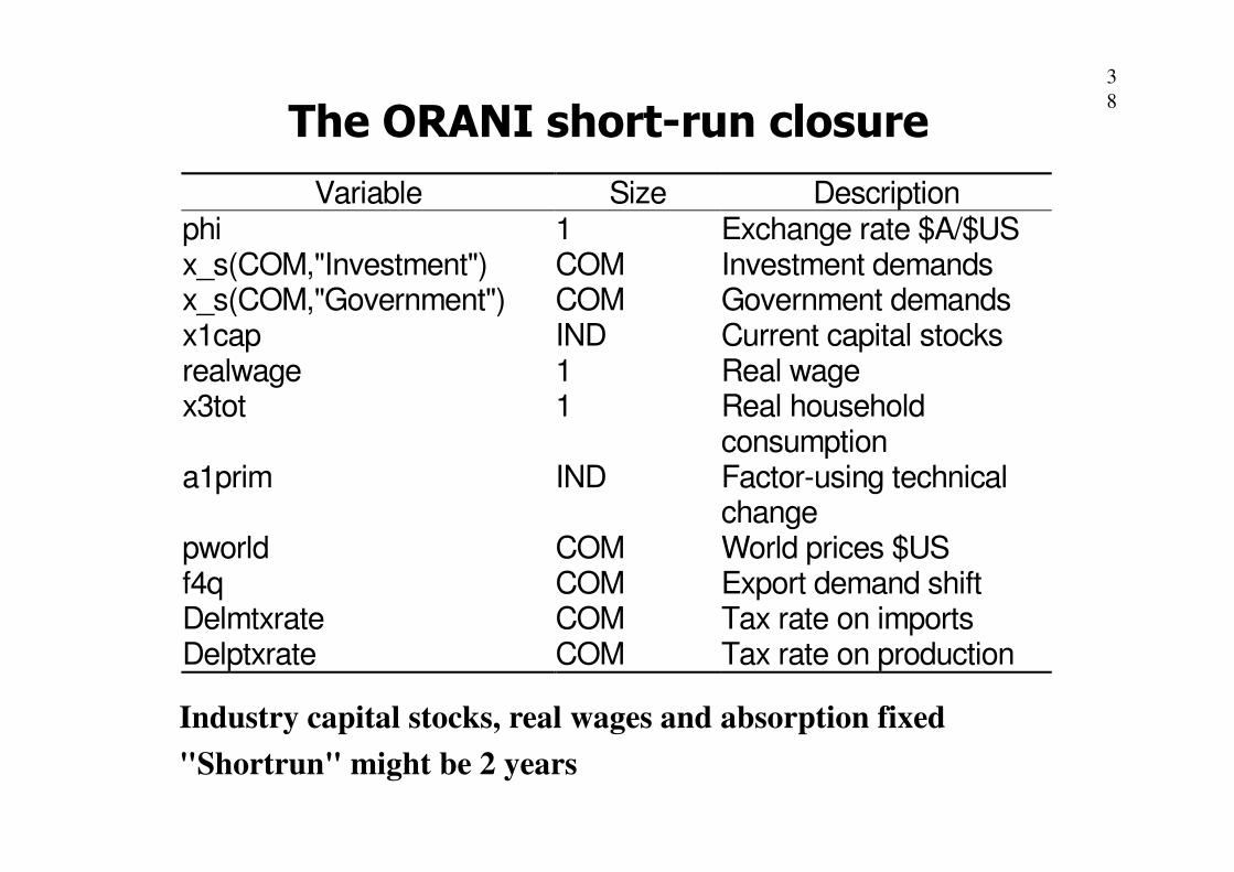
The ORANI short-run closure
Variable Size Descriptionphi 1 Exchange rate $A/$USx_s(COM,"Investment") COM Investment demandsx_s(COM,"Government") COM Government demandsx1cap IND Current capital stocksrealwage 1 Real wagex3tot 1 Real household
consumptionconsumptiona1prim IND Factor-using technical
changepworld COM World prices $USf4q COM Export demand shiftDelmtxrate COM Tax rate on importsDelptxrate COM Tax rate on production
Industry capital stocks, real wages and absorption fixed
"Shortrun" might be 2 years
3
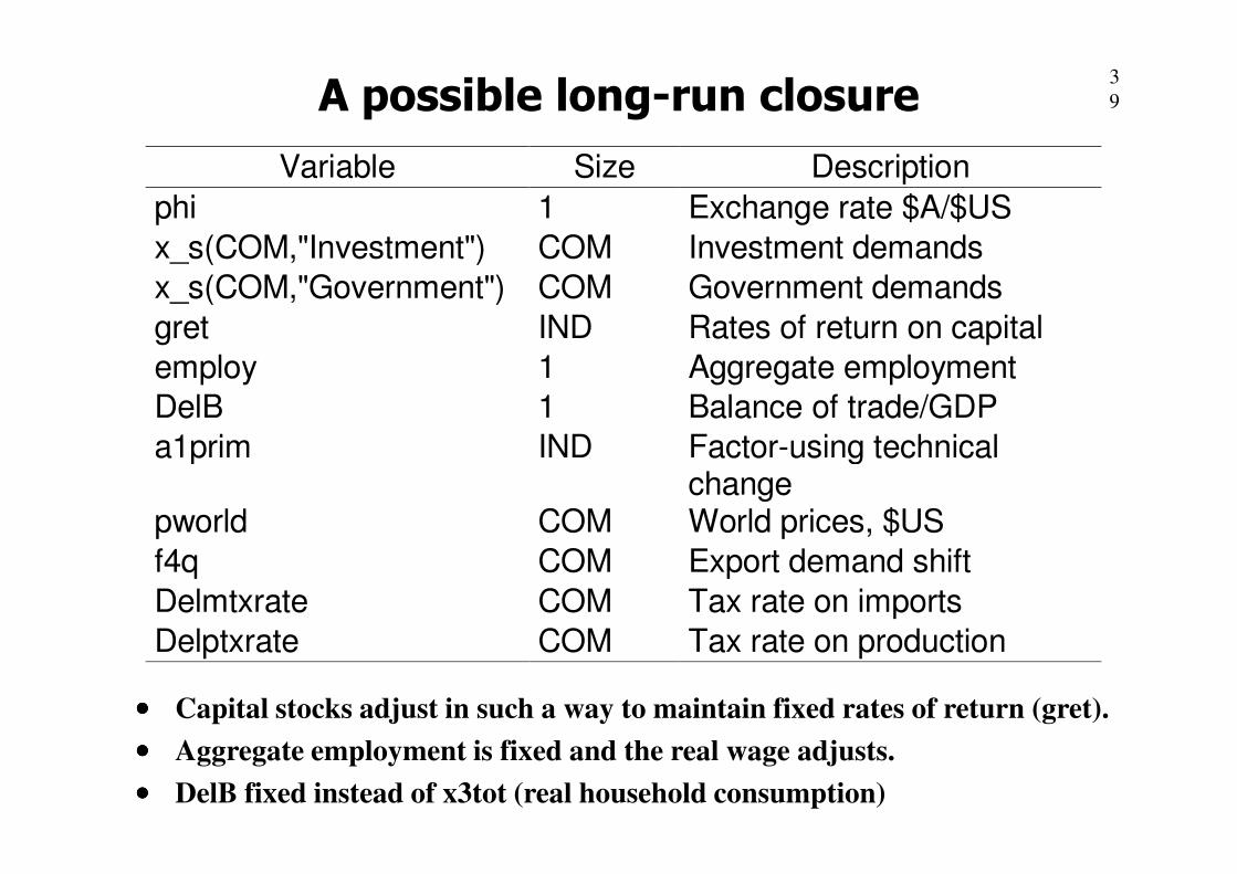
9A possible long-run closure
Variable Size Description
phi 1 Exchange rate $A/$US
x_s(COM,"Investment") COM Investment demands
x_s(COM,"Government") COM Government demands
gret IND Rates of return on capital
employ 1 Aggregate employmentDelB 1 Balance of trade/GDP
a1prim IND Factor-using technicala1prim IND Factor-using technicalchange
pworld COM World prices, $US
f4q COM Export demand shift
Delmtxrate COM Tax rate on imports
Delptxrate COM Tax rate on production
•••• Capital stocks adjust in such a way to maintain fixed rates of return (gret).
•••• Aggregate employment is fixed and the real wage adjusts.
•••• DelB fixed instead of x3tot (real household consumption)

4
0Different closures
Many closures might be used for different purposes.
No unique natural or correct closure.
Must be at least one exogenous variable measured in local
currency units.
Normally just one — called the numeraire.Normally just one — called the numeraire.
Often the exchange rate, phi, or p3tot, the CPI.
Some quantity variables must be exogenous, such as:
•••• primary factor endowments
•••• final demand aggregates

4
1Three Macro Agnostics

4
2Three Macro Don't Knows
•••• ΑΑΑΑbsolute price level. Numeraire choice determines
whether changes in the real exchange rate appear as
changes in domestic prices or in changes in the exchange
rate. Real variables unaffected.
•••• Labour supply. Closure determines whether labour •••• Labour supply. Closure determines whether labour
market changes appear as changes in either wage or
employment.
•••• Size and composition of absorption. Either exogenous or
else adjusting to accommodate fixed trade balance.
Closure determines how changes in national income
appear.
4
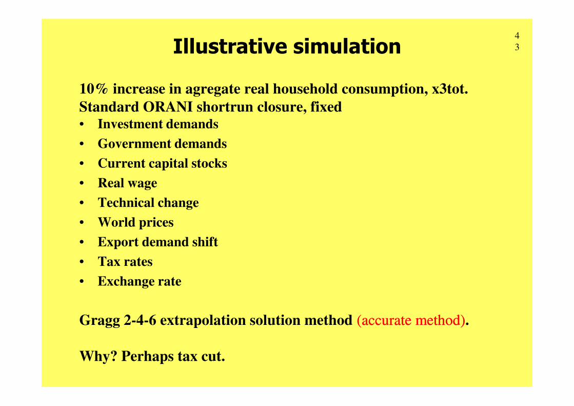
3Illustrative simulation
10% increase in agregate real household consumption, x3tot.
Standard ORANI shortrun closure, fixed• Investment demands
• Government demands
• Current capital stocks
• Real wage
• Technical change• Technical change
• World prices
• Export demand shift
• Tax rates
• Exchange rate
Gragg 2-4-6 extrapolation solution method (accurate method)(accurate method).
Why? Perhaps tax cut.

4
4Illustrative simulation
Results: GDP up, price level up, real appreciation.
Consumption is 60% of GDP, but GDP up only 1%
Leakage: exports down, imports up
Increased output prices cause exports to fall.Increased output prices cause exports to fall.
and imports expand at the expense of domestic sales.

4
5Table1 : Consumption increase: macro results
Variable Description % changeemploy Aggregate employment 111...222444p1lab Economy-wide wage rate 7.69p3tot Consumer price index 7.69phi Exchange rate, (local $)/(foreign $) 0.00realwage Wage rate deflated by CPI 0.00w3tot Nominal total household consumption 18.46x3tot Real household consumption 10.00x3tot Real household consumption 10.00w0gdpexp Nominal GDP from income side 9.23w0gdpinc Nominal GDP from expenditure side 9.23p0gdpexp GDP price index, expenditure side 8.20x0gdpexp Real GDP from expenditure side 000...999555x4tot Export volume index ---111999...777111p4tot Export price index 4.49p2tot Investment price index 5.71x0cif_c Import volume index, CIF prices 111222...555111delB Ordinary change, (Balance of trade)/GDP ---000...000444

4
6Causation in Short-run Closure
Real Wage
Capital StocksTech Change
Rate of
return on
capital
EndogenousExogenous
Private
ConsumptionInvestment
Government
Consumption
Capital StocksTech Change
Trade
balance
Employment
GDP = +++

4
7
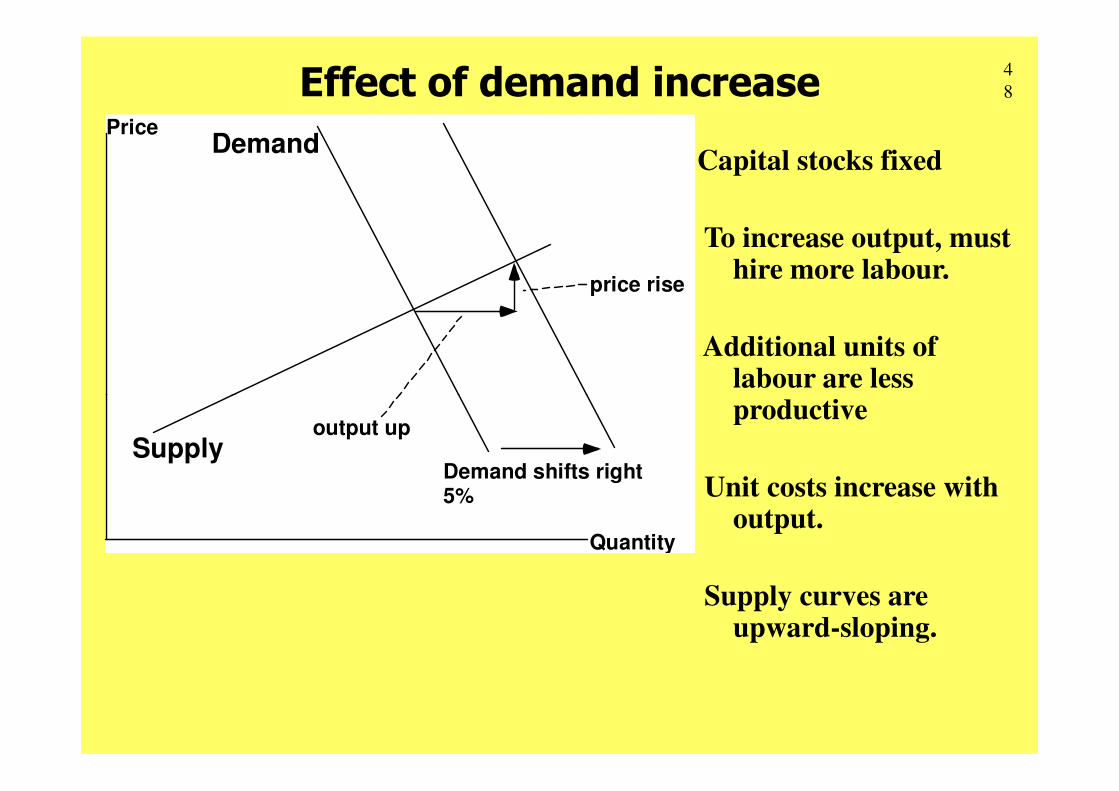
Why higher prices?ShortShort--run: industry capital stocks fixedrun: industry capital stocks fixedTo increase output, must hire more labour.
Additional units of labour are less productive
Unit costs increase with output.
Supply curve are upward-sloping.
The more capital-intensive the sector, the steeper is supply curveThe more capital-intensive the sector, the steeper is supply curve
Largest price rise is for FinanProprty.
Circle of price risesCircle of price risesIncreases in output price in one industry raises input costs in others
Higher consumer prices increase the nominal wage because real wage rate is fixed.
All domestic prices rise.
4
8Effect of demand increasePrice
Demand
price rise
Capital stocks fixed
To increase output, must hire more labour.
Additional units of labour are less productive
Quantity
Demand shifts right5%
output upSupply
productive
Unit costs increase with output.
Supply curves are upward-sloping.
4
9
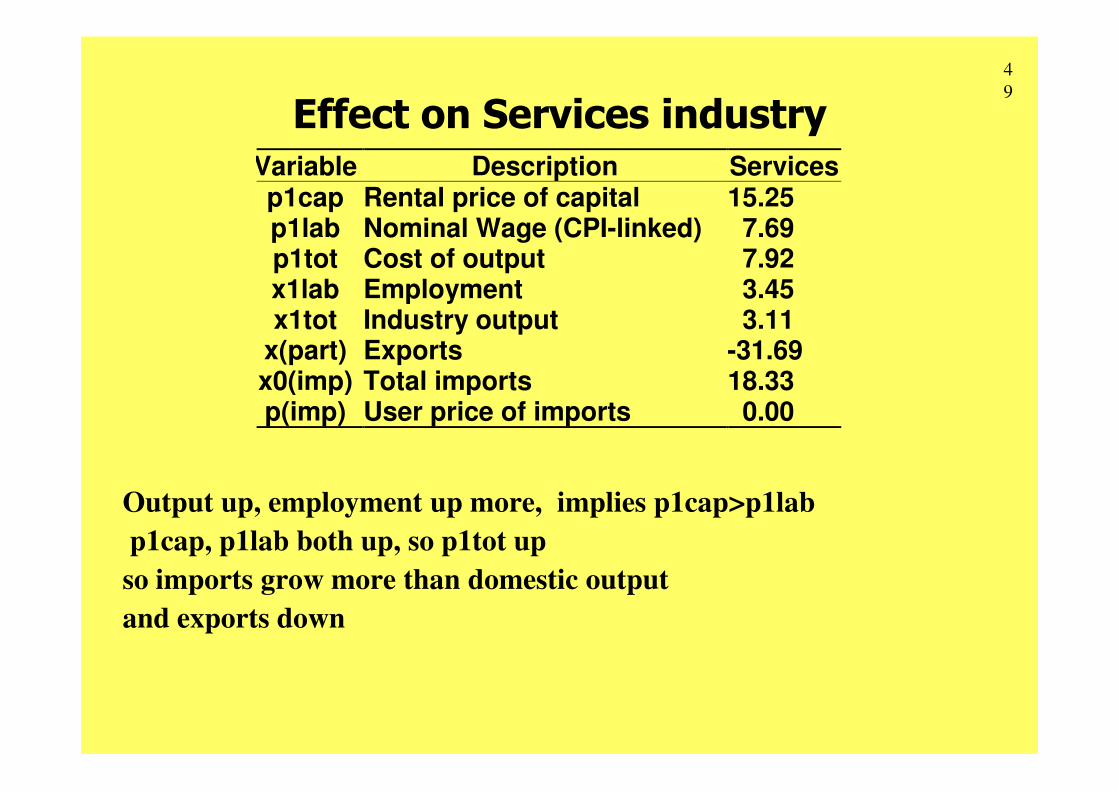
Variable Description Servicesp1cap Rental price of capital 15.25p1lab Nominal Wage (CPI-linked) 7.69p1tot Cost of output 7.92x1lab Employment 3.45x1tot Industry output 3.11
x(part) Exports -31.69x0(imp) Total imports 18.33
Effect on Services industry
p(imp) User price of imports 0.00
Output up, employment up more, implies p1cap>p1lab
p1cap, p1lab both up, so p1tot up
so imports grow more than domestic output
and exports down

5
0Effects of increased input costs
Non-traded sectors: inelastic demand,
pass on higher costs without losing sales.Price
InelasticDemand Supply curve
shifts up
large price rise
Price
ElasticDemand
Supply curveshifts up
small price rise
Export-oriented industries, such as AgricMining, are not able to do so. Import-competers, such as Manufacture, are also vulnerable.
Not shown: right shifts in demand for consumer goods:
Manufacture, TradeTranspt, FinanProprty, and Services
Quantity
small outputfall
large price rise
Quantity
large output fall

5
1GDP IdentityRealGDP = F(Capital,Labour) approximate aggregate relation
GDP from income side:• gdp = Skk + Sll k=0• gdp = Sll
• 0.95 = (approx) (0.68)*1.24 = 0.84
GDP from expenditure side: • RealGDP = C + I + G + (X-M)• RealGDP = C + I + G + (X-M)• I, G fixed, C exogenously increased (by 6% of GDP).• (X-M) changes to make income GDP = expenditure GDP
Why is the change in GDP 1 percent and not 6 percent? GDP = C + I + G + (X-M); Exogenous %∆∆∆∆C= 10; %∆∆∆∆I, %∆∆∆∆G = 0.
C/GDP = 0.6 ⇒⇒⇒⇒%∆∆∆∆GNP = 0.6××××10 = 6% if trade balance unchanged. BUT TRADE BALANCE IS ENDOGENOUS
Real appreciation ⇒⇒⇒⇒ X↓↓↓↓ and M↑↑↑↑. (“LeakageLeakage”)
5
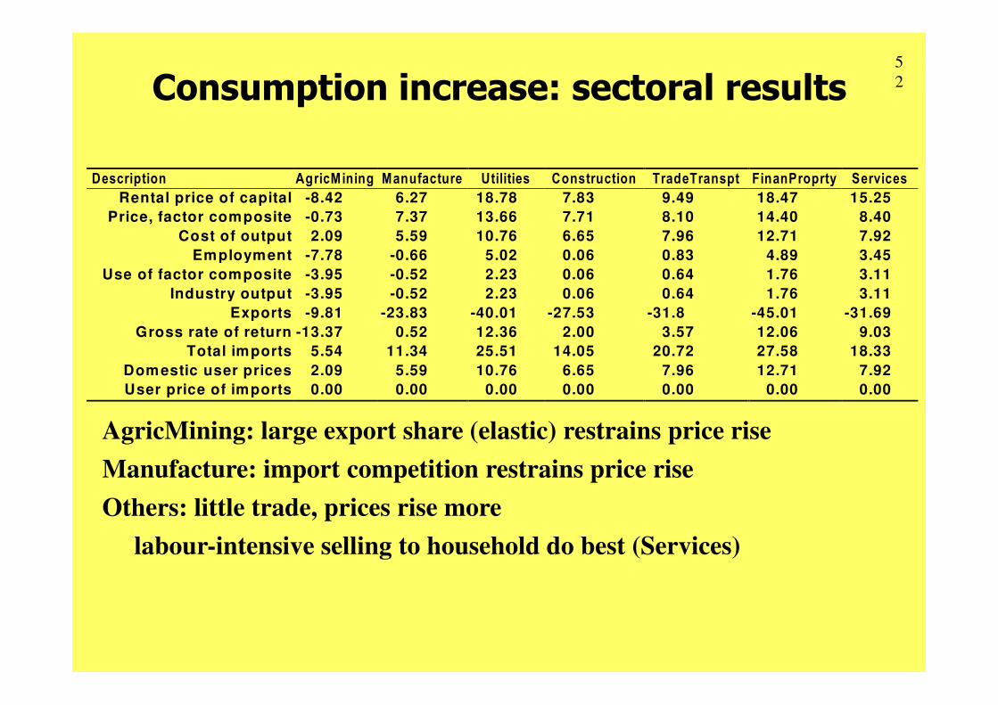
2Consumption increase: sectoral results
Description AgricMining Manufacture Utilities Construction TradeTranspt FinanProprty Services
Rental price of capital -8.42 6.27 18.78 7.83 9.49 18.47 15.25
Price, factor composite -0.73 7.37 13.66 7.71 8.10 14.40 8.40
Cost of output 2.09 5.59 10.76 6.65 7.96 12.71 7.92
Employment -7.78 -0.66 5.02 0.06 0.83 4.89 3.45
Use of factor composite -3.95 -0.52 2.23 0.06 0.64 1.76 3.11
Industry output -3.95 -0.52 2.23 0.06 0.64 1.76 3.11
Exports -9.81 -23.83 -40.01 -27.53 -31.8 -45.01 -31.69
Gross rate of return -13.37 0.52 12.36 2.00 3.57 12.06 9.03
Total imports 5.54 11.34 25.51 14.05 20.72 27.58 18.33Total imports 5.54 11.34 25.51 14.05 20.72 27.58 18.33
Domestic user prices 2.09 5.59 10.76 6.65 7.96 12.71 7.92
User price of imports 0.00 0.00 0.00 0.00 0.00 0.00 0.00
AgricMining: large export share (elastic) restrains price rise
Manufacture: import competition restrains price rise
Others: little trade, prices rise more
labour-intensive selling to household do best (Services)
5
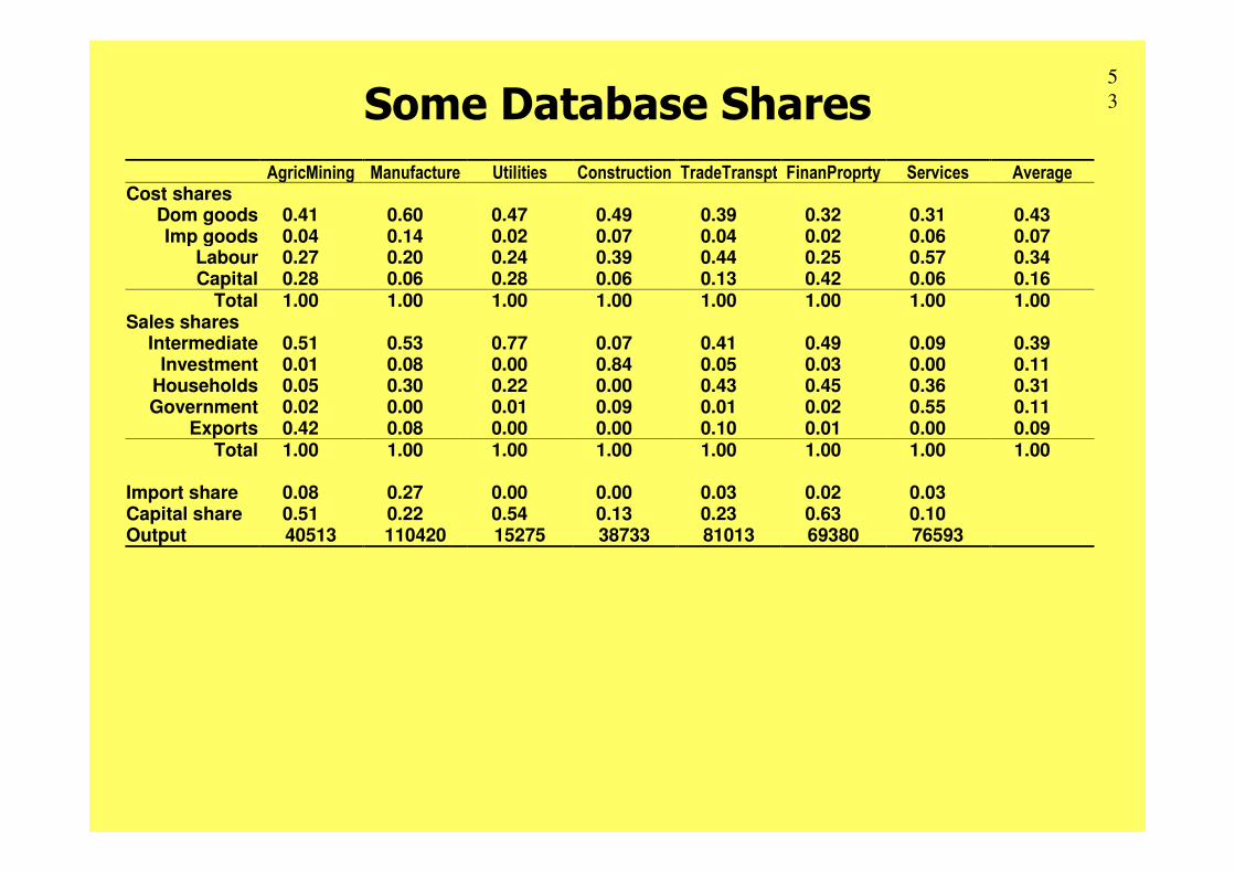
3Some Database Shares
AgricMining Manufacture Utilities Construction TradeTranspt FinanProprty Services AverageCost shares
Dom goods 0.41 0.60 0.47 0.49 0.39 0.32 0.31 0.43Imp goods 0.04 0.14 0.02 0.07 0.04 0.02 0.06 0.07
Labour 0.27 0.20 0.24 0.39 0.44 0.25 0.57 0.34Capital 0.28 0.06 0.28 0.06 0.13 0.42 0.06 0.16
Total 1.00 1.00 1.00 1.00 1.00 1.00 1.00 1.00Sales shares
Intermediate 0.51 0.53 0.77 0.07 0.41 0.49 0.09 0.39Investment 0.01 0.08 0.00 0.84 0.05 0.03 0.00 0.11
Households 0.05 0.30 0.22 0.00 0.43 0.45 0.36 0.31Government 0.02 0.00 0.01 0.09 0.01 0.02 0.55 0.11
Exports 0.42 0.08 0.00 0.00 0.10 0.01 0.00 0.09Exports 0.42 0.08 0.00 0.00 0.10 0.01 0.00 0.09Total 1.00 1.00 1.00 1.00 1.00 1.00 1.00 1.00
Import share 0.08 0.27 0.00 0.00 0.03 0.02 0.03Capital share 0.51 0.22 0.54 0.13 0.23 0.63 0.10Output 40513 110420 15275 38733 81013 69380 76593
5
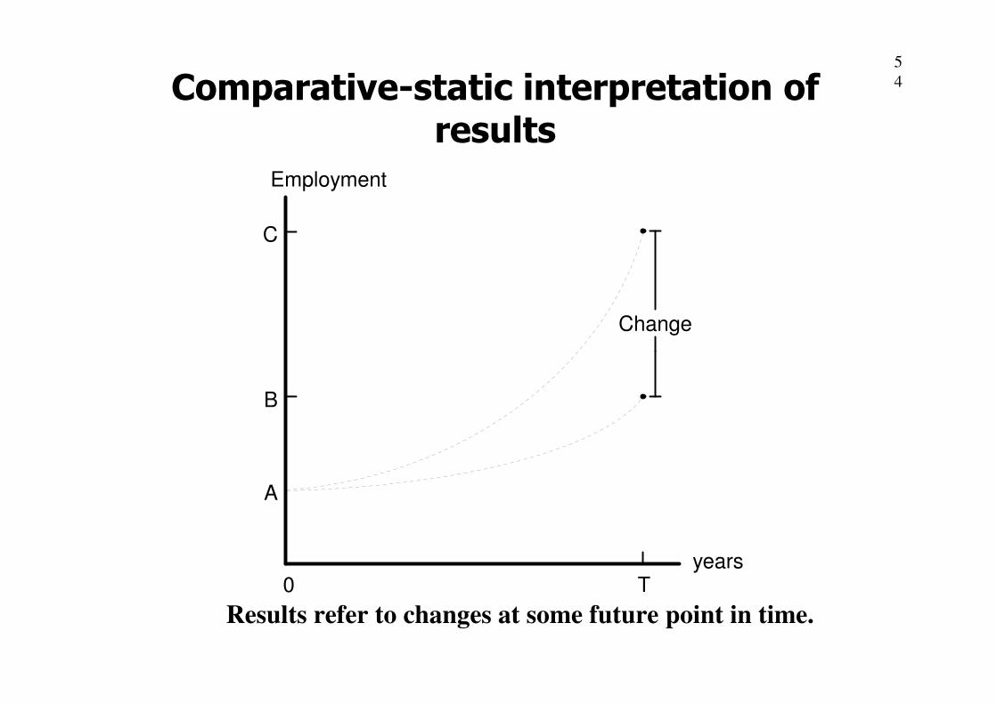
4Comparative-static interpretation of results
Employment
Change
C
Results refer to changes at some future point in time.
0 T
A
years
B

5
5
Length of run ,T
T is related to our choice of closure.
With shortrun closure we assume that:
•••• T is long enough for price changes to be transmitted throughout the economy, and for price-induced substitution to take place.
•••• T is not long enough for investment decisions to greatly affect •••• T is not long enough for investment decisions to greatly affect the useful size of sectoral capital stocks.[New buildings and equipment take time to produce and install.]
T might be 2 years. So results mean:
a 10% consumption increase might lead
to employment in 2 years time being 1.24% higher than it would be
(in 2 years time) if the consumption increase did not occur.
5
6
Features of more complex models
•••• more sectors.
•••• more primary factors: land, natural resources, types of labour.
•••• more final demanders: inventories, multiple households
•••• margin flows•••• margin flows
•••• commodity taxes specific to both commodity and user.
•••• multiproduction:one industry makes several commodities, or several industries make the same commodity.
• more technical change variables.
5
7
More features of more complex models
•••• consumption shares that depend on income as well as relative prices.
•••• more complicated production technology, with more types of substitution (eg, between capital and energy).
•••• more macro indices and other variables to help present results.present results.
•••• equations linking investment to profitability in each industry
•••• different investment technology for each industry.
•••• multiple regions (provinces, nations)
•••• multi-period models, which track through time
But still very similar to MINIMAL.


![IM PAN · 2017-10-17 · AUTOREFERAT 3 Osiągnięcie habilitacyjne: PROGRAM MODELI NIEMAL MINIMALNYCH I HIPOTEZA COOLIDGE’A-NAGATY [HAB1]Karol Palka, Cuspidal curves, minimal models](https://static.fdocuments.pl/doc/165x107/5f55af2fdbe37c478771ebbf/im-pan-2017-10-17-autoreferat-3-osignicie-habilitacyjne-program-modeli-niemal.jpg)